Spectral Maps for Learning Reduced Representations of Molecular Systems

Abstract

Presented at 34th IUPAP Conference on Computational Physics (CCP2023).
Investigating processes in complex molecular systems characterized by many variables is a crucial problem in computational physics. In theory, such systems can be reduced to a few meaningful degrees of freedom called collective variables (CVs). However, identifying CVs is a significant challenge, especially for the systems with long-lived metastable states, as information about the slow kinetics of rare transitions needs to be encoded in CVs. Here, we present our spectral map technique as a promising deep-learning method to learn CVs based on the slowest timescales. Spectral map maximizes the spectral gap between slow and fast eigenvalues of a Markov transition matrix constructed from simulation data. As an example, we show that our method can effectively capture a simplified representation of alanine dipeptide in solvent. Its ability to extract the slow CVs makes it a valuable tool for analyzing complex systems.

Reconstructing free-energy landscapes of systems as a function of slowly varying reaction coordinates, referred to as collective variables (CVs), is difficult, particularly due to the timescale limitations of molecular dynamics simulations [1]. Many machine learning techniques have been proposed to address this problem; see, for instance [2, 3, 4, 5, 6] and references therein. Nevertheless, accurately capturing the slow kinetics of rare transitions between metastable states still poses a challenge.

Among recent deep-learning techniques for identifying CVs presented during our talk [7, 8, 9, 10] is spectral map [11], which we consider here. As a simple demonstration of our method, we employ spectral map to extract a single CV describing the metastable states and underlying free-energy landscape of alanine dipeptide immersed in solvent.

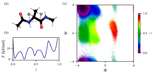
Figure 1: Example application of learning a slow CV using spectral map. (a) Alanine dipeptide in solvent with the $\Phi$ and $\Psi$ dihedral angles shown. As a high-dimensional representation, pairwise distances between heavy atoms are used ($n=45$), calculated from a dataset of three 250 ns trajectories. (b) Free-energy profile along the learned CV $z$ showing five distinct metastable states. (c) Alanine dipeptide conformations in the dihedral angle space are colored according to their CV value.

Consider a complex system with high-dimensional representation by $n$ configuration variables (or descriptors), $\mathbf{x}=(x_{1},\dots,x_{n})$. To make it easier to understand, we want to create a simplified representation by mapping the system into a low-dimensional manifold, $\mathbf{z}=(z_{1},\dots,z_{d})$, defined by a set of $d$ CVs, where $d\ll n$. As CVs are dependent on the configuration variables, we can express them as:

$$\mathbf{z}={\xi_{w}}(\mathbf{x})\equiv\big{\{}\xi_{k}(\mathbf{x}),w\big{\}}_{k=1}^{d},$$ (1)

where $\xi$ can be represented by a neural network with parameters denoted by $w$.

To extract the information about the intrinsic timescales of the system whose dynamics is represented in the CV space, we first estimate an anisotropic diffusion kernel [12]:

$$\kappa(\mathbf{z}_{k},\mathbf{z}_{l})=\frac{g(\mathbf{z}_{k},\mathbf{z}_{l})}{\sqrt{\rho(\mathbf{z}_{k})\rho(\mathbf{z}_{l})}},$$ (2)

where $g(\mathbf{z}_{k},\mathbf{z}_{l})=\exp(-\|\mathbf{z}_{k}-\mathbf{z}_{l}\|^{2}/\varepsilon)$ represents the Gaussian kernel, $\rho(\mathbf{z}_{k})=\sum_{l}g(\mathbf{z}_{k},\mathbf{z}_{l})$ denotes a kernel density estimate (up to normalization), $\|\mathbf{z}_{k}-\mathbf{z}_{l}\|$ stands for a pairwise distances between CV samples, and a scale constant is $\varepsilon$.

Next, we can build a Markov transition matrix by row-normalizing the diffusion kernel:

$$m_{kl}\sim M(\mathbf{z}_{k},\mathbf{z}_{l})=\frac{\kappa(\mathbf{z}_{k},\mathbf{z}_{l})}{\sum_{n}\kappa(\mathbf{z}_{k},\mathbf{z}_{n})},$$ (3)

which describes transition probabilities from $z_{k}$ to $z_{l}$. Then, we perform a spectral decomposition to estimate eigenvalues of the Markov transition matrix as $\lambda_{0}=1\geq\lambda_{1}\geq\lambda_{2}\geq\ldots$, which are used to calculate the spectral gap [11]:

$$\sigma=\lambda_{k{-1}}-\lambda_{k}$$ (4)

that measures the degree of the timescale separation between the slow and fast variables and $k$ denotes the number of metastable states in the CV space.

The main principle behind spectral map is that by using a parametrizable function $\mathbf{z}=\xi_{w}(\mathbf{x})$, we can adjust $w$ by maximizing the spectral gap, ensuring that the CV space is created by encoding slow degrees of freedom and treating fast variables as noise.

The algorithm for identifying slow CV using spectral map is composed of the following steps:

1. Dataset in a high-dimensional representation is collected from molecular dynamics simulations and used as input.

2. CVs $\mathbf{z}=\xi(\mathbf{x})$ expressed by a neural network are trained by maximizing the spectral gap and the degree of separation between slow and fast variables.

3. Trained CVs are used to build a free-energy landscape, $F(\mathbf{z})=-k_{\mathrm{B}}T\log P(\mathbf{z})$, where $P(\mathbf{z})$ is the probability distribution in the CV space, $T$ is the temperature, and $k_{\mathrm{B}}$ is the Boltzmann constant.

As a demonstration, we use spectral map to find slow CVs in a standard testing system for new methods, alanine dipeptide in solvent (Fig. 1a). As a dataset in a high-dimensional representation, we use three 250 ns molecular dynamics trajectories, carried out at 300 K, from the mdshare package. For more details on the dataset, we refer the reader to Ref [13]. Distances between the heavy atoms of alanine dipeptide ($n$ = 45) are employed as the configuration variables. No preprocessing is performed on the high-dimensional representation.

A 5-layer neural network of size [$n$, 50, 20, 10, $d$] is used. ReLU activation functions are applied between each hidden layer. The Adam optimizer is used with a learning rate of 0.0001. The dataset is split into data batches of 1000 samples, and the training is carried out through 100 epochs. Spectral map is trained to extract a slow CV for $k=5$ metastable states using a scale constant $\varepsilon$ of 0.001.

Our results are shown in Fig. 1. The free-energy profile along the learned slow CV shows five well-separated and long-lived metastable states with free-energy barriers higher than the thermal energy (Fig. 1b). This indicates that transitions between these states are rare and occur on longer timescales, i.e., the slow CV captures the most important slow processes of the system. Our results are in good agreement with Mardt et al [14].

During our talk, we reviewed the recent development of several unsupervised learning techniques for constructing CVs, including spectral map. Through a simple demonstration, we show that spectral map can offer valuable insights into the dynamics on longer timescales by capturing the slowest degrees of freedom and shows promise in analyzing molecular simulations of complex physical systems.

J.R. acknowledges funding from the Ministry of Science and Higher Education in Poland. J.R. and T.G. are supported by the National Science Center in Poland (Sonata 2021/43/D/ST4/00920, “Statistical Learning of Slow Collective Variables from Atomistic Simulations”).

References

- Valsson, Tiwary, and Parrinello [2016] O. Valsson, P. Tiwary, and M. Parrinello, “Enhancing Important Fluctuations: Rare Events and Metadynamics from a Conceptual Viewpoint,” Annu. Rev. Phys. Chem. 67, 159–184 (2016).
- Noé and Clementi [2017] F. Noé and C. Clementi, “Collective Variables for the Study of Long-Time Kinetics from Molecular Trajectories: Theory and Methods,” Curr. Opin. Struct. Biol. 43, 141–147 (2017).
- Wang, Ribeiro, and Tiwary [2020] Y. Wang, J. M. L. Ribeiro, and P. Tiwary, “Machine Learning Approaches for Analyzing and Enhancing Molecular Dynamics Simulations,” Curr. Opin. Struct. Biol. 61, 139–145 (2020).
- Chen [2021] M. Chen, “Collective Variable-Based Enhanced Sampling and Machine Learning,” Eur. Phys. J. B 94, 1–17 (2021).
- Chen and Chipot [2023] H. Chen and C. Chipot, “Chasing Collective Variables using Temporal Data-Driven Strategies,” QRB Discovery 4, e2 (2023).
- Rydzewski, Chen, and Valsson [2023] J. Rydzewski, M. Chen, and O. Valsson, “Manifold Learning in Atomistic Simulations: A Conceptual Review,” Mach. Learn.: Sci. Technol. 4, 031001 (2023).
- Rydzewski and Nowak [2016] J. Rydzewski and W. Nowak, “Machine Learning Based Dimensionality Reduction Facilitates Ligand Diffusion Paths Assessment: A Case of Cytochrome P450cam,” J. Chem. Theory Comput. 12, 2110–2120 (2016).
- Rydzewski and Valsson [2021] J. Rydzewski and O. Valsson, “Multiscale Reweighted Stochastic Embedding: Deep Learning of Collective Variables for Enhanced Sampling,” J. Phys. Chem. A 125, 6286–6302 (2021).
- Rydzewski et al. [2022] J. Rydzewski, M. Chen, T. K. Ghosh, and O. Valsson, “Reweighted Manifold Learning of Collective Variables from Enhanced Sampling Simulations,” J. Chem. Theory Comput. 18, 7179–7192 (2022).
- Rydzewski [2023a] J. Rydzewski, “Selecting High-Dimensional Representations of Physical Systems by Reweighted Diffusion Maps,” J. Phys. Chem. Lett. 14, 2778–2783 (2023a).
- Rydzewski [2023b] J. Rydzewski, “Spectral Map: Embedding Slow Kinetics in Collective Variables,” J. Phys. Chem. Lett. 14, 5216–5220 (2023b).
- Nadler et al. [2006] B. Nadler, S. Lafon, R. R. Coifman, and I. G. Kevrekidis, “Diffusion Maps, Spectral Clustering and Reaction Coordinates of Dynamical Systems,” Appl. Comput. Harmon. Anal. 21, 113–127 (2006).
- Wehmeyer and Noé [2018] C. Wehmeyer and F. Noé, “Time-Lagged Autoencoders: Deep Learning of Slow Collective Variables for Molecular Kinetics,” J. Chem. Phys. 148, 241703 (2018).
- Mardt et al. [2018] A. Mardt, L. Pasquali, H. Wu, and F. Noé, “VAMPnets for Deep Learning of Molecular Kinetics,” Nat. Commun. 9, 5 (2018).