Time-optimal Design and Control of Electric Race Cars Equipped with Multi-speed Transmissions

Abstract

This paper presents a framework to jointly optimize the design and control of an electric race car equipped with a mgt, specifically accounting for discrete gearshift dynamics. We formulate the problem as a miocp, and deal with its complexity by combining convex optimization and pmp in a computationally efficient iterative algorithm satisfying necessary conditions for optimality upon convergence. Finally, we leverage our framework to compute the achievable lap time of a race car equipped with a fgt, a cvt and an mgt with 2 to 4 speeds, revealing that an mgt can strike the best trade-off in terms of electric motor control, and transmission weight and efficiency, ultimately yielding the overall best lap time.

I Introduction

The electrification of automotive powertrains has sparked significant attention over the last years. Conventional passenger vehicles are being replaced by hybrid and fully electric vehicles [1], while existing racing classes are also hybridized, and new fully electric racing classes are emerging. In motorsport, every millisecond counts, so all involved technologies are pushed to their limits. For electric racing, the available battery energy is a significant limitation, which means that optimal energy management and em efficiency can make the difference to win a race. To achieve maximum performance while keeping the em within its most efficient operating range, various transmission types can be used, which yield control over the em operating range, at the cost of the transmission’s own efficiency and weight. At one end of the spectrum, the fgt is light and efficient, while providing little control over the operating range of the em. At the other end, the cvt provides continuous control over the em operation, but at the cost of increased weight and a lower efficiency. Between these extremes, a mgt could balance the efficiency of an fgt with the operating range control of a cvt. To select the optimal transmission for any given application, a joint optimization of transmission design and powertrain control is required. However, the gearshifts of an mgt introduce discrete dynamics, which turns the optimization of an mgt-equipped race car into a miocp. miocps are generally $\mathcal{NP}$-hard, and can be very difficult to solve [2]. Against this backdrop, this paper presents a computationally efficient algorithm for the optimization of the design and control of an mgt-equipped electric race car.

Figure 1: Schematic layout of the electric race car powertrain under consideration, consisting of a battery (BAT), an inverter (INV), an electric motor (EM), a transmission (GB) and the wheels (W). The gear-ratio $\gamma$ is a control input that must be chosen from a finite (FGT and MGT) or continuous (CVT) set, which is in turn subject to design. The arrows indicate power flows between components.

Related literature: The mixed-integer time-optimal design and control problem studied in this paper pertains to two main research streams, namely, energy management and time-optimal control of (hybrid) electric vehicles.

For energy management, mainly non-causal optimization is applied on drive cycles with known velocity and torque requirements. Joint optimization of the gearshift strategy and gear ratio design has been carried out using dynamic programming [3], combined dynamic programming and convex optimization [4] and mixed-integer nonlinear optimization [5]. For the design and control of an fgt- and cvt-equipped vehicle, convex optimization is employed by [6, 4]. However, since these methods use known drive cycles, none of them can be directly applied to time-optimal control problems, where the velocity trajectory is unknown.

For the time-optimal control of race cars, [7] proposes a distance-based convex optimization framework, which is extended to consider the design and control of an fgt and cvt in [8]. In [9], the mgt gearshift is optimized by using iterative dynamic programming with pmp and convex optimization, while [10] uses outer convexification and nonlinear programming to optimize the gearshift. However, both methods lack optimality guarantees and solely focus on control strategies.

In conclusion, to the best of the authors’ knowledge, there are no frameworks for time-optimal control of race cars considering both gearshifts and gear ratio design.

Statement of Contributions: This paper provides a computationally efficient framework to optimize the design and control of the electric race car powertrain shown in Fig. 1. To this end, we introduce an efficient iterative algorithm to optimize the mgt-equipped race car, combining convex optimization with pmp to efficiently account for the discrete gearshift dynamics. Finally, we leverage our algorithm to compare the performance of a race car equipped with an fgt, a cvt and an mgt with 2 to 4 speeds on the Zandvoort race track.

II mgt Optimization Methodology

In this section, we define the minimum-lap-time design and control problem for the powertrain shown in Fig. 1, together with algorithms to solve the optimization problems.

II-A Optimization Problem Definition

We base our optimization framework on the convex framework developed in [8] for the time-optimal design and control of an fgt- and a cvt-equipped race car, while we include an mgt model, and the more accurate vehicle dynamics and inverter models from [11]. This provides us with a minimum-lap-time design and control problem in the space-domain, which grants us a finite problem horizon $S$, and allows us to optimize over the position on track $s$. For the sake of brevity, we do not show our component models here.

Before defining our optimization problem, we divide our optimization variables as follows: First, we consider the design variables: $p=\gamma_{1}$ for the fgt, $p=\{\gamma_{1},\dots,\gamma_{n_{\mathrm{gear}}}\}$ for the mgt and $p=\gamma_{\mathrm{max}}$ for the cvt. Here, $\gamma_{i}$ is the ratio of gear $i$, $n_{\mathrm{gear}}$ is the total number of mgt gears, and $\gamma_{\mathrm{max}}$ is the maximum ratio for the cvt. For notational convenience, we model the design variables as state variables with zero dynamics,

$$\frac{\mathrm{d}\gamma_{i}(s)}{\mathrm{d}s}=0,$$

which leaves only the initial conditions as free optimization variables. With this, we consider the state variables as $x=\{E_{\mathrm{bat}},E_{\mathrm{kin}},p\}$, where $E_{\mathrm{bat}}$ and $E_{\mathrm{kin}}$ are the battery energy and kinetic energy of the vehicle, respectively. As control inputs we consider $u=\{F_{\mathrm{m}},F_{\mathrm{brk,F}},F_{\mathrm{brk,R}}\}$, where $F_{\mathrm{m}}$ is the mechanical motor force, assuming a rear-wheel driven vehicle, and $F_{\mathrm{brk,F}}$ and $F_{\mathrm{brk,R}}$ are the brake forces at the front and rear axle, respectively. For the cvt we further consider the gear ratio at a given position on track $\gamma(s)$ as an input variable, whilst for the mgt we consider the additional input $b(s)\in\{0,1\}^{n_{\mathrm{gear}}}$, which is a binary variable stating the active gear at a given position on track. With this, we formulate our problem to minimize the lap time $T$ as follows:

Problem 1 (Minimum-lap-time problem).

The time-optimal design and control strategies are the solution of

$$\!\min_{x,u}T,$$

$$\begin{aligned} \textnormal{s.t. }&\textnormal{State dynamics and limits},&&&&\\ &\textnormal{Vehicle dynamics and limits,}&&\\ &\textnormal{Component models.}&&\end{aligned}$$

Since all models and variables for the fgt and cvt optimization problems are continuous and convex, Problem 1 can be solved for the globally optimal solution in polynomial time [12] using commercially available solvers. Conversely, due to the binary gearshift variable $b$, the mgt optimization problem is a miocp, which is computationally demanding, and often even intractable, hence calling for an alternative solution scheme, which we outline in Section II-B below.

II-B Iterative algorithm

In this section, we describe the iterative algorithm, shown in Fig. 2, used to solve the optimal design and control problem of an mgt-equipped race car. We subdivide the miocp into a cp, which optimizes the continuous design and control variables for a given gearshift trajectory, and a gp, which optimizes the gearshifts for a given state and costate trajectory. We iterate between these problems until the results converge, using dampened costate trajectories to ensure convergence. To distinguish between iterations of our algorithm, we introduce the $(\cdot)^{k}$ notation to describe the current iteration $k\in\mathbb{N}$. To improve readability, we group our continuous inputs as $c=\{F_{\mathrm{m}},F_{\mathrm{brk,F}},F_{\mathrm{brk,R}}\}$. Finally, since the continuous inputs are optimized by both the cp and gp, we distinguish between the results of the respective problems using a $(\cdot)_{\mathrm{C}}$ and $(\cdot)_{\mathrm{G}}$ notation.

Figure 2: Iterative algorithm for the optimization of an electric race car equipped with an mgt. Given an initial gearshift trajectory $b^{0}$, the continuous variables are optimized in the COP. The resulting state and costate trajectories $(x,\lambda)$ are then used to re-optimize the gearshift trajectory in the GOP. These steps are iterated until the results converge.

II-C Continuous Optimization Problem Definition

By providing a pre-determined trajectory $b^{k-1}(s)$, we can optimize our continuous variables using the convex cp.

Problem 2 (Continuous Optimization Problem).

We define the cp for mgt optimization as

$$(x^{k},c^{k}_{\mathrm{C}})=\arg\min_{x,c}T,$$

$$\begin{aligned} \textnormal{s.t.:}~{}&\textnormal{State dynamics and limits,}&&&&\\ &\textnormal{Vehicle dynamics and limits,}&&\\ &\textnormal{Component models,}&&\\ &b(s)\coloneqq b^{k-1}(s)&&\forall s\in[0,S].&&\end{aligned}$$

This fully convex cp can be solved in polynomial time, similar to Problem 1 for the fgt and cvt.

II-D Gearshift Optimization Problem Definition

We optimize the binary gearshift trajectory by applying pmp, which allows us to efficiently solve the problem for each position on track independently. According to pmp [13], the optimal solution satisfies

$$(u^{\star})=\arg\underset{u}{\min}~{}\mathcal{H}(x^{\star},\lambda,u),$$

where $(\cdot)^{\star}$ denotes an optimal trajectory, $\mathcal{H}$ is the Hamiltonian, and $\lambda$ represents the costates. If we provide a pre-determined state and costate trajectory $(x,\lambda)$, the Hamiltonian minimization problem can be solved at every position on track independently, thereby significantly reducing the computational complexity. By minimizing the Hamiltonian for each gear option separately with convex optimization, the optimal trajectory can be determined by selecting the Hamiltonian with the minimum value at each position, which can be done in polynomial time. By providing a pre-determined state and costate trajectory $(x^{k}(s),\lambda^{k}(s))$, and by omitting the state dynamics and limits, we formulate the gp as follows:

Problem 3 (Gearshift Optimization Problem).

We define the gp for mgt optimization as

$$(b^{k},c^{k}_{\mathrm{G}})=\arg\min_{b,c}\mathcal{H}(s),$$

$$\begin{aligned} \textnormal{s.t.:}~{}&\textnormal{Vehicle dynamics and limits,}&&\\ &\textnormal{Component models,}&&\\ &\begin{cases}x(s)\coloneqq x^{k}(s)\\ \lambda(s)\coloneqq\lambda^{k}(s)\\ \end{cases}&&\forall s\in[0,S].&&\end{aligned}$$

II-E Discussion

Since the cp and gp both minimize lap time, iterating between the two will yield a situation where neither problem can independently yield an improved lap time that is feasible for the original problem. Since we dampen our costate trajectories between iterations, the gearshift trajectory converges at this point, which results in convergence of all other trajectories. In our extended work, we provide formal proofs showing that at convergence our solutions satisfy necessary conditions for optimality. The combination of these findings—even if not sufficient—with the quality and consistency of the numerical results provided in Section III below is promising.

III Results and Validation

This section presents the results obtained by applying our framework to various transmission types. We first evaluate the performance of each transmission over a racing lap, and then validate the performance of our iterative algorithm.

III-A Numerical Results

In this section, we apply our framework to one lap around the 4.2 km long Zandvoort race track, using the InMotion LMP3 race car [14] as a demonstrator. We solve Problem 1 for the fgt- and cvt-equipped cars, and apply the iterative algorithm for the cars with a 2gt, a 3gt and a 4gt. To realistically compare performance, we include the transmission weight in our simulation. With respect to the fgt-equipped car, each added gear in an mgt increases the total vehicle weight by 0.37 %, while the cvt increases the vehicle weight by 2.6 %. We parse the problems with YALMIP [15], using a forward Euler discretization and a step of $\Delta s=4$ m, and solve with MOSEK [16] on a laptop with a 2.6 GHz processor and 16 GB RAM. Problem 1 takes on average 1.2 s to solve for the fgt and 1.4 s for the cvt, while the iterative algorithm converges in about 63 s on average. Fig. 3 shows that the algorithm gets close to the final converged lap time within a few iterations, while we observe no conclusive correlation between the number of gears and the amount of iterations required for convergence.

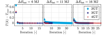
Figure 3: Convergence of the iterative algorithm, showing the difference between the lap time at each iteration and the final converged lap time $(T_{\mathrm{conv}})$. Results are shown for multiple battery energy consumption limits.

Fig. 4 and Fig. 5 present the results for a case where the vehicle is significantly energy-limited. As can be observed, the cvt-equipped car performs considerably worse than the others, due to its lower internal efficiency and higher weight. The 2gt-car, instead, outperforms the fgt-car due to the increased em efficiency, which allows it to accelerate faster and regeneratively brake both later and more aggressively. The 3gt-car contains an added gear with a very low ratio, which allows for a high em efficiency at high speed but low power sections. In combination with a higher first gear ratio, this allows the 3gt-car to accelerate faster out of corners compared to the 2gt-car, yielding even faster lap times. However, the 4gt-car cannot provide enough additional performance with its added gear to compensate for its higher weight, rendering it marginally slower than the 2gt-car. In conclusion, using a 3gt yields the best trade-off between control freedom and weight for the case presented here.

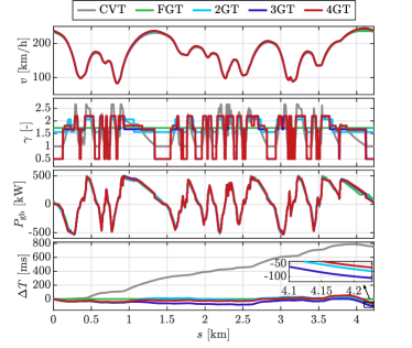
Figure 4: Velocity, gear ratio, and transmission output power trajectories for each car, in battery-limited operation. To compare, we also show the relative lap time of each car with respect to the fgt-equipped car.

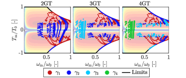
Figure 5: Operating points of the em for each mgt-equipped car.

III-B Validation

In order to validate the efficacy of the iterative algorithm, we solve the miocp directly using the MOSEK mixed-integer second-order cone programming solver, which employs a branch-and-bound algorithm to solve the problem with global optimality guarantees. Due to the complex nature of our problem, the mixed-integer solver can only solve for a discretization of $N_{\mathrm{steps}}=22$ steps in less than $10$ hours, requiring exponentially more time for each added step. Since the original problem contains $N_{\mathrm{steps}}=1058$ steps, this means that the mixed-integer solver is only able to solve a section with a length of about 2 % of the lap within $10$ hours. Therefore, we validate the iterative algorithm by using a coarser discretization, and by optimizing only a small section of the track, containing a braking zone, a corner, and an acceleration zone. To exemplify the computational complexity of our problem, we present the computation times for the mixed-integer solver and iterative algorithm for a varying number of discretization steps in Table I. As can be observed, the mixed-integer algorithm soon becomes intractable, while the iterative algorithm obtains virtually the same section times in much less computation time. Only for one simulation is the section time obtained by the iterative algorithm 0.3 milliseconds slower, probably due to a poor initial guess. Overall, this validation shows that the iterative algorithm can provide very promising solutions.

TABLE I: Computation time comparison between a mixed-integer solver and the iterative algorithm on a short track section.

	Mixed-integer		Iterative
	Solving time	Section time	Solving time	Section time	Section time difference
${N_{\mathrm{steps}}}$
12	43 s	3.5946 s	2 s	3.5946 s	0.0 ms
14	120 s	3.4959 s	2 s	3.4959 s	0.0 ms
16	575 s	3.4256 s	2 s	3.4259 s	0.3 ms
18	1940 s	3.3403 s	2 s	3.3403 s	0.0 ms
20	8153 s	3.4759 s	2 s	3.4759 s	0.0 ms
22	34915 s	3.4302 s	2 s	3.4302 s	0.0 ms

IV Conclusion

In this paper, we presented a framework to optimize the design and control of an electric race car, considering a cvt, a fgt and a mgt. To this end, we developed an iterative algorithm to efficiently handle the mixed-integer mgt gearshifts, combining convex optimization and pmp. We demonstrated that our algorithm satisfies necessary conditions for optimality upon convergence, and corroborated this with numerical results showing convergence to promising solutions in terms of optimality. Finally, we studied the performance of the various transmissions on the Zandvoort race track, where we observed that an mgt can balance the individual advantages of both an fgt and a cvt, by delivering significant control over the em operating range at a low cost in terms of transmission weight and efficiency loss. Interestingly, we also noted that adding one gear too many can be detrimental to the lap time, highlighting the importance of carefully choosing the right transmission technology and design for specific car and track requirements. In a future extended work we will provide detailed models, formal proofs, and design studies over a range of battery energy levels and em scales.

References

- [1] IEA, “Global EV outlook 2021,” International Energy Agency, Tech. Rep., 2021.
- [2] S. Sager, “Numerical methods for mixed-integer optimal control problems,” Ph.D. dissertation, Universität Heidelberg, 2005.
- [3] B. Gao, Q. Liang, Y. Xiang, L. Guo, and H. Chen, “Gear ratio optimization and shift control of 2-speed i-amt in electric vehicle,” Mechanical Systems and Signal Processing, vol. 50-51, pp. 615–631, 2015.
- [4] J. van den Hurk and M. Salazar, “Energy-optimal design and control of electric vehicles’ transmissions,” in IEEE Vehicle Power and Propulsion Conference, 2021, in press. Extended version available at https://arxiv.org/abs/2105.05119.
- [5] H. Yu, F. Zhang, J. Xi, and D. Cao, “Mixed-integer optimal design and energy management of hybrid electric vehicles with automated manual transmissions,” IEEE Transactions on Vehicular Technology, vol. 69, no. 11, pp. 12 705–12 715, 2020.
- [6] F. J. R. Verbruggen, M. Salazar, M. Pavone, and T. Hofman, “Joint design and control of electric vehicle propulsion systems,” in European Control Conference, 2020.
- [7] S. Ebbesen, M. Salazar, P. Elbert, C. Bussi, and C. H. Onder, “Time-optimal control strategies for a hybrid electric race car,” IEEE Transactions on Control Systems Technology, vol. 26, no. 1, pp. 233–247, 2018.
- [8] O. Borsboom, C. A. Fahdzyana, T. Hofman, and M. Salazar, “A convex optimization framework for minimum lap time design and control of electric race cars,” IEEE Transactions on Vehicular Technology, vol. 70, no. 9, pp. 8478–8489, 2021.
- [9] P. Duhr, G. Christodoulou, C. Balerna, M. Salazar, A. Cerofolini, and C. H. Onder, “Time-optimal gearshift and energy management strategies for a hybrid electric race car,” Applied Energy, vol. 282, no. 115980, 2020.
- [10] C. Balerna, M.-P. Neumann, N. Robuschi, P. Duhr, A. Cerofolini, V. Ravaglioli, and C. Onder, “Time-optimal low-level control and gearshift strategies for the formula 1 hybrid electric powertrain,” Energies, vol. 14, no. 1, 2021.
- [11] J. van Kampen, T. Herrmann, T. Hofman, and M. Salazar, “Optimal endurance race strategies for a fully electric race car under thermal constraints,” IEEE Transactions on Control Systems Technology, 2023, under Review.
- [12] S. Boyd and L. Vandenberghe, Convex optimization. Cambridge Univ. Press, 2004.
- [13] D. Bertsekas, Dynamic programming and optimal control, 4th ed. Athena Scientific, 1995.
- [14] (2023) InMotion fully electric LMP3 car. InMotion. Available at https://www.inmotion.tue.nl/en/about-us/cars/revolution.
- [15] J. Löfberg, “YALMIP : A toolbox for modeling and optimization in MATLAB,” in IEEE Int. Symp. on Computer Aided Control Systems Design, 2004.
- [16] Mosek APS. The MOSEK optimization software. Available at http://www.mosek.com.