The IFU data returned by MUSE are 3D cubes, with 2 spatial dimensions, and one spectral dimension, meaning each pixel of the image has an associated spectrum. A number of data products have been made available from the MAD survey, including 2D maps of dust-corrected emission line fluxes for all strong lines within the observed wavelength range. However, for our analysis we require flux maps for additional weak, auroral emission lines, as well as associated line flux uncertainties, which are not readily available. We therefore produce our own emission line maps from the reduced MUSE data cubes, which we download from the ESO archive science portal.

In order to measure accurate emission line fluxes, we first need to separate the stellar and gas emission components in order to correct for Balmer absorption from old stellar populations. A failure to correct for such stellar absorption features can result in the Balmer line fluxes being underestimated, increasingly so for bluer Balmer lines, thus affecting the measured Balmer decrement which we need to produce galaxy dust reddening maps. We use the starlight software package to separate the stellar and gas emission components (CidFernandes2005; CidFernandes2009), following a similar procedure as described in Kruhler2017. In summary, we use starlight to fit a linear superposition of template spectra to each $2\times 2$ binned MUSE spectrum, using the stellar population models from Bruzual2003. At the typical redshift of our galaxy sample ($z\sim 0.005$), the $2\times 2$ spatial binning corresponds to a physical size of $\sim$40 pc, reaching up to 100 pc for the most distant galaxy in our sample (NGC3393). We then linearly scale the best-fit stellar template to the intensity of each of the four spaxels in our bin, and subtract this weighted stellar component from the original data to produce a gas-phase only cube.

We removed NGC3521 from the sample, as it has very weak emission lines, and low S/N of the  and auroral lines. NGC4593 was also removed, due to the large contribution of and active galactic nucleus in the centre, leaving us with a final sample of 36 galaxies.

0.1 region identification with HIIdentify

90

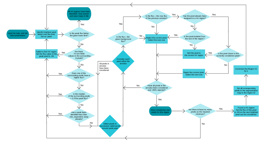
Figure 1: Flowchart illustrating the steps taken by to identify pixels as being peaks of regions, removing any spaxels determined to be noise within the image, and to then assign pixels to the regions, returning segmentation maps as shown in Fig. 2.

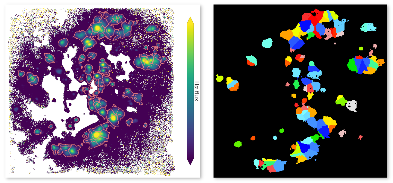
Figure 2: Left:  flux map of NGC1483, with outlines of the regions identified with shown in red. Right: Segmentation map, where the pixels within each region are set to the region ID number, shown here by different colours.

To identify regions within each galaxy, we use maps of the  flux, masking out all spaxels with equivalent width of $<$ 6 Å, which are associated with Diffuse Ionised Gas (DIGs) rather than star forming (SF) regions. DIGs have different physical properties to regions, with lower gas densities, and lower ionisation parameters. The ionising source for DIGs has not been conclusively determined, meaning the metallicity diagnostics which have been calibrated against observations and models of the gas within regions are not expected to remain valid when used on DIGs (e.g. Sanders2017; Zhang2017; Lacerda2018a). Our choice of a threshold of 6 Å is a compromise between the recommendations of Sanchez2015, Belfiore2016 and Lacerda2018a (see also Belfiore2017). However our results are not very sensitive to the choice of the  threshold that we use, and increasing this cut to 14 Å, as suggested by Lacerda2018a to identify purely star-forming regions, was found to have little effect on the regions identified using the process described below.

We developed a python tool, which we have named , to automatically identify regions within a galaxy based on the emission, following a similar methodology to codes such as HIIphot (Thilker2000) and pyHIIexplorer (Espinosa-Ponce2020). To identify regions, iterates through the pixels from the brightest to the dimmest, terminating at a user-defined lower limit on the flux. Each of these pixels are considered as a possible peak of a region, using several criteria to exclude noise within the image, as shown in Fig. 1. For example the peak is rejected if $>50\%$ of the surrounding pixels have non-finite flux values, or if the median flux of the surrounding pixels is $<30\%$ of that of the peak. Other criteria must also be met for the pixel to be confirmed as the peak of a region – all of the immediately surrounding pixels must have lower fluxes than the currently considered peak, and a minimum required separation between regions can be specified. For this analysis, we used a minimum separation of 50 pc.

Once a pixel is successfully identified as the peak of a region, surrounding pixels are considered in circular annuli, and are added to the region if the flux is greater than the user-defined background flux, and the pixel has not already been added to another region. If a pixel is selected to belong to multiple regions, it is assigned to the region with the closest peak. The radius of the regions is not constrained, and instead the growth of the region stops when $>80\%$ of the pixels in the annulus have been rejected.

Finally, a minimum required number of pixels can be specified, which sets a lower limit on the number of pixels any identified region must have. Once all possible regions have been identified according to the criteria described above, our code creates a number of maps, including a segmentation map, which depicts which region each pixel belongs to, if any.  is publicly available for download, with information on how to install and use it provided in the online documentation. An example MUSE  map from the MAD sample can be seen in Fig 2, with the outlines of identified regions overlaid. The associated segmentation map is also shown, indicating the spaxels belonging to each of the identified regions. As there are no constraints on the shape or size of the identified regions, it can be seen that identifies all regions with peak flux above a user-defined level, and encapsulates all of the surrounding region out to a given background level, rather than making assumptions about the geometry of the regions.

The results from applying to our sample are shown in Table 1, and the returned segmentation maps have been made publicly available. Input parameters were set so as to ensure that the entire region was encapsulated, with any low S/N spaxels removed at a later stage. The background flux was determined using spaxels with S/N ¿ 3, and ¡ 14 Å, selecting the 75th percentile of the flux to represent the background level at which to set the edge of the regions. Using the above input parameters, a total of 4408 regions were identified in our sample of 36 galaxies, and they generally had a radius of a few hundred parsecs, which is consistent with observed sizes of regions.

Following the release of the MUSE-PHANGS (Physics at High Angular resolution in Nearby GalaxieS; Emsellem2022) catalogue in Groves2023, which included segmentation maps from the code, in Appendix LABEL:app:hiidentifyhiiphot we compare the results from the two codes, finding very good agreement in the resulting metallicity measurements.

Table 1: The stellar mass ($M_{*}$), star formation rate (SFR), and number of regions identified by in the 36 MAD galaxies in our sample. We also list the number of regions in each galaxy that have  S/N $>$ 5 and nebular S/N ¿ 3, and thus were included in our final sample.

Galaxy	log$(M_{*})$	SFR	Num.	S/N sel.
	[M⊙]	[M⊙/yr]	regions	regions
NGC4030	11.18	11.08	418	43	(10%)
NGC3256	11.14	3.10	132	39	(30%)
NGC4603	11.10	0.65	248	0	(0%)
NGC3393	11.09	7.06	17	0	(0%)
NGC1097	11.07	4.66	58	8	(14%)
NGC289	11.00	3.58	133	14	(11%)
IC2560	10.89	3.76	167	30	(18%)
NGC5643	10.84	1.46	95	10	(11%)
NGC3081	10.83	1.47	48	0	(0%)
NGC4941	10.80	3.01	18	2	(11%)
NGC5806	10.70	3.61	141	16	(11%)
NGC3783	10.61	6.93	102	35	(34%)
NGC5334	10.55	2.45	122	12	(10%)
NGC7162	10.42	1.73	62	0	(0%)
NGC1084	10.40	3.69	201	38	(19%)
NGC1309	10.37	2.41	257	48	(19%)
NGC5584	10.34	1.29	78	13	(17%)
NGC4900	10.24	1.00	352	43	(12%)
NGC7496	10.19	1.80	140	16	(11%)
NGC7552	10.19	0.59	139	20	(14%)
NGC1512	10.18	1.67	30	1	(3%)
NGC7421	10.09	2.03	70	9	(13%)
ESO498-G5	10.02	0.56	16	0	(0%)
NGC1042	9.83	2.41	44	5	(11%)
IC5273	9.82	0.83	94	17	(18%)
NGC1483	9.81	0.43	97	34	(35%)
NGC2835	9.80	0.38	100	14	(14%)
PGC3853	9.78	0.35	47	6	(13%)
NGC337	9.77	0.57	119	1	(1%)
NGC4592	9.68	0.31	325	79	(24%)
NGC4790	9.60	0.39	208	38	(18%)
NGC3513	9.37	0.21	108	17	(16%)
NGC2104	9.21	0.24	90	11	(12%)
NGC4980	9.00	0.18	89	34	(38%)
NGC4517A	8.50	0.10	19	10	(53%)
ESO499-G37	8.47	0.14	24	8	(33%)

0.2 Spectral line fits

To measure the line fluxes within each spaxel, we fitted the emission lines of interest with Gaussian functions using the specutils package in python.

The lines were grouped into chunks with nearby lines (e.g. the  and $\lambda\lambda$6549,84 lines) when fitting, so that the positions could be tied to that of the brightest line to help constrain the fits, and in the case of doublets, the widths could be tied and the ratio of the amplitudes fixed to known theoretical ratios when fitting. The continuum extending $\sim$ 50Å either side of the lines was included, allowing the continuum level to be fitted when determining line fluxes. The $\lambda\lambda$6302,65 sky lines were masked out before fitting the lines. The cube slice was dust-corrected using dust reddening maps that were produced from the measured -to- Balmer decrement, and assuming a Cardelli1989 attenuation law. We assumed an intrinsic Balmer decrement of 2.87 (Osterbrock2006), suitable for star forming galaxies with electron density $\sim$100cm^-3 and temperature $\sim$10,000K.

For the $\lambda$9531 line, required for our -based measurements, we use the known theoretical flux ratio between $\lambda$9070 and $\lambda$9531 of 2.47 (Luridiana2015), along with our measured flux for the $\lambda$9070 line.