Correlation, crossover and broken scaling in the Abelian Manna Model

Abstract

The role of correlations in self-organised critical (SOC) phenomena is investigated by studying the Abelian Manna Model (AMM) in two dimensions. Local correlations of the debris left behind after avalanches are destroyed by re-arranging particles on the lattice between avalanches, without changing the one-point particle density. It is found that the spatial correlations are not relevant to small avalanches, while changing the scaling of the large (system-wide) ones, yielding a crossover in the model’s scaling behaviour. This crossover breaks the simple scaling observed in normal SOC.

I INTRODUCTION

Spatial correlations are at the core of self-organised critical (SOC) phenomena, because part of the narrative of SOC is the spreading of long-range spatial correlations as systems evolve towards the critical point Watkins et al. (2016). Correlations between (but also within) avalanches are thought to be mediated by “substrate particles” Dickman et al. (1998), i.e. , the immobile particles left behind by avalanches. These are replenished by the repeated external driving and form the fuel and backdrop of the next avalanche. Despite the great conceptual importance to SOC, spatial correlations are rarely studied directly, as they are notoriously noisy and difficult to analyse Pruessner (2012). In the Manna Model Manna (1991); Dhar (1999), Hexner and Levine Hexner and Levine (2015) identified hyperuniformity in the substrate particle density and Basu et al. Basu et al. (2012) observed “natural long-range correlations in the background”. Using the fact that natural critical states in the Oslo rice pile model are hyperuniform, Grassberger et al. Grassberger et al. (2016) were able to perform vastly improved simulations. Recently, one of us Willis and Pruessner (2018) found the algebraic auto-correlations of immobile substrate particles in the Manna Model to display hyperuniformity with comparatively small amplitude when measured directly. As the density of immobile particles is bounded, the amplitude of their auto-correlations cannot increase with system size. If coarse graining was to be applied, any such correlations can therefore be made arbitrarily small at any non-vanishing distance, in contrast to the invariance under rescaling normally observed in critical phenomena and confirmed for the activity in the Manna Model Willis and Pruessner (2018).

Similarly, the density of immobile particles as a function of position on the lattice (introduced as the “density profile” $\rho(x,y)$ below) rises quickly away from the boundaries, remains (almost) constant in the bulk and then drops sharply again at the other boundary, Fig. 1 in Willis and Pruessner (2018).

The aim of the present work is to determine whether the correlations of substrate particles have a bearing on the critical state in the sense of being a prerequisite of the critical behaviour in the Manna Model, rather than being a result of it. Are these correlations weak but important, or weak and irrelevant?

One may attempt to address this question by redistributing particles uniformly in the stationary state. In the Manna Model this was investigated by Stapleton (Chapter 5 in Stapleton (2007)) in one dimension, resulting in scaling compatible with the Manna universality class. One of us repeated some of these numerical experiments on much bigger lattices (Pruessner, 2012, p. 172, 173) and found deviating exponents, albeit non-trivial ones. However, by redistributing, not only the correlations are destroyed, but also the density profile is evened out. Field-theoretically, the density profile is expected to be more relevant than the two-point correlation function Lee and Cardy (1995) not least as its shape has a direct impact on particle transport towards boundaries Paczuski and Bassler (2000) and thus on the avalanche size at the stationary state. We will therefore test the relevance of the correlations by removing or diluting any auto-correlations that may have developed over the course of an avalanche without, however, destroying the density profile. We will then probe whether the critical behaviour is effected.

At this stage, we deliberately allow for ambiguity in the notion of “bearing on the critical behaviour” — a possible outcome may be that after tempering with the substrate particle distribution the Manna Model remains critical, yet displays scaling behaviour different from that of the Manna universality class. Another outcome may be loss of all (non-trivial) critical behaviour whatsoever.

In the following, we will first introduce the Manna Model and the relevant observables in detail in Sec. II.1, then show different setups used to destroy the correlations in the substrate in Sec. II.2. The results are presented in Sec. III and Appendix A. In Sec. IV, we will discuss the different exponents we find and the role of correlations. Sec. V contains a summary of our results, and some concluding remarks.

II MODEL

II.1 Abelian Manna Model

The Abelian variant of the Manna Model Manna (1991); Dhar (1999) used in the present work is defined as follows: Consider a two-dimensional square lattice with linear size $L$. Each site, indexed by $(x,y)\in\{1,2,\ldots,L\}^{2}$, can hold a non-negative integer number of particles, denoted by $z(x,y)$. A site $(x,y)$ is called stable if the number $z(x,y)$ of particles it contains does not exceed a threshold of one, i.e. , $z(x,y)\leq 1$. When all sites are stable, the system is in a quiescent state. On the other hand, a site $(x,y)$ is called unstable or active if $z(x,y)>1$. Any active site relaxes by toppling, whereby two of its particles are randomly and independently redistributed to its nearest neighbouring sites. The space outside the lattice may be thought of as a neighbouring site that never topples itself: If a toppling takes place at a site next to an open boundary, up to two particles can get lost from the system altogether, if they are being placed beyond the boundary by the toppling. These particles are said to have been dissipated.

Initially, there is no particle on the lattice. The system is loaded by the external driving mechanism, which adds one particle to a randomly chosen site provided the system is quiescent. If the chosen site already contains one particle, a toppling will be triggered. This toppling may cause the neighbour of the driven site to become active, leading to further topplings. No more toppling occur when all sites are stable, i.e. , the system is quiescent. At this point, a new driving event occurs at a random site, independent of previously driven sites, potentially triggering a new series of topplings. The series of topplings between one external driving and the system returning to a quiescent state is called an avalanche. The external driving is “slow” because it occurs only once the avalanche has stopped, creating a separation of the time scales of driving and relaxation. This separation is thought to be a key feature of SOC Pruessner (2012); Watkins et al. (2016). The particles left behind after an avalanche, the “debris”, will be referred to as the substrate within which the next avalanche takes place. As avalanches transport particles to the boundaries Paczuski and Bassler (2000) eventually resulting in their dissipation, the expected number of topplings following a driving is finite, because any avalanche sooner or later runs out of “fuel”, resulting in correlations between successive avalanches Garcia-Millan et al. (2018).

The total number of topplings that occur during an avalanche defines the avalanche size, $s$. The number of distinct sites receiving a particle during an avalanche is called the avalanche area $a$. If no toppling occurs after the driving, the avalanche size is $0$, and the avalanche area is $1$. Multiple sites may be active simultaneously during the toppling sequence. The Abelian nature Dhar (1990) of the model refers to the fact that the final stable state of the system is invariant under changes of the updating order of unstable sites Pruessner (2012). The microscopic time increases by $1/k$ if any of the $k$ simultaneously active site topples. The microscopic time between an external driving and the system returning to a quiescent state is called the avalanche duration, $T$. If no toppling takes place after the driving, we define $T=0$. Additionally, we measure the instantaneous particle density $\zeta$ in the quiescent state, i.e. , after avalanches have ceased, given by

$$\zeta=\frac{1}{L^{2}}\sum_{x,y}z(x,y)\ \text{,}$$ (1)

which fluctuates around a mean value in the stationary state when the influx of particles balances the outflux.

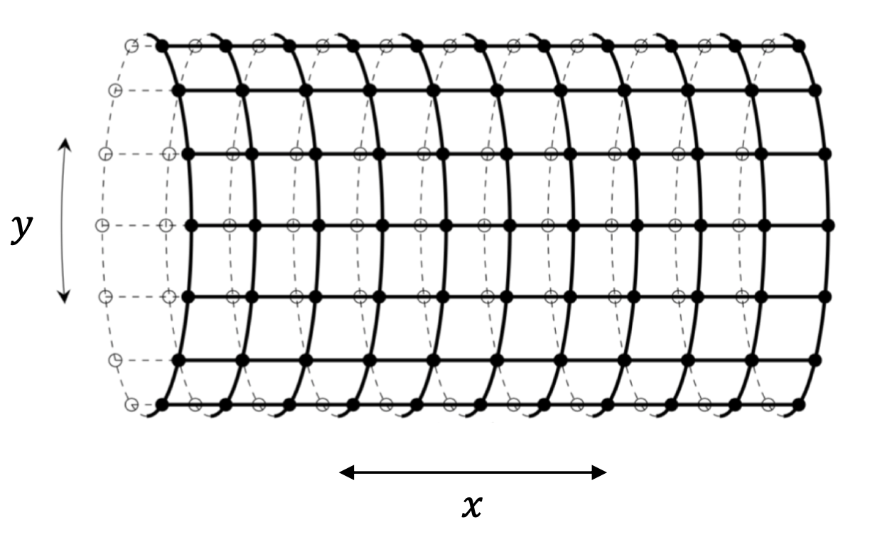
Figure 1: Square lattice with open boundary conditions in the $x-$direction and periodic boundary conditions in the $y-$direction, which resembles a cylinder.

II.2 Boundary conditions and re-initialisation

In this work, we investigate the Abelian Manna Model (AMM) on two-dimensional square lattices, with periodic boundary conditions in the $x-$direction and open boundary conditions in the $y-$direction, Fig. 1. We will call this setup the periodic model. Apart from the periodic boundaries in one direction, the periodic model is identical to the original AMM, which has open boundaries in all dimensions, and they belong to the same universality class (Tab. 9.3 in Huynh, 2013). The periodic boundary condition identifies site $(x,y)$ with site $(x,y+L)$. A set of sites with the same $x$ will be called a ring. The presence of open boundaries in the $x-$direction introduces dissipative transport (Grinstein (1995), Chapter 9.2 in Ref. Pruessner (2012)). Particles added to the system by external driving may leave the lattice through the open boundary after a series of topplings. In fact, particles in the system perform random walks. The average avalanche size $\left\langle s\right\rangle$ can be determined in closed form by mapping it to the expected number of steps of a random walker before escaping from the lattice. In this context and the following, $\left\langle\cdot\right\rangle$ represents the ensemble average of an observable in the stationary state. For a $d$-dimensional square lattice with open boundary conditions in one direction and periodic boundary conditions in other $d-1$ directions, the expected avalanche size is Pruessner (2013)

$$\langle s\rangle=d\frac{(L+1)(L+2)}{12}\ \text{,}$$ (2)

based on the residence time of a random walk. An avalanche leaves behind an array of particles in a quiescent system, that may be thought of as the substrate upon which the next avalanche will be running. Avalanche therefore leaves an imprint on the lattice, such that the substrate particles’ spatial-temporal features are correlated. The expected occupation number $\rho(x,y)$ at site $(x,y)$ in the quiescent state, referred to as the density profile, is defined as $\rho(x,y)=\left\langle z(x,y)\right\rangle$ with sum rule $\sum_{x,y}\rho(x,y)=L^{2}\left\langle\zeta\right\rangle$. The density profile is translational invariant along the $y-$direction due to the periodic boundary conditions, i.e.

$$\forall_{a\in\{1,\ldots,L\}}\rho(x,a)=\rho_{\parallel}(x)\ .$$ (3)

This property does not apply to the $x-$direction, i.e. , generally $\rho(x+a,y)\neq\rho(x,y)$, since translational invariance in the open direction is broken due to the open boundary conditions. In fact, the density profile in the $x-$direction shows a dip towards the open boundaries Willis and Pruessner (2018), because of the transport towards the open ends Paczuski and Bassler (2000). We expect that the density profile has a bearing on the behaviour of the AMM possibly even affecting its critical behaviour, as the density profile immediately affects the particle transport.

We further introduce the connected correlation function

$$\begin{split}C(x_{1},y_{1};x_{2},y_{2})=&\left\langle z(x_{1},y_{1})z(x_{2},y_{2})\right\rangle-\\ &\left\langle z(x_{1},y_{1})\right\rangle\left\langle z(x_{2},y_{2})\right\rangle,\end{split}$$ (4)

which has been measured in Willis and Pruessner (2018) and was found to be surprisingly weak (see Fig. 2 in Willis and Pruessner (2018)). The present work centres around the question whether the weak correlations matter for the critical behavior. To test the effect of correlations of substrate particles, we deliberately destroy them by re-arranging particles between avalanches. If correlations are weak yet important, the critical properties of the Manna Model with the correlations destroyed should differ from those in the periodic model. If correlations are weak and irrelevant, the critical behaviour should remain unchanged. To destroy correlations without unduly changing the density profile and thus tampering with the (critical) behaviours in a “trivial” manner, we introduce four different operations that destroy the correlations of substrate particles while preserving the instantaneous density profile of the substrate. The operation of choice is applied after every non-vanishing avalanche, i.e. , one that has size $s>0$. This is equivalent to applying the operation after every avalanche, even those with non-vanishing size, because only a non-vanishing avalanche can recreate the correlation that are destroyed by the operation. Performing this operation even after vanishing avalanches does not change the substrate particles’ statistics.

Twisting: One method of re-arranging particles is rotating or twisting periodically closed rings of particles in the direction of the periodic boundary condition, by a random angle independently chosen for every ring. To this end, we draw random integer variables $r_{x}$ with $0\leq r_{x}<L$ for each $x\in\{1,2,\ldots,L\}$ and re-initialize the lattice with the configuration $z^{\prime}(x,y)=z(x,y+r_{x})$, subject to the periodic boundary conditions, before the next driving. In other words, after each non-vanishing avalanche, we twist every periodic ring of the lattice independently. Particles within the same ring maintain their relative positions, while particles in neighbouring rings do not. This operation destroys correlations in the open $x-$direction so that after twisting, in a large enough system and assuming finite correlation length, the correlation function asymptotically factorizes, $C(x_{1},y_{1};x_{2},y_{2})\propto\delta_{x_{1},x_{2}}$. If correlations in the substrate are present but irrelevant, then the twisting will not result in a critical behaviour different from the periodic model.

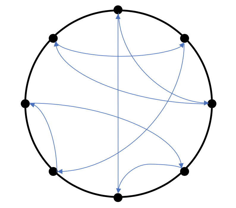
Figure 2: Side view of the periodic AMM with correlations along the $y-$direction destroyed by swapping. The arrows indicate the movement of slabs on the lattice by swapping.

Swapping: The second method destroys correlations in the $y-$direction by randomly swapping slabs cut along the $x-$direction. As illustrated in Fig. 2, we draw new positions $y^{\prime}(y)$ for each $y\in\{1,2,\ldots,L\}$ such that $\{y^{\prime}(1),y^{\prime}(2),\ldots,y^{\prime}(L)\}$ is a random permutation of $\{1,2,\ldots,L\}$ and re-initialize the lattice with the configuration $z^{\prime}(x,y)=z(x,y^{\prime}(y))$ after each non-vanishing avalanche. Again, particle numbers within a ring remain unchanged. Measuring correlations after swapping produces a correlation function that asymptotically factorizes in $y$, $C(x_{1},y_{1};x_{2},y_{2})\propto\delta_{y_{1},y_{2}}$, provided the system is large enough and the correlation length is finite.

Shuffling: The third method, which we call shuffling, destroys correlations in the $x-$direction by re-arranging rings between different systems within an ensemble. Here, ensemble refers to a set of $n$ independent periodic AMMs. In this work, we chose $n=10$. The number $z_{i}(x,y)$ of particles on each site $(x,y)$ now also depends on the index $i\in\{1,2,\dots,n\}$ of the systems. Before shuffling, every system in the ensemble is charged simultaneously and independently, followed by possible avalanches in each system. After every system reaches their quiescent state, for every given $x$, rings of constant $x$ are permutated between the $n$ systems, i.e. , $z_{i}(x,y)$ takes the value of $z_{j}(x,y)$ for all $y$, where $j$ is determined from a random permutation of $\{1,2,\dots,n\}$ for each $x$ independently, as illustrated in Fig. 3. After shuffling, the correlations in the $x-$direction in every system are destroyed.

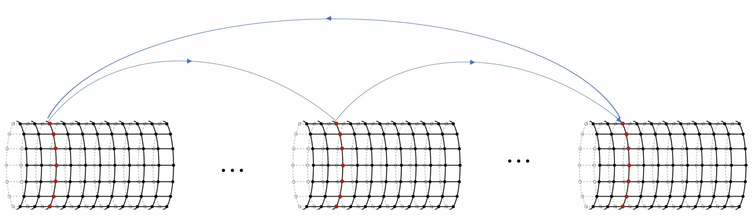
Figure 3: The schematic of the periodic AMM with correlations along the $x-$direction destroyed by shuffling. The arrows indicate the possible movement of rings among different systems by shuffling.

Grinding: The fourth method destroys correlations in both the $x$ and $y-$directions simultaneously by combining twisting and swapping. By twisting, sites lose the correlations to their neighbors in the $x-$direction. By swapping, they lose the correlations to their neighbors in the $y-$direction. As a result, after grinding the correlations in both the $x$ and $y$ directions are destroyed.

III Results

We have performed extensive numerical simulations for the Abelian Manna Model (AMM) in two dimensions with the four operations discussed above. Its scaling behaviour have been characterised by means of moment analysis Tebaldi et al. (1999a); Lübeck (2000), and further validated by data collapses of the probability density functions (PDF) (Chapter 7.4 in Ref. Pruessner (2012)). Large systems with a wide range of sizes have been implemented in this work. For the AMM with twisting, the linear sizes considered were $L\in\{257,513,1025,2049,4097,8193\}$. For the AMM with swapping, shuffling and grinding, due to the higher demands on CPU-time needed to perform the re-arrangement of particles, the largest system size considered was smaller, but not less than $L=2049$. We will present and discuss results for the AMM with twisting in details in the following. Consistent results were found for systems with swapping, shuffling and grinding, presented in Appendix A.

III.1 Moment Analysis

Moment analysis (Chapter 7.3 in Ref. Pruessner (2012)) is a standard technique to extract critical exponents for a quantity $x$ whose probability density distribution (PDF) is assumed to follow the simple finite-size scaling ansatz for $x\gg x_{0}$

$$\mathcal{P}_{x}(x;L)=a_{x}x^{-\tau_{x}}\mathcal{G}_{x}(x/x_{c}(L)),\text{with}\ x_{c}(L)=b_{x}L^{D_{x}},$$ (5)

where $L$ is the system size and $x_{0}$ is the fixed lower cutoff, below which the PDF follows a non-universal function. The two amplitudes $a_{x}$ and $b_{x}$ are non-universal metric factors. Here $x_{c}$ is the upper cutoff above which the PDF deviates significantly from a pure power-law distribution $x^{-\tau_{x}}$ and is dominated by the so-called scaling function $\mathcal{G}_{x}$. Moment analysis is based on the moments

$$\left\langle x^{n}\right\rangle_{L}=\int_{0}^{\infty}\mathcal{P}_{x}(x;L)x^{n}dx\ \text{,}$$ (6)

which according to Eq. (5) behave like De Menech et al. (1998); Christensen et al. (2008)

$$\left\langle x^{n}\right\rangle_{L}\propto L^{D_{x}(1+n-\tau_{x})}+corrections\text{,}$$ (7)

for $n>\tau_{x}$, known as gap scaling. A moment analysis allows the precise determination of the critical exponents $\tau_{x}$ and $D_{x}$, via asymptotic scaling of the moments. The correction terms which scale slower than $L^{D_{x}(1+n-\tau_{x})}$ account for the fact that events of small size $x<x_{0}$ generally do not follow the ansatz in Eq. (5).

The critical exponents for the three avalanche observables considered in this study, avalanche size $s$, avalanche area $a$ and duration time $T$, are extracted using the moment analysis of Eq. (7) and reported in Table 1. The symbols for the critical exponents follow those that are commonly used in the SOC literature, namely $D\equiv D_{s}$, $\tau\equiv\tau_{s}$, $z\equiv D_{T}$ and $\alpha\equiv\tau_{T}$. Since the form of correction in Eq. (7) is a priori unknown, the moments were fitted using the following form with two correction terms, which has proved to work well in a previous analysis Huynh et al. (2011)

$$\langle x^{n}\rangle(L)=a_{1}L^{\mu_{n}}+a_{2}L^{\mu_{n}-1}+a_{3}L^{\mu_{n}-2}\text{.}$$ (8)

The fitting produced a goodness-of-fit at least $q=0.195$ for all observables. We extracted scaling exponents $\mu_{n}$ of the first five moments $n=1,2,\dots,5$ and fitted the resulting values against the linear function $D_{x}(1+n-\tau_{x})$ assuming gap scaling.

The error bar for the exponents extracted in the present work is larger than that reported in one of our earlier studies (Tab. 9.3 in Huynh, 2013) because fewer avalanches are used due to the higher demands on CPU-time needed to perform the re-arrangement of particles on the lattice after every non-vanishing avalanche. Another reason for the larger error bar is the breakdown of simple scaling to be discussed below. In order to reliably reduce finite size effects, we had to simulate systems up to a size of $L=8193$.

Table 1: Critical exponents for the AMM on a two-dimensional square lattice. All moments were fitted using $\langle x^{n}\rangle=a_{1}L^{\mu_{n}}+a_{2}L^{\mu_{n}-1}+a_{3}L^{\mu_{n}-2}$ using $n=1,2,\dots,5$ and critical exponent extracted by fitting them against $D_{x}(1+n-\tau_{x})$ . “$2d$ twisting” refers to the AMM on a two-dimensional lattice closed periodically in one direction and with twisting applied as discussed in Sec. II.2. “$2d$ periodic” refers to the AMM with periodic boundary conditions in one direction but without any operations between avalanches. “$2d$ original” refers to the common AMM on a square lattice open in all directions as studied in Huynh et al. (2011). “MFT” refers to mean-field theory results.

	$2d$ twisting	$2d$ periodic Huynh (2013)	$2d$ original Huynh et al. (2011)	MFT Lübeck (2004)
$D_{a}$	$1.799(7)$	$2.001(1)$	$1.995(3)$	$4$
$D$	$2.028(6)$	$2.763(8)$	$2.750(6)$	$4$
$z$	$1.050(10)$	$1.542(5)$	$1.532(8)$	$2$
$\tau_{a}$	$1.104(11)$	$1.378(2)$	$1.382(3)$	3/2
$\tau$	$1.017(6)$	$1.276(2)$	$1.273(2)$	3/2
$\alpha$	$1.138(26)$	$1.497(8)$	$1.4896(96)$	$2$
$-\Sigma_{a}$	$0.188(19)$	$0.760(4)$	$0.76(2)$
$-\Sigma_{s}$	$0.035(12)$	$0.763(8)$	$0.748(13)$
$-\Sigma_{T}$	$0.145(27)$	$0.766(12)$	$0.73(4)$

The exponents can be combined to produce $\Sigma_{s}=D(1-\tau)$, $\Sigma_{a}=D_{a}(1-\tau_{a})$ and $\Sigma_{T}=z(1-\alpha)$, which are identical under the common assumption of a narrow joint distribution of avalanche size, area and duration Jensen et al. (1989); Christensen et al. (1991); Lübeck (2000); Pruessner (2012).

Table 1 shows a consistent picture, between both the original (four open boundaries) and the periodic (one open and one periodic direction) Abelian Manna Model as well as within each of them as $\Sigma_{a}=\Sigma_{s}=\Sigma_{T}$. In other words, there is no suggestion that closing one of the directions periodically results in a change of exponents in the original AMM. However, the exponents for the AMM with twisting clearly deviate. To start with, $D_{a}$ no longer is close to 2, while $D_{a}=d$ has been observed for $d\leq 4$ Huynh and Pruessner (2012); Bordeu et al. (2019). In fact, all exponents are much reduced. If our operations to destroy correlations had resulted in an effective random neighbour model, we would expect at least some mean field exponents, which are $D_{a}=4$, $D=4$, $z=2$, $\tau_{a}=\frac{3}{2}$, $\tau=\frac{3}{2}$ and $\alpha=2$ Lübeck (2004). However, the exponents we found in the AMM with twisting deviated from the mean field values more than the original AMM. The exponents result in values of $\sum_{x}$ that are inconsistent with the narrow joint distribution assumption.

To validate our numerics, we compare the estimated first moment to Eq. (2) which ought to hold even in the presence of twisting because twisting does not change the distance of any particle to the open boundaries. This produced perfect agreement. Twisting therefore does not have the same effect as bulk-dissipation Barrat et al. (1999)

Similar, consistent results are found for the Abelian Manna Model with swapping, shuffling and grinding, presented in Appendix A, although with larger error bars as smaller system sizes are implemented. All the observables studied are consistent within the statistical error under different operations. This is partially in line with our expectations, as all operations destroy correlations while preserving the instantaneous density profile of the substrate. On the other hand, one may expect correlations in the $x-$direction, as destroyed by twisting and grinding, to have a greater bearing on the scaling behaviour than correlation in the $y-$direction, as destroyed by swapping, shuffling and grinding.

III.2 Probability density functions

In addition to a moment analysis, which extracts the critical exponents from the moments of avalanche observables based on the assumption of simple scaling and gap scaling Tebaldi et al. (1999b); Lübeck (2000), we use the probability density function (PDF) of the observables to qualitatively assess their scaling behaviour in more detail.

Normally, the dependence of the PDFs $\mathcal{P}_{x}(x,L)$ on the system size $L$ is accounted for by the single characteristic scale $L^{D_{x}}$ entering into the scaling function $\mathcal{G}_{x}(x/L^{D_{x}})$, Eq. (5). This function can normally be revealed in a data collapse Pruessner (2012) by plotting $\mathcal{P}_{x}(x,L)x^{\tau_{x}}$ against $x/L^{D_{x}}$, which shows $\mathcal{G}_{x}(x/L^{D_{x}})$ provided $x\gg x_{0}$, the lower cutoff.

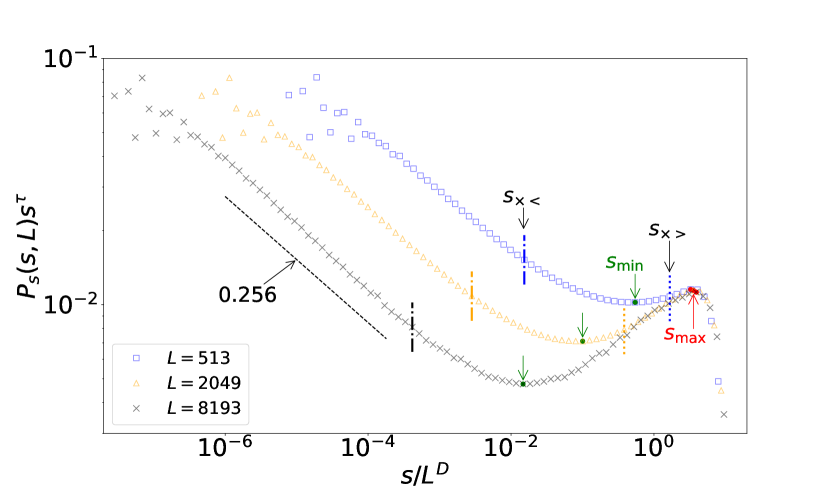
Figure 4: Attempted of a data collapse with $\tau=1.017$ and $D=2.028$, Table 1. Minima are marked by green arrows pointing downwards. Maxima (collapsed together) are marked by the red arrow pointing upwards. Upper and lower crossovers $s_{\times>}$ and $s_{\times<}$ are marked by dotted and dash-dotted lines respectively. The dashed line indicates an apparent exponent of $1.017+0.256=1.273$, the exponent reported for $\tau$ in the original AMM.

Fig. 4 shows an attempted data collapse of the PDF of the avalanche size. Using the exponents found on the basis of the moments in Sec. III.1, Table 1, only a partial collapse can be achieved, which covers only the largest avalanches. This well-collapsed region, starting at around $s_{\times>}(L)$, as shown in Figs. 4 and 5, and terminating at a scale proportional to $s_{\text{max}}$, increases in range on a logarithmic scale, but covers a fraction of events that decreases with $L$, as $s_{\times>}(L)\propto L$, Fig. 5

The apparent power law of the PDF for smaller avalanche sizes is indicated in Fig. 4 by a dashed line, which is characterised by an exponent much closer to the original value, Table 1. Rescaling the PDF as to collapse this region produces the plot shown in Fig. 6. The collapsing region, delimited by a constant lower cutoff $s_{0}$ and the lower crossover $s_{\times<}(L)$ covers an increasing fraction of events, but never the largest. As can be seen in Fig. 5, the lower crossover $s_{\times<}(L)$ scales roughly like the local minimum $s_{\text{min}}$ shown in Fig. 4.

The PDF of the avalanche size thus exhibits two different scaling regimes where the scaling for small and intermediate avalanches follows that with the steeper exponents of the original AMM (Table 1), while larger avalanches follow a flatter distribution with the smaller exponents reported for the AMM with twisting (Table 1). In other words, simple scaling is broken.

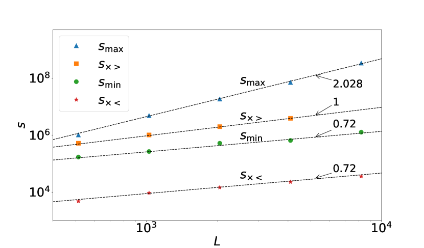
Figure 5: The scaling of $s_{\text{max}}$, $s_{\times>}$, $s_{\text{min}}$ and $s_{\times<}$.

In total we identify four scales in addition to $s_{0}$, namely $s_{\times<}$, $s_{\text{min}}$, $s_{\times>}$ and $s_{\text{max}}$, which according to Fig. 5 scale roughly like power laws of $L$. While $s_{0}$ is constant, $s_{\times<}$ scales approximately like $L^{0.72}$ and is proportional to $s_{\text{min}}$. This is the region governed by the steeper powerlaw of the original AMM. The region from $s_{\times>}\propto L$ to a scale proportional to $s_{\text{max}}\propto L^{2.028}$ is governed by the shallower power law extracted by the moment analysis Sec. III.1 . At very large avalanche sizes, the PDF is shaped by the scaling function $\mathcal{G}(s/s_{c})$ with upper cutoff $s_{c}\propto s_{\text{max}}$. In summary, the PDF of the avalanche size behaves approximately like

$$\mathcal{P}_{s}(s;L)\\ =\begin{cases}f(s;L)&s<s_{0}\\ s^{-1.273}&s_{0}<s<s_{\times<}\propto s_{\text{min}}\propto L^{0.72}\\ s^{-1.017}\mathcal{G}_{s}(s/s_{c})&s_{\times>}\propto L<s\\ &\text{with }\ s_{c}\propto s_{\text{max}}\propto L^{2.028}\end{cases}$$ (9)

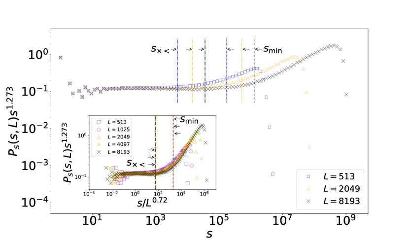
Figure 6: The rescaled histogram of the avalanche size $\mathcal{P}_{s}(s;L)s^{\tau}$, where $\tau=1.273$. $s_{\text{min}}$ and $s_{\times<}$ are marked by dotted and dash-dotted lines respectively. The inset is the same data but shifting the curves vertically by $L^{0.72}$.

Fig. 4 and the inset of Fig. 6 demonstrate that the data in different regions can individually be collapsed according to Eq. (9), but never simultaneously for all avalanche sizes. The majority of events have a size less than $s_{\times<}$, where the scaling exponent $\tau$ is close to that of the original AMM. In other words the majority of events is not affected by the destruction of correlations due to twisting. The moments measured in Sec. III.1 on the other hand are dominated by the scaling of the largest events for any moment $n>\tau-1$, Pruessner (2012), and therefore “report” the exponents characterising the PDF in this region. The situation is very similar to that of the Forest Fire Model Pruessner and Jensen (2002); Grassberger (2002); Pruessner and Jensen (2004), i.e. , twisting breaks simple scaling as it affects only the largest avalanches. Other observables, such as the avalanche area and duration, display similar behaviour, Fig. 7(a) and Fig. 7(b). However, those observables do not display a collapse as clear as that for the avalanche size, Fig. 4.

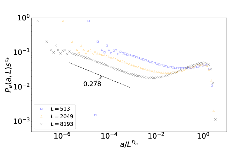
(a) Attempted data collapse of the avalanche area with $\tau_{a}=1.104$ and $D_{a}=1.799$, using the exponents from Table 1. The line indicates an apparent exponent of $1.104+0.278=1.382$, the exponent reported for $\tau_{a}$ in the original AMM.

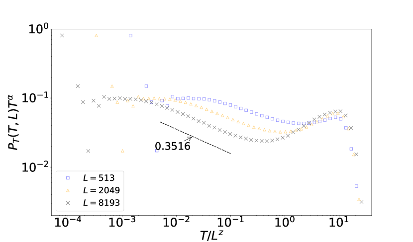
(b) Attempted data collapse of avalanche duration with $\alpha=1.138$ and $z=1.050$, using the exponents from Table 1. The line indicates an apparent exponent of $1.138+0.3516=1.4896$, the exponent reported for $\alpha$ in the original AMM.

Figure 7: Data collapses of avalanche area and avalanche duration .

The scaling behaviour suggested in Eq. (9) can be used to collapse the data in an exotic way, Fig. 8. The “switch” from the scaling $\mathcal{P}_{s}(s;L)\propto s^{-1.273}$ up to $s_{\text{min}}\propto L^{0.72}$, to $\mathcal{P}_{s}(s;L)\propto s^{-1.017}\mathcal{G}_{s}(s/L^{2.028})$ from around $s_{\times>}\propto L$ is implemented by the exponential $\exp{(-A\cdot s/L)}$ where $A$ is a constant chosen to be $0.005$ here. We have experimented with other sigmoid functions, which produce similar results. In particular, the apparent non-monotonicity of the $x$-axis can be cured for the range of $s$ and $L$ considered.

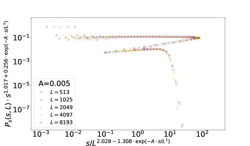
Figure 8: Data collapse using an exponential function which triggers the “switch” from the scaling for small avalanches to that of larger avalanches.

IV DISCUSSION

IV.1 Different exponents

The moment analysis of Sec. III.1 (Table 1) produce exponents for the AMM with twisting that are different from those of the periodic AMM and the original AMM. All exponents, even $D_{a}$, which is generally expected to be identical to the spatial dimension of the lattice Lübeck (2004); Pruessner (2012) are observed to be significantly smaller in the model with twisting. The other operations to destroy correlations, namely by swapping, grinding and shuffling, as described in Sec. II.2, produce moments whose exponents are consistent with the results for twisting, Table 2. This indicates that there is universality underpinning a “decorrelated AMM”.

On the other hand, in Sec. III.2 it was demonstrated that the PDF of the avalanche size and, similarly, for the avalanche duration and area, shows two distinct scaling regimes, as was summarised in Eq. (9). This is because the moment analysis is sensitive only to the scaling of the largest events and therefore reports only the scaling exponents in this region. The situation is similar to that in the Drossel-Schwabl Forest Fire Model, which shows systematic,“clean” scaling exponents in a moment analysis and yet distinct scaling regimes in the PDF Pruessner and Jensen (2004). What makes the Forest Fire Model different from the present AMM with twisting is the remarkably clean collapse of the PDF of the largest avalanche sizes in the latter, Fig. 4, compared to the rather poor collapse of the PDF in the former Pruessner and Jensen (2004) (Fig. 17).

As shown in Sec. III.2, Figs. 4 and 7, the apparent exponents Christensen et al. (2008) characterising the PDFs of the size, area and duration of small avalanches, $\tau$, $\tau_{a}$ and $\alpha$ respectively, are consistent with those found in the original model, Table 1, albeit less clearly so for area and duration. The majority of events occurs in this small and intermediate regime.

We thus arrive at the following picture: The AMM with twisting has two different scaling regimes. Small avalanches display a scaling, characterised by the exponents $\tau$, $\tau_{a}$ and $\alpha$, that are consistent with the original model. Large avalanches in the model with twisting display a scaling with modified exponents. Not only the exponents $\tau$, $\tau_{a}$ and $\alpha$ that normally determine the slope of the PDF are affected, but also the cutoff exponents, $D$, $D_{a}$ and $z$. As far as the regime of large avalanches is concerned, all exponents are clearly reduced, Table 1. The values are inconsistent with the assumption of a narrow joint distribution, Sec. III.1, as is indicated by the different values of $\Sigma_{x}$ in Table 1.

IV.2 Role of correlations

Attributing the results above to the destruction of correlations by the twisting, small avalanches, and thus the majority of events, appear to be much less affected by the “decorrelation” than large avalanches. This is a surprising outcome, as one may expect that large avalanches are not affected by a change in the spatial correlations, based on the following arguments: Firstly, the spatial correlations in the substrate are rather weak. In Willis and Pruessner (2018), the amplitude of the correlations is found to be convergent in the limit of large system size, implying that the correlations do not increase in larger systems. Secondly, during a large avalanche, the substrate is rearranged many times, as many sites topple an increasing number of times during avalanches, which can be seen by $s\geq a$ generally and similarly for the cutoffs of size and area, $L^{D}\gg L^{D_{a}}$ in large $L$, so that the characteristic number of topplings per site taking part diverges with the system size and in fact scales like $L^{D-D_{a}}$ for the largest avalanches, with $D-D_{a}=0.762(9)$ for the periodic model and $D-D_{a}=0.229(13)$ for the AMM with twisting according to Table 1. This suggests the characteristics of large avalanches are generally determined by the dynamics, not by the substrate.

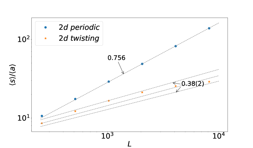
Figure 9: Estimate of the average number of topplings, $\langle s\rangle/\langle a\rangle$, for a range of system sizes. This ratio is always larger in the periodic model, compared to the AMM with twisting. The exponents indicated are $D(2-\tau)-D_{a}(2-\tau_{a})$, which are $0.756(9)$ for the periodic model and $0.38(2)$ for the AMM with twisting based on Table 1, as $\left\langle s\right\rangle\propto L^{D(2-\tau)}$ and $\left\langle a\right\rangle\propto L^{D_{a}(2-\tau_{a})}$.

The average number of topplings per site across all avalanches is shown in Fig. 9 in the form $\left\langle s\right\rangle/\left\langle a\right\rangle$. This ratio should scale with exponent $D(2-\tau)-D_{a}(2-\tau_{a})$, which according to Table 1 is $0.756(9)$ for the periodic model and $0.38(2)$ for the AMM with twisting. The small value of the exponent for the latter explains to some extent the clearly visible corrections, that the AMM with twisting is suffering from. For the largest system sizes considered, even on average, every site topples tens of times during a single avalanche.

A more conservative estimate of the mean ratio $\left\langle s/a\right\rangle$ gives the scaling $L^{D(2-\tau)-D_{a}}$ and thus a constant, assuming $a\sim s^{\frac{D_{a}}{D}}$ based on narrow joint distributions, as well as $\left\langle s\right\rangle\sim L^{2}$ and $D_{a}=2$. Given that $s/a$ frequently vanishes, a finite $s/a$ is indicative of large values of $s/a$ for large avalanches.

From the two points above one might expect that in the periodic AMM a build-up of correlations in the substrate affects the majority of avalanches from event to event, except for the very large events that create “their own environment”. Destroying these correlations should therefore affect small avalanches more than large ones.

However, this turns out not to be the case. In fact, the opposite happens: Small avalanches seem almost unaffected by the twisting, while large avalanches clearly are. Why does this happen? We dismiss the naïve explanation that large avalanches are system-spanning, and thus more affected by the absence of correlations than small avalanches, as every avalanche takes place on a decorrelated substrate. The fraction of sites that are charged only once or topple only once is generally larger for small avalanches than for large avalanches. Again, the destruction of correlations in the substrate should therefore affect smaller avalanches more than larger ones.

We speculate that a more subtle effect is at work. As can be seen in Fig. 2 in Willis and Pruessner (2018), site-occupation shows weak anti-correlations, which means that occupied sites effectively repel occupied sites. As twisting destroys these anti-correlations, activity spreads more easily to occupied nearest neighbours so that large avalanches are triggered prematurely. This is corroborated by the significant reduction of the exponent $D$ characterising the cutoff of the avalanche size distribution. Avalanches in the AMM with twisting are uncharacteristically small. In fact $D$ barely exceeds $d=2$, although it still exceeds $D_{a}$.

The largest avalanches in the decorrelated AMM with twisting are thus small compared to those in the original model. Those very large ones, that take place in the original model, are effectively suppressed in the AMM with twisting because the system is more frequently flushed of fuel and we end up exploring the Manna Model in a regime that would otherwise be considered as sub-critical. The resulting PDF may thus be considered as the PDF of the periodic AMM cut off at around $s_{\times<}$ and characterised in the tail by an interplay of the residual correlations and the dynamics, which produces avalanches that are barely system spanning, $D_{a}<2$ and $D$ barely exceeding $2$.

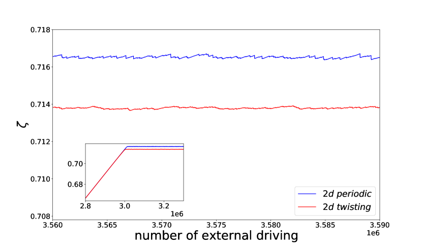
Figure 10: The instantaneous particle density as a function of the number of external driving in a $2049\times 2049$ system. The inset shows the same data but on a lager scale of the number of external drivings.

To illustrate this more vividly, we show the instantaneous particle density in a single realisation as a function of the number of external drivings in a $2049\times 2049$ system in Fig. 10. As shown in the inset, the instantaneous particle density in the AMM with twisting follows that of the periodic model but saturates earlier. As can be seen in the main panel, the substrate density of $\zeta=0.71383(6)$ in the AMM with twisting is typically much lower than that in the periodic model, $\zeta=0.71652(6)$ , amounting to about $11294$ particles “missing” in the former.

The fluctuations of the density are visibly stronger in the periodic model compared to the AMM with twisting, $\sigma(\zeta)=6.07\cdot 10^{-5}$ versus $\sigma(\zeta)=5.69\cdot 10^{-5}$. Yet, they are orders of magnitude smaller than the difference between the two densities of $2.69\cdot 10^{-3}$. The periodic model also has more rugged density fluctuations which display sharp, sudden drops as the very largest of avalanches occur, ejecting many particles from the system at once. We speculate that the AMM with twisting is thus maintained in a subcritical state, so that reducing the correlations effectively cuts off critical scaling at $s_{\times<}$, Sec. III.2.

V Conclusion

In this work, we investigate the role of spatial correlations in the substrate in the Abelian Manna Model (AMM) by destroying them deliberately and observing the change of the critical behaviour. Several operations, twisting, swapping, shuffling and grinding, are performed in extensive numerical simulations of several different systems sizes. Using moment analysis, we extract critical exponents for different observables, namely avalanche size, area and duration, and show that the destruction of correlations in the substrate results in scaling that differs from the periodic Abelian Manna Model. Further assessing the PDFs shows that a crossover takes place from one scaling regime that resembles the periodic AMM to another, new one, that is characterised by the exponents extracted from the moment analysis. The existence of two distinct scaling regimes is reminiscent of the Forest Fire Model Pruessner and Jensen (2002).

Destroying correlations in the Manna Model thus destroys simple scaling. We conclude that substrate correlations are important in the Manna Model, in line with the narrative that the correlated debris left behind by one avalanche shapes the next Watkins et al. (2016), producing non-trivial correlations between and within avalanches Garcia-Millan et al. (2018). Any theoretical treatment will thus need to incorporate these correlations.

In future work, one might study the effects of re-arrangements of substrate particles in other, related models. For example, neural networks have been studied intensely from the perspective of self-organised critical phenomena Hopfield (1994); de Arcangelis et al. (2006); Michiels van Kessenich et al. (2016); Jensen (2021). It has been found experimentally that the connection map in neural network can change over short and long time scales Finnerty et al. (1999); Bennett et al. (2018); Chklovskii et al. (2004); Ko et al. (2013), which effectively destroys the correlations in the substrate and thus strongly affects the system’s behaviour.

Appendix A Moment Analysis of AMM with swapping, grinding, and shuffling

In this section, we report the results of the moment analysis for the AMM with swapping, grinding, and shuffling applied as discussed in Sec. II.2. The linear sizes considered for swapping and grinding operations were $L\in\{257,513,1025,2049,4097\}$. Due to the higher demands on CPU-time needed to perform the shuffling operation, the linear sizes considered for shuffling operations were $L\in\{129,257,513,1025,2049\}$. For this form of destroying the correlations, we were able to fit the critical exponents only for the avalanche size with reasonable goodness-of-fit. The resulting exponent for $\tau$ has an estimated value below unity, which is known to be impossible Christensen et al. (2008), although unity is covered by the error bar.

Table 2: Critical exponents and particle density for the AMM under various operations on a two-dimensional square lattice. All moments were fitted using $\langle x^{n}\rangle=a_{1}L^{\mu_{n}}+a_{2}L^{\mu_{n}-1}+a_{3}L^{\mu_{n}-2}$ using $n=1,2,\dots,5$ and critical exponent extracted by fitting them against $D_{x}(1+n-\tau_{x})$ . “$2d$ swapping”,“$2d$ grinding” and “$2d$ shuffling” refer to the AMM on a two-dimensional lattice closed periodically in one direction and with decorrelating operation applied as discussed in Sec. II.2. “$2d$ periodic” refers to the AMM with periodic boundary conditions in one direction and without any operations between avalanches. “$2d$ original” refers to the AMM on a square lattice open in all directions as studied in Huynh et al. (2011). The goodness-of-fit is at least $q=0.204$ for all observables considered for swapping, at least $q=0.224$ for grinding and $q=0.12$ for shuffling, in which case exponents were extracted only for the avalanche size distribution. The data for twisting, also shown in Table 1 is shown for comparison.

	$2d$ swapping	$2d$ grinding	$2d$ shuffling	$2d$ twisting	$2d$ periodic Huynh (2013)	$2d$ original Huynh et al. (2011)
$D_{a}$	$1.827(48)$	$1.781(21)$	—	$1.799(7)$	$2.001(1)$	$1.995(3)$
$D$	$2.034(17)$	$2.038(15)$	$2.016(40)$	$2.028(6)$	$2.763(8)$	$2.750(6)$
$z$	$1.030(32)$	$1.015(40)$	—	$1.050(10)$	$1.542(5)$	$1.532(8)$
$\tau_{a}$	$1.149(57)$	$1.096(29)$	—	$1.104(11)$	$1.378(2)$	$1.382(3)$
$\tau$	$1.021(14)$	$1.018(13)$	$0.977(36)$	$1.017(6)$	$1.276(2)$	$1.273(2)$
$\alpha$	$1.100(82)$	$1.08(10)$	—	$1.138(26)$	$1.497(8)$	$1.4896(96)$
$-\Sigma_{a}$	$0.273(105)$	$0.171(51)$	—	$0.188(19)$	$0.760(4)$	$0.76(2)$
$-\Sigma_{s}$	$0.042(28)$	$0.036(27)$	$-0.047(72)$	$0.035(12)$	$0.763(8)$	$0.748(13)$
$-\Sigma_{T}$	$0.103(84)$	$0.08(10)$	—	$0.145(27)$	$0.766(12)$	$0.73(4)$