Gravitational memory signal from neutrino self-interactions in supernova

Abstract

Neutrinos with large self-interactions, arising from exchange of light scalars or vectors with mass $M_{\phi}\simeq 10{\rm MeV}$, can play a useful role in cosmology for structure formation and solving the Hubble tension. It has been proposed that large self-interactions of neutrinos may change the observed properties of supernova like the neutrino luminosity or the duration of the neutrino burst. In this paper, we study the gravitational wave memory signal arising from supernova neutrinos. Our results reveal that memory signal for self-interacting neutrinos are weaker than free-streaming neutrinos in the high frequency range. Implications for detecting and differentiating between such signals for planned space-borne detectors, DECIGO and BBO, are also discussed.

I Introduction

Even before the observation of neutrinos from the supernova SN1987A [1, 2], it has been recognised that core-collapse supernova, which produces a high density of neutrinos, would be ideal for the study of neutrino self-interactions ($\nu$-SI) [3, 4, 5, 6, 7, 8, 9, 10, 11, 12, 13, 14, 15, 16, 17, 18, 19, 20, 21, 22, 23]. Among various properties of neutrino, $\nu$-SI mediated by light scalars or vectors are of interest for both laboratory and cosmological applications [24]. $\nu$-SI with scalar or vector mediators as light as $M_{\phi}\sim 10$ MeV can have useful applications in cosmology, and are allowed by neutrino experiments and CMB observations [25, 26, 27]. SI of massive neutrinos reduces the free-streaming length and can be detected in CMB and large-scale structure observation. Moreover, this leads to a modification in the allowed ($n_{s}$, $r$) parameter space of inflationary models [28, 29]. Flavour specific $\nu$-SI can alleviate the $H_{0}$ tension [30, 31, 32, 33], while being allowed by collider constraints [34]. High energy neutrinos can be scattered or absorbed by the cosmic neutrino background and produce a dip in the observations of neutrino spectrum at IceCube which will be a signal of $\nu$-SIs [35, 36, 37, 38].

On the question of the effect of $\nu$-SI on the neutrino signal from core-collapse supernova there is no universal consensus. In the particle picture, one assumes that SIs would lead to successive scatterings of the emitted neutrinos, which in case of large $\nu$-SI, could lead to neutrino trapping and a reduction in the observed flux [5, 39]. In [9], it was shown that interacting neutrinos act as a fluid with sub-luminal velocities for a certain distance, beyond which they free-stream at luminal velocities. Taking motivation from this, the authors in [19] have studied the effect of $\nu$-SI on supernova neutrino signal. They argued that for large SIs in a burst model the duration of the neutrino signal is prolonged compared to the standard neutrino interaction. Following this study, Fiorillo et al. [22, 23] have argued that the more likely scenario for $\nu$-SI in supernova is a steady emission of neutrino from the proto-neutron star (PNS) surface which propagates as a pressure wave with velocity $\sim 1/\sqrt{3}$ close to the PNS surface and increases to unity at the point where the neutrinos start free-streaming. In this steady wind model, despite the presence of SIs, the observable neutrino signal (i.e. the neutrino flux at the detector and the duration of the neutrino signal) remains close to the case of SM-neutrinos, signifying that neutrino observations from supernova do not have a robust signature of SIs in neutrinos.

In order to check for the signatures of $\nu$-SI arising in such scenarios, we examine the gravitational waves sourced by the supernova neutrinos. It has long been pointed out that null-fluids like gravitons emitted from inspiraling binaries [40, 41] or neutrinos from supernova [39, 42, 43] can be a source of gravitational waves and gives rise to a step-function like memory effect in the observed GW signal (For more recent works look at [44, 45, 46]). We compute the memory signal generated by self-interacting neutrinos after they are emitted from the PNS surface. In a region between the radii $R_{s}<r<R_{fs}$ where $R_{s}\sim 10$ km is the PNS radius and $R_{fs}$, known as the free-streaming radius, is the value at which the neutrinos do not suffer any scattering and begin free-streaming. We find that when neutrinos deviate from luminal velocities in the region $R_{s}<r<R_{fs}$ the gravitational memory signal they produce become significantly weaker, yet detectable from the case when there is no $\nu$-SI. Thus, our article serves as a proof-of-principle for probing $\nu$-SI using gravitational wave memory.

The organization of the paper is as follows. In Sec. II, we discuss the $\nu-$SI model analyzed in the paper and the gravitational radiation produced by these sources. In Sec. III, we compute the memory waveform in time-domain. Section IV deals with the detection prospects of the memory signal involving $\nu$-SI. Finally we conclude summarizing our results in Sec. V. An appendix is provided at the end of the paper providing the derivation of the memory time domain formula for relativistic point particles, relativistic fluids and null fluids in time-domain.

II Supernova neutrino physics: Self-interaction and gravitational radiation

This section we describe the basic framework of the paper. We first describe the self-interaction physics of supernova neutrinos and then finally study the gravitational radiation emitted in such systems.

II.1 Neutrino-self interaction in supernova

We study neutrino self-interactions of Majorana neutrinos of the form

$${\cal L}=-\frac{1}{2}g\nu^{T}\nu\phi$$ (1)

which can arise in Majoron models [47, 48] in which lepton number is broken spontaneously and where $\phi$ is the pseudo Nambu-Goldstone boson with a small mass which can be as low as $M_{\phi}\simeq 10$ MeV. The scalar exchange gives rise to a four-Fermi interaction at a scale lower than $M_{\phi}$ with a coupling $G^{\prime}=g^{2}/M_{\phi}^{2}$ which can be many orders of magnitude larger than the Fermi constant of weak interaction $G_{F}$. Neutrinos emitted from the PNS surface have an average number density $n_{\nu}=10^{36}{\rm cm^{-3}}$ and SI cross section of $\sigma_{\nu\nu}=g^{4}/(4\pi M_{\phi}^{2})$. This will have a mean-free path between SIs given by

$$\lambda_{mfp}=\frac{1}{n_{\nu}\sigma_{\nu\nu}}=16.6\,{\rm km}\left(\frac{10^{-5}}{g}\right)^{4}\left(\frac{M_{\phi}}{10{\rm MeV}}\right)^{2}$$ (2)

Therefore the neutrino-fluid undergoes multiple scattering close to the surface of the PNS and only free-streams at a distance $R_{fs}\gg R_{s}={\rm 10\,km}$ where the density drops sufficiently so that the optical depth becomes less than unity. The radial distance $\ell$ where the neutrinos start can be determined from the optical depth at distance $\ell$

$$\tau(\ell)=\int^{\ell}dr\,n_{\nu}(r)\sigma_{\nu\nu}\,.$$ (3)

The distance where where the optical depth $\tau(\ell=R_{fs})=1$ defines the free-streaming radius. The self-interacting neutrinos from supernova behave as a fluid with radial velocity which varies with distance from the PNS (proto-neutron star) radius $r=R_{s}\simeq 10{\rm km}$ to $r<R_{fs}$ [19, 22]. In this diffusion zone the neutrino fluid has a velocity $v(r<R_{fs})\sim 1/\sqrt{3}$. At $r\geq R_{fs}$ the neutrinos free-steam with the speed of light, $v(r\geq R_{fs})=1$ as shown in Fig. (14) of reference [19]. An analytical expression for $v(r)$ can be found from the solution of the equation [23],

$$v(r)\left(1-v^{2}(r)\right)=\frac{2}{3\sqrt{3}}\left(\frac{R_{s}}{r}\right)$$ (4)

It can be checked that at $r=R_{s}$ , this equation has the solution $v(R_{s})=1/\sqrt{3}$ and for $r\gg R_{s}$, we have $v=1$. In our analysis, we have worked with two values of $R_{fs}$, $10$ km and $10^{5}$ km, i.e. small and large diffusion regions. We will see later in this article how gravitational memory is dependent on the the extent of the diffusion zone.

II.2 Gravitational waves from self-interacting neutrinos

We describe the formalism in which GW radiation is produced due to supernova neutrinos. This radiation carries energy of the neutrinos which contributes to the GW memory signal. Initially, in the diffusion region $R_{s}<r<R_{fs}$, the neutrino is described by a relativistic fluid [19]. In this region, $\nu$-SI is present as the neutrino number density is high. Due to multiple scatterings, the neutrino performs a random walk. The random walk path length ($\lambda_{mfp}\sim 1\,\mu$m) is much smaller compared to the other spatial length scales. As mentioned earlier, the neutrino dynamics can be understood as a perfect fluid moving with a sub-luminal velocity, $v\sim 1/\sqrt{3}$ [19]. The corresponding gravitational perturbation for such a relativistic fluid is derived in Appendix A. We rewrite Eq. (39) for convenience,

$$h^{ij}(t,\vec{x})=\frac{4G}{r}\int dt^{\prime}\,d\Omega^{\prime}\int^{\lambda_{fs}}_{R_{s}}{r^{\prime}}^{2}dr^{\prime}\epsilon(\vec{x}^{\prime},t^{\prime})\frac{v^{i}(\vec{x}^{\prime},t^{\prime})v^{j}(\vec{x}^{\prime},t^{\prime})}{1-\vec{N}\cdot\vec{v}(\vec{x}^{\prime},t^{\prime})}\delta\left(t^{\prime}-(t-r)\right).$$ (5)

After emerging from the diffusion region, neutrinos free-stream ($v=1$) in the region $R_{fs}\leq r<\infty$. The radiated gravitational waves as given by the null-fluid expression in Eq. (42),

$$h^{ij}(t,\vec{x})=\frac{4G}{r}\int dt^{\prime}\,d\Omega^{\prime}\int_{R_{fs}}^{\infty}{r^{\prime}}^{2}dr^{\prime}\epsilon(\vec{x}^{\prime},t^{\prime})\frac{{n^{\prime}}^{i}{n^{\prime}}^{j}}{1-\vec{N}\cdot\vec{n^{\prime}}}\delta\left(t^{\prime}-(t-r)\right).$$ (6)

Therefore, the total GW radiation from self-interacting supernova neutrinos is the sum of Eqs.(5) and (6),

$$h^{ij}(t,\vec{x})=\frac{4G}{r}\int dt^{\prime}\delta\left(t^{\prime}-(t-r)\right)\,d\Omega^{\prime}\left\{\int^{R_{fs}}_{R_{s}}{r^{\prime}}^{2}dr^{\prime}\epsilon(\vec{x}^{\prime},t^{\prime})\frac{v^{i}(\vec{x}^{\prime},t^{\prime})v^{j}(\vec{x}^{\prime},t^{\prime})}{1-\vec{N}\cdot\vec{v}(\vec{x}^{\prime},t^{\prime})}+\int_{R_{fs}}^{\infty}{r^{\prime}}^{2}dr^{\prime}\epsilon(\vec{x}^{\prime},t^{\prime})\frac{{n^{\prime}}^{i}{n^{\prime}}^{j}}{1-\vec{N}\cdot\vec{n^{\prime}}}\right\}.$$ (7)

In the limit of weakly self-interacting neutrinos $R_{fs}\rightarrow R_{s}$ and we will obtain the standard neutrino memory signal as in [44]. The flux density of the neutrinos radiated from the PNS surface can be written in terms of the neutrino luminosity as,

$$\epsilon(\vec{x}^{\prime},t^{\prime})=\frac{L_{\nu_{i}}(t^{\prime},r^{\prime})}{4\pi{r^{\prime}}^{2}}\alpha(\theta^{\prime},\phi^{\prime}),$$ (8)

where $L_{\nu_{i}}(t^{\prime},r^{\prime})$ is the neutrino luminosity and $\alpha(\theta^{\prime},\phi^{\prime})$ is the anisotropy parameter which describes the angular asymmetry in the neutrino luminosity due to non-spherical collapse of the supernova. The neutrino luminosity is given by [50],

$$L_{\nu_{i}}(t^{\prime},r^{\prime})=\frac{1}{6}\frac{E_{\nu}}{\tau_{\nu}}\exp\left(-\frac{v_{r}t^{\prime}-r^{\prime}}{\tau_{\nu}}\right)\Theta(v_{r}t^{\prime}-r^{\prime})$$ (9)

where $E_{\nu}=3\times 10^{53}$ ergs is the total energy in the explosion, the decay time of the luminosity is $\tau_{\nu}=3\,{\rm sec}$, and $v_{r}$ is the radial velocity of the neutrino fluid.

In order to clearly outline the role of $\nu$-SI we first evaluate Eq.(7) in two limiting cases. In the limit of weak SIs, the free-streaming of the neutrinos starts from PNR at $r=R_{s}$. In this limit the gravitational wave signal reduces to the standard result

$$h^{ij}(t,\vec{x})=\frac{4G}{r}\int dt^{\prime}\delta\left(t^{\prime}-(t-r)\right)\,d\Omega^{\prime}\int_{R_{fs}}^{\infty}{r^{\prime}}^{2}dr^{\prime}\epsilon(\vec{x}^{\prime},t^{\prime})\frac{{n^{\prime}}^{i}{n^{\prime}}^{j}}{1-\vec{N}\cdot\vec{n^{\prime}}}$$ (10)

On the other hand, for strong self interactions the free-streaming will occur at a distance $R_{fs}\gg R_{s}$ (i.e. $R_{fs}\to\infty$) and the signal given by Eq.(7) will be dominated by the first term

$$h^{ij}(t,\vec{x})=\frac{4G}{r}\int dt^{\prime}\delta\left(t^{\prime}-(t-r)\right)\,d\Omega^{\prime}\int^{\infty}_{R_{s}}{r^{\prime}}^{2}dr^{\prime}\epsilon(\vec{x}^{\prime},t^{\prime})\frac{v^{i}(\vec{x}^{\prime},t^{\prime})v^{j}(\vec{x}^{\prime},t^{\prime})}{1-\vec{N}\cdot\vec{v}(\vec{x}^{\prime},t^{\prime})}$$ (11)

Thus, at first, we compute the memory signal entirely without any $\nu$-SI, then we find it for strong $\nu$-SI given in Eq.(11). Finally, we evaluate the memory signal given in Eq.(7). A comparison of these three scenarios would provide pointers in leveraging gravitational memory as a probe for $\nu$-SI.

III Time domain Gravitational memory waveforms

The expressions for obtaining the gravitational memory for null and relativistic fluids have been given in Appendix A. We respectively provide the expressions for the memory integral below for the three scenarios described previously.

III.1 When $\nu$-SI is small

In the limit of weak $\nu$-SI, we find that $R_{fs}=R_{s}$. There is no diffusion region present in the neutrino propagation. Thus, the Majorana neutrinos free-stream after leaving the PNS surface. Assuming the velocity $v_{r}=1$, the expression for the memory integral is detailed below.

$$[h_{ij}^{\text{mem}}(t,\vec{x})]^{TT}=\frac{4G}{r}\int dt^{\prime}\delta\left(t^{\prime}-(t-r)\right)\,d\Omega^{\prime}\int_{R_{s}}^{\infty}{r^{\prime}}^{2}dr^{\prime}\epsilon(\vec{x}^{\prime},t^{\prime})\bigg{[}\frac{{n^{\prime}}^{i}{n^{\prime}}^{j}}{1-\vec{N}\cdot\vec{n^{\prime}}}\bigg{]}^{TT}.$$ (12)

The anisotropy parameter $\alpha(\theta^{\prime},\phi^{\prime})$ needs to be function of angle $\phi^{\prime}$. We take it to be the form, $\alpha(\theta^{\prime},\phi^{\prime})=\alpha\cos^{2}\phi^{\prime}$. Substituting the Eqs. (8) and (9) in Eq. (12) we find,

$$[h_{ij}^{\text{mem}}(t,\vec{x})]^{TT}=\frac{G}{6\pi r}E_{\nu}\,\bigg{(}1-\mathrm{Exp}\bigg{[}-\frac{(t-r)-R_{s}}{\tau_{\nu}}\bigg{]}\bigg{)}\,\mathcal{A}_{ij}$$ (13)

Here $\mathcal{A}_{ij}$ is basically the angular integral. Depending on the two polarizations of the GW radiation, their expressions become,

$$\mathcal{A}_{ij}=\int d\Omega^{\prime}\alpha(\theta^{\prime},\phi^{\prime})\bigg{[}\frac{{n^{\prime}}^{i}{n^{\prime}}^{j}}{1-\vec{N}\cdot\vec{n^{\prime}}}\bigg{]}^{TT}$$ (14)

$$\mathcal{A}_{+}=\int_{0}^{\pi}\sin\theta^{\prime}\,(1+\cos\theta^{\prime})\,d\theta^{\prime}\,\int_{0}^{2\pi}d\phi^{\prime}\,\cos(2\phi^{\prime})\,\alpha\cos^{2}\phi^{\prime}=\alpha\,\pi$$ (15)

$$\mathcal{A}_{\times}=\int_{0}^{\pi}\sin\theta^{\prime}\,(1+\cos\theta^{\prime})\,d\theta^{\prime}\,\int_{0}^{2\pi}d\phi^{\prime}\,\sin(2\phi^{\prime})\,\alpha\cos^{2}\phi^{\prime}=0$$ (16)

We find no memory strain in the cross-polarization. Hence,the memory strain in plus polarization becomes

$$[h_{+}^{\text{mem}}(t,\vec{x})]^{TT}=\frac{G\alpha}{6r}E_{\nu}\,\bigg{(}1-\mathrm{Exp}\bigg{[}-\frac{u-R_{s}}{\tau_{\nu}}\bigg{]}\bigg{)}\Theta(u-R_{s})$$ (17)

We have set $t-r=u$, and at large retarded time $u\to+\infty$, the memory strain yields $h^{\text{mem}}\sim 10^{-21}$. Our estimates are in agreement with the results found in [44].

III.2 When $\nu$-SI is high and the radial velocity is constant

In the opposite regime, i.e. when $\nu$-SI is quite high, the neutrinos after coming out of the PNS encounter a dense environment of other neutrinos. In this approximation, we take the radial velocity of neutrinos to be $v_{r}=\frac{1}{\sqrt{3}}$.

$$[h_{ij}^{\text{mem}}(t,\vec{x})]^{TT}=\frac{4G}{r}\int dt^{\prime}\delta\left(t^{\prime}-(t-r)\right)\,d\Omega^{\prime}\int^{\infty}_{R_{s}}{r^{\prime}}^{2}dr^{\prime}\epsilon(\vec{x}^{\prime},t^{\prime})\frac{v^{i}(\vec{x}^{\prime},t^{\prime})v^{j}(\vec{x}^{\prime},t^{\prime})}{1-\vec{N}\cdot\vec{v}(\vec{x}^{\prime},t^{\prime})}.$$ (18)

Since the radial velocity $v_{r}=\frac{1}{\sqrt{3}}$, we take $v^{i}(\vec{x^{\prime}},t^{\prime})=v_{r}\,{n^{\prime}}^{i}$. Taking the same anisotropy parameter from the previous calculation, we find the memory strain to be,

$$[h_{ij}^{\text{mem}}(t,\vec{x})]^{TT}=\frac{G}{18\pi r}E_{\nu}\,\bigg{(}1-\mathrm{Exp}\bigg{[}-\frac{(t-r)-\sqrt{3}R_{s}}{\sqrt{3}\tau_{\nu}}\bigg{]}\bigg{)}\,\mathcal{B}_{ij}.$$ (19)

The modified angular integral in this case and its solution for the two polarizations are given below.

$$\mathcal{B}_{ij}=\int d\Omega^{\prime}\alpha(\theta^{\prime},\phi^{\prime})\bigg{[}\frac{{n^{\prime}}^{i}{n^{\prime}}^{j}}{1-v_{r}\,(\vec{N}\cdot\vec{n^{\prime}})}\bigg{]}^{TT}$$ (20)

$$\mathcal{B}_{+}=\int_{0}^{\pi}d\theta^{\prime}\,\frac{\sin^{3}\theta^{\prime}}{1-v_{r}\cos\theta^{\prime}}\,\int_{0}^{2\pi}d\phi^{\prime}\,\alpha\cos^{2}\phi^{\prime}\cos(2\phi^{\prime})\,=\frac{\pi\,\alpha}{2}\bigg{[}\frac{2}{v_{r}^{2}}+\frac{\left(1-v_{r}^{2}\right)}{v_{r}^{3}}\log\left(\frac{1-v_{r}}{1+v_{r}}\right)\bigg{]}=1.44\pi\alpha$$ (21)

$$\mathcal{B}_{\times}=\int_{0}^{\pi}d\theta^{\prime}\,\frac{\sin^{3}\theta^{\prime}}{1-v_{r}\cos\theta^{\prime}}\,\int_{0}^{2\pi}d\phi^{\prime}\,\alpha\cos^{2}\phi^{\prime}\sin(2\phi^{\prime})\,=0$$ (22)

Incorporating the expression in Eq.(21), the final memory strain becomes

$$[h_{+}^{\text{mem}}(t,\vec{x})]^{TT}=1.438\,\frac{G\alpha}{36r}E_{\nu}\,\bigg{(}1-\mathrm{Exp}\bigg{[}-\frac{u-\sqrt{3}R_{s}}{\sqrt{3}\tau_{\nu}}\bigg{]}\bigg{)}\,\Theta(u-\sqrt{3}R_{s}).$$ (23)

We find that as $u\to\infty$, $h^{mem}\sim 10^{-22}$. Thus, the signal in case of high $\nu$-SI is one order less than without SI.

III.3 When $\nu$-SI is moderate

When $\nu$-SI is moderate then both the integrals in Eq.(39) needs to be computed. The final $h_{mem}=h_{mem}^{I}+h_{mem}^{II}$ will have two contributions corresponding to the two regions that the neutrino passes through. Region I is where the velocity is $v_{r}=1/\sqrt{3}$ and region II is where it free streams with a speed of unity. The final form for the expressions are given below.

$$h_{+}^{I}=1.438\,\frac{G\alpha}{36r}E_{\nu}\,\,\Theta(u-{\sqrt{3}}R_{s})\bigg{[}\bigg{(}1-\text{Exp}\bigg{[}-\frac{u-\sqrt{3}R_{s}}{\sqrt{3}\tau_{\nu}}\bigg{]}\bigg{)}-\Theta(u-{\sqrt{3}}R_{fs})\bigg{(}1-\text{Exp}\bigg{[}-\frac{u-\sqrt{3}R_{fs}}{\sqrt{3}\tau_{\nu}}\bigg{]}\bigg{)}\bigg{]}$$ (24)

$$h_{+}^{II}=\frac{G\alpha}{6r}E_{\nu}\,\bigg{(}1-\text{Exp}\bigg{[}-\frac{u-R_{fs}}{\tau_{\nu}}\bigg{]}\bigg{)}\Theta(u-R_{fs})$$ (25)

The Heaviside theta functions in the GW strain waveform signify transition from diffusion region to the free-streaming one. As is evident from Fig.(1), there is a transition when the neutrino value changes from $1/\sqrt{3}$ to unity. The transition takes at a later value of $u$ with the increase in the value of $R_{fs}$. This is because a higher value of $R_{fs}$ denotes that the neutrino spends more time in the diffusion region. In all the plots we find the memory rise time in order of 10s. This confirms that detectors like DECIGO, BBO are well-suited to detect this effect as the maximum characteristic strain $h_{c}(f)$ will peak around $\mathcal{O}(10^{-1})$Hz.

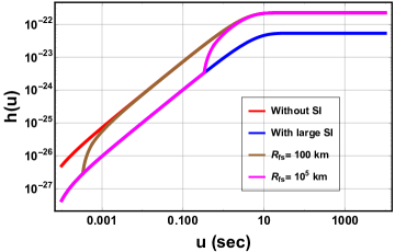
Figure 1: Log-log-plot for the time domain memory strain waveforms. The four waveforms correspond to neutrino propagation without self-interaction (red), with high self-interaction (blue), mixed neutrino propagation with $R_{fs}=100$ km (brown), and $R_{fs}=10^{5}$ km (purple). The plot reveals the build-up of the memory strain along $u$. We find that the amplitude for memory with $\nu$-SI is lower compared to the case when there is no SI ,i.e. when the neutrino free-streams. In cases where there is mixed propagation ($v=1/\sqrt{3}$ when $\nu$-SI is present and $v=1$ in the free streaming region), the waveforms show a transition corresponding to the velocity of the neutrino. With increase in the value of $R_{fs}$, the transition happens at a later $u$-value. The final memory value in all the mixed propagation scenarios is similar to the case when there is no $\nu$-SI. In the plots $\alpha=0.005$ and $R_{s}=10$km.

Similar scenarios can be studied with a smooth profile of neutrino radial velocity, such as, $v_{r}=\sqrt{1-\dfrac{2\,R_{s}^{2}}{3\,r^{2}}}$. In this profile, we find that at $r=R_{S},v_{r}=1/\sqrt{3}$, but at large distances, $v_{r}=1$. Thus, asymptotically the neutrino free streams. We obtain numerically the strain amplitude, $h^{\text{mem}}\sim 4.88\times 10^{-21}$.

IV DETECTION PROSPECTS

This section deals with the possibility of detecting the supernova neutrino memory signals with and without $\nu$-SI discussed previously. In order to achieve this, we first compute the waveforms in frequency domain and then calculate the characteristic strain for such kind of burst profiles.

IV.1 Frequency domain gravitational memory

The frequency domain memory waveforms are used to compare it with the power spectral density (PSD) corresponding to the different detectors. This enables us to understand the possibility of detecting a given signal in the corresponding detector. To this end, we first find the frequency domain waveform. In frequency space, the waveform is given by the expression,

$$|\tilde{h}(f)|=\int h(u)e^{2\pi ifu}\,du.$$ (26)

Incorporating the time domain waveforms from Eqs.(17), (23), (24) and (25) in Eq.(26), we find closed form expressions for the frequency memory signals too. We enlist them below.

$$|\tilde{h}_{1}(f)|=\frac{G\alpha}{6r}E_{\nu}\bigg{|}\pi\delta(2\pi f)+\bigg{(}\frac{i}{2\pi f}+\frac{\tau_{\nu}}{-1+2\pi if\tau_{\nu}}\bigg{)}\text{Exp}[2\pi ifR_{s}]\bigg{|}\,\,\Theta(R_{s}\,^{-1}-2\pi f)$$ (27)

$$|\tilde{h}_{2}(f)|=1.438\,\frac{G\alpha}{36r}E_{\nu}\bigg{|}\pi\delta(2\pi f)+\bigg{(}\frac{i}{2\pi f}+\frac{\sqrt{3}\,\tau_{\nu}}{-1+2\pi if\sqrt{3}\,\tau_{\nu}}\bigg{)}\text{Exp}[2\pi if\sqrt{3}\,R_{s}]\bigg{|}\,\,\Theta((\sqrt{3}R_{s})\,^{-1}-2\pi f)$$ (28)

Eqs.(27) and (28) denote the frequency space memory waveforms for without $\nu$-SI and large $\nu$-SI, respectively. The corresponding Heaviside theta functions in frequency space follows from restriction imposed in the time domain, viz. $u>R_{s}$ in without $\nu$-SI and $u>\sqrt{3}R_{s}$ for large $\nu$-SI. In the final case the neutrino travels (in the diffusion region) from $R_{s}$ to $R_{fs}$ with $v=1/\sqrt{3}$ and for $r>R_{fs}$, it free streams. This is the mixed propagation mode where the $\nu$-SI is moderate.

$$|\tilde{h}_{3}(f)|= 1.438\,\frac{G\alpha}{36r}E_{\nu}\bigg{|}\pi\delta(2\pi f)+\bigg{(}\frac{i}{2\pi f}+\frac{\sqrt{3}\,\tau_{\nu}}{-1+2\pi if\sqrt{3}\,\tau_{\nu}}\bigg{)}\text{Exp}[2\pi if\sqrt{3}\,R_{s}]\bigg{|}\,\,\Theta((\sqrt{3}R_{s})\,^{-1}-2\pi f)$$ (29)

$$-1.438\,\frac{G\alpha}{36r}E_{\nu}\bigg{|}\pi\delta(2\pi f)+\bigg{(}\frac{i}{2\pi f}+\frac{\sqrt{3}\,\tau_{\nu}}{-1+2\pi if\sqrt{3}\,\tau_{\nu}}\bigg{)}\text{Exp}[2\pi if\sqrt{3}\,R_{fs}]\bigg{|}\,\,\Theta((\sqrt{3}R_{fs})\,^{-1}-2\pi f)$$

$$+\frac{G\alpha}{6r}E_{\nu}\bigg{|}\pi\delta(2\pi f)+\bigg{(}\frac{i}{2\pi f}+\frac{\tau_{\nu}}{-1+2\pi if\tau_{\nu}}\bigg{)}\text{Exp}[2\pi ifR_{fs}]\bigg{|}\Theta(R_{fs}\,^{-1}-2\pi f)$$

Frequency domain waveforms are shown in all the these cases in Fig.(2). We observe that similar transition in frequency-space too. With higher values of $R_{fs}$, the diffusion region increases, and the mixed propagation mode transits earlier in frequency space from $v=1$ mode to $v=1/\sqrt{3}$. This is consistent with the results obtained in the time-domain waveforms. This transition feature for mixed neutrino propagation mode is indicator of the $\nu$-SI.

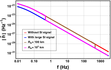
Figure 2: Log-log plot for the frequency domain memory waveforms. These profiles are generated by the fourier transform of the time-domain waveforms. We observe that with the rise in frequency, the velocity of the neutrino in mixed propagation scenarios, becomes equal to $v=1/\sqrt{3}$. The transition happens later for lower values of $R_{fs}$. This is expected since in the time-domain waveforms, a lower value of $R_{fs}$ has a earlier transition.

IV.2 Characteristic strain for neutrino memory waveforms

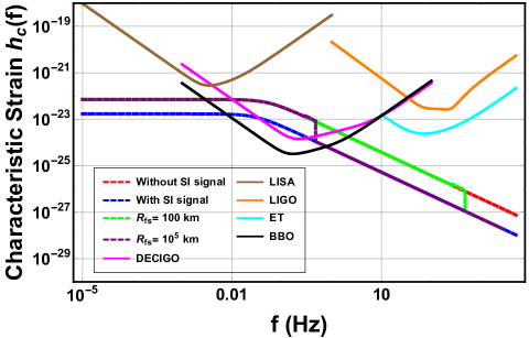
Figure 3: Characteristic strain for the memory signal is plotted along with the characteristic noise of the detectors. The plots show that only DECIGO and BBO are able to detect the memory signal. The transition occurring in $R_{fs}=10^{5}$km can also be detected by BBO and DECIGO. For lower values of $R_{fs}$, i.e. smaller diffusion region, the transition occurs at a higher frequency value which is beyond the sensitivity of the current and future detectors.

In this subsection, we try to compute the characteristic strain and (signal-to-noise ratio) SNR values corresponding to current and upcoming GW detectors. The characteristic strain amplitude $h_{c}(f)$ and its noise counterpart $h_{n}(f)$ are

$$[h_{c}\,(f)]^{2}=4f^{2}|\tilde{h}(f)|^{2}\hskip 56.9055pt[h_{n}(f)]^{2}=fS_{n}(f)$$ (30)

$S_{n}(f)$ denotes the PSD of a detector. We obtain the PSD for detectors like aLIGO, ET, LISA from [51] and, for DECIGO and BBO from [52]. Finally we compute the SNR for memory signals involving $\nu$-SI and provide them in Table-1.

$$(SNR)^{2}=\int_{-\infty}^{\infty}d(\text{log}\,f)\,\frac{[h_{c}\,(f)]^{2}}{[h_{n}(f)]^{2}}$$ (31)

In Fig.(3), we try to analyse the observational potential of the memory signals in some current and upcoming detectors. LIGO, ET, LISA sensitivity curves lie above the characteristic strain of the memory and hence are unable to detect this signal. Only DECIGO and BBO are well-suited to observe this effect of $\nu$-SI. Moreover, we find initially $h_{c}(f)$ is a constant which corresponds to the zero-frequency limit [44, 39, 42]. The transition for lower values of $R_{fs}=100$ km happens at a higher frequency which is beyond the detectability regime of any of these detectors. Nevertheless, we find that for higher values of $R_{fs}$, there is significant potential to detect this signal. The SNR values quoted in Table-I show that detecting the signal without $\nu$-SI and with $\nu$-SI for $R_{fs}$ is similar. For large $\nu$-SI the SNR drops significantly. Thus, as brought out from the analysis, we conclude that the detectors DECIGO and BBO may as well detect this signal since they operate in the range $0.1-10$ Hz.

SNR values
Memory profiles	DECIGO	BBO
Without SI ($v=1$)	3.65	7.88
With SI ($v=1/\sqrt{3}$)	1.40	3.06
$R_{fs}=100$ km	3.65	7.88
$R_{fs}=10^{5}$ km	3.36	7.46

Table 1: The SNR corresponding to the memory profiles for DECIGO and BBO are noted.

V Conclusion

In this article, we have tried to showcase for the first time how large secret $\nu$-SI can lead to significant changes in the gravitational memory profile for a supernova neutrino burst. To this end, we have computed the memory waveforms in both time and frequency domain and have explicitly shown that there exists possibility of detecting such signals using detectors like BBO and DECIGO, thereby enabling our claim.

The basic premise of this article deals with SI of Majorana neutrinos in the Majoron model. In this model, a mediator scalar field having masses of the order of $10$ MeV, gives rise to an effective interaction which is large compared to the weak-interaction scale. Since the coupling is high, the neutrinos coming out of PNS, have smaller mean free paths and, hence, are unable to free-stream. In this region, neutrinos travel as pressure waves with velocity ($v=1/\sqrt{3}$). As the density falls, the neutrino starts free-streaming from $R_{fs}$. A higher value of $R_{fs}$ implies larger diffusion region, leading to stronger interaction and thereby, smaller mean free-path. In our entire analysis, we work with two values of $R_{fs}$, i.e., $100\,$km and $10^{5}\,$km.

We have obtained closed-form expressions for both time-domain and frequency domain memory waveforms. The waveforms are obtained for neutrino burst models with constant anisotropy parameter. In order to ascertain the role of $\nu$-SI vividly, we also analyse two opposite cases– i) where there is no $\nu$-SI; $R_{fs}=R_{s},v_{r}=1$, ii) when the $\nu$-SI is large; $R_{fs}\to\infty,v_{r}=1/\sqrt{3}$. We find that in the time domain, a lesser vale of $R_{fs}$ shows transition earlier from large $\nu$-SI to without $\nu-$SI case. This is because the neutrinos spend less time in the diffusion zone when $R_{fs}$ is small. The frequncy plots, expectedly, shows the opposite behaviour (Fig.(2)). One thing to note is that the transitions in the figures are steep due to the discontinuous nature of the velocity profile we have chosen. In case of smooth velocity profile, the transition will also be smooth. But, the overall feature of the memory waveforms will remain the same.

We find that the detectability of such $\nu$-SI memory signals is achievable with planned space-borne detectors DECIGO and BBO. The transition is observable for large value of $R_{fs}$. For smaller values like $R_{fs}=100\,$km, the signal is indistinguishable from the free-streaming scenario. We require higher detector sensitivities at kHz frequency range.

Finally, to conclude, gravitational wave astronomy holds promise to probe fundamental physics in the strong gravity regime. A more challenging work will be to consider realistic burst models (some of them are given in [44]) and find out the features of this memory signal in those cases. We hope to address these issues in future.

Appendix A Gravitational waves from relativistic fluids

A.1 Relativistic point particles

The stress tensor for massive particles is given by

$$T^{ij}(t^{\prime},\vec{x}^{\prime})=\sum_{a}\gamma_{a}m_{a}v_{a}^{i}v_{b}^{i}\delta^{3}(\vec{x}^{\prime}-\vec{x}_{a}(t^{\prime}))$$ (32)

where $v_{a}^{i}$ is the velocity of the particle labelled ’$a$’ and $\gamma_{a}=(1-v_{a}^{2}){-1/2}$ is the Lorentz factor. Here $\vec{x}_{a}(t^{\prime})$ describes the trajectory of the source particle ’$a$’.

The gravitational waves from the sourced by a stress tensor $T^{ij}$ obey the wave equation

$$\square\,h_{ij}(t,\vec{x})=-16\pi G\,T_{ij}(t,\vec{x}).$$ (33)

The solution of Eq. (33) is of the form

$$h^{ij}(t,\vec{x})=4G\int dt^{\prime}\,d^{3}x^{\prime}\,\,T^{ij}(t^{\prime},\vec{x}^{\prime})\,\cfrac{\delta\left(t^{\prime}-(t-|\vec{x}-\vec{x}^{\prime}|)\right)}{|\vec{x}-\vec{x}^{\prime}|}.$$ (34)

where $\vec{x}^{\prime}$ is the point where the graviton is emitted and $\vec{x}$ is the location of the observer. Substituting from Eq.(32) we obtain

$$h^{ij}(t,\vec{x}) = 4G\int dt^{\prime}\,d^{3}x^{\prime}\,\,\sum_{a}\gamma_{a}m_{a}v_{a}^{i}v_{b}^{i}\delta^{3}(\vec{x}-\vec{x}_{a}(t^{\prime}))\,\cfrac{\delta\left(t^{\prime}-(t-|\vec{x}-\vec{x}^{\prime}|)\right)}{|\vec{x}-\vec{x}^{\prime}|}.$$ (35)

$$= 4G\int dt^{\prime}\,\sum_{a}\gamma_{a}m_{a}v_{a}^{i}v_{b}^{i}\,\cfrac{\delta\left(t^{\prime}-(t-|\vec{x}-\vec{x}_{a}(t^{\prime})|)\right)}{|\vec{x}-\vec{x}_{a}(t^{\prime})|}.$$

The distance of the observer is much larger than the source size, $|\vec{x}|\gg|\vec{x}_{a}(t^{\prime})|$ , take the approximations

$$\delta\left(t^{\prime}-(t-|\vec{x}-\vec{x}_{a}(t^{\prime}))\right) \simeq \delta(t^{\prime}-(t-r+\vec{N}\cdot\vec{x}_{a}(t^{\prime})))$$ (36)

$$= \frac{\delta\left(t^{\prime}-(t-r)\right)}{\frac{d}{dt^{\prime}}(t^{\prime}-(t-r+\vec{N}\cdot\vec{x}_{a}(t^{\prime})))}=\frac{\delta\left(t^{\prime}-(t-r)\right)}{1-\vec{N}\cdot\vec{v}_{a}(t^{\prime})}\,.$$

where $\vec{x}\equiv r\vec{N}$. We also take $\cfrac{1}{|\vec{x}-\vec{x}_{a}(t^{\prime})|}\simeq\cfrac{1}{r}$ and with these approximations after performing the $t^{\prime}$ integral using the delta function, Eq.(35) reduces to the form

$$h^{ij}(t,\vec{x})=\frac{4G}{r}\sum_{a}\gamma_{a}m_{a}\frac{v_{a}^{i}(t_{r})v_{b}^{i}(t_{r})}{1-\vec{N}\cdot\vec{v}_{a}(t_{r})}$$ (37)

where $t_{r}=t-r$.

A.2 Relativistic fluid

For a macroscopic number of particles which source GRW, we go to the fluid limit of the stress tensor which is given by

$$T^{ij}(t^{\prime},\vec{x}^{\prime})=\epsilon(t^{\prime},\vec{x}^{\prime})v^{i}(t^{\prime},\vec{x}^{\prime})v^{j}(t^{\prime},\vec{x}^{\prime})$$ (38)

where $\epsilon((t^{\prime},\vec{x}^{\prime})$ is the energy density and $\vec{v}(t^{\prime},\vec{x}^{\prime})$ the velocity of the fluid element at the spatial location $\vec{x}^{\prime}(t^{\prime})$. A similar derivation as in the previous sub-section gives us the gravitational wave signal in terms of the source as

$$h^{ij}(t,\vec{x})=\frac{4G}{r}\int dt^{\prime}\,d^{3}x^{\prime}\epsilon(\vec{x}^{\prime},t^{\prime})\frac{v^{i}(\vec{x}^{\prime},t^{\prime})v^{j}(\vec{x}^{\prime},t^{\prime})}{1-\vec{N}\cdot\vec{v}(\vec{x}^{\prime},t^{\prime})}\delta\left(t^{\prime}-(t-r)\right).$$ (39)

We can see that Eq.(39) can be derived from Eq.(35) by making the following replacement in going to the fluid limit

$$\sum_{a}\gamma_{a}m_{a}\Rightarrow\int d^{3}x^{\prime}\epsilon(t^{\prime},\vec{x}^{\prime})\,\quad{\rm and}\quad v_{a}^{i}(t^{\prime})\Rightarrow v^{i}(\vec{x}^{\prime}(t^{\prime}))\,.$$ (40)

A.3 Null fluids

For fluids which move at the speed of light with trajectories given by null-geodesics the stress tensor components can be written as

$$T^{ij}(t^{\prime},\vec{x}^{\prime})=T^{00}(t^{\prime},\vec{x}^{\prime}){n^{\prime}}^{i}(t^{\prime},\vec{x}^{\prime}){n^{\prime}}^{j}(t^{\prime},\vec{x}^{\prime})$$ (41)

here ${n^{\prime}}^{i}(t^{\prime},\vec{x}^{\prime})=v^{i}/|\vec{v}|$. With $|\vec{v}|=c=1$, ${n^{\prime}}^{i}$ are components of the unit vector. For a radial flux of mass-less particles as the case of neutrinos from supernova ${n^{\prime}}^{i}=\frac{{x^{\prime}}^{i}}{|\vec{x}^{\prime}|}=(\sin\theta^{\prime}\cos\phi^{\prime},\sin\theta^{\prime}\sin\phi^{\prime},\cos\theta^{\prime})$.

The gravitational signal from radially radiated null-fluids have the form

$$h^{ij}(t,\vec{x})=\frac{4G}{r}\int dt^{\prime}\,d^{3}x^{\prime}\epsilon(\vec{x}^{\prime},t^{\prime})\frac{{n^{\prime}}^{i}{n^{\prime}}^{j}}{1-\vec{N}\cdot\vec{n^{\prime}}}\delta\left(t^{\prime}-(t-r)\right).$$ (42)

where $\epsilon(\vec{x}^{\prime},t^{\prime})=T^{00}(\vec{x}^{\prime},t^{\prime})$ is the energy density of the null fluid.

References

- Arnett et al. [1989] W. D. Arnett, J. N. Bahcall, R. P. Kirshner, and S. E. Woosley, Annual Review of Astronomy and Astrophysics 27, 629 (1989), https://doi.org/10.1146/annurev.aa.27.090189.003213 .
- Chauhan et al. [2021] B. Chauhan, B. Dasgupta, and V. Datar, JCAP 11, 005, arXiv:2106.10927 [hep-ph] .
- Dicus et al. [1983] D. A. Dicus, E. W. Kolb, and D. L. Tubbs, Nuclear Physics B 223, 532 (1983).
- Abbott et al. [2016] B. Abbott et al. (LIGO Scientific, Virgo), Phys. Rev. Lett. 116, 061102 (2016).
- Manohar [1987] A. Manohar, Phys. Lett. B 192, 217 (1987).
- Berezhiani and Vysotsky [1987] Z. G. Berezhiani and M. I. Vysotsky, Physics Letters B 199, 281 (1987).
- Choi et al. [1988] K. Choi, C. W. Kim, J. Kim, and W. P. Lam, Phys. Rev. D 37, 3225 (1988).
- J. A. Grifols, E. Masso, and S. Peris [1988] J. A. Grifols, E. Masso, and S. Peris, Phys. Lett. B (1988).
- Dicus et al. [1989] D. A. Dicus, S. Nussinov, P. B. Pal, and V. L. Teplitz, Physics Letters B 218, 84 (1989).
- Aharonov et al. [1988] Y. Aharonov, F. T. Avignone, and S. Nussinov, Phys. Rev. D 37, 1360 (1988).
- Fuller et al. [1988] G. M. Fuller, R. Mayle, and J. R. Wilson, Astrophys. J. 332, 826 (1988).
- Berezhiani and Smirnov [1989] Z. Berezhiani and A. Smirnov, Physics Letters B 220, 279 (1989).
- Farzan [2003] Y. Farzan, Phys. Rev. D 67, 073015 (2003), arXiv:hep-ph/0211375 .
- Blennow et al. [2008] M. Blennow, A. Mirizzi, and P. D. Serpico, Physical Review D 78, 10.1103/physrevd.78.113004 (2008).
- Heurtier and Zhang [2017] L. Heurtier and Y. Zhang, JCAP 02, 042, arXiv:1609.05882 [hep-ph] .
- Das et al. [2017] A. Das, A. Dighe, and M. Sen, Journal of Cosmology and Astroparticle Physics 2017 (05), 051.
- Shalgar et al. [2021] S. Shalgar, I. Tamborra, and M. Bustamante, Physical Review D 103, 10.1103/physrevd.103.123008 (2021).
- Cerdeñ o et al. [2023] D. Cerdeñ o, M. Cermeño, and Y. Farzan, Physical Review D 107, 10.1103/physrevd.107.123012 (2023).
- Chang et al. [2023] P.-W. Chang, I. Esteban, J. F. Beacom, T. A. Thompson, and C. M. Hirata, Physical Review Letters 131, 10.1103/physrevlett.131.071002 (2023).
- Fiorillo et al. [2023a] D. F. Fiorillo, G. G. Raffelt, and E. Vitagliano, Physical Review Letters 131, 10.1103/physrevlett.131.021001 (2023a).
- Brdar et al. [2023] V. Brdar, A. de Gouvêa, Y.-Y. Li, and P. A. Machado, Physical Review D 107, 10.1103/physrevd.107.073005 (2023).
- Fiorillo et al. [2023b] D. F. G. Fiorillo, G. Raffelt, and E. Vitagliano, Large neutrino secret interactions, small impact on supernovae (2023b), arXiv:2307.15115 [hep-ph] .
- Fiorillo et al. [2023c] D. F. G. Fiorillo, G. Raffelt, and E. Vitagliano, Supernova emission of secretly interacting neutrino fluid: Theoretical foundations (2023c), arXiv:2307.15122 [hep-ph] .
- Berryman et al. [2023] J. M. Berryman et al., Phys. Dark Univ. 42, 101267 (2023), arXiv:2203.01955 [hep-ph] .
- Lancaster et al. [2017] L. Lancaster, F.-Y. Cyr-Racine, L. Knox, and Z. Pan, Journal of Cosmology and Astroparticle Physics 2017 (07), 033.
- Oldengott et al. [2017] I. M. Oldengott, T. Tram, C. Rampf, and Y. Y. Wong, Journal of Cosmology and Astroparticle Physics 2017 (11), 027.
- Kreisch et al. [2020] C. D. Kreisch, F.-Y. Cyr-Racine, and O. Doré , Physical Review D 101, 10.1103/physrevd.101.123505 (2020).
- Barenboim et al. [2019] G. Barenboim, P. B. Denton, and I. M. Oldengott, Physical Review D 99, 10.1103/physrevd.99.083515 (2019).
- Mazumdar et al. [2020] A. Mazumdar, S. Mohanty, and P. Parashari, Physical Review D 101, 10.1103/physrevd.101.083521 (2020).
- Blinov et al. [2019] N. Blinov, K. J. Kelly, G. Krnjaic, and S. D. McDermott, Physical Review Letters 123, 10.1103/physrevlett.123.191102 (2019).
- Blinov and Marques-Tavares [2020] N. Blinov and G. Marques-Tavares, Journal of Cosmology and Astroparticle Physics 2020 (09), 029.
- He et al. [2020] H.-J. He, Y.-Z. Ma, and J. Zheng, Journal of Cosmology and Astroparticle Physics 2020 (11), 003.
- Mazumdar et al. [2022] A. Mazumdar, S. Mohanty, and P. Parashari, Journal of Cosmology and Astroparticle Physics 2022 (10), 011.
- Brdar et al. [2020] V. Brdar, M. Lindner, S. Vogl, and X.-J. Xu, Physical Review D 101, 10.1103/physrevd.101.115001 (2020).
- Ng and Beacom [2014] K. C. Ng and J. F. Beacom, Physical Review D 90, 10.1103/physrevd.90.065035 (2014).
- DiFranzo and Hooper [2015] A. DiFranzo and D. Hooper, Physical Review D 92, 10.1103/physrevd.92.095007 (2015).
- Shoemaker and Murase [2016] I. M. Shoemaker and K. Murase, Physical Review D 93, 10.1103/physrevd.93.085004 (2016).
- Bustamante et al. [2020] M. Bustamante, C. Rosenstrøm, S. Shalgar, and I. Tamborra, Physical Review D 101, 10.1103/physrevd.101.123024 (2020).
- Kolb and Turner [1987] E. W. Kolb and M. S. Turner, Phys. Rev. D 36, 2895 (1987).
- Will and Wiseman [1996] C. M. Will and A. G. Wiseman, Physical Review D 54, 4813 (1996).
- Hait et al. [2023] A. Hait, S. Mohanty, and S. Prakash, Frequency space derivation of linear and non-linear memory gravitational wave signals from eccentric binary orbits (2023), arXiv:2211.13120 [gr-qc] .
- Epstein [1978] R. Epstein, Astrophys. J. 223, 1037 (1978).
- Turner [1978] M. S. Turner, Nature 274, 565 (1978).
- Mukhopadhyay et al. [2021] M. Mukhopadhyay, C. Cardona, and C. Lunardini, JCAP 07, 055, arXiv:2105.05862 [astro-ph.HE] .
- Li et al. [2018] J.-T. Li, G. M. Fuller, and C. T. Kishimoto, Phys. Rev. D 98, 023002 (2018), arXiv:1708.05292 [astro-ph.HE] .
- Yakunin et al. [2015] K. N. Yakunin et al., Phys. Rev. D 92, 084040 (2015), arXiv:1505.05824 [astro-ph.HE] .
- Gelmini and Roncadelli [1981] G. B. Gelmini and M. Roncadelli, Phys. Lett. B 99, 411 (1981).
- Chikashige et al. [1981] Y. Chikashige, R. N. Mohapatra, and R. D. Peccei, Phys. Lett. B 98, 265 (1981).
- Suwa and Murase [2009] Y. Suwa and K. Murase, Phys. Rev. D 80, 123008 (2009), arXiv:0906.3833 [astro-ph.HE] .
- Ko et al. [2022] H. Ko et al., Astrophys. J. 937, 116 (2022), arXiv:2203.13365 [nucl-th] .
- Sathyaprakash and Schutz [2009] B. S. Sathyaprakash and B. F. Schutz, Living Rev. Rel. 12, 2 (2009), arXiv:0903.0338 [gr-qc] .
- Yagi and Seto [2011] K. Yagi and N. Seto, Phys. Rev. D 83, 044011 (2011), [Erratum: Phys.Rev.D 95, 109901 (2017)], arXiv:1101.3940 [astro-ph.CO] .