FATE: Feature-Agnostic Transformer-based Encoder for learning generalized embedding spaces in flow cytometry data

Abstract

While model architectures and training strategies have become more generic and flexible with respect to different data modalities over the past years, a persistent limitation lies in the assumption of fixed quantities and arrangements of input features. This limitation becomes particularly relevant in scenarios where the attributes captured during data acquisition vary across different samples. In this work, we aim at effectively leveraging data with varying features, without the need to constrain the input space to the intersection of potential feature sets or to expand it to their union. We propose a novel architecture that can directly process data without the necessity of aligned feature modalities by learning a general embedding space that captures the relationship between features across data samples with varying sets of features. This is achieved via a set-transformer architecture augmented by feature-encoder layers, thereby enabling the learning of a shared latent feature space from data originating from heterogeneous feature spaces. The advantages of the model are demonstrated for automatic cancer cell detection in acute myeloid leukemia in flow cytometry data, where the features measured during acquisition often vary between samples. Our proposed architecture’s capacity to operate seamlessly across incongruent feature spaces is particularly relevant in this context, where data scarcity arises from the low prevalence of the disease. The code is available for research purposes at https://github.com/lisaweijler/FATE.

1 Introduction

In recent years, a prominent trend in the machine learning landscape has been to design more generic architectures and learning strategies. Examples are multi-modality learning, data modality agnostic learning, or task agnostic learning. Successes in this field can be attributed to the rise of transformer models [32], where (cross-)attention makes the combination of feature-embeddings of different modalities simple, as well as general pre-training and feature extraction methods such as the masked autoencoder (MAE), where training does not depend on data modality or task-specific data augmentations. Yet, those approaches rely on unimodal encoders to process the different types of features corresponding to each data modality.

In this work, we propose a novel architecture, which is agnostic to the number and order of features of the input data by learning a generalized feature space using only one feature-agnostic encoder. We build upon the flexibility of transformers with respect to varying input sequence lengths and ordering. By using a feature encoding similar to the idea of positional encoding and an MAE training strategy, the proposed model learns a general embedding space that captures the relationship between features across data samples. The common way of training an MAE is to mask parts of the input sample, such as patches of an image[12]. In contrast, we propose masking of single feature values to learn the relationship between different features across datasets.

An application, where this characteristic holds significant relevance is the automated processing of Flow Cytometry (FCM) data. An FCM sample is essentially a set of feature vectors (events), each corresponding to a single cell. Based on the properties measured, diverse cell populations can be detected and analyzed. The choice of the features measured and used for analysis is highly task-dependent and often varies even within one use case due to different medical protocols, labs, and routines. While this is no problem for manual analysis, where FCM samples are analyzed one by one, automated processing with e.g. deep learning requires a consistent set of features across datasets.

We evaluate the proposed architecture on the task of cancer cell detection in pediatric Acute Myeloid Leukemia (AML) patients. The proportion of remaining cancer cells during and after treatment, called the Measurable Residual Disease (MRD), is an important factor for risk stratification and the development of effective treatment plans in accordance with individual patients’ needs. This is a particularly challenging task of FCM data analysis, given the possible low proportions (down to $0.01\%$) and high heterogeneity of cancer cells due to patient-specific phenotype characteristics; sample- or patient-specific features are necessary to successfully distinguish healthy from cancerous cells. In addition, training data is scarce because of the low incidence of the disease (5-10 per mio. in Europe[6]). In summary, our contribution is threefold:

1. We introduce a novel architecture FATE (Feature-Agnostic Transformer-based Encoder), which, to the best of our knowledge, is the first one to enable processing of data with flexible input features.

2. We propose a pre-training strategy based on MAE with a novel masking strategy that improves the quality of the representations learned by our model and it is agnostic to the number and type of features of the datasets.

3. Using our proposed pre-training strategy we set a new State of The Art (SOTA) for the task of MRD detection in pediatric AML patients and gain a performance increase of approximately $60\%$ compared to training from scratch.

2 Related Work

In this section, we describe the related work to this paper in different fields: Multimodal deep learning, MAE, and FCM data processing.

Multimodal deep learning

focuses on processing multiple input modalities such as images and text, to learn richer semantic features than unimodal data can offer, as well as for cross-modality tasks such as text-to-image generation. A prominent example is CLIP [26], which is trained on text-image pairs to learn a cross-modality embedding used for different downstream tasks [37, 34]. Another pioneering work in this area is DALL-E [27] for text-to-image generation and several follow-up models. This is also a common practice in the medical field, where it enables the extraction of potentially complimenting features of diverse healthcare data modalities [30, 20, 25, 31]. More recently ImageBind [13] was proposed, which aims at learning a general embedding space for several data modalities such as audio, video, images and text. Those approaches, however, use several unimodal encoders or feature concatenation to process the features related to each modality and therefore expect a fixed number and ordering of features. In contrast, our model allows flexibility with respect to the features used.

Masked autoencoding

has regained attention due to its capacity to learn useful embeddings from unlabelled data serving as an effective pre-training strategy for Deep Learning (DL) models with an increasing number of parameters and capacities. MAE are essentially a general form of denoising autoencoders [33] with a simple idea: mask i.e. remove a part of the input and let the model predict the missing part. This self-supervised training strategy does not depend on data-specific augmentations and is agnostic to the data modality. Starting from its success for natural language models such as BERT[7], it has made its way into vision [12, 9, 36], 3D data processing[38, 14, 16], and many other domains[13, 21, 10, 4]. MAE also has been successfully employed in multimodal learning [4, 11, 5], yet, again they rely on different encoders for each data modality.

Automated FCM data processing

has a wide range of applications in a number of fields and is usually concerned with the detection and classification of novel or targeted cell populations. Early works of targeted cell population detection pool events of different samples from the training set together and train a classifier using pairs of single events and corresponding labels [2, 23, 19]. Methods using single events as input are restricted to learning fixed decision regions, while the relational positioning of cell populations to each other has proven as important information for successfully detecting rare or aberrant cells such as in MRD detection [29]. Therefore, approaches that process a whole FCM sample at once have emerged e.g. using Gaussian Mixture Models [28] or transforming samples to images and applying convolutional neural networks[3]. A more natural solution, without loss of information due to prior transformations are methods based on the attention mechanism [32, 35, 15]. Attention-based models are a way for event-level classification that learns and incorporates the relevance of other cell populations in a sample for the specific task. The current SOTA for automated MRD detection [35] is based on the Set Transformer (ST) [17], an efficient variation of the Transformer model specifically designed for sets. Those approaches assume, however, a fixed set of features during training and inference. FCM data features are highly variable even within one dataset; reducing them to the greatest common intersection for consolidated processing dismisses discriminative information for the successful identification of targeted cells. There exists a work that aims at combining the features of samples by using nearest neighbor imputation[18, 1, 24] but a recent study shows that those methods have severe limitations due to the questionable accuracy of imputed values for downstream analysis[22].

3 Methods

Our feature-agnostic model has a simple architecture depicted as an encoder and a prediction head. The transformer architecture is equivariant to permutations of the input sequence and can handle different sequence lengths. We exploit those properties in two ways. First, to be able to process events with different numbers and ordering of features, and second to be able to process samples with varying amounts of events. Fig. 1 shows the architecture described in Sec. 3.2.

For pre-training of our FATEncoder we use an MAE that is trained to reconstruct the measurement values of masked features. Note that this differs from standard masking where whole instances of the data sample such as patches or pixels of images are masked. An illustration of the proposed MAE is given in Fig. 2, and in Sec. 3.3 its components are explained in detail.

3.1 Preliminaries

Formally, we denote an input sample (set) $\boldsymbol{X}_{i}$ to our model as

$$\boldsymbol{X}_{i}=\{\boldsymbol{x}_{k_{i}}\in\mathbb{R}^{F_{i}}\}_{k_{i}=1}^{n_{i}},$$ (1)

where $F_{i}$ is the dimension of the feature vectors i.e. the number of features, and $n_{i}$ is the number of elements in the input set. One dataset constituted of $N$ samples is a set of sets

$$\{\boldsymbol{X}_{i}\in\mathbb{R}^{n_{i}\times F_{i}}\}_{i=1}^{N}.$$ (2)

In the context of FCM data $\boldsymbol{x}_{k_{i}}$ is one event and $F_{i}$ the features measured by FCM during acquisition. The number of events as well as the feature space can vary between samples; $n_{i}$ is typically between $10^{4}$ and $10^{6}$ and $F_{i}$ between 10 and 20 (limited by the properties of FCM acquisition).

We use standard attention as proposed in [32] taking queries $\boldsymbol{Q}$, keys $\boldsymbol{K}$ and values $\boldsymbol{V}$ as input. For self-attention $\boldsymbol{Q}$, $\boldsymbol{K}$ and $\boldsymbol{V}$ are linear projections of the same input set $\boldsymbol{X}_{i}$, while for cross-attention $\boldsymbol{Q}$ is either a learnable vector or our feature encodings as explained below, $\boldsymbol{K}$ and $\boldsymbol{V}$ are again linear projections of the same input set $\boldsymbol{X}_{i}$.

3.2 FATEncoder

The proposed encoder creates a common embedding space of fixed dimension $F_{c}$, regardless of the number and order of features of the input sample. It can be subdivided into two parts, which we call the Feature-Encoder and the Set-Encoder. The first part is responsible for being able to process inputs with different ordering and number of features, while the second part provides the context of all other events within one sample.

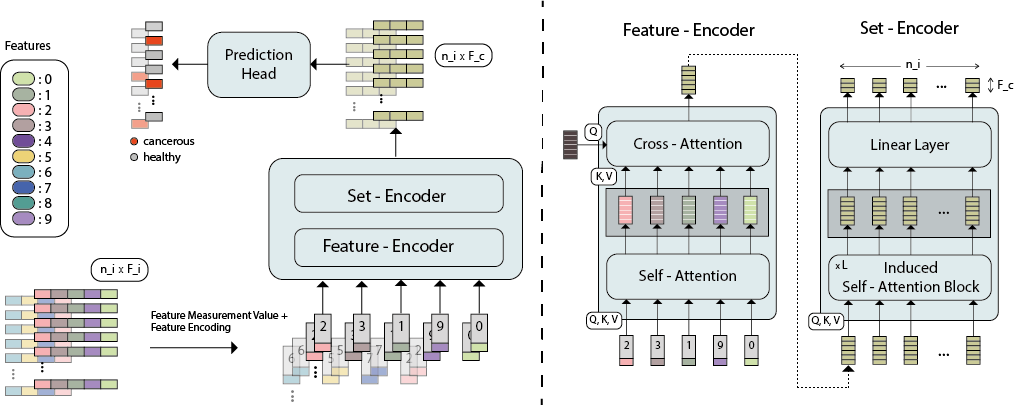
Figure 1: Illustration of the architecture of our model. Left: Each input feature of each event is concatenated with a positional encoding descriptor. These augmented features are updated using the other features of each event (Feature-Encoder) and additional events from the same sample (Set-Encoder). The resulting features, which are independent of the number and type of features used in the input, are used for the final prediction. Right: Detailed illustration of the Feature-Encoder and Set-Encoder networks. We use Self- and Cross-Attention between features in the Feature-Encoder and Induced Self-Attention between events within the sample.

In order to achieve the feature agnostic property, the Feature-Encoder treats the feature values of single events as input sequences, i.e. a sequence of scalar values. Given a sample $\boldsymbol{X}_{i}$, each event $\boldsymbol{x}_{k_{i}}\in\mathbb{R}^{F_{i}}$ thus turns into an input sequence

$$[x_{k_{i_{1}}},\dots,x_{k_{i_{F_{i}}}}]^{\text{T}}\in\mathbb{R}^{1\times F_{i}}.$$ (3)

We employ feature encoding similar to the idea of positional encoding, so the model knows what feature the scalar value in the sequence belongs to, and hence is able to relate them to others and learn their semantic meaning in the context of the dataset. The encoding is concatenated to the scalar measurement value of its corresponding feature, making the final input to our FATEncoder a sequence of vectors

$$\begin{split}[\phi_{E}(\boldsymbol{x}_{k_{i}})_{1},\dots,\phi_{E}(\boldsymbol{x}_{k_{i}})_{F_{i}}]^{\text{T}}\in\mathbb{R}^{1+D_{E}\times F_{i}},\\ \phi_{E}(\boldsymbol{x}_{k_{i}})_{j}\coloneqq[x_{k_{i_{j}}};\boldsymbol{E}_{j}]\in\mathbb{R}^{1+D_{E}},\end{split}$$ (4)

with $\boldsymbol{E}_{j}$ as the feature encoding vector for feature $j$ and $D_{E}$ as its dimension.

Initially, self-attention is applied between those input vectors followed by cross-attention with a learned query vector $\boldsymbol{q}\in\mathbb{R}^{D_{\text{hidden}}}$ that summarizes the information of all features and transforms it into one single embedding vector of fixed dimension $\boldsymbol{z}_{k_{i}}\in\mathbb{R}^{D_{\text{hidden}}}$,

$$\begin{split}\boldsymbol{z}_{k_{i}}=\text{CrossAttn}(\boldsymbol{q},\text{SelfAttn}(\phi_{E}(\boldsymbol{x}_{k_{i}})),\\ \phi_{E}(\boldsymbol{x}_{k_{i}})\coloneqq[\phi_{E}(\boldsymbol{x}_{k_{i}})_{1},\dots,\phi_{E}(\boldsymbol{x}_{k_{i}})_{F_{i}}].\end{split}$$ (5)

After all elements of one sample have passed through the Feature-Encoder, the Set-Encoder puts the event-embeddings $\boldsymbol{z}_{k_{i}}$ of one sample in context to each other. For this we utilize the Induced Self-Attention Blocks (ISABs) as introduced with the ST[17] (see supplementary materials). The ISAB uses learned queries (induced points) to reduce the $\mathcal{O}(n^{2})$ complexity of self-attention to $\mathcal{O}(nm)$ with $n$ denoting the input sequence length and $m$ the number of induced points. Finally, a linear layer maps the embedding to its final embedding dimension $F_{c}$. The Set-Encoder can be summarized as,

$$\{\boldsymbol{z}_{k_{i}}\}_{i}^{n_{i}}\leftarrow\text{LinLayer}(\text{ISAB}^{(l)}(\{\boldsymbol{z}_{k_{i}}\}_{i}^{n_{i}}),$$ (6)

with $l$ being the number of ISAB layers applied.

Feature encoding

In contrast to the positional encoding used in e.g. natural language processing, where ordinal encodings i.e. encodings that have a ranked ordering are used, our feature encoding should be nominal, thus not imposing an artificial relationship between values. A typical choice is one-hot encoding. However, with this choice, the dimension grows with the number of features covered and after training this number is locked-in given that adding new features would increase the dimension of the input vectors. This is why we chose learned encoding vectors of fixed dimension as used in [8] i.e. a learnable function

$$e:\{0,\dots,M-1\}\mapsto\mathbb{R}^{D_{E}},$$ (7)

where $M$ denotes the number of different features present in the training data set.

See supplementary materials for a full list of features used.

Prediction head

As prediction head, we use a 2-layer MLP with GELU as an activation function and a hidden layer dimension equal to the common feature space dimension $F_{c}$.

3.3 FATE-MAE

We propose an MAE strategy for pre-training our model. Like all autoencoders, our method uses an encoder that transforms the observed signal into a latent representation, and a decoder that reconstructs the original signal from this latent representation. However, our encoder is specifically designed to be able to process varying input features as described in Sec. 3.2. Consequently, our decoder has to be able to reconstruct a varying amount of features. The masking strategy and decoder architecture are described in the following; Fig. 2 gives an overview of the MAE. A detailed illustration of our proposed decoder architecture is given in the supplementary materials.

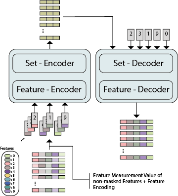
Figure 2: Masked autoencoder strategy used to train our model. During pre-training we mask a set of features for each event. The features remaining after the masking are given as input to our model to be encoded in a unified feature space. A decoder with a symmetric architecture of our encoder is used to predict the masked features in the initial step.

Masking

Contrary to common masking strategies, where full instances e.g. patches of an image are masked, we mask a proportion of feature measurement values per element of the input set $\boldsymbol{X}_{i}$ i.e. per feature measurement vector. The proposed masking strategies allow us to learn the relationship between features in the context of the composition of cell populations within and across samples, in contrast to learning the relationship between cell populations given a fixed set of features, which is standard masking. The strategy is straightforward: We define a fixed ratio of features to mask (i.e. remove); a masking ratio of $0.5$ would mean removing half of the feature measurement values in each feature measurement vector of all samples. What features are to be masked is chosen randomly following a uniform distribution and can be different for each $\boldsymbol{x}_{k_{i}}\in\boldsymbol{X}_{i}$.

Decoder

The decoder is symmetric to the encoder. Following the structure of the encoder, we divide it into the Set-Decoder and Feature-Decoder. The Set-Decoder consists of ISAB layers to capture the relation between the embeddings of one sample $\{\boldsymbol{z}_{k_{i}}\}_{i}^{n_{i}}$. The Feature-Decoder reconstructs the original feature measurement values of each set element $\boldsymbol{x}_{k_{i}}\in\mathbb{R}^{F_{i}}$ from its corresponding embedding vector $\boldsymbol{z}_{k_{i}}\in\mathbb{R}^{F_{c}}$ given the context of all elements in the input set. This is not trivial due to the varying number of features between samples. To achieve this we condition the decoder on the features of which we want their measurement values to be reconstructed by cross-attending their feature encodings with the output of the set-decoder. Finally, similar to the feature-encoder we apply self-attention between the reconstructed feature measurement value vector of each $\boldsymbol{x}_{k_{i}}$ and map them with a linear layer to a scalar value. For a detailed illustration of the proposed decoder see supplementary materials.

4 Experimental Setup

In this section, we give an overview of the experiments conducted, the implementation details, and the datasets used.

We focus on the task of MRD detection of FCM samples in pediatric AML patients given that it is one of the most challenging tasks in FCM data analysis with increased varying features between samples. AML depicts a particularly high heterogeneity of cancer cells in comparison to other sub-types such as b-Cell Lymphoblastic Leukemia (b-ALL). Consequently, the features necessary to successfully separate healthy from cancer cells are highly diverse. In addition, it is a very rare disease resulting in a natural data scarcity. Hence, the ability to use other datasets for pre-training while being flexible with respect to input features is crucial.

We treat the problem as a binary classification, cancerous or healthy, and use binary cross-entropy as loss function for supervised training. Precision $p$, recall $r$, and $F$-score $F_{1}$ with cancer cells as positives are used as evaluation metrics. The metrics are calculated per sample, then averaged to determine the final metrics of the test set.

4.1 Datasets

The main data set (AML-MRD) for the downstream task of MRD detection consists of 71 FCM samples coming from 12 different pediatric AML patients. The samples were collected at different time points during therapy between the years 2021 and 2022. The number of markers used for samples of this dataset varies between 10 and 14. Additionally, the forward- and side-scatter of the laser light, which reflect the physical properties of the cells, are used as features. Between all samples of this dataset, 6 markers are shared. For a full listing of the number of samples per patient and the corresponding features see the supplementary materials.

For pre-training we use data from pediatric b-ALL patients at day 15 of therapy, data from pediatric AML patients at diagnosis, where cancerous cells have replaced most of the healthy cells, as well as FCM samples from screening cases or recovered patients, that are free of cancer cells (MRD negative). The b-ALL data is a publicly available dataset (ALL-MRD) collected from three different laboratories in Berlin, Buenos Aires, and Vienna. The diagnosis (DIA) as well as the MRD negative dataset (CONTROL) are a collection of samples from different laboratories in Vienna, Padua and Essen between the years 2016-2022. CONTROL and DIA have 4 features with AML-MRD in common, while ALL-MRD only has 2 excluding forward- and side-scatter. Supplementary materials give an overview of all features and the overlaps between datasets.

Sampling and research were approved by local Ethics Committees, and informed consent was obtained from patients’ or patients’ parents or legal guardians according to the Declaration of Helsinki. Ground truth was obtained using manual analysis by at least two experts. Whenever available, results were confirmed using an independent molecular methodology (RT-PCR).

The datasets we use for pre-training are not suitable as training data for the downstream task of MRD detection in pediatric AML patients, given the different types of cancer cells (ALL-MRD), composition of data (DIA), or lack of cancer cells (CONTROL). However, they can be successfully utilized for pre-training by our proposed model as we show in Sec. 5.

Tab. 1 provides a tabular overview of the data sets.

Table 1: Description of the FCM data sets used.

Name	City	Years	Samples
AML-MRD	Vie	2021-22	71
CONTROL	Vie, Pad, Ess	2016-21	308
DIA	Vie, Pad, Ess	2016-22	110
ALL-MRD	Vie, Bln, Bue	2009-14	338

4.2 Experiments

We conduct several experiments to evaluate the proposed FATE architecture and MAE. The current SOTA for automated MRD detection in FCM data based on the ST [35] serves as a baseline using the official implementation.

We train the models from scratch and compare them to two different types of pre-training. First, we pre-train the baseline and the FATE model supervised with the CONTROL, DIA, and if applicable ALL-MRD datasets. Second, we test our proposed pre-training method based on MAE using the CONTROL, DIA and ALL-MRD datasets.

Implementation details

For the training-from-scratch experiments, we train our model for 400 epochs and use early stopping after 300 epochs if there is no improvement of the $F_{1}$-score on the validation set. The baseline model is trained for 200 epochs with early stopping after 100 epochs since it showed a tendency to overfit on the small datasets.

For the supervised pre-training we use 1500 epochs and finetune for 100 epochs using the pretained weights as initialization. Given that the task of finetuning is the same as for pre-training we do not remove the prediction head. For pre-training of the baseline we conduct two experiments. First, we only use the 4 features plus forward- and side-scatter that the CONTROL and DIA have in common with the AML-MRD dataset and second, we use the union over all occuring features in all three datasets as input imputing the missing ones with zeros. For the FATE model each input sample’s individual features can be utilized.

Pre-training of the FATE MAE is conducted for 2000 epochs for all experiments and pre-trained weights are again used as initialization for training of the downstream task. The model is finetuned for 300 epochs with early stopping after 200 and different masking-ratios are evaluated.

The $L_{1}$-loss is used and calculated between the true measurement values of masked features and those reconstructed by the decoder. With respect to the learning rate for finetuning and from-scratch experiments, we opt for the cosine-annealing learning rate scheduler with a starting value of $0.001$, a minimum value of $0.0002$, and a maximum of 10 iterations. Throughout all pre-training experiments, we use the same scheduler with a starting value of $0.001$, a minimum value of $0.00002$, and a maximum of 100 iterations. AdamW optimizer is employed for all experiments. A batch size of 32 and 8 is used for pre-training and finetuning, respectively. Training is conducted on an NVIDIA GeForce RTX 3090.

All models are trained at least three times with different initialization and mean and standard deviations are reported.

Patient cross-validation

Since the target dataset AML-MRD is small with 71 samples and several samples can originate from the same patient we employ a cross-validation to maximize the amount of training and evaluation data. The model should be capable of detecting MRD in FCM data of new patients, meaning for a fair assessment, samples taken from one patient must not be split up between the training, evaluation, and test set. Therefore we conducted a “patient-cross-validation”, where each patient generates one split, i.e. the patient’s samples are held out as test data. All remaining samples from other patients are divided into training and evaluation sets with a ratio of $0.8$ and $0.2$, respectively. The reported metrics are the average of the resulting values over all samples. See supplementary materials for a full list of splits and the number of training, validation, and test samples.

Model architecture

For the baseline model we use the same architecture as proposed in [35], namely 4 ISAB layers with a hidden dimension of 32 and 16 induced points. For our FATE model, we use the architecture as described in Sec. 3 with 3 ISAB layers in the encoder and decoder, a hidden dimension of $32$, and an embedding space dimension $F_{c}=8$. The learned feature encodings have a dimension of $D_{E}=10$.

Table 2: Results of our main experiments. We compare our model trained from scratch and pre-trained with different strategies to the current state-of-the-art Set-Transformer model [35]. The results show that our model performs similarly to ST on a supervised setup, but, when pre-trained with additional data, is able to outperform this model by using more data during pre-training.

	Pre-train	Dataset	${p}$	${r}$	${F_{1}}$
ST [35]	-	-	0.385	0.366	0.314 $\pm 0.015$
	Sup.	CON, DIA	0.446	0.356	0.324 $\pm 0.029$
ST [35] (All Features)	-	-	0.328	0.456	0.328 $\pm 0.011$
	Sup.	CON, DIA	0.493	0.436	0.332 $\pm 0.017$
	Sup.	CON, DIA, ALL-MRD	0.457	0.385	0.297 $\pm 0.001$
FATE (Ours)	-	-	0.445	0.435	0.315 $\pm 0.004$
	Sup.	CON, DIA	0.6175	0.401	0.389 $\pm 0.058$
	Sup.	CON, DIA, ALL-MRD	0.531	0.444	0.413 $\pm 0.053$
	Sup.+MAE	CON, DIA, ALL-MRD	0.611	0.550	0.496 $\pm 0.045$

Table 3: Results for different masking ratios of the input features. We can see that a strong masking ratio decreases performance due to the small number of features of each event.

Masking ratio	${p}$	${r}$	${F_{1}}$
$0.75\%$	0.574	0.389	0.363 $\pm 0.004$
$0.5\%$	0.578	0.472	0.459 $\pm 0.016$
$0.25\%$	0.611	0.550	0.496 $\pm 0.045$

5 Results

Tab. 2 shows the results of the experiments conducted. Training from scratch yields similar results for all three setups, ST with the intersection of all features, ST with the union over all features in all datasets, and our FATE model. The ST using all features as input, where missing ones are imputed with $0$, performs slightly better showing the benefit of sample-specific features. Our FATE model needs to learn the feature encoding and the common embedding space, which is hard given the little training set when training from scratch. Yet it holds comparable results with higher mean precision and recall.

Pre-training the models supervised with the CON and DIA dataset improves results for all models. The biggest increase can be seen for our FATE model, indicating that the proposed architecture can successfully learn the relation between features across different samples. Surprisingly, when adding the ALL-MRD dataset to pre-training, the performance of the ST drops. One explanation is the increased difference in features and in cancer cells to be detected since b-ALL is a different leukemia subtype than AML. For our proposed model the performance increases further despite those differences to a mean $F_{1}$-score of $0.413$, which can be interpreted as that the general relationship between markers in the context of the downstream task is extracted and beneficial for the model.

Pre-training with the proposed MAE strategy is only possible for the FATE architecture. We can see that the results further increase to $F_{1}=0.496$, yielding an improvement to approximately $60\%$ over training from scratch. The results indicate that our FATE model can successfully learn a common embedding space and utilize the information of all sample-specific features. Visualizations of the learned embeddings are provided in the supplementary material.

We evaluated different masking ratios for pre-training: $0.25\%$, $0.5\%$, and $0.75\%$. Tab. 3 shows the results for those experiments. We can see that performance increases with a decreasing ratio, where $0.25\%$ yields the best performance. While the performance for a masking ratio of $0.5\%$ is still significantly better than supervised pre-training, when masking with a ratio of $0.75\%$, although still better than training from scratch, performance drops below supervised pre-training due to the small number of features for each event.

6 Conclusion

In this work, we introduce a novel architecture, FATE, that is agnostic to the number and order of features of the input data by learning a generalized feature space using only one feature-agnostic encoder. Further, we propose a pre-training strategy based on MAE which, contrary to standard practices where complete feature vectors are masked during pre-training, masks part of the input features and tries to reconstruct them from the remaining ones. We show that, with this model and pre-training strategy, we are able to leverage new datasets during pre-training and improve current state-of-the-art on FCM data by a large margin.

In the future, we would like to investigate which features are more relevant for feature reconstruction and downstream tasks by analyzing the attention weights of our model, in order to improve future data acquisition. Moreover, we would like to investigate how the quality of the representations is affected by the number of common features during pre-training.

Appendix A Datasets

Tab. 4 gives a detailed overview of the number of patients and their samples collected per dataset, as well as city and years of acquisition. All samples from the datasets used for pre-training (CONTROL, DIA, ALL-MRD) are from different patients than those in the target dataset, AML-MRD, for a fair assessment of generalization between patients.

Table 4: Description of the FCM datasets with respect to the city of the laboratory and the time-span the samples where acquired, the number of samples per dataset as well as the number of patients the samples were taken from.

Dataset	City	Years	Samples	Patients
AML-MRD	Vienna	2021-2022	71	12
CONTROL	Essen	2016	52	17
	Padua	2016-2021	88	22
	Vienna	2016-2021	168	57
DIA	Essen	2016	24	12
	Padua	2016	6	3
	Vienna	2016-2022	80	30
ALL-MRD	Vienna	2009-2014	200	200
	Berlin	2015	72	72
	Buenos Aires	2016-2017	66	66

Fig. 3 shows four different FCM samples of different patients coming from the AML-MRD dataset. The plots are 2D projections of the sample on different features including forward- and side-scatter (see Appendix B). Each point corresponds to the feature measurement vector of one cell. We can see the variation in cancer cells (red) regarding positioning and proportion as well as the variation in density of healthy cell populations (blue).

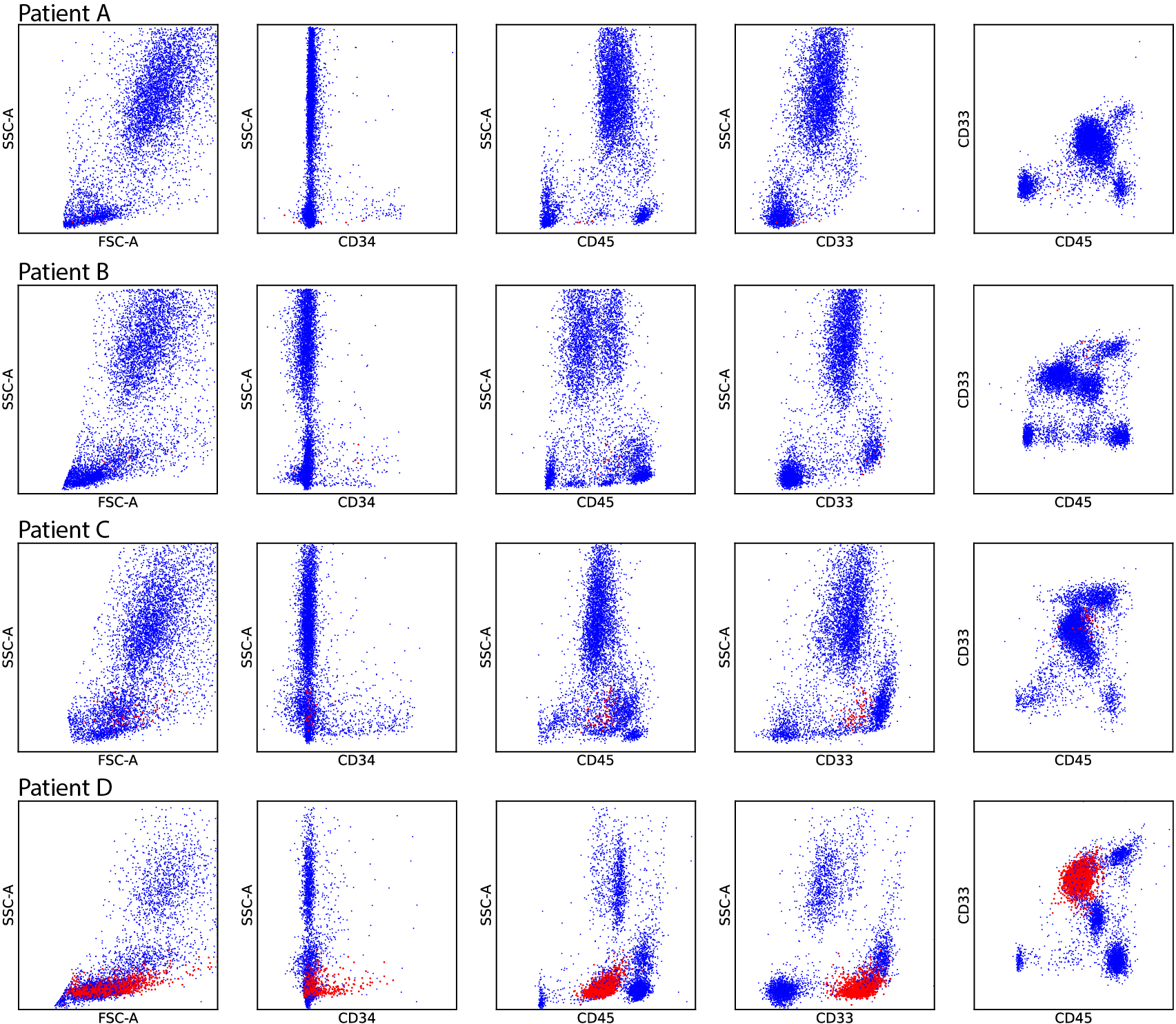
Figure 3: This figure shows 2D projections of samples from the AML-MRD dataset on different combination of features. Each dot corresponds to one event i.e. the feature measurement vector of one cell. Cancer cells are marked in red, healthy in blue. Each row corresponds to a different patient.

Appendix B Features

All four datasets combined have 35 features in total including forward- (FSC) and side-scatter (SSC) of the laser light. FSC and SSC measure physical properties of the cell, like size and granularity. The rest of the features correspond to fluorescent-labeled surface markers, of which the concentration is measured. Different cell types bind to different surface markers and hence, those markers enable to separate and analyse cell-types. A detailed listing of what features in how many samples are present for each dataset is given in Tab. 5. ”CD” stands for cluster of differentiation. ”A”, ”H” an ”W” stands for area, hight and width, respectivley in the FSC and SSC. We just speak of FSC and SSC and do not necessarily differentiate between area, hight and width, since those are highly correlated. TIME indicates when the feature vector was acquired throughout the acquisition process of one sample and hence is not a strong discriminative feature. In total we can see that the AML-MRD and ALL-MRD datasets have the least in common with only 2 discriminative features excluding FSC and SSC throughout all samples, CD45 and CD34.

Table 5: List of features (markers) present in the datasets and their number of occurrences per dataset.

Feature	AML-MRD	CONTROL	DIA	ALL-MRD
FSC-A	71	308	110	338
FSC-H	66	131	58	0
FSC-W	71	253	99	338
SSC-A	71	308	110	338
SSC-W	67	185	52	1
CD38	32	164	52	338
CD371	32	163	52	0
CD34	71	308	110	338
CD117	71	308	110	0
CD33	71	308	110	0
CD71	5	6	28	0
CD123	33	165	53	0
CD45RA	32	164	52	0
HLA-DR	71	308	26	0
CD45	71	308	110	338
TIME	71	308	110	338
CD99	34	180	63	0
CD10	2	0	12	338
CD133	3	0	8	0
CD15	39	161	57	0
CD11A	18	11	13	0
CD7CD56	5	1	3	0
CD14	39	161	57	0
CD11B	39	161	57	0
CD13	14	132	35	0
NG2	3	2	4	0
CD56	12	0	0	0
CD7	15	15	11	0
CD312	5	0	1	0
CD16	2	0	14	0
CD48	1	0	2	0
CD58	0	0	0	138
CD19	0	3	3	338
CD20	0	0	0	338
SY41	0	0	0	338

Appendix C Patient Cross-Validation

The number of samples used for training, validation and testing are given in Tab. 6. Each patient determines one split. After precision $p$, recall $r$ and $F_{1}$-score have been determined for each sample in each test split, metrics are averaged over all samples to get the final results that are reported.

Table 6: The sample of the AML-MRD dataset are divided into training-, evaluation-, and test-set. Each patient’s samples exclusively form the test set, as indicated by the rightmost column specifying the sample count for each patient. The rest of the samples from different patients are allocated to the training and evaluation sets with a proportion of approximately $0.8$ and $0.2$, respectively.

Patient	Train	Eval	Test
A	56	14	1
B	51	15	5
C	47	14	10
D	54	13	4
E	53	13	5
F	49	11	11
G	42	11	18
H	56	13	2
I	54	15	2
J	51	11	9
K	56	13	2
L	54	15	2

Appendix D FATE-Decoder

Our Decoder proposed for the MAE experiments can be divided into a set-decoder and a feature-decoder part as described in the main text. Fig. 4 shows a detailed illustration of the two parts of the decoder.

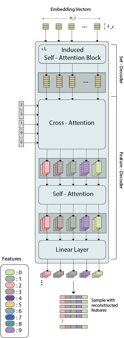
Figure 4: This figure illustrates the architecture of the decoder proposed for the MAE experiments. Input are the embedding vectors, which are put into context to each other with ISAB layers. It follows cross attention with the feature encodings of the features that should be reconstructed. Finally, the learnt vectors each corresponding to one feature value are attended to each other and mapped to its final reconstructed scalar feature value.

Appendix E Induced Self-Attention Block

We use the ISAB layers as proposed in [17]. Fig. 5 shows an illustration of the detailed architecture, where $n$ denotes the number of input set elements and $m$ the number of learnt queries i.e. induced points.

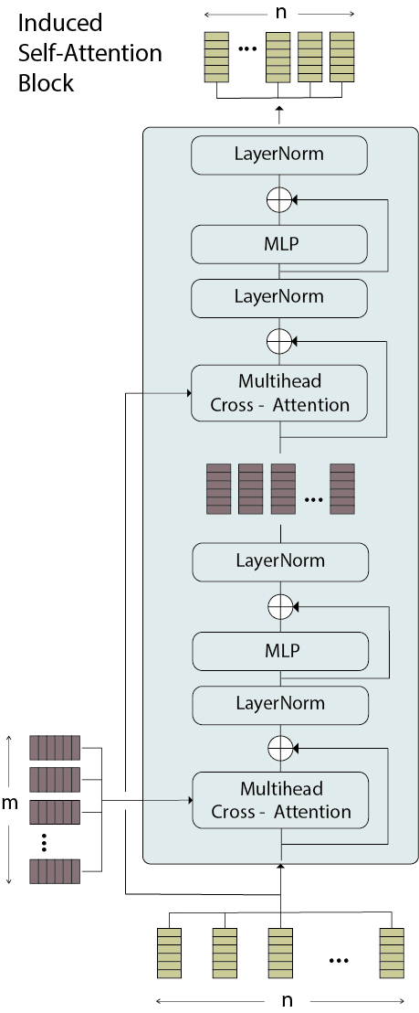
Figure 5: Illustration of the ISAB layer with an input set of $n$ elements and $m$ induced points [17]. Plus sign indicates additive skip connections.

Appendix F General Embedding of the FATE-MAE

Fig. 6 and Fig. 7 visualize the embedding of two different samples generated with the pretrained FATE-MAE with the CONTROL, DIA and ALL-MRD dataset with a masking ratio of $0.25\%$. We visualize healthy (blue) versus cancerous (red) cells (row 1 and 4) as well as clustering of cell populations (row 2 and 3). The figures show that the learnt embedding forms meaningful clusters of cells with respect to clusters of the original feature space.

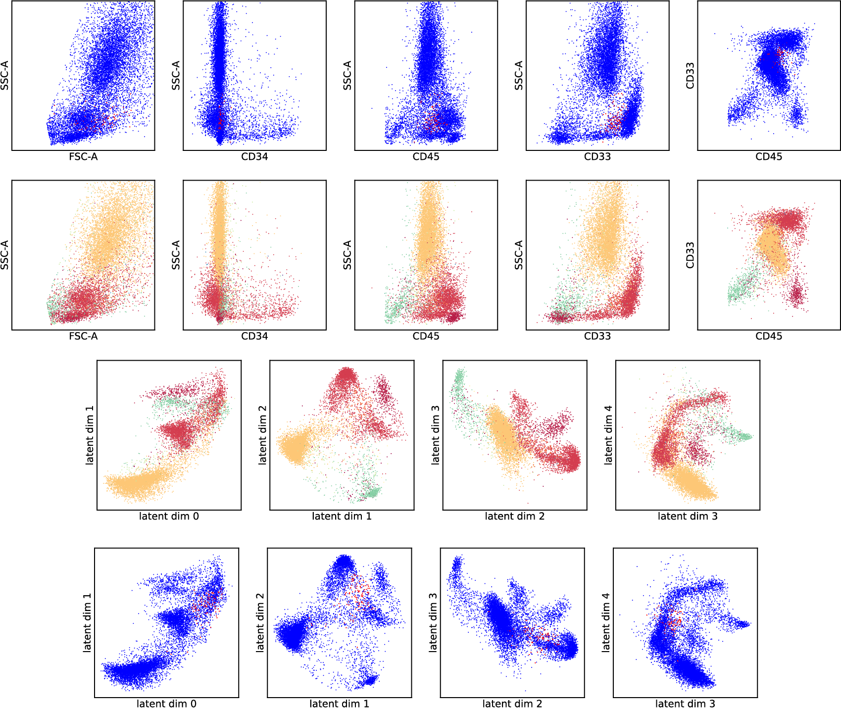
Figure 6: Visualization of a sample of Patient C from the AML-MRD dataset in its original feature space (row 1-2) and in the learnt general embedding space (row 3-4). Blue denotes healthy cells, red cancerous cells. The colours in row 2 and 3 indicate clusters of cell populations.

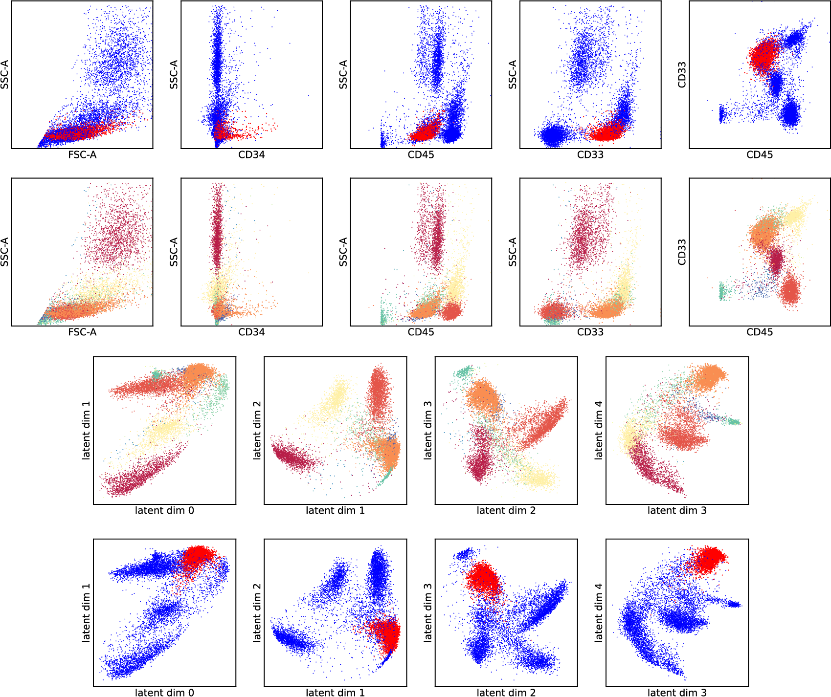
Figure 7: Visualization of a sample of Patient D from the AML-MRD dataset in its original feature space (row 1 -2) and in the learnt general embedding space (row 3-4). Blue denotes healthy cells, red cancerous cells. The colours in row 2 and 3 indicate clusters of cell populations.

References

- [1] Tamim Abdelaal, Thomas Höllt, Vincent van Unen, Boudewijn PF Lelieveldt, Frits Koning, Marcel JT Reinders, and Ahmed Mahfouz. Cytofmerge: integrating mass cytometry data across multiple panels. Bioinformatics, 35(20):4063–4071, 2019.
- [2] Tamim Abdelaal, Vincent van Unen, Thomas Höllt, Frits Koning, Marcel J.T. Reinders, and Ahmed Mahfouz. Predicting cell populations in single cell mass cytometry data. Cytometry Part A, 95(7):769–781, 2019.
- [3] Eirini Arvaniti and Manfred Claassen. Sensitive detection of rare disease-associated cell subsets via representation learning. Nature Communications, 8(14825):2041–1723, 2017.
- [4] Alan Baade, Puyuan Peng, and David Harwath. Mae-ast: Masked autoencoding audio spectrogram transformer. arXiv preprint arXiv:2203.16691, 2022.
- [5] Alexei Baevski, Wei-Ning Hsu, Qiantong Xu, Arun Babu, Jiatao Gu, and Michael Auli. Data2vec: A general framework for self-supervised learning in speech, vision and language. In International Conference on Machine Learning, pages 1298–1312. PMLR, 2022.
- [6] D Dalbokova, M Krzyzanowski, and S Lloyd. Children’s health and the environment in europe: a baseline assessment. World Health Organization. Regional Office for Europe, 2007.
- [7] Jacob Devlin, Ming-Wei Chang, Kenton Lee, and Kristina Toutanova. Bert: Pre-training of deep bidirectional transformers for language understanding. arXiv preprint arXiv:1810.04805, 2018.
- [8] Alexey Dosovitskiy, Lucas Beyer, Alexander Kolesnikov, Dirk Weissenborn, Xiaohua Zhai, Thomas Unterthiner, Mostafa Dehghani, Matthias Minderer, Georg Heigold, Sylvain Gelly, et al. An image is worth 16x16 words: Transformers for image recognition at scale. arXiv preprint arXiv:2010.11929, 2020.
- [9] Christoph Feichtenhofer, Yanghao Li, Kaiming He, et al. Masked autoencoders as spatiotemporal learners. Advances in neural information processing systems, 35:35946–35958, 2022.
- [10] Ritwik Giri, Fangzhou Cheng, Karim Helwani, Srikanth V. Tenneti, Umut Isik, and Arvindh Krishnaswamy. Group masked autoencoder based density estimator for audio anomaly detection. In Detection and Classification of Acoustic Scenes and Events Workshop 2020, 2020.
- [11] Yuan Gong, Andrew Rouditchenko, Alexander H Liu, David Harwath, Leonid Karlinsky, Hilde Kuehne, and James R Glass. Contrastive audio-visual masked autoencoder. In The Eleventh International Conference on Learning Representations, 2022.
- [12] Kaiming He, Xinlei Chen, Saining Xie, Yanghao Li, Piotr Dollár, and Ross Girshick. Masked autoencoders are scalable vision learners. In Proceedings of the IEEE/CVF conference on computer vision and pattern recognition, pages 16000–16009, 2022.
- [13] Zhenyu Hou, Yufei He, Yukuo Cen, Xiao Liu, Yuxiao Dong, Evgeny Kharlamov, and Jie Tang. Graphmae2: A decoding-enhanced masked self-supervised graph learner. In Proceedings of the ACM Web Conference 2023, pages 737–746, 2023.
- [14] Li Jiang, Zetong Yang, Shaoshuai Shi, Vladislav Golyanik, Dengxin Dai, and Bernt Schiele. Self-supervised pre-training with masked shape prediction for 3d scene understanding. In Proceedings of the IEEE/CVF Conference on Computer Vision and Pattern Recognition, pages 1168–1178, 2023.
- [15] Florian Kowarsch, Lisa Weijler, Matthias Wödlinger, Michael Reiter, Margarita Maurer-Granofszky, Angela Schumich, Elisa O. Sajaroff, Stefanie Groeneveld-Krentz, Jorge G. Rossi, Leonid Karawajew, Richard Ratei, and Michael N. Dworzak. Towards self-explainable transformers for cell classification in flow cytometry data. In Interpretability of Machine Intelligence in Medical Image Computing: 5th International Workshop, IMIMIC 2022, Held in Conjunction with MICCAI 2022, Singapore, Singapore, September 22, 2022, Proceedings, page 22–32, Berlin, Heidelberg, 2022. Springer-Verlag.
- [16] Georg Krispel, David Schinagl, Christian Fruhwirth-Reisinger, Horst Possegger, and Horst Bischof. Maeli–masked autoencoder for large-scale lidar point clouds. arXiv preprint arXiv:2212.07207, 2022.
- [17] Juho Lee, Yoonho Lee, Jungtaek Kim, Adam Kosiorek, Seungjin Choi, and Yee Whye Teh. Set transformer: A framework for attention-based permutation-invariant neural networks. In International Conference on Machine Learning, pages 3744–3753. PMLR, 2019.
- [18] Adrien Leite Pereira, Olivier Lambotte, Roger Le Grand, Antonio Cosma, and Nicolas Tchitchek. Cytobackbone: an algorithm for merging of phenotypic information from different cytometric profiles. Bioinformatics, 35(20):4187–4189, 2019.
- [19] Roxane Licandro, Thomas Schlegl, Michael Reiter, Markus Diem, Michael Dworzak, Angela Schumich, Georg Langs, and Martin Kampel. Wgan latent space embeddings for blast identification in childhood acute myeloid leukaemia. In 2018 24th International Conference on Pattern Recognition (ICPR), pages 3868–3873. IEEE, 2018.
- [20] Xiang Lin, Tian Tian, Zhi Wei, and Hakon Hakonarson. Clustering of single-cell multi-omics data with a multimodal deep learning method. Nature communications, 13(1):7705, 2022.
- [21] Kushal Majmundar, Sachin Goyal, Praneeth Netrapalli, and Prateek Jain. Met: Masked encoding for tabular data. arXiv preprint arXiv:2206.08564, 2022.
- [22] TR Mocking, C Duetz, BJ van Kuijk, TM Westers, J Cloos, and C Bachas. Merging and imputation of flow cytometry data: a critical assessment. Cytometry Part A, 2023.
- [23] Wanmao Ni, Beili Hu, Cuiping Zheng, Yin Tong, Lei Wang, Qing-qing Li, Xiangmin Tong, and Yong Han. Automated analysis of acute myeloid leukemia minimal residual disease using a support vector machine. Oncotarget, 7(44):71915–71921, 2016.
- [24] Christina Bligaard Pedersen, Søren Helweg Dam, Mike Bogetofte Barnkob, Michael D Leipold, Noelia Purroy, Laura Z Rassenti, Thomas J Kipps, Jennifer Nguyen, James Arthur Lederer, Satyen Harish Gohil, et al. cycombine allows for robust integration of single-cell cytometry datasets within and across technologies. Nature communications, 13(1):1698, 2022.
- [25] Shangran Qiu, Matthew I Miller, Prajakta S Joshi, Joyce C Lee, Chonghua Xue, Yunruo Ni, Yuwei Wang, Ileana De Anda-Duran, Phillip H Hwang, Justin A Cramer, et al. Multimodal deep learning for alzheimer’s disease dementia assessment. Nature communications, 13(1):3404, 2022.
- [26] Alec Radford, Jong Wook Kim, Chris Hallacy, Aditya Ramesh, Gabriel Goh, Sandhini Agarwal, Girish Sastry, Amanda Askell, Pamela Mishkin, Jack Clark, et al. Learning transferable visual models from natural language supervision. In International conference on machine learning, pages 8748–8763. PMLR, 2021.
- [27] Aditya Ramesh, Mikhail Pavlov, Gabriel Goh, Scott Gray, Chelsea Voss, Alec Radford, Mark Chen, and Ilya Sutskever. Zero-shot text-to-image generation. In International Conference on Machine Learning, pages 8821–8831. PMLR, 2021.
- [28] Michael Reiter, Markus Diem, Angela Schumich, Margarita Maurer-Granofszky, Leonid Karawajew, Jorge G Rossi, Richard Ratei, Stefanie Groeneveld-Krentz, Elisa O Sajaroff, Susanne Suhendra, et al. Automated flow cytometric mrd assessment in childhood acute b-lymphoblastic leukemia using supervised machine learning. Cytometry Part A, 95(9):966–975, 2019.
- [29] Michael Reiter, Paolo Rota, Florian Kleber, Markus Diem, Stefanie Groeneveld-Krentz, and Michael Dworzak. Clustering of cell populations in flow cytometry data using a combination of gaussian mixtures. Pattern Recognition, 60:1029–1040, 2016.
- [30] Sören Richard Stahlschmidt, Benjamin Ulfenborg, and Jane Synnergren. Multimodal deep learning for biomedical data fusion: a review. Briefings in Bioinformatics, 23(2):bbab569, 2022.
- [31] Kaveri A Thakoor, Jiaang Yao, Darius Bordbar, Omar Moussa, Weijie Lin, Paul Sajda, and Royce WS Chen. A multimodal deep learning system to distinguish late stages of amd and to compare expert vs. ai ocular biomarkers. Scientific reports, 12(1):2585, 2022.
- [32] Ashish Vaswani, Noam Shazeer, Niki Parmar, Jakob Uszkoreit, Llion Jones, Aidan N Gomez, Łukasz Kaiser, and Illia Polosukhin. Attention is all you need. In Advances in neural information processing systems, pages 5998–6008, 2017.
- [33] Pascal Vincent, Hugo Larochelle, Yoshua Bengio, and Pierre-Antoine Manzagol. Extracting and composing robust features with denoising autoencoders. In Proceedings of the 25th international conference on Machine learning, pages 1096–1103, 2008.
- [34] Zihao Wang, Wei Liu, Qian He, Xinglong Wu, and Zili Yi. Clip-gen: Language-free training of a text-to-image generator with clip. arXiv preprint arXiv:2203.00386, 2022.
- [35] Matthias Wodlinger, Michael Reiter, Lisa Weijler, Margarita Maurer-Granofszky, Angela Schumich, Stefanie Groeneveld-Krentz, Richard Ratei, Leonid Karawajew, Elisa Sajaroff, Jorge Rossi, and Michael N. Dworzak. Automated identification of cell populations in flow cytometry data with transformers. Computers in Biology and Medicine, page 105314, 2022.
- [36] Sanghyun Woo, Shoubhik Debnath, Ronghang Hu, Xinlei Chen, Zhuang Liu, In So Kweon, and Saining Xie. Convnext v2: Co-designing and scaling convnets with masked autoencoders. In Proceedings of the IEEE/CVF Conference on Computer Vision and Pattern Recognition, pages 16133–16142, 2023.
- [37] Jiale Xu, Xintao Wang, Weihao Cheng, Yan-Pei Cao, Ying Shan, Xiaohu Qie, and Shenghua Gao. Dream3d: Zero-shot text-to-3d synthesis using 3d shape prior and text-to-image diffusion models. In Proceedings of the IEEE/CVF Conference on Computer Vision and Pattern Recognition, pages 20908–20918, 2023.
- [38] Renrui Zhang, Ziyu Guo, Peng Gao, Rongyao Fang, Bin Zhao, Dong Wang, Yu Qiao, and Hongsheng Li. Point-m2ae: multi-scale masked autoencoders for hierarchical point cloud pre-training. Advances in neural information processing systems, 35:27061–27074, 2022.