CHEOPS observations of KELT-20 b/MASCARA-2 b: An aligned orbit and signs of variability from a reflective day side.

Abstract

Context. Occultations are windows of opportunity to indirectly peek into the dayside atmosphere of exoplanets. High-precision transit events provide information on the spin-orbit alignment of exoplanets around fast-rotating hosts.

Aims. We aim to precisely measure the planetary radius and geometric albedo of the ultra-hot Jupiter(UHJ) KELT-20 b along with the spin-orbit alignment of the system.

Methods. We obtained optical high-precision transits and occultations of KELT-20 b using CHEOPS observations in conjunction with simultaneous TESS observations. We interpreted the occultation measurements together with archival infrared observations to measure the planetary geometric albedo and dayside temperatures. We further used the host star’s gravity-darkened nature to measure the system’s obliquity.

Results. We present a time-averaged precise occultation depth of 82$\pm$6 ppm measured with seven CHEOPS visits and 131${}^{+8}_{-7}$ ppm from the analysis of all available TESS photometry. Using these measurements, we precisely constrain the geometric albedo of KELT-20 b to 0.26$\pm$0.04 and the brightness temperature of the dayside hemisphere to 2566${}^{+77}_{-80}$ K. Assuming Lambertian scattering law, we constrain the Bond albedo to $0.36^{+0.04}_{-0.05}$ along with a minimal heat transfer to the night side ($\epsilon=0.14^{+0.13}_{-0.10}$). Furthermore, using five transit observations we provide stricter constraints of $3.9\pm 1.1$ degrees on the sky-projected obliquity of the system.

Conclusions. The aligned orbit of KELT-20 b is in contrast to previous CHEOPS studies that have found strongly inclined orbits for planets orbiting other A-type stars. The comparably high planetary geometric albedo of KELT-20 b  corroborates a known trend of strongly irradiated planets being more reflective. Finally, we tentatively detect signs of temporal variability in the occultation depths, which might indicate variable cloud cover advecting onto the planetary day side.

1 Introduction

Occultations (or secondary eclipses) are windows of opportunity to study exoplanetary atmospheres. An occultation depth is a measure of the planet’s brightness that manifests in a subtle decrease in the observed flux as it goes behind (is occulted by) the star. This brightness consists of two components: the stellar light reflected off the planet’s visible hemisphere and its thermal emission. For ultra-hot Jupiters (UHJs) observed in optical passbands, the contribution of the planet’s thermal emission to its brightness is comparable to the predominant reflection contribution. Consequently, the measured occultation depth is a degenerate combination of the two, making it difficult to disentangle their respective contributions. This degeneracy can be broken with additional information, such as occultation depth measurements in different passbands.

KELT-20 b (Lund et al. 2017) or MASCARA-2b (Talens et al. 2018) was first reported simultaneously in the two discovery papers from the KELT (Pepper et al. 2018) and MASCARA (Snellen et al. 2012) transit surveys, respectively. Both surveys use dedicated ground-based telescopes for exoplanet discoveries, particularly the brightest transiting exoplanet systems. KELT-20 b is a transiting UHJ that orbits one of the hottest ($T_{\rm eff}$ $\sim$9000 K) fast-rotating ($v\sin i_{\star}$ $\sim$116 km s^-1) stars in a $\sim$3.5 day orbit. This leads to an equilibrium temperature of $T_{\rm eq}$ $\sim$2300 K (see Table 1 for details on stellar parameters).

By virtue of many follow-up observations in the form of high-resolution transmission spectroscopy, the atmosphere of KELT-20 b has been well characterised with the detection of the following species: Na, H$\alpha$, Mg, Fe, Fe I, Fe II, Ca⁺, Cr II, Si (Casasayas-Barris et al. 2018, 2020; Stangret et al. 2020; Hoeijmakers et al. 2020a; Nugroho et al. 2020; Cont et al. 2022). The day side of KELT-20 b is hotter than the theoretical equilibrium temperature because of the intense far-ultraviolet (FUV) and ultraviolet (UV) radiation received from its host A2 star, which heats up the upper layers of the atmosphere, leading to the expansion and abrasion of species between different layers Fu et al. (2022). The FUV/UV radiation also facilitates the presence of a strong thermal inversion in the underlying layers, which is evident from the additional detection of neutral and atomic iron in the emission lines (Yan et al. 2022; Borsa et al. 2022). Consequently, the atmosphere is inflated enough to show strong absorption in the transmission spectrum, and the host star is sufficiently hot to strengthen the atomic/molecular spectral signatures in the emission spectrum leading to a plethora of species discoveries, including the likes of CO and H2O (Fu et al. 2022). Furthermore, Rainer et al. (2021) observed both the classical and the atmospheric Rossiter–McLaughlin (RM) effect by studying the Fe I feature in transmission. This detection of the blue-shift in the atmospheric signal during the transit along with the well-resolved double peak of the Fe I spectral feature in the emission spectrum (Nugroho et al. 2020) provides possible indications of atmospheric variability.

Table 1: Stellar parameters from SWEET-CAT catalogue used in this work.

Parameter	Symbol	Units	Value	Source
			MASCARA-2
Aliases			HD 185603	Simbad
			TIC 69679391 / TOI-1151
Spectral Type			A2V	Talens et al. (2018)
Effective temperature	$T_{\rm eff}$	K	$8980^{+30}_{-130}$	Lund et al. (2017)
Surface gravity	$\log g$	$\log{\mathrm{cm/s^{2}}}$	$4.31\pm 0.02$	Lund et al. (2017)
Density	$\rho_{\star}$	$\mathrm{g/cm^{3}}$	$0.641^{+0.035}_{-0.033}$	Lund et al. (2017)
Metallicity	[Fe/H]	—	$-0.02\pm 0.07$	Lund et al. (2017)
Projected rotational velocity	$v\sin i_{\star}$	km/s	$116.23\pm 1.25$	Rainer et al. (2021)
Stellar rotation period	$P_{\mathrm{rot}}$	d	0.696$\pm$0.027	Lund et al. (2017)
RV semi amplitude		m/s	${<322.51}$	Casasayas-Barris et al. (2019)
Stellar mass	$\rm M_{\star}$	$\rm M_{\sun}$	$1.89_{-0.05}^{+0.06}$	Talens et al. (2018)
Stellar radius	$\rm R_{\star}$	$\rm R_{\sun}$	$1.60\pm 0.06$	Talens et al. (2018)

The study of exoplanet atmospheres, particularly hot Jupiters, has already benefited from the high-precision occultation measurements with CHEOPS (Lendl et al. 2020; Hooton et al. 2022; Deline et al. 2022; Brandeker et al. 2022; Scandariato et al. 2022; Jones et al. 2022; Parviainen et al. 2022; Krenn et al. 2023). One of the new frontiers in exoplanetology is the detection of atmospheric variability measured as variations in the occultation depth and the phase curve’s peak offset over time. Previous studies of atmospheric variability with Spitzer in the canonical hot Jupiters HD 209458b and HD 189733b did not show any variability with robust statistical significance (Kilpatrick et al. 2020). The first claim of atmospheric variability was announced for HAT-P-7 b (Armstrong et al. 2016) using the Kepler phase curves and later in Kepler-76 b (Jackson et al. 2019). Both of these studies found strong variations in the longitude of the brightest point in the planets’ atmospheres, although the former was recently attributed to photometric variability due to super-granulation in the host star (Lally & Vanderburg 2022). With increasing photometric precision and multi-epoch observations, more reports of exoplanet variability become prevalent (Hooton et al. 2019; Wilson et al. 2021; Parviainen et al. 2022).

In this paper we present precise transit and occultation depths of KELT-20 b using the data from its observation with the CHaracterising ExOplanet Satellite (CHEOPS  Benz et al. 2021) and the Transiting Exoplanet Survey Satellite (TESS  Ricker et al. 2014). We present all the datasets in Sect. 2.1 together with the description of the data reduction. In Sect. 3 we describe the planetary light curve fitting algorithms used in this article. In Sect. 4 we present the results of our analysis, and discuss the outcomes in Sect. 5. Finally in Sect. 6 we draw our conclusions.

2 Observations and data reduction

2.1 CHEOPS observations

CHEOPS observed the KELT-20 system in the consecutive summers of 2021 and 2022. The first set of observations include four secondary eclipses and four primary transits of the planet KELT-20 b extended over a period of two months starting from June 25 to September 1, 2021, while the second includes three additional secondary eclipses and one more primary transit that were observed from July 2 to August 9, 2022 (8). Each visit was centred around either the secondary eclipse or the primary transit using the ephemerides from Lund et al. (2017), with the total observation time equal to three times the eclipse or transit duration. Consequently, each visit spanned an average of 10 to 11 hr where a time series was acquired with a cadence of 36 s. Due to interruptions from Earth occultations and crossings over the South Atlantic Anomaly (SAA) and to data flagging by the data reduction pipeline (DRP), the efficiency (i.e. the fraction of the visit time leading to scientifically valuable observations) was $\sim$67%. All the information about the individual observations, which were part of two different CHEOPS Guaranteed Time Observation (GTO) subprogrammes, is summarised in Table 2.

Table 2: Logbook of the CHEOPS observations of KELT-20. The top seven are the occultation observations while the bottom five are the transits.

File-key	Visit	Start time	Duration	N. frames	Efficiency	Rjct. pts.
	ID	[UTC]	[hr]		[%]
CH_PR100016_TG014101_V0200	1520194	2021-06-25 12:43:51	10.98	747	69.6	78
CH_PR100016_TG014102_V0200	1533914	2021-07-12 22:48:52	11.22	695	64.2	70
CH_PR100016_TG014103_V0200	1543424	2021-07-29 07:02:51	10.96	747	69.7	69
CH_PR100016_TG014104_V0200	1566969	2021-08-12 04:01:51	10.98	772	71.5	80
CH_PR100016_TG014105_V0200	1840687	2022-07-02 05:59:52	11.22	682	62.8	78
CH_PR100016_TG014106_V0200	1850916	2022-07-16 03:59:51	10.87	705	66.6	74
CH_PR100016_TG014107_V0200	1878526	2022-08-09 11:37:51	10.68	684	66.2	71
CH_PR110047_TG000401_V0200	1532996	2021-07-11 04:05:52	11.0	664	62.8	64
CH_PR110047_TG000402_V0200	1532997	2021-07-14 16:57:51	9.8	621	64.8	53
CH_PR110047_TG001001_V0200	1564166	2021-08-11 10:50:51	9.31	612	67.7	63
CH_PR110047_TG001002_V0200	1580776	2021-09-01 09:39:51	9.28	609	67.1	72
CH_PR100020_TG000801_V0200	1869414	2022-07-28 08:48:49	10.83	716	64.9	79

2.2 Data reduction pipeline

Each CHEOPS observation was reduced by version 13.1.0 of the CHEOPS Data reduction pipeline Hoyer et al. (DRP, 2020). The processing summary of the pipeline includes standard calibration steps such as bias, gain, non-linearity, dark-current, and flat fielding, and the correction for the environmental affects such as cosmic rays, smearing trails from nearby stars, and the sky background. Following the corrections, the photometric extraction was performed over four aperture sizes, three predefined and one optimised aperture size corresponding to the best signal-to-noise ratio (S/N). The default S/N (25 pixels) is comparable to that of the optimal aperture size that varies between 15 and 19 pixels for different observations. The dispersion of the photometric light curve is lower with the former, and therefore we used the photometric extraction done with the default aperture radius instead of the optimal one. The field of view (FoV) of KELT-20 is populated with a few nearby background stars. The DRP estimated the contamination of these nearby objects by simulating the CHEOPS FoV based on the Gaia DR2 star catalogue (Gaia Collaboration et al. 2021) and a template of the extended CHEOPS point spread function (PSF). To further analyse the DRP data, we used the PyCHEOPS software package developed specifically for the analysis of CHEOPS light curves (Maxted et al. 2022).

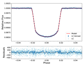
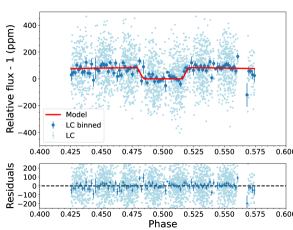
Figure 1: CHEOPS light curve. Left: Detrended and phase-folded planetary transits. The solid red line is the best-fit model, while the blue dots represent the phase-folded and binned photometry (Interval: 2.25 minutes for transit, 7.5 minutes for occultation). The residuals are shown in the bottom panel. Right: Same as in the left panel, but centred at the occultations.

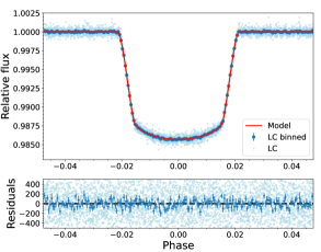
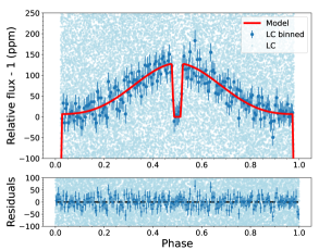
Figure 2: TESS light curve. Left: Detrended and phase-folded planetary transits from Sectors 14, 40, 41, and 54. The solid red line is the best-fit model, while the blue dots represent the phase-folded and binned photometry (Interval: 2.25 minutes for transit, 25 minutes for phase curve). The residuals are shown in the bottom panel. Right: Combined phase curve using photometry from all four sectors.

2.3 Detrending using point spread function

Due to the nature of the CHEOPS orbit, the presence of nearby background stars within the FoV can cause repeating flux variations on the timescales of the spacecraft’s orbital period. These variations are in correlation with the roll angle of the telescope. Therefore, to account for such systematic changes, we need to simultaneously use sinusoidal detrending vectors to the DRP light curve during model fitting. These features are already present in the PyCHEOPS package, and we used them in our DRP light curve analysis. Additionally, it has been observed that such flux variations lead to subtle modifications to the target PSF (e.g. Lendl et al. 2020; Bonfanti et al. 2021; Wilson et al. 2022). Upon closer inspection of our KELT-20 data, we found this characteristic systematic, and thus applied the PSF-SCALPELS algorithm (Wilson et al. 2022) to the DRP photometry. In brief, PSF-SCALPELS corrects flux modulations due to PSF shape changes by conducting a principal component analysis on the auto-correlation function of the photometric frames. This set of principal components traces variations in the PSF from the images, and is used in a linear noise model to detrend light curve fluxes. A more detailed explanation can be found in Wilson et al. (2022) with further examples of use shown in Hoyer et al. (2022), Parviainen et al. (2022), Hawthorn et al. (2023), and Ehrenreich et al. (2023).

While PSF-SCALPELS is a PSF-based correction to the DRP photometry, we also performed an independent photometric extraction using the PSF Imagette Photometric Extraction pipeline (PIPE) package Morris et al. (2021); Brandeker et al. (2022). We found that the dispersion in the reduced light curves are compatible with that of the other extraction techniques. They vary around a median absolute deviation (MAD) of 150 ppm at the raw cadence of 36 seconds. The light curves with PIPE extraction are free from roll angle variations and do not require additional detrending. Consequently, the error bars on the resultant fit parameters are smaller compared to those obtained via other techniques. We therefore chose to use the PIPE extracted photometry for further light curve analysis. Nevertheless, we show a comparative measurement of the occultation depths analysed using the three data extraction pipelines in Fig. 9. This exercise demonstrates the robustness of the extraction techniques, and further enhances confidence in the final outcome.

2.4 Outlier removal

Prior to the light curve analysis, we first filtered out the generic outliers flagged by PIPE that could have originated from cosmic ray encounters, centroid shifts far away from the median centroid, noisy bad pixels, or a poor PSF fit. The data points in the light curve corresponding to these images were masked out from further analysis. In addition, we also discarded data points where the flux is far above or below the median flux by setting a limit of five times the MAD value.

During each CHEOPS orbit, the observations are interrupted by Earth occultations. In proximity to the occultations, the background flux is drastically pushed up by scattered light from the Earth, leading to increased scatter in the light curve as it closes to the Earth’s occultation. We decided to remove the data points whose corresponding background flux exceeds the median value by more than three times the median absolute deviation. We proceeded with the leftover good data points and fitted them with the planetary model discussed in the next section.

2.5 TESS observations

TESS observed the KELT-20 system in Sector 14 (July 18 to August 14, 2019), Sectors 40–41 (June 25 to August 20, 2021), and in Sector 54 (July 9 to August 5, 2022). We downloaded the 2 min cadence pre-searched data conditioning single aperture photometry (PDC-SAP) light curves (Jenkins et al. 2016) using the lightkurve package (Lightkurve Collaboration et al. 2018). The light curves were corrected for instrumental systematics following Smith et al. (2012); Stumpe et al. (2012, 2014). We also experimented with single aperture photometry (SAP) light curves. We found conflicting results between the PDC-SAP and the SAP detrended light curve analysis; the results of the former are consistent with the CHEOPS results, and therefore we present only the PDC-SAP light curve analysis.

3 Light curve analysis

3.1 Planetary model

Our light curve model $F(\phi)$ is defined as the sum of the contributions from several independent submodels related to planetary and stellar flux variations. These include a primary transit $F_{\rm tr}(\phi)$ and an occultation $F_{\rm occ}(\phi)$ model with a flat out-of-eclipse baseline; a phase variation $F_{\rm day}(\phi)$ model corresponding to the flux from the planetary day side and a similar nightside phase variation term $F_{\rm nt}(\phi)$, an ellipsoidal variation (Morris 1985; Mislis et al. 2012) term $F_{\rm EV}(\phi)$, and a Doppler boosting (Loeb & Gaudi 2003; Barbier & López 2021) term $F_{\rm DB}(\phi)$ corresponding to the changes in stellar flux. For KELT-20 b the combined amplitude of $F_{\rm EV}(\phi)$ and $F_{\rm DB}(\phi)$ are of the order of unity ($\sim$2 ppm), which stands below the measured uncertainties, while the phase amplitude corresponding to the planetary brightness is of the order of tens of ppm, and therefore we excluded the former from our phase curve modelling. The final model constitutes the following:

$$F(\phi)=f_{0}+F_{\mathrm{tr}}(\phi)+F_{\mathrm{occ}}(\phi)+F_{\mathrm{day}}(\phi)+F_{\mathrm{night}}(\phi),$$ (1)

where $\phi$ is the planet’s orbital phase and $f_{0}$ is an arbitrary additive offset to align the light curve such that the base of the eclipse is at a relative flux value equal to one. The complete mathematical description can be found in Esteves et al. (2013) and references therein. Our model assumes a tidally locked circular orbit for KELT-20 b following Wong et al. (2021). We used the Mandel & Agol (2002) transit model of a circular disc passing over a spherical stellar disc with the following parametrisation:

• mid-transit epoch $T_{0}$;

• orbital frequency $\nu_{\mathrm{orb}}$ (inverse of the orbital period $P_{\mathrm{orb}}$);

• stellar density $\rho_{\star}$;

• planet to star radius ratio $R_{p}/R_{\star}$;

• impact parameter $b$;

• the re-parametrised quadratic limb darkening coefficients $q_{1}$ and $q_{2}$ (Kipping 2013).

The occultation model follows a similar description, with the difference that the smaller disc is passing behind the larger one and without any limb darkening law. This description was applied in previous works (Singh et al. 2022; Scandariato et al. 2022). The planetary brightness at superior conjunction is parametrised by an occultation depth $\delta_{\mathrm{occ}}$. The phase variation term $F_{\mathrm{day}}(\phi)$ models the changing planetary flux emanating from the day side during its orbital motion, which is parametrised by an amplitude term $A_{\mathrm{day}}$ and a brightness variation term defined by the reflected light phase function (Esteves et al. 2015; Singh et al. 2022). The dayside phase variation is a consequence of Lambertian radiation from both reflection and thermal emission. A dayside phase offset $\Delta\phi$ is included to account for the asymmetry in the phase variation Scandariato et al. (2022). We followed the convention where positive $\Delta\phi$ implies an eastward phase shift, while negative is for westward shift. We also incorporate a similar but inverted phase function for thermal emission from the night side, which is parametrised by $A_{\mathrm{night}}$. No phase offset term is included, and therefore it peaks at mid-transit, while the minima is at mid-eclipse. The minima of the dayside flux is at mid-transit, while the minima of the nightside flux is at mid-occultation. The eclipse depth from these three parameters is obtained by the following equation:

$$\delta_{\mathrm{occ}}=F_{\mathrm{day}}(\phi=0.5)+A_{\mathrm{night}}.$$ (2)

We followed this description along with the transit parameters while fitting the full phase curve. Phase curves are only available for the TESS light curves; the CHEOPS observations do not have phase information, and therefore we followed a simpler description with $F_{\mathrm{night}}=0$. To take into account that white noise is not included in the formal photometric uncertainties, we added an independent jitter term to our model.

We fitted the data with the combined model and searched for the simultaneous convergence of the free parameters by maximising the log-likelihood function in the parameter space. We sampled the posterior probability distribution of the free model parameters in a Bayesian MCMC framework using the emcee package version 3.0.2 (Foreman-Mackey et al. 2013). We followed the base line criterion of convergence following the methods described in Goodman & Weare (2010). Under the situations where we had to choose among a set of different models, we followed the Akaike information criterion (AIC, Burnham & Anderson (1998)) because of its robustness in information extraction without strongly penalising any additional model parameters. Given the complexity and demand of resources, we performed all our model fitting on the AMONRA computing infrastructure (Bertocco et al. 2020; Taffoni et al. 2020).

3.2 Transit model with gravity darkening

KELT-20 is an A2V star with a $v\sin i_{\star}$ of 116 km/s and a radius of 1.6 $R_{\sun}$ resulting in a rotation period of $\sim$1 day and is therefore categorised as a fast-rotator. The centrifugal force at the surface of fast-rotating stars is non-negligible compared to the stellar gravitational force. Consequently, the stellar gravity is highest at the poles and lowest at the equators, creating an oblate star. According to the von Zeipel theorem, the radiative flux at a given latitude of a fast-rotating star is proportional to the local effective gravity (von Zeipel 1924). The flux radiated at equatorial stellar latitudes is significantly lower compared to the poles. This effect is referred to as gravity darkening (GD). During a transit, when a planet passes over and hides the varying brightness of the stellar surface, it generates an asymmetric transit curve, especially when the orbit is misaligned. The greater the projected orbital obliquity $\lambda_{p}$, the larger the asymmetry (Lendl et al. 2020; Deline et al. 2022; Hooton et al. 2022). In addition, high-precision transit analysis is the preferred technique in measuring the true obliquity ($\Psi$) of a planetary system. Using the stellar and orbital inclinations, it is computed by the following relation

$$\cos{\Psi}=\cos{i_{\star}}\cos{i_{\mathrm{p}}}+\sin{i_{\star}}\sin{i_{\mathrm{p}}}\cos{\lambda}.$$ (3)

We model the GD transits of KELT-20 using the Transit Light Curve Modeler (TLCM; Csizmadia 2020, Csizmadia et al. 2023), which was used to model GD in the WASP-189 (Lendl et al. 2020), MASCARA-1 (Hooton et al. 2022), and WASP-33 (Kálmán et al. 2022) systems. The fitted GD parameters in TLCM are the inclination of the stellar rotation axis, $i_{\star}$, and the longitude of the node of the stellar rotation axis, $\Omega_{\star}$, which is directly related to the sky-projected spin-orbit obliquity, $\lambda$, via $\cos\lambda=\pm\cos(\Omega_{\mathrm{p}}-\Omega_{\star})$, where $\Omega_{\mathrm{p}}$ is the planetary rotational axis and is set to $90^{\circ}$. The GD exponent, $\beta$, is typically set to its theoretically expected value of 0.25 following von Zeipel’s law (von Zeipel 1924). Along with the GD parameters, the model describes the transits using the following fitted parameters: the scaled orbital semi-major axis, $a/R_{\star}$; the planet-to-star radius ratio, $R_{\mathrm{p}}/R_{\star}$; the transit impact parameter, $b$; the epoch of mid-transit; the orbital period, $P$; and the limb-darkening parameters, $u_{+}$ and $u_{-}$, related to the quadratic limb-darkening parameters, $u_{1}$ and $u_{2}$, via $u_{+}=u_{1}+u_{2}$ and $u_{-}=u_{1}-u_{2}$. Two additional parameters, $\sigma_{\mathrm{w}}$ and $\sigma_{\mathrm{r}}$, describe respectively the levels of white and red (correlated) noise present in the light curves, determined using the wavelet formulation of Carter & Winn (2009).

4 Results

In this section we present the outcomes of several of our analyses that include seven occultation and five transit observations of KELT-20 b with CHEOPS spanning over more than a year. Additionally, we also analysed the four TESS sectors of observations of KELT-20 that spanned over three years. We first present the results of the CHEOPS transit analysis with and without GD. We then present the results of only the occultation fits of both the telescopes followed by the results of the TESS phase curves.

Table 3: Best-fit model and derived parameters of the transit, occultation, and phase curve fit. G.D. represents gravity-darkening fit.

Parameter		Unit	CHEOPS	TESS
Transit
Stellar density	$\rho_{\star}$	$\mathrm{g/cm^{3}}$	$0.6501^{+0.0057}_{-0.0056}$	$0.6444^{+0.0053}_{-0.0052}$
Orbital frequency	$f$	$\mathrm{d^{-1}}$	$0.28784401\pm(33)$	$0.28784433\pm(23)$
Orbital Period	$P$	d	$3.4741039\pm(40)$	$3.47409999\pm(28)$
Orbital Period [G.D.]	-	d	$3.47410075\pm(56)$	$3.4741004\pm(04)$
Time of transit	$T_{c}$	BJD${}_{\rm TDB}-2457000$	2406.927174$\pm$(24)	1698.210775$\pm$(52)
Time of transit [G.D.]	-	-	$1312.5853\pm(02)$	$1312.5849\pm(01)$
Planet-star radius ratio	$R_{p}/R_{\star}$		$0.11572\pm 0.00018$	$0.11588\pm 0.00006$
Planet-star radius ratio [G.D.]	$R_{p}/R_{\mathrm{eq}}$		0.1131$\pm$0.0008	$0.1121\begin{subarray}{c}+0.0005\\ -0.0003\end{subarray}$
Impact parameter	$b$		$0.515\pm 0.005$	$0.523\pm 0.004$
Impact parameter [G.D.]	-		0.498$\pm$0.005	$0.510\pm 0.006$
Quadratic limb darkening	$q_{\mathrm{1}}$		$0.257\pm 0.018$	0.12$\pm$0.05
Quadratic limb darkening	$q_{\mathrm{2}}$		$0.322^{+0.036}_{-0.034}$	0.39$\pm$0.26
Quadratic limb darkening [G.D.]	$u_{a}+u_{b}$		0.516$\pm$0.021	$0.18\pm 0.03$
Quadratic limb darkening [G.D.]	$u_{a}-u_{b}$		$0.05\pm 0.10$	$0.39\pm 0.02$
Scaled semi-major axis	$a/R_{\star}$		$7.4579^{+0.0217}_{-0.016}$	$7.4359^{+0.0204}_{-0.0203}$
Scaled semi major axis [G.D.]	-	-	7.46$\pm$0.02	7.43$\pm$0.02
Stellar rotation axis	$i_{\star}$	deg	88.9${}^{+18.0}_{-19.8}$	$55\begin{subarray}{c}+9\\ -5\end{subarray}$
Nodal longitude	$\Omega_{\star}$	deg	86.12$\pm 1.10$	81$\pm$1
Orbital inclination	$i_{\rm p}$	deg	$86.03\pm 0.05$	$85.96\pm 0.04$
Orbital inclination [G.D.]	-	deg	$86.17\pm 0.04$	$86.064\pm 0.047$
Transit depth	$\delta_{\rm tr}$	%	$1.3391\pm 0.0042$	$1.3428\pm 0.0013$
Transit depth [G.D.]	$\left(\frac{R_{p}}{\sqrt{R_{\mathrm{pol}}R_{\mathrm{eq}}}}\right)^{2}$	%	1.3187 $\pm$ 0.019	1.296 $\pm$ 0.012
Sky-projected spin-orbit angle	$\lambda$	deg	$3.9\pm 1.1$	$9\pm 1$
Spin-orbit angle	$\Psi$	deg	$5.0\pm 11$	$32\pm 7$
Jitter	$\sigma_{\rm w}$	ppm	$123\pm 2$	$303\pm 4$
Red noise	$\sigma_{r}$	ppm	$1947\pm 107$	$7862\pm 284$
Occultation and phase-curve
Transit/Eclipse duration	T14 / t14	hr	$3.540\pm 0.003$	$3.537\pm 0.003$
Phase offset	$\Delta\phi$	deg	-	$-7^{+4}_{-7}$
Dayside Phase amplitude	$A_{\rm day}$	ppm	-	122.2$\pm$4.9*
Nightside Phase amplitude	$A_{\rm night}$	ppm	-	$8.6_{-5.8}^{+8.0}$
Occultation depth	$\delta_{\rm occ}$	ppm	$82.4\pm 5.6$	$131^{+8}_{-7}$
Brightness temperature (100% NIR)	$T_{\rm day}$	K	2759${}^{+200}_{-250}$	2555${}^{+200}_{-250}$
Geometric albedo (100% NIR)	$A_{\rm g}$		0.19$\pm$0.08	0.19$\pm$0.16
Lambertian grey-sky (CHEOPS – TESS)
Brightness temperature	$T_{\rm day}$	K	2566${}^{+77}_{-80}$
Geometric albedo	$A_{\rm g}$		$0.26\pm 0.04$
Dayside temperature	$T_{\mathrm{d}}$	K	$2618^{+35}_{-40}$
Nightside temperature	$T_{\mathrm{n}}$	K	$1266^{+259}_{-330}$
Bond albedo	$A_{\rm B}$		$0.36^{+0.04}_{-0.05}$
Heat re-circulation efficiency	$\epsilon$		$0.14^{+0.13}_{-0.10}$

4.1 Transits

4.1.1 Without gravity darkening

We fitted the five CHEOPS transit light curves individually following the model described in Sect. 3.1, where all the component models except for the transit ($F_{\mathrm{tr}}$) are set to zero. The best-fit parameters of the individual transit fits are reported in Table 6, while the same for the combined fit of all the transits are reported in Table 4. We present the best-fit transit model plotted over the phase folded photometry of all five transits in Fig. 1 (on the left). We also present the individual transit fits in Fig. 8. All the transits appear symmetrical with converging limb darkening coefficients, thereby implying an equatorial orbit for the hot Jupiter around the fast-rotator host. We compare the best-fit limb darkening coefficients ($q_{1}$ and $q_{2}$) reported in Table 4 with the theoretical estimates of $q_{1}=0.250\pm 0.001$ and $q_{2}=0.288\pm 0.001$, computed using the LDTk Python package Parviainen & Aigrain (2015), and found that their agreement is close to $1\leavevmode\nobreak\ \sigma$. This description is fairly consistent with that obtained with Doppler tomography (Hoeijmakers et al. 2020b). The transit parameters observed by CHEOPS agree with the measurements of the TESS photometry described later in Sect. 4.3. Figure 2 shows the best-fit plot of the TESS transits. The outcome of the TESS photometry agrees with previously reported literature values (Patel & Espinoza 2022; Wong et al. 2021).

4.1.2 With gravity darkening

With the aim of better constraining the obliquity of the KELT-20 system, we fitted the CHEOPS transit light curves with a GD model as described in Sect. 3.2. We placed a uniform prior $\mathcal{U}(80^{\circ},110^{\circ})$ on $\Omega_{\star}$, corresponding to $-10^{\circ}<\lambda<10^{\circ}$, based on Doppler tomography measurements of $\lambda$, which indicate that the KELT-20 system has an obliquity (sky-projected) close to zero Hoeijmakers et al. (2020a). Without this prior, the obliquity is poorly constrained by the transit photometry alone. We report our sky-projected ($\lambda$) and true obliquity ($\Psi$) values along with the other gravity darkening parameters in Table 4. The measured sky-projected obliquity in TESS differs from the same measured with CHEOPS. This could be due to some unaccounted for noise sources or degeneracy in the fitting the TESS  light curve. We present and compare our best-fit $\lambda$ along with the literature values in Section 5.4. The flattening parameter (f) is 0.03, which gives the planet’s polar-to-equatorial radius ratio $R_{\mathrm{pol}}/R_{\mathrm{eq}}$ at 0.97. Consequently, the planet-to-star radius ratio differs by more than 3$\sigma$ with and without GD model considerations. However, using the geometric mean as the stellar radius (i.e. $R_{\star}=\sqrt{R_{\mathrm{pol}}R_{\mathrm{eq}}}$ ) we reached an agreement between the two radius ratios.

We performed a similar analysis over the combined transits of the TESS photometry, and present it in Table 5. The fitting algorithm returns quite different outcomes compared to the CHEOPS transit fits. It returns a significantly inconsistent orientation of the KELT-20 system with a much lower radius ratio. This could be primarily attributed to the lower precision of the TESS light curves, and therefore a non-GD model best describes the transit light curve. Each sector’s individual TESS transits are shown in Figs. 10 and 11.

4.2 Occultations

CHEOPS observed a total of seven occultations of KELT-20 b, which we analysed individually and jointly. For these analyses we fitted the model as defined in Eq. 1, where the only free parameter is the occultation depth. We fixed the transit ephemerides following the TESS phase curve analysis described later in Sect. 4.3. We first fitted the data of only the occultation model along with a jitter term. Following which we found a correlation with the time, x and y pixel centroids, and the roll angle, and therefore we decided to include them as a co-detrending term. We obtain a clear detection of the occultation depth in all the visits with a precision of more than 3 $\sigma$ for the first and the last visit, and more than 5 $\sigma$ for the rest. The best-fit occultation depths of the individual visits are $46^{+13}_{-14}$, $77^{+14}_{-13}$, $105^{+13}_{-14}$, $102^{+13}_{-14}$, $71^{+15}_{-16}$, $125^{+18}_{-19}$, and $51\pm 15$ ppm. They are shown in Fig. 3 along with their posterior distributions in the side panel. The scatter of these measurements points towards a possible variability in the occultation depth of KELT-20b. The individual measurements are up to $2.8\,\sigma$ discrepant from their weighted mean, with the two most extreme measurements disagreeing by $3.4\,\sigma$. Conscious that the small sample size complicates a thorough statistical evaluation, we nevertheless attempted to quantify its significance. To do so, we created $10^{4}$ mock datasets assuming a constant occultation depth and measurements scattered around it following a Gaussian distribution with a width equal to the measurements’ uncertainties. From this distribution, we find a 0.3% probability (i.e. a p-value of 0.0033, or a $2.9\,\sigma$ significance) that measurements at least as discrepant as those observed are created randomly. While encouraging, this value hinges on the exact placement and uncertainty of each individual measurement, which hinges on the analysis approach (see Appendix 9), and the treatment of stellar and instrumental correlated noise. The leftover correlated noise in the best-fit residuals contributes $\sim 20\%$ to the uncertainty levels, the rest being the white noise. Considering this non-negligible red noise to some extent could contribute to the observed discrepancies in the occultation depth. On the other hand, it is noteworthy that the simultaneous TESS data (averaged in each sector) show a similar behaviour at lower significance, tentatively supporting the variability. Using all the visits, we obtain a mean occultation depth of 82$\pm$6 ppm, as shown by its posterior in the right plot of Fig. 1. We also present the individual occultation best-fits in the right panel of Fig. 8.

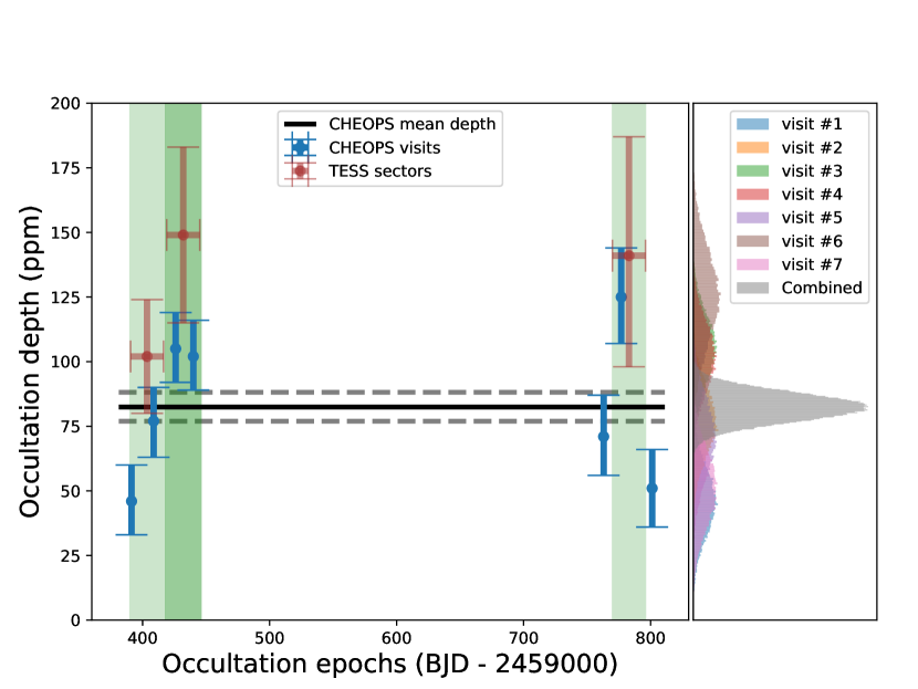
Figure 3: Best-fit occultation depths of individual CHEOPS visits (blue) along with their posteriors on the right. The horizontal solid and dashed lines represent the mean occultation depth of 82.4 $\pm$ 5.6 ppm. The panel on the right displays the best-fit posterior distribution. The green shaded regions indicate the span of the TESS Sectors 40, 41, and 54, while the brown points indicate the sector-wise occultation depths.

After finding the variability in the CHEOPS occultation depths, we looked for signs of variability in the TESS observations, which simultaneously observed the target during its Sector 40 and 41 orbits. The phase curve analysis from the second year of TESS has already been studied by Wong et al. (2021), and based on the four occultations in Sector 14, they report a depth of $111^{+35}_{-36}$ ppm. Fu et al. (2022) has analysed the occultation cuts from the three sectors observed at the time, and reports an average occultation depth of $139\pm 8$ ppm. Following the same approach, we eliminated the data points centred at the individual occultations that span over three times the duration. We then fitted the data with the occultation model along with a linear detrending term. Upon respective sector-wise analysis, we obtained occultation depths of $123\pm 36$, $105\pm 23$, $196\pm 32$, and $169\pm 29$ ppm. Consequently, we observe a 2 $\sigma$ difference in the measured depths between Sectors 40 and 41. This approach is convenient for obtaining an average measurement. However, a sector-wise comparison would need a complete planetary model with a better characterisation of the systematics present in the light curve.

4.3 TESS phase curves

We re-analysed the TESS light curves and fitted them with the complete model described in Section 3.1. We first fitted the model without any red noise correction term, and as a result we found strong short frequency trends in the residuals. To account for these low-frequency signals we simultaneously fitted the model with a Gaussian process (GP) model using a Matérn 3/2 kernel (Rasmussen & Williams 2006; Gibson et al. 2012). The Matérn 3/2 kernel defines the covariance between two observations at times $t_{i_{1}}$ and $t_{i_{2}}$ as

$$k(t_{i_{1}},t_{i_{2}})=h^{2}\left(1+\frac{\sqrt{3}|t_{i_{1}}-t_{i_{2}}|}{\lambda}\right)\exp\left(-\frac{\sqrt{3}|t_{i_{1}}-t_{i_{2}}|}{\lambda}\right)+j_{o}^{2}\delta_{i_{1},i_{2}},$$ (4)

where $h$ is the amplitude of the GP and $\lambda$ is its timescale. In order to take into account any additional white noise not included in the uncertainties, either instrumental or astrophysical, we added the diagonal terms $j_{o}^{2}\delta_{i_{1},i_{2}}$ to the Matérn 3/2 kernel, where $o$ denotes the TESS Sectors 14, 40, 41, and 54. Unfortunately, the precision in the TESS light curves is insufficient to provide precise constraints on the sector-wise phase offset and nightside flux. Phase offset and nightside flux convergence was reached only in the case of Sector 40 with values consistent with zero (i.e. $-11\pm 32$ degrees; see Fig. 13). Prior constraints on these parameters from the analysis of the Sector 14 phase curves were also consistent with zero (Wong et al. 2021). Hence, to reduce the dimensionality of the fit, we set these two parameters to zero. The parameters of the individual sector fits are presented in Table 7. The occultation depths measured with this approach are in agreement with the value measured in the previous section, although these depths lie towards the shallow end of the 1 $\sigma$ distribution obtained using the previous approach.

We fitted all four sectors, first independently and then simultaneously, with the same overall model parameters except the GP model hyper-parameters $h$ and $\lambda$, which are specific to correlated trends in individual sectors, although we kept a separate jitter term to account for the white noise. All the model parameters described in section 3.1 were kept free. The results of the best-fit parameters are presented in Table 4. The occultation depth is consistent with the previous analysis and literature values (Sect. 4.2). The best-fit model is shown in Figure 2 and the sector-wise independent model plots are shown in Fig. 12. We did not detect any significant nightside emission as $A_{\rm night}$ is consistent with zero within 1 $\sigma$. We report a 99.9% upper limit on $A_{\rm night}$ of 29 ppm, which corresponds to an upper limit to the nightside temperature at 2280 K. We also did not find any significant phase offsets as $\Delta\phi$ is consistent with zero.

5 Discussion

5.1 Atmospheric modelling

Given the bulk properties of KELT-20 b, we expect that thermal emission and stellar reflected signals both contribute to the planetary flux at the optical wavelengths probed by CHEOPS and TESS.

To provide a physical interpretation of the observed occultation depths, we modelled the planet’s emission spectrum using the open-source Pyrat Bay framework (Cubillos & Blecic 2021). This package employs parametric models of the planetary atmosphere (1D pressure profiles of the temperature, composition, and altitude), from which we then generate the thermal emission spectra. Using a Bayesian retrieval approach, the code constructs posterior distributions for the atmospheric parameters by fitting the emission models to observed occultation depth, using a differential-evolution MCMC (Cubillos et al. 2017). Since the Pyrat Bay code does not account for reflected light, we opted to constrain the thermal-emission models only by the infrared observations, which are largely dominated by the thermal component. We then computed the predicted thermal emission in the CHEOPS and TESS bands, and considered the reflected component as the difference between the observed and modelled fluxes.

We modelled the atmosphere from 100 to $10^{-9}$ bar, adopting a configuration similar to that of Fu et al. (2022). For the temperature profile we used the model of Guillot (2010), parametrised by the mean thermal opacity $\log_{10}(\kappa^{\prime})$, the ratio of visible and thermal opacities $\log_{10}(\gamma)$ to the irradiation temperature $T_{\rm irr}$. We assumed an atmospheric composition in chemical equilibrium, including the main species that dominate the chemistry for the molecules expected to be probed by the observations. These include H₂, He, H₂O, CH₄, CO, CO₂, N₂, HCN, NH₃, C₂H₂, C₂H₄, TiO, VO, TiO₂, VO₂, S₂, SH, SiO, H₂S, SO, and SO₂, as well as atomic and ionic species. To vary the atmospheric composition in the retrieval models, we used as parameters the abundance of metals [M/H], carbon [C/H], and oxygen [O/H], all relative to solar abundances in logarithmic scale. For these parameters we used a uniform prior ranging from 0.01 to 100 times solar (Table 4).

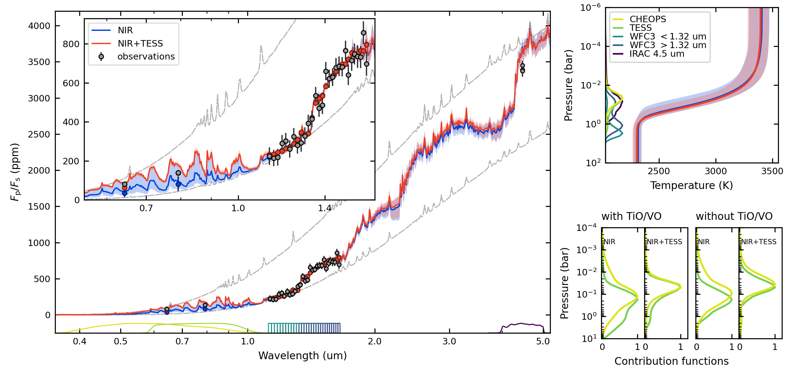
Figure 4: Left: KELT-20 b observed occultation depths (grey markers). The curve at the bottom shows the through-puts for each data point. The solid curves show the median of the retrieved model distributions when fitting the NIR HST and Spitzer occultations (blue) and the NIR+TESS occultations (red). The shaded areas (in corresponding colours) denote the span of the 68% central percentile of the distributions. The dashed grey curves show spectra for two black-body planetary model spectra at 2300 and 3200 K. Top right: Retrieved temperature profiles (same colour-coding as before). The curves at the left edge show the contribution functions for selected bands (see legend). Bottom right: Contribution functions integrated over the CHEOPS and TESS bands for the two cases shown in the left panel and for retrievals without TiO and VO opacity (same colour-coding as above). The band-integrated thermal flux in CHEOPS and TESS bands are ($36\pm 18$ ppm) and ($85\pm 38$ ppm), respectively (coloured markers).

We computed the emission spectra for each atmospheric model with a line-by-line radiative transfer routine sampling between 0.3 and 5.5 ${\umu\rm m}$ at a constant resolving power of $R=\lambda/\Delta\lambda=15\,000$. For the molecular opacities we used the data from HITEMP for CO, CO₂, and CH₄ (Rothman et al. 2010; Li et al. 2015; Hargreaves et al. 2020), and from ExoMol for H₂O, NH₃, HCN, TiO, and VO (Harris et al. 2006, 2008; Polyansky et al. 2018; Coles et al. 2019; Yurchenko 2015; McKemmish et al. 2016, 2019). Prior to the retrieval we pre-processed these large data files, first using the repack algorithm to extract the dominant line transitions (Cubillos 2017), and then tabulating the opacities over a fixed pressure, temperature, and wavelength grid. In addition, the model included Na and K resonant-line opacities (Burrows et al. 2000); collision-induced opacities for H₂–H₂ (Borysow et al. 2001; Borysow 2002); Rayleigh-scattering opacity for H, H₂, and He (Kurucz 1970); and a grey cloud deck model.

Figures 4 and 14 and Table 4 summarise our atmospheric retrieval results. To account for the unknown impact of reflected emission in the optical, we considered two retrieval scenarios: one fitting only the HST/WFC3 and Spitzer/IRAC near-infrared (NIR) occultation depths of Fu et al. (2022), and another that fits the NIR data and TESS occultation depth reported in this work.

The retrieval models fit the occultation data well, with the HST data dominating the thermal structure constraints. The higher emission seen in the longer wavelengths 1.3–1.6 $\umu\rm m$, where H₂O absorbs more strongly, drives the retrieval towards inverted temperature profiles. In terms of composition, both fits (with and without the TESS constraint) find a strong correlation between the carbon and oxygen abundances (Fig. 14). This results in broad carbon and oxygen posteriors, but a well-defined C/O ratio of less than one: C/O$=0.88^{+0.08}_{-0.23}$ (NIR retrieval) and C/O$=0.72^{+0.19}_{-0.22}$ (NIR+TESS retrieval). Including the TESS constraint has the largest impact on the [M/H] parameters, which accounts for the metallicity of all other species (most affected by the TESS constraint) and which narrows down to solar values from an otherwise largely unconstrained posterior. This occurs because the TESS band probes the absorption from species such as TiO, VO, Na, and K, which were previously unconstrained. The relatively high value of the TESS occultation depth drives the [M/H] constraint towards the upper values given the non-inverted thermal profile (higher emission from the hotter, upper layers of the atmosphere). Our results are generally consistent with those of Fu et al. (2022); both analyses find a clear thermally inverted temperature profile that quickly increases from $\sim$2300 K to $\sim$3400 K and C/O ratios close to the solar value (C/O${}_{\odot}=0.55$). In one additional test we explored cases excluding the absorption from TiO and VO, which are molecules that tend to condense out of planetary atmospheres (e.g., Hoeijmakers et al. 2020b). For these runs we found no significant variations in the retrieved properties (results consistent at the $1\sigma$ level).

In terms of thermal-light versus reflected-light flux, our NIR retrieval underestimates the TESS and CHEOPS occultation depths (Fig. 4), indicating that there must be a non-negligible reflected-light component. By including the TESS measurement in the fit, the model matches the TESS occultation depth, but still underestimates the CHEOPS occultation depth, again suggesting that there should be some fraction of reflected light in that band, although we note that this fit makes the implicit assumption that the TESS occultation depth is purely due to thermal emission. Therefore, these two scenarios model the planetary optical emission under two extreme cases: no prior assumption of reflected or thermal contribution (NIR retrieval) versus maximum thermal contribution (NIR+TESS retrieval). Our contribution functions indicate that TESS and Spitzer probe higher layers in the atmospheres than HST. In each scenario, the CHEOPS contribution functions coincide fairly well with that of TESS, suggesting that they probe a similar region in the atmosphere (Fig. 4).

Table 4: KELT-20 b Atmospheric retrieval. The reported values and uncertainties correspond to the median and 68% quantile of the marginal posterior distributions, respectively.

Parameter	Priors	Retrieved	Retrieved
		without TESS	with TESS
$\log_{10}(\kappa^{\prime})$	$\mathcal{U}(-8,-1)$	$-5.97^{+0.51}_{-0.21}$	$-6.02^{+0.37}_{-0.17}$
$\log_{10}(\gamma)$	$\mathcal{U}(-4,2)$	$0.67^{+0.04}_{-0.06}$	$0.67^{+0.04}_{-0.06}$
$T_{\rm irr}$ (K)	$\mathcal{U}(1000,3500)$	$2618^{+35}_{-40}$	$2610^{+35}_{-40}$
$[$M/H$]$	$\mathcal{U}(-2,2)$	$-0.79^{+0.75}_{-0.82}$	$-0.08^{+0.13}_{-0.10}$
$[$C/H$]$	$\mathcal{U}(-2,2)$	$-0.58^{+1.09}_{-0.63}$	$-0.74^{+0.94}_{-0.56}$
$[$O/H$]$	$\mathcal{U}(-2,2)$	$-0.73^{+1.03}_{-0.52}$	$-0.82^{+0.84}_{-0.40}$

5.2 Albedo

5.2.1 Geometric albedo and brightness temperature

A geometric albedo ($A_{g}(\lambda)$ or $A_{g,\lambda}$) is defined as the spherical albedo at full phase or phase angle $\alpha=0$ (superior conjunction, Seager 2010). It is defined as the ratio of the planet’s brightness to that of an idealised, flat, fully reflecting Lambertian disc with an identical cross-section. The brightness temperature ($T_{\mathrm{day}}(\lambda)$) of the planetary day side is the temperature of a black-body that emits the same amount of radiation within a specific passband. The T-P profile from Fig. 4 suggests that CHEOPS and TESS practically probe the same layer of the atmosphere that irradiates at similar temperatures, which are computed to be $2759^{+200}_{-250}$ and $2555^{+200}_{-250}$ K, respectively. Alternatively, following the HST/WFC3 + Spitzer/IRAC (NIR) model, we computed the band-integrated emission flux for both CHEOPS and TESS at 36$\pm$18 ppm and 85$\pm$38 ppm, respectively. As the resultant occultation depth is the sum of the two theoretical depths (i.e. $\delta_{\mathrm{occ}}=\delta_{\mathrm{ref}}+\delta_{\mathrm{thm}}$). Subtracting the emission flux from the observed depths listed in Table 4, we obtain the reflected flux and using Eq. 5 (Seager 2010), we obtain the band-integrated geometric albedos in the CHEOPS and TESS bands as $A_{g,{\mathrm{CHEOPS}}}=0.19\pm 0.08$ and $A_{g,{\mathrm{TESS}}}=0.19\pm 0.16$, respectively:

$$\delta_{\rm ref}=A_{g}\left(\frac{R_{p}}{a}\right)^{2}.$$ (5)

The geometric albedos in the two passbands are consistent with each other, as are the brightness temperatures from the T-P profile. Moreover, the retrieval model does not include scattering. In the absence of a detailed occultation spectrum at optical wavelengths, it is difficult to precisely predict the exact contribution of thermal emission or reflection to the planetary brightness. Therefore, to solve this degeneracy problem and to obtain stricter constraints on the dayside brightness temperature and the geometric albedo, we explored an alternate approach. Following the definition, we express the dayside emission in terms of the brightness temperature as Eq. 6 (Santerne et al. 2011; Singh et al. 2022):

$$\delta_{\rm thm}=\pi\left(\frac{R_{\rm p}}{R_{\star}}\right)^{2}\frac{\int_{\lambda}B_{\lambda}(T_{\mathrm{day}})\Omega_{\lambda}d\lambda}{\int_{\lambda}S_{\lambda}^{\rm CK}\Omega_{\lambda}d\lambda}\,.$$ (6)

Here $B_{\lambda}(T_{\mathrm{day}})$ is the Planck distribution for temperature $T_{day}$, $S_{\lambda}^{\rm CK}$ is the stellar Kurucz flux (Castelli & Kurucz 2003) for the nearest $T_{\rm eff}$, $\log{g}$, and [Fe/H]. The stellar flux and the planetary black-body flux is integrated over the telescope’s passband $\lambda$ with the corresponding response function $\Omega_{\lambda}$. We use the measured value of $\delta_{\mathrm{occ}}$ from observations together with Equations 5 and 6 to create a parametric relationship between the geometric albedo and the brightness temperature as

$$\frac{\alpha\delta_{\mathrm{occ}}^{\mathrm{CHEOPS}}-\delta_{\mathrm{occ}}^{\mathrm{TESS}}}{\left(\frac{R_{p}}{a}\right)^{2}}+\delta_{\mathrm{thm}}^{\mathrm{TESS}}-\alpha\delta_{\mathrm{thm}}^{\mathrm{CHEOPS}}=0,$$ (7)

where $\alpha$ denotes the ratio of the two geometric albedos (i.e. $A_{g}^{\mathrm{TESS}}/A_{g}^{\mathrm{CHEOPS}}$). Assuming identical band-integrated geometric albedos (or $\alpha=1$) and the same brightness temperatures in the two passbands, we can precisely constrain the two $A_{g}-T_{\mathrm{day}}$ pairs. Figure 5 shows the $A_{g}$ versus $T_{\mathrm{day}}$ relation for the occultation depths measured in the CHEOPS and TESS passbands. The brightness temperature is the independent parameter that varies from 1200 K to 3500 K. We do not expect negative values for the geometric albedo and are therefore truncated in the plot.

Being a wavelength-dependent property, $A_{g}$ might, in principle, vary between the TESS and CHEOPS bands (i.e. $\alpha\neq 1$); however, to constrain the $T_{\mathrm{day}}-A_{g}$ pair, we assume this variation to be below the precision of our data. This corresponds to one of two scenarios: (1) a grey-sky reflective atmosphere (i.e. a flat reflection spectrum) or (2) if the albedo spectrum happens to be non-monotonic and gets averaged out to produce an identical band-integrated $A_{g}$ for the two passbands. Following this methodology we obtained precisely constrained values of $A_{g}$ and $T_{\mathrm{day}}$ at $0.26\pm 0.04$ and $2566_{+77}^{-80}$ K, respectively. We obtain a dayside temperature similar to that measured in Section 5.1. Furthermore, we derive the respective contributions of reflection ($\delta_{\mathrm{ref}}$) and emission ($\delta_{\mathrm{thm}}$) to the occultation depth and are shown in the subfigure in Fig. 5. In the CHEOPS band, the reflection–emission contribution is almost 80$\%$–20$\%$, while in the TESS band, they are equally distributed. The derived brightness temperature and albedo posteriors along with the posteriors of the fitted parameters used in their computation are shown in Fig. 15. $A_{g}$ and is more precisely constrained compared to the previous approach. $A_{g}$ correlates with the occultation depth in CHEOPS as visible in the posterior distribution. The agreement between the $A_{g}$ values determined with the two approaches is within 1 $\sigma$. On the other hand the brightness temperature correlates with the occultation depth measured in TESS.

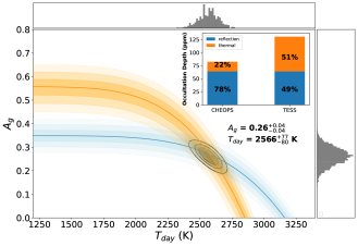
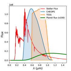
Figure 5: Dayside reflection and emission brightness contributions. Left: Geometric albedo $(A_{g})$ as a function of the dayside brightness temperature for the estimated occultation depths in CHEOPS (blue) and TESS (red). The decreasing intensity of the colour shades corresponds to the 1 $\sigma$, 2 $\sigma$, and 3 $\sigma$ uncertainties in the computation of $A_{g}$ for each $T_{\mathrm{day}}$. The overlapping region provides the true constraints on the two parameters represented by the posterior distribution in grey. The individual posteriors of $(A_{g})$ and $(T_{\mathrm{day}})$ are presented in the side panels. The resultant values are reported in the text. Subpanel: Reflection and emission contributions to the occultation depth of the CHEOPS and TESS passbands. The identical height of the reflection component reflects the assumption of $\alpha=1$. Right: Kurucz stellar model [$T_{eff}=9000$, $[Fe/H]=0$ and $logg=4.5$] along with the CHEOPS and TESS passband responses. The dayside planetary black-body flux (x100) is also plotted for a comparison with the stellar flux, $T_{day}=2600$ K.

Additionally, the same dataset can also be explained with alternative scenarios. If we break the identical $A_{g}$ assumption, but keep the same $T_{\mathrm{day}}$, then the maximum brightness temperature is $2857\begin{subarray}{c}+29\\ -25\end{subarray}$ K, which is equal to the maximum $T_{\mathrm{day}}$ associated with $\delta_{\mathrm{occ}}$ of TESS. This would imply $A_{g,\mathrm{TESS}}=0$ and $A_{g,\mathrm{CHEOPS}}=0.17\pm 0.03$ (i.e. entirely absorbing atmosphere in TESS band, and yet significantly reflective in the CHEOPS band). Furthermore, if we assume no reflection contribution whatsoever, then we need to give up the black-body assumption. This leads to maximum $T_{\mathrm{day}}$ associated with the observed $\delta_{\mathrm{occ}}$ of CHEOPS, $T_{\mathrm{day}}$ = $3162\begin{subarray}{c}+45\\ -47\end{subarray}$ K. Nevertheless, this scenario is less likely following Sect. 5.1.

Following Wong et al. (2021), we re-plotted the $A_{g}$ versus $T_{\mathrm{day}}$ for the sample of the hot Jupiters discussed in their paper along with the published CHEOPS results in Fig. 6. It is quite clear that there is a positive correlation between $A_{g}$ and $T_{\mathrm{day}}$ for HJ to UHJ in their work, with the exception of a few outliers like WASP-18b and WASP-33b. We observed a similar trend within the CHEOPS sample, thereby corroborating that UHJs tend to be more reflective compared to HJs. Although in comparison with the entire sample, the addition of the CHEOPS sample suggests a flattening of A_g for higher temperatures.

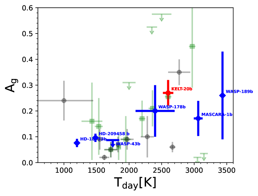
Figure 6: $A_{g}-T_{day}$ of several hot Jupiters following Wong et al. (2021). The black circles (Kepler-CoRoT) and the green squares (TESS) are taken directly from their sample. The blue diamonds correspond to the published values of the CHEOPS hot Jupiters (Krenn et al. 2023; Brandeker et al. 2022; Scandariato et al. 2022; Pagano et al. 2023; Hooton et al. 2022; Deline et al. 2022). The red diamond is from this work on KELT-20 b.

5.2.2 Bond albedo

The Bond albedo ($A_{B}$, Bond 1861) or the spherical bolometric albedo Mallama (2017) is a measurement of the fraction of the total power of the incident radiation that is scattered back at all wavelengths and all phase angles. It provides a measure of a planet’s energy budget that further provides information about its atmospheric composition and the overall thermal properties (Schwartz & Cowan 2015). To convert a geometric albedo into a Bond albedo, we need information about the planet’s reflectance spectrum, scattering phase function, and spatial inhomogeneity (Hanel et al. 2003). In practice, the geometric albedo is related to the spherical albedo through the phase integral q (i.e. the integral of the scattering phase function), which gets translated to the Bond albedo through the relation

$$A_{\rm B}=\frac{\int_{0}^{\infty}q(\lambda)A_{\rm g}(\lambda)I_{\star}(\lambda)d\lambda}{\int_{0}^{\infty}I_{\star}(\lambda)d\lambda},$$ (8)

where $I_{\star}$ is the wavelength-dependent stellar intensity. For a Lambert sphere, q=2/3, and assuming a geometric albedo independent of wavelengths (i.e. a flat albedo spectrum), we obtain $A_{B}=3/2A_{g}$. This formalism has been the norm during the Kepler and the Spitzer era.

Following Cowan & Agol (2011), the effective dayside ($T_{d}$) and nightside temperatures ($T_{n}$) can be expressed in terms of the bond albedo $A_{B}$ and the heat re-circulation efficiency $\epsilon$ that parametrises the heat flow from the day side to the night side (Eq. 9 and 10):

$$T_{d}=T_{\rm eff}\sqrt{\frac{R_{\star}}{a}}\left(1-A_{B}\right)^{\frac{1}{4}}\left(\frac{2}{3}-\frac{5}{12}\epsilon\right)^{\frac{1}{4}},$$ (9)

$$T_{n}=T_{\rm eff}\sqrt{\frac{R_{\star}}{a}}\left(1-A_{B}\right)^{\frac{1}{4}}\left(\frac{\epsilon}{4}\right)^{\frac{1}{4}}.$$ (10)

Here $\epsilon=0$ indicates instantaneous re-radiation or no re-circulation of heat from the day side to the night side, while $\epsilon=1$ means perfect heat re-circulation. In the previous section we estimated the observed brightness temperature of the planet $T_{\mathrm{day}}$ within the CHEOPS-TESS passband. The best-fit planetary spectral energy distribution (SED) obtained from Sect. 5.1 equates to a thermal flux with an irradiation temperature of $2618^{+35}_{-40}$ K. We use this as the effective temperature of the planetary day side $T_{d}$. We therefore invert Eq. 9 to provide constraints on the associated bond albedo $A_{B}$ with varying $\epsilon$, as shown in Figure 7. The solid black line represents the $A_{B}$ value with varying $\epsilon$, while the dashed grey lines are the 16${th}$ and 84${th}$ percentiles. The orange and light blue span represents the constraints on the bond albedo following the Lambertian scattering law (i.e. $q=3/2$) and the 100$\%$ back-scattering law (i.e. $q=1$), respectively. These estimates are computed using the $A_{g}$ value derived in Sect. 5.2.1.

Figure 7: Parameters determining planetary energy distribution under radiative equilibrium. Top right: Bond albedo plotted as a function of the heat re-circulation efficiency for the effective dayside temperature $T_{\rm d}$. Bottom left: Respective posteriors of $A_{B}$ and $\epsilon$ from the overlapping region, which are then used to compute the nightside temperature. The values in the label correspond to the orange posteriors, while the light blue posteriors are shown only for comparison.

For the extreme case of inefficient heat re-circulation (i.e. $\epsilon=0$), we derive an upper limit on the bond albedo of $0.45\pm 0.07$. We note that this does not make any assumptions regarding the phase integral ($q$), which relates the geometric albedo to the Bond albedo. We can however use our derived value of $A_{g}$ within the CHEOPS-TESS passbands to further constrain the limits on $A_{B}$ and $\epsilon$. Following the same approach as Schwartz & Cowan (2015), we use Eq. 8 and consider the two limits on the phase integral (i.e. q=3/2, Lambert scattering, and q=1, 100$\%$ back-scattering). As we have no information of the geometric albedo in the UV/FUV wavelength ranges, we assume a constant $A_{g}$ equal to that measured in the optical. Figure 7 shows the posterior distribution of the $A_{B}$, $\epsilon$ along with the dayside and nightside temperatures for the two limiting scenarios.

We report the values corresponding to the flat $A_{g}$ with the planet following Lambertian scattering, which gives $A_{B}=0.36^{+0.04}_{-0.06}$, $\epsilon$ = $0.14^{+0.13}_{-0.10}$ and the nightside temperature $T_{n}=1266^{+259}_{-330}$ K. The uncertainties are propagated from the error estimates on the stellar effective temperature from Table 1 and the semi-major axis from Table 4. The low value of $\epsilon$ indicates weak heat re-circulation, while the average nightside temperature will result in emission signatures that too low to be detectable in the TESS phase curves, which corroborates well with the nightside emission estimates that is consistent with zero. If a more asymmetric scattering law is assumed ($q<3/2$), a combination of smaller $A_{B}$ and higher $\epsilon$ would also be possible. In the limiting case of $q=1$ or $A_{B}=A_{g}$, we obtain $\epsilon$ as $0.38^{+0.09}_{-0.07}$, while the nightside temperature $T_{n}$ is $1708^{+113}_{-93}$ K.

5.3 Atmospheric variability

In addition to a precisely constrained geometric albedo of the day side of KELT-20 b , our data also shows a tentative detection of temporal variability in the occultation depth (see Sect. 4.2), which most plausibly can be attributed to the varying flux from the planetary day side. Prior reports of variability in a hot-Jupiter atmosphere were announced for HAT-P-7 b (Armstrong et al. 2016) and WASP-12 b Wong et al. (2022). For HAT-P-7 b, variability was observed in the phase curve shape, interpreted as changes in the location of the brightest point. Although this interpretation was later challenged and attributed to stellar super-granulation (Lally & Vanderburg 2022). The behaviour of KELT-20 appears to differ, showing changes in the occultation depth itself which can be best illustrated when we analyse its variability within the first four visits of CHEOPS in conjunction with the simultaneous TESS Sector 40 and 41 occultations.

If we only consider the TESS Sector 40 observations combined with the first two simultaneous occultation observations of CHEOPS, we obtained the respective depths of 102$\pm$22 and 62$\pm$9 ppm for TESS and CHEOPS. Following the method described in Section 5.2.1, these values yield a grey-sky geometric albedo of 0.16$\pm$0.1. Conversely, if we consider only TESS Sector 41 and the later two occultations of CHEOPS (i.e. visits 3 and 4), then the respective depths are 149$\pm$34 and 103$\pm$10 ppm. This scenario yields a higher grey-sky geometric albedo of 0.31$\pm$0.1. Driven by the less discrepant TESS measurements, the derived average dayside temperatures remain compatible within 1 $\sigma$. This suggests that a brightness variability through reflectivity, as expected from varying cloud cover, rather than temperature, is at play.

Understanding the cloud coverage and variability requires understanding the underlying 3D cloud coverage. Recently, Helling et al. (2023) provided an extensive grid of 3D cloudy models for warm to ultra-hot Jupiters. KELT-20 b is an ultra-hot Jupiter that corresponds best to the 2200 K hot 3D case around an F-type star in their Figure 5. Such a planet is expected to have a partly cloudy morning terminator because the relatively slow rotation of the tidally locked planet of 3.5 days still promotes the formation of a strong super-rotating jet, which carries cloud particles from the night side towards the day side, that can cover up to 30 degrees of the morning terminator with thick clouds in the steady-state climate. Therefore, the cloud coverage on the dayside limbs on such ultra-hot Jupiters is mostly determined by the strength of the super-rotating wind jet.

The location of the hot spot shift is also highly sensitive to the strength of the super-rotating wind jet. We note, however, that compared to hot Jupiters like HD 209458 b with an effective dayside temperature $T_{\mathrm{d}}=1500$ K, the hot spot shift is very much reduced for an ultra-hot Jupiter with $T_{\mathrm{d}}>2000$ K because the radiative timescales are proportional to $\propto T^{-3}$, and thus become very short compared to the dynamical timescale. In other words, the hot air on the day side cools off faster as it is transported eastwards towards the night side.

It has been pointed out again by Helling et al. (2023) that such a planet is also highly thermally ionised at the day side (their Figure 14). Several authors (Komacek & Showman 2020; Beltz et al. 2022; Hindle et al. 2021) suggest that the coupling of ionised flow with the planetary magnetic fields can then lead to drastic changes in the 3D wind structure, sometimes entirely suppressing the super-rotating wind jet. A suppressed super-rotating wind jet results in a reduction of the cloud influx towards the dayside hemisphere and a disappearance of any hot-spot offset on such a highly irradiated planet.

Additionally, changes in the interior heat flux can also lead to fluctuations in the strength of the super-rotating wind jet and thus the morning cloud and hot spot shift (Carone et al. 2020; Schneider et al. 2022; Komacek et al. 2022). Thus, a combination of magnetic field interactions and possible interior effects can lead to variations in the occultation depth, as the hot spot is shifted more or less away from the substellar point, and in the planet’s albedo, due to the accompanying morning cloud variability.

Next to the low S/N, distinguishing between reflection and emission in the TESS band is difficult as it is impractical to incorporate two degenerate phase amplitude terms to account for reflection and emission separately. Therefore, a single phase offset term would have to account for both the individual phase variations. A phase offset consistent with zero can still involve super-rotating jets accompanied by morning cloud because of the complementarity of the reflection bright spot and the emissive hot spot in the phase curve. Compared to TESS, the CHEOPS occultations are more sensitive towards the reflected stellar light that accounts for around three-fourths of the total planetary optical dayside flux (Fig. 5 inset). While CHEOPS data cover occultations only and are thus not well suited to deriving phase curve peak offsets, the object might possess a phase offset in the optical due to enhanced reflection from clouds near the dayside terminator. Future high-precision phase curves of KELT-20 b at bluer wavelengths can shed more light onto this aspect.

Unlike HAT-P-7 b (Armstrong et al. 2016), the variability in the occultation depth cannot be attributed to super-granulation in the host-star (Lally & Vanderburg 2022). Because KELT-20  is an A dwarf star, it does not possess a convective layer, and as a result it is less likely that it exhibits granulation signatures. Thus, KELT-20 b is ideally amenable to study 3D weather and variability due to interactions between a highly ionised day side and the planetary magnetic field.

5.4 Spin-orbit alignment

Our gravity-darkening analysis (Section 3.2, Table 4) confirms the previous Doppler tomography measurements (Table 5) that KELT-20 b orbits in a plane that is misaligned from the stellar equatorial plane by at most a few degrees. As Barnes et al. (2011) point out, there is a four-way degeneracy in the value of $\lambda$ obtained from gravity-darkened transits; we must rely on the Doppler tomography results to exclude the retrograde solutions.

We see no evidence for nodal precession in KELT-20  unlike in the Kepler-13 (Szabó et al. 2012, 2020) and WASP-33 (Johnson et al. 2015; Watanabe et al. 2022; Stephan et al. 2022) systems, for instance, where the nodal precession is fast enough to cause measurable changes in the impact parameter of the transits over a relatively short baseline. This is in line with theoretical expectations (Iorio 2011) given that the KELT-20 system has a near-zero obliquity.

Table 5: Comparison of the sky-projected obliquity values.

$\lambda$ /degrees	Source
$3.4\pm 2.1$	Lund et al. (2017)
$0.6\pm 4.0$	Talens et al. (2018)
$1.6\pm 3.1$	Hoeijmakers et al. (2020a)
$3.9\pm 1.1$	CHEOPS∗
$9\pm 1$	TESS∗

^∗ Only the prograde solutions for $\lambda$ are listed here, although a retrograde orbit cannot be excluded by the light curves alone.

6 Conclusion

In this work, we present a detailed optical picture of the KELT-20 system. Using CHEOPS observations of five transits and seven occultations of KELT-20 b, as well as four Sectors worth of TESS data, we obtained a precise planetary radius along with a more than $3\leavevmode\nobreak\ \sigma$ detection of the planet’s obliquity and constraints on the star–planet alignment. The CHEOPS photometry found an aligned orbit for KELT-20 b, which is in contrast to previous CHEOPS studies that have found strongly inclined orbits for planets orbiting other A-type stars Lendl et al. (2020); Hooton et al. (2022); Deline et al. (2022). At the same time, we also probed the atmospheric properties of this UHJ.

We used the emission spectrum obtained with HST and Spitzer from the literature to provide a picture of the UHJ dayside thermal profile. We confirmed the observation of temperature inversion in the atmosphere of KELT-20 b. Additionally, with the help of TESS photometry in synergy with CHEOPS  we provide strong constraints on the geometric albedo at $0.26\pm 0.04$ and the dayside brightness temperature at $2566^{+77}_{-80}$ K. The high geometric albedo corroborates a known trend of strongly irradiated planets being more reflective. Such a combination of the $A_{g}-T_{day}$ pair results in a reflection emission contribution of 3:1 and 1:1 to the occultation depth for CHEOPS and TESS, respectively. This further leads to informative constraints on the planetary bond albedo and the heat re-circulation efficiency. The day side is too hot to form clouds, and therefore the precise nature of the high geometric albedo could either be attributed to strong scattering by atoms or ions on the day side or by reflective clouds around the planet’s terminator. We explored the possible scenarios of cloud reflections.

The high precision of the CHEOPS occultations also reveals signs of variability in the occultation depth, suggesting variable brightness of the planetary day side. As CHEOPS measurements are dominated by reflected light, the temporal variability in occultation depth could be attributed to variations in the extent of advected nightside clouds onto the planetary limbs (see e.g. Helling et al. 2021; Adams et al. 2022 for a discussion on the impact of clouds at the limbs of hot Jupiters and how these may affect dayside albedos). These authors note, however, that their simple model cannot address the variations seen to date. Thus, clearly more work is needed to investigate the precise origin of the variations that our CHEOPS measurements revealed. A combination of magnetic field interactions and possible interior feedback can also lead to such a variation. Spectroscopic occultation or phase curve observations of KELT-20 b especially in the UV/FUV will shed more light on the magnitude and nature of reflective sources in this UHJ. While spectroscopic observations in the infrared can shed more light on the energy budget and the physical processes governing this planet, making it ideally suited for follow-up observations with HST, JWST, and eventually ARIEL.

Appendix A CHEOPS observations of KELT-20 b 

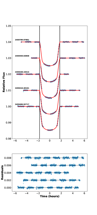
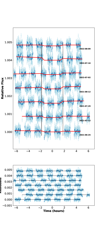
Figure 8: Individual CHEOPS transits (left) and occultations (right) of KELT-20 b. The solid red line is the best-fit model, while the blue and light blue points represent the binned and unbinned light curves, respectively. The numbers in the figure represent the BJD time stamp of individual transit epochs. The residuals are shown in the bottom panel.

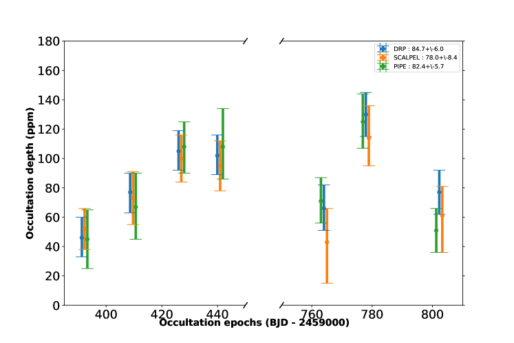
Figure 9: Occultation depth measurements of KELT-20 b of the seven CHEOPS observations. The three sets of measurements correspond to the three data extraction techniques discussed in Sect. 2

Table 6: Best-fit parameters of the individual transit fits of CHEOPS

Visit ID	$T_{\mathrm{epoch}}$	$R_{p}/R_{\star}$	$b$	$\rho_{\star}$ [solar]	$q_{1}$	$q_{2}$
TG000401	2459406.927174$\pm$0.000024	0.11573${}^{+0.00030}_{-0.00031}$	0.516$\pm$0.007	0.458$\pm$0.005	0.278${}^{+0.053}_{-0.047}$	0.289${}^{+0.113}_{-0.094}$
TG000402	2459410.4016${}^{+0.0366}_{-0.0393}$	0.11571${}^{+0.00033}_{-0.00032}$	0.504$\pm$0.016	0.472$\pm$0.016	0.231${}^{+0.028}_{-0.026}$	0.36${}^{+0.063}_{-0.057}$
TG0001001	2459438.194141${}^{+0.000032}_{-0.000033}$	0.11509${}^{+0.00039}_{-0.00040}$	0.501$\pm$0.011	0.471$\pm$0.007	0.301${}^{+0.047}_{-0.042}$	0.268${}^{+0.067}_{-0.058}$
TG0001002	2459459.038579${}^{+0.000251}_{-0.000244}$	0.11588${}^{+0.00061}_{-0.00060}$	0.527${}^{+0.027}_{-0.031}$	0.452${}^{+0.031}_{-0.028}$	0.259${}^{+0.041}_{-0.038}$	0.300${}^{+0.082}_{-0.067}$
TG000801	2459789.078614$\pm$0.00044	0.11587${}^{+0.00032}_{-0.00037}$	0.502$\pm$0.003	0.467${}^{+0.029}_{-0.025}$	0.310${}^{+0.037}_{-0.035}$	0.255${}^{+0.052}_{-0.057}$

Appendix B TESS observations of KELT-20 b 

Table 7: TESS: Best-fit transit and phase curve free parameters of KELT-20 b.

Parameter	Sector 14	Sector 40	Sector 41	Sector 54
$T_{\mathrm{epoch}}$ [TJD]	$1694.736671\pm 0.000062$	$2403.453023\pm 0.000038$	$2434.720013\pm 42$	$2771.707828\pm 0.000083$
Period* [d]	$3.474078^{+0.000029}_{-0.000030}$	$3.474106\pm 0.000016$	$3.474086\pm 0.000018$	$3.474101^{+0.000018}_{-0.000019}$
$\rho_{\star}$ [solar]	$0.470\pm 0.006$	$0.458\pm 0.006$	$0.461\pm 0.007$	$0.454\pm 0.007$
$R_{p}/R_{\star}$ [$\%$]	$11.581^{+0.036}_{-0.039}$	$11.569^{+0.026}_{-0.027}$	$11.549\pm 0.030$	$11.603^{+0.026}_{-0.031}$
$b$	$0.508^{+0.008}_{-0.009}$	$0.508\pm 0.008$	$0.513\pm 0.009$	$0.525^{+0.008}_{-0.009}$
$q_{1}$	$0.146^{+0.042}_{-0.032}$	$0.126^{+0.021}_{-0.019}$	$0.146^{+0.024}_{-0.022}$	$0.125^{+0.024}_{-0.019}$
$q_{2}$	$0.268^{+0.099}_{-0.10}$	$0.427^{+0.102}_{-0.086}$	$0.326^{+0.0.091}_{-0.078}$	$0.393^{+0.107}_{-0.098}$
$A_{\mathrm{day}}$ [ppm]	$107\pm 30$	$102\pm 22$	$149\pm 34$	141${}^{+43}_{-46}$
$\log(h)$	$-6.44^{+0.79}_{-0.35}$	$-8.13^{+0.13}_{-0.11}$	$-8.06^{+0.09}_{-0.08}$	$-8.52^{+0.10}_{-0.09}$
$\log(l)$	$2.57^{+0.60}_{-0.46}$	$-0.58^{+0.13}_{-0.12}$	$-1.34\pm 0.09$	$-1.56^{+0.16}_{-0.15}$
Jitter [ppm]	$287\pm 5$	$178\pm 3$	$177\pm 4$	$171\pm 5$

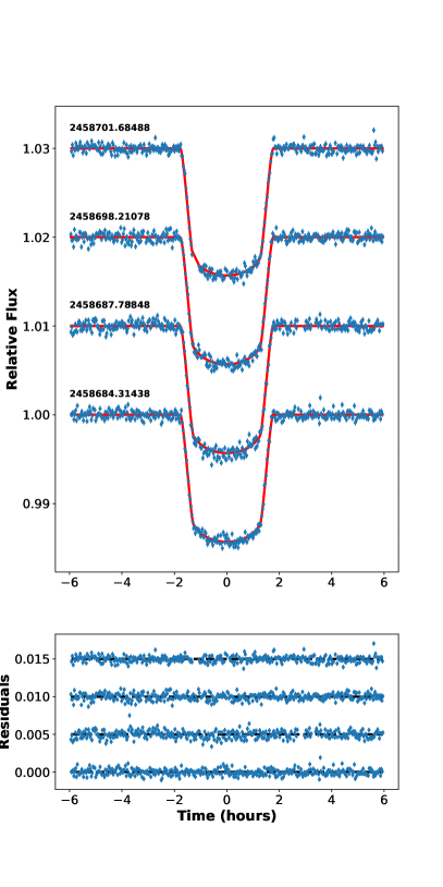
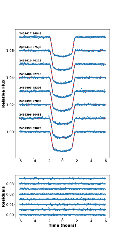
Figure 10: Individual transits of KELT-20 b observed with TESS. The solid red line is the best-fit model, while the blue and light blue points represent the binned and unbinned light curves respectively. The numbers represent the BJD time stamp of individual transit epochs. The residuals are shown in the bottom panel. Left: All transits of sectors 14. Right: All transits of sector 40.

Figure 11: Same as in Fig. 10, but for sectors 41 and 54.

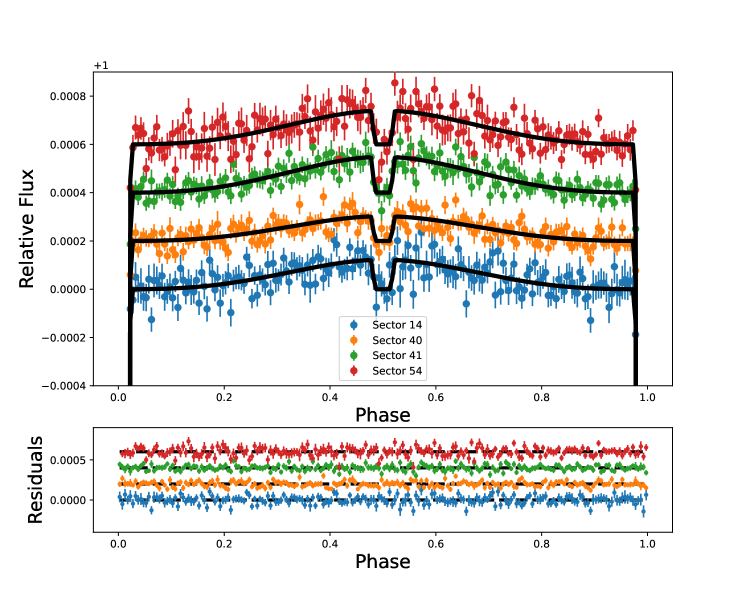
Figure 12: Individual sector-wise TESS phase curves of KELT-20 b. The variation in the occultation depth is somewhat apparent between Sectors 40 and 41. The sector-wise occultation depths are $123^{33}_{34}$, 102$\pm$34, 149$\pm$35, and $141^{+43}_{-46}$ ppm for sectors 14, 40, 41, and 54 ppm, respectively. The corresponding residuals are in the bottom panel.

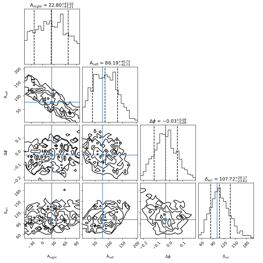
Figure 13: Posteriors of the model that includes the phase offset and the nightside flux as free parameters for TESS Sector 40. $\Delta\phi$ varies between 0 and 1 ($360^{\circ}$). Both $A_{night}$ and $\Delta_{\phi}$ are consistent with zero, and the occultation depth measurement is the same as that measured when they are fixed to zero (see Table 7).

Appendix C Derived parameters

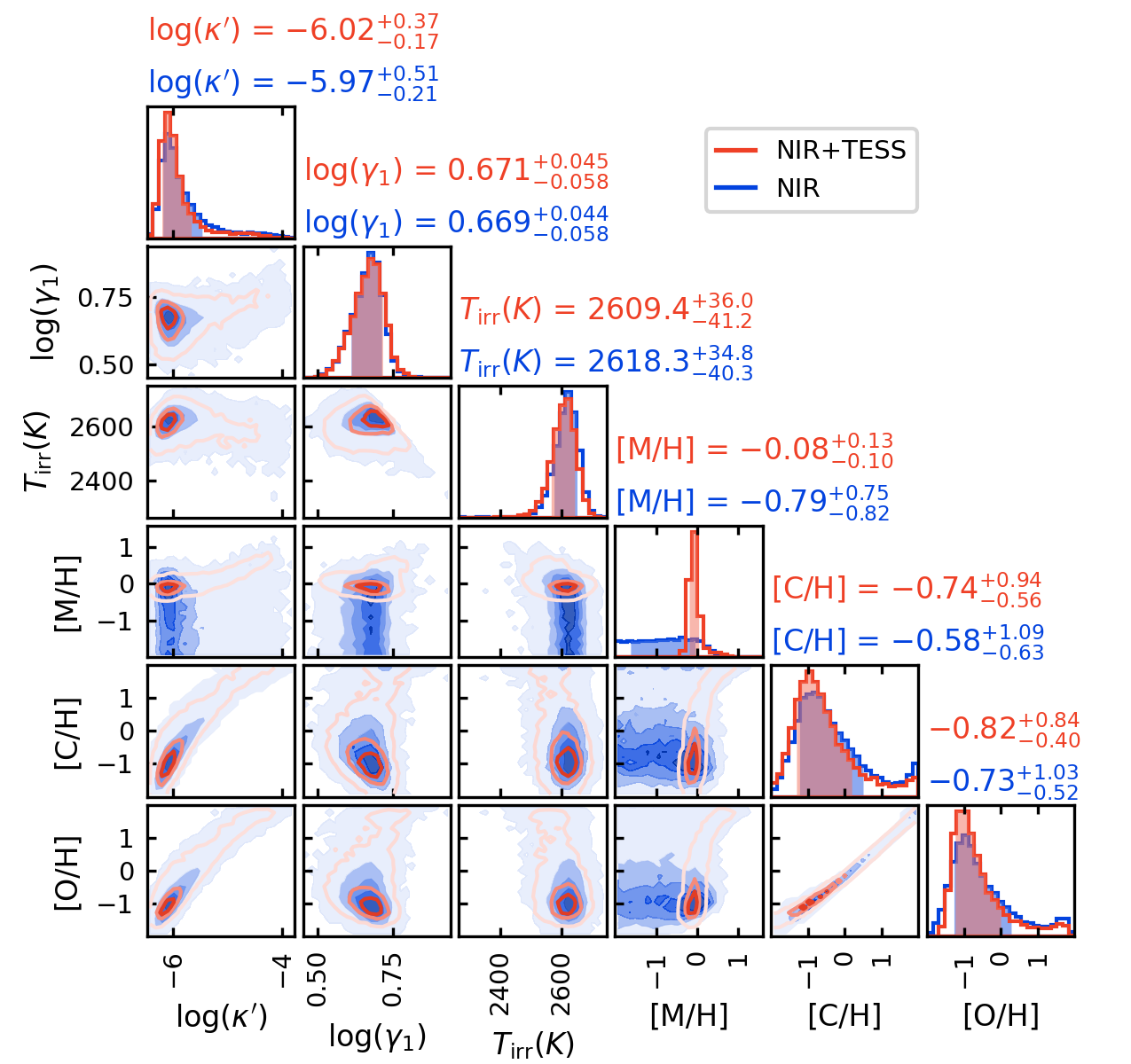
Figure 14: Posterior distributions for our KELT-20 b atmospheric retrievals constrained by the NIR occultations (HST and Spitzer, blue) and the NIR+TESS occultations (red). The reported values at the top of each marginal posterior denote the median of the distribution and the boundaries of the central 68% percentile (i.e. the 1$\sigma$ credible intervals). The shaded areas in the marginal histograms denote the span of the credible intervals.

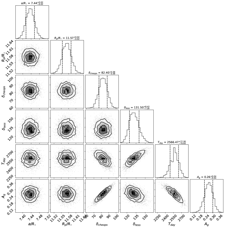
Figure 15: Posterior distribution of the CHEOPS and TESS eclipse depths in ppm along with the planetary fit parameters $R_{p}/R_{\star}$ [$\%$] and a/$R_{\star}$ from the light curve fitting are used to create the posteriors on the dayside brightness temperature and geometric albedo (for reference, see Sect. 5).