Parameter-Agnostic Optimization under Relaxed Smoothness

Abstract

Tuning hyperparameters, such as the stepsize, presents a major challenge of training machine learning models. To address this challenge, numerous adaptive optimization algorithms have been developed that achieve near-optimal complexities, even when stepsizes are independent of problem-specific parameters, provided that the loss function is $L$-smooth. However, as the assumption is relaxed to the more realistic $(L_{0},L_{1})$-smoothness, all existing convergence results still necessitate tuning of the stepsize. In this study, we demonstrate that Normalized Stochastic Gradient Descent with Momentum (NSGD-M) can achieve a (nearly) rate-optimal complexity without prior knowledge of any problem parameter, though this comes at the cost of introducing an exponential term dependent on $L_{1}$ in the complexity. We further establish that this exponential term is inevitable to such schemes by introducing a theoretical framework of lower bounds tailored explicitly for parameter-agnostic algorithms. Interestingly, in deterministic settings, the exponential factor can be neutralized by employing Gradient Descent with a Backtracking Line Search. To the best of our knowledge, these findings represent the first parameter-agnostic convergence results under the generalized smoothness condition. Our empirical experiments further confirm our theoretical insights.

1 Introduction

We consider the unconstrained optimization problem

$$\min_{x\in\mathbb{R}^{d}}F(x),$$ (1)

where $F\colon\mathbb{R}^{d}\to\mathbb{R}$ may be non-convex and admits access to unbiased stochastic gradients. This setting has been extensively studied due to its prevalence in modern machine learning and data-driven optimization (Bottou et al.,, 2018).

When the objective function $F$ is $L$-smooth, i.e., $F$ has $L$-Lipschitz gradients, the problem is well-explored. For the goal of finding an $\varepsilon$-stationary point, lower bounds have been established, notably by Arjevani et al., (2022), setting a limit of $\Omega{\left({L\Delta_{1}\sigma^{2}}{\varepsilon^{-4}}\right)}$ for stochastic first-order methods. Here $\sigma$ denotes the variance of the stochastic gradient and $\Delta_{1}$ the initialization gap. Stochastic Gradient Descent (SGD) achieves this complexity but with stepsizes depending on problem parameters like $L$ (Ghadimi and Lan,, 2013). Remarkably, several algorithms such as AdaGrad-Norm, oblivious to problem parameters, are recently proven to achieve a nearly rate-optimal complexity $\widetilde{\mathcal{O}}{\left(\varepsilon^{-4}\right)}$, up to the dependency on problem parameters and logarithmic factors (Faw et al.,, 2022; Yang et al.,, 2022). We call algorithms with this characteristic parameter-agnostic, and parameter-dependent otherwise.

However, Zhang et al., 2020b highlight that not all machine learning applications adhere to the $L$-smoothness assumption. Their experiments in language modeling tasks revealed that the norm of the Hessian is not uniformly upper-bounded as required by $L$-smoothness. Rather, it may increase affinely with the gradient norm. To bridge the gap between theory and this observation, they introduced a more general smoothness condition termed ($L_{0},L_{1}$)-smoothness:

$$\left\lVert\nabla^{2}F{\left(x\right)}\right\rVert\leq L_{0}+L_{1}\left\lVert{{\nabla F}{\left(x\right)}}\right\rVert.$$

This condition has since been further validated in various machine learning tasks (Zhang et al., 2020a, ; Crawshaw et al.,, 2022).

In light of this more realistic smoothness assumption, a substantial body of literature has emerged. The nearly rate-optimal complexity $\widetilde{\mathcal{O}}{\left(\varepsilon^{-4}\right)}$ has been established for various algorithms, including SGD (Li et al., 2023b, ), Clipped SGD (Zhang et al., 2020b, ; Zhang et al., 2020a, ), Normalized SGD (Zhao et al.,, 2021), AdaGrad-Norm (Faw et al.,, 2023; Wang et al.,, 2023) and ADAM (Li et al., 2023a, ). Yet, all of these algorithms require prior information of the problem, such as the values of $L_{0}$ and $L_{1}$. Notably, unlike the $L$-smooth setting, AdaGrad-Norm may diverge without access to $L_{1}$ (Wang et al.,, 2023), shedding its fully parameter-agnostic nature. This dependence on problem parameters poses a significant challenge as these parameters are usually unknown in practical applications, necessitating resource-intensive tuning (Ward et al.,, 2019). These observations culminate in the pressing question:

Is there an algorithm that converges with near-optimal complexity, without having access to any problem parameters in the ($L_{0}$, $L_{1}$)-smoothness setting?

With the growing interest in the development of parameter-agnostic algorithms, a fundamental trade-off becomes evident: while these algorithms demand less prior knowledge about the problem, they may also offer weaker convergence guarantees. For instance, under $L$-smoothness, SGD with decaying stepsizes ${\eta}_{t}=\nicefrac{{\eta}}{{\sqrt{t}}}$ achieves the near-optimal complexity $\widetilde{\mathcal{O}}{\left(L\Delta_{1}\sigma^{2}\varepsilon^{4}\right)}$ when $\eta$ is selected using knowledge of problem parameters (Ghadimi and Lan,, 2013). Without this information, however, using the same stepsizes has been shown to suffer from a lower bound of $\Omega{\left(\eta^{-4}L^{-2}e^{\nicefrac{{{\left(\eta L\right)}^{2}}}{{8}}}\varepsilon^{-4}\right)}$, even in the deterministic setting (Yang et al.,, 2022).

This gap underscores the need to differentiate between parameter-agnostic and parameter-dependent algorithms when establishing lower bounds to truly grasp the potential of parameter-agnostic algorithms. However, the existing lower bound framework is constructed in a way that implicitly allows algorithms to have access to problem-specific parameters. This shortcoming raises the second key question that this paper seeks to address:

Can we develop a lower bound framework that distinguishes between parameter-agnostic and parameter-dependent algorithms?

1.1 Our Contributions

To tackle these challenges, this work makes the following contributions:

1. We show that, under the relaxed ($L_{0}$, $L_{1}$)-smoothness assumption, Normalized Stochastic Gradient Descent with Momentum (NSGD-M), as introduced by (Cutkosky and Mehta,, 2020), converges with a nearly rate-optimal complexity of $\widetilde{\mathcal{O}}{\left(\varepsilon^{-4}\right)}$ without any prior knowledge of the problem parameters. However, it results in an exponential dependency on $L_{1}$, which vanishes when the stepsize is informed by $L_{1}$. Furthermore, we prove that this exponential dependency can also be avoided in the deterministic setting using Gradient Descent (GD) with Backtracking Line Search, resulting in a complexity of $\mathcal{O}{\left({\left(L_{0}\Delta_{1}+L_{1}^{2}\Delta_{1}^{2}\right)}\varepsilon^{-2}\right)}$. To the best of our knowledge, these are the first parameter-agnostic convergence results in the ($L_{0},L_{1}$)-smoothness setting.

2. We provide a novel framework for lower bound analysis tailored to parameter-agnostic algorithms. Within this framework, we show that the exponential term in $L_{1}$ is indispensable for a class of Normalized Momentum Methods, including NSGD-M, when the problem parameters are unknown. This framework distinctly delineates the parameter-agnostic setting from the parameter-dependent setting, in which NSGD-M does not suffer from the exponential term. Additionally, it suggests that the ($L_{0},L_{1}$)-smoothness setting may be more challenging than the $L$-smoothness setting.

1.2 Related Work

Parameter-Agnostic Algorithms.

If the objective function is $L$-smooth, convergence results for SGD are typically contingent upon stepsizes being less than $\nicefrac{{2}}{{L}}$ (Bottou et al.,, 2018). In the deterministic setting, GD with a constant stepsize that does not satisfy this threshold may diverge (Nesterov,, 2018). However, this can be rectified using a Backtracking Line Search (Armijo,, 1966; Nocedal and Wright,, 1999), which does not rely on knowing problem parameters, and achieves an optimal complexity of $\mathcal{O}(\epsilon^{-2})$. Conversely, in the stochastic setting, Vaswani et al., (2022) highlighted that line search techniques might not always converge. SGD with a parameter-agnostic diminishing stepsize of $\nicefrac{{1}}{{\sqrt{t}}}$ still reaches a near-optimal complexity of $\widetilde{\mathcal{O}}(\epsilon^{-4})$, though it introduces an inescapable exponential term in $L$ (Yang et al.,, 2023). Various adaptive methods, such as AdaGrad (Duchi et al.,, 2011; McMahan and Streeter,, 2010), its variants AdaGrad-Norm (Streeter and McMahan,, 2010) and NSGD-M (Cutkosky and Mehta,, 2020), bypass this exponential term, even without knowledge of the problem parameters, as recently shown in (Faw et al.,, 2022; Yang et al.,, 2023). These adaptive methods are typically considered more robust to different problem parameters (Ward et al.,, 2019; Kavis et al.,, 2019), given their ability to tune algorithm hyperparameters dynamically during training. In convex optimization, certain algorithms can achieve (near-)optimal convergence rate without access to specific problem details (Lan,, 2015; Nesterov,, 2015; Levy et al.,, 2018). There is another line of research dedicated to “parameter-free” algorithms for online convex optimization (Orabona and Pal,, 2016; Cutkosky and Orabona,, 2018). However, this research emphasizes the optimal dependence on $\left\lVert x^{*}-x_{0}\right\rVert$, where $x^{*}$ is the predictor in the regret bound.

($L_{0},L_{1}$)-Smoothness.

Zhang et al., 2020b introduced the concept of ($L_{0},L_{1}$)-smoothness, defined by the following affine bound on the Hessian-norm: $\left\lVert\nabla^{2}F(x)\right\rVert\leq L_{0}+L_{1}\left\lVert{{\nabla F}{\left(x\right)}}\right\rVert$. The convergence of both GD and SGD was only recently established in this setting (Li et al., 2023b, ). However, their stepsizes require prior knowledge of $L_{0}$, $L_{1}$, and also the exact gradient norm of the initial point, which can be unavailable in stochastic settings. Clipped SGD (Zhang et al., 2020b, ), and its momentum-augmented counterpart (Zhang et al., 2020a, ), both demand knowledge of $L_{0}$ and $L_{1}$ for convergence. They attain an optimal complexity of $\mathcal{O}(\varepsilon^{-4})$ and are believed to improve over SGD in constants. Additionally, Zhang et al., 2020a also provided a convergence result for NSGD-M with constant stepsizes in the appendix. Their analysis does however make use of a stronger noise assumption and requires access to all parameters. Similar complexities have been established for Normalized SGD (Zhao et al.,, 2021), signed SGD (Crawshaw et al.,, 2022), AdaGrad-Norm (Faw et al.,, 2023; Wang et al.,, 2023), and ADAM (Li et al., 2023a, ; Wang et al.,, 2022). However, each of these methods requires prior knowledge of problem-specific parameters. Notably, in stark contrast to the $L$-smooth setting, even AdaGrad-Norm is not wholly parameter-agnostic. It risks divergence if the stepsize is not informed by $L_{1}$, despite the method generally demanding knowledge of fewer problem parameters than other algorithms (Wang et al.,, 2023).

Lower Bound Theory.

Lower bounds for seeking near-stationary points have been extensively studied within the $L$-smoothness setting. Nesterov, (2012) first addressed constrained optimization under box constraints. Subsequently, a seminal study by Carmon et al., (2020) established a tight lower bound of $\Omega{\left(\Delta_{1}L\varepsilon^{-2}\right)}$ for the deterministic setting. Arjevani et al., (2022) extended the results to the stochastic setting, introducing the $\Omega{\left(\Delta_{1}L\sigma^{2}\varepsilon^{-4}\right)}$ lower bound. Specific algorithms, such as SGD (Drori and Shamir,, 2020) and Newton’s method (Cartis et al.,, 2010), also have associated lower bounds. However, the algorithm classes considered by these lower bounds include algorithms with stepsizes that can depend on problem parameters, so they might not be tight in the parameter-agnostic setting. Vaswani et al., (2022) discovered that parameter-agnostic SGD with a specific exponentially decreasing stepsize suffers from an exponential dependence during its initial phase when minimizing strongly convex functions. Later, Yang et al., (2023) also derived a lower bound for SGD under a polynomially decreasing stepsize in the nonconvex setting. Yet the implications of the parameter-agnostic lower bound for a class of algorithms remain ambiguous. The aforementioned studies consider the function class of $L$-smooth functions, so they are also applicable to ($L_{0},L_{1}$)-smooth functions. In the realm of online convex optimization, Cutkosky and Boahen, (2016, 2017) have introduced a lower bound featuring an exponential term when the norm of the predictor and the Lipschitz constant are allowed to scale with the total number of iterations.

2 Preliminaries

Let us introduce basic notations, definitions and assumptions needed in the upcoming analysis.

Notation.

Throughout the paper, $d\in\mathbb{N}_{\geq 1}$ denotes the dimension of the variable to be optimized, $F\colon\mathbb{R}^{d}\to\mathbb{R}$ the objective and ${\nabla f}{\left(\cdot,\cdot\right)}$ the gradient oracle. We use the common convention that empty sums and products are given by their corresponding neutral element. The conic combination of ${{x}_{1},\dots,{x}_{n}}\in\mathbb{R}^{d}$ is denoted by $\operatorname{cone}{\left({{x}_{1},\dots,{x}_{n}}\right)}\coloneqq{\left\{\sum_{i=1}^{n}\lambda_{i}x_{i}\colon{{\lambda}_{1},\dots,{\lambda}_{n}}\geq 0\right\}}$. Functions that formally are not defined in a certain point, but have an continuous extension are to be understood as their extension. In particular, $\frac{e^{x}-1}{x}$ has the value $1$ in $x=0$.

Problem Setup.

Since finding a solution to (1) is computationally intractable (Nemirovskij and Yudin,, 1983), we aim to find an $\varepsilon$-stationary point. Furthermore we only allow access to a (possibly noisy) gradient oracle ${\nabla f}{\left(\cdot,\xi\right)}$ of ${\nabla F}$, where $\xi$ is a random vector. Due to this randomness, our specific goal is finding an approximate, random solution $x\in\mathbb{R}^{d}$ with $\mathbb{E}\left[\left\lVert{{\nabla F}{\left(x\right)}}\right\rVert\right]\leq\varepsilon$.

Building on established work in stochastic optimization (Ghadimi and Lan,, 2013; Arjevani et al.,, 2022), we employ the following two de-facto standard assumptions in various results of this study.

Assumption 1 (Lower Boundedness).

The objective function $F$ is lower bounded by $F^{*}>-\infty$.

Assumption 2 (Bounded Variance).

The gradient oracle is unbiased and has finite variance, i.e. there exists $\sigma\geq 0$ such that

1. $\mathbb{E}\left[{\nabla f}{\left(x,\xi\right)}\right]={{\nabla F}{\left(x\right)}}$, and

2. $\mathbb{E}\left[{\left\lVert{\nabla f}{\left(x,\xi\right)}-{\nabla F}{\left(x\right)}\right\rVert^{2}}\right]\leq\sigma^{2}$.

Instead of the traditional $L$-smoothness assumption, we adopt the weaker concept of ($L_{0},L_{1}$)-smoothness, as proposed by Zhang et al., 2020b . Following the work of Zhang et al., 2020a , we choose a definition that does not require the Hessian. This definition is therefore weaker than the original ($L_{0},L_{1}$)-smoothness assumption by Zhang et al., 2020b (, Definition 1).

Definition 3.

Let $L_{0},L_{1}\geq 0$ and $f\colon\mathbb{R}^{d}\to\mathbb{R}$ be a differentiable function. Then $f$ is called ($L_{0},L_{1}$)-smooth if for all $x,y\in\mathbb{R}^{d}$ and all $c>0$ with $L_{1}\left\lVert x-y\right\rVert\leq c$ it holds that

$$\left\lVert{\nabla f}{\left(x\right)}-{\nabla f}{\left(y\right)}\right\rVert\leq{\left(A_{0}{\left(c\right)}L_{0}+A_{1}{\left(c\right)}L_{1}\left\lVert{\nabla f}{\left(x\right)}\right\rVert\right)}\left\lVert x-y\right\rVert,$$

where $A_{0}{\left(c\right)}\coloneqq 1+e^{c}-\frac{e^{c}-1}{c}$ and $A_{1}{\left(c\right)}\coloneqq\frac{e^{c}-1}{c}$.

Assumption 4 (($L_{0},L_{1}$)-smoothness).

The objective function $F$ is ($L_{0},L_{1}$)-smooth.

Notably, the two definitions are equivalent if the objective function is twice differentiable as the following lemma shows. The proof can be found in Appendix A.

Lemma 1.

Let $F\colon\mathbb{R}^{d}\to\mathbb{R}$ be twice continuously differentiable and $L_{0},L_{1}\geq 0$. Then $F$ satisfies $\left\lVert\nabla^{2}F(x)\right\rVert\leq L_{0}+L_{1}\left\lVert{{\nabla F}{\left(x\right)}}\right\rVert$ if and only if $F$ is ($L_{0},L_{1}$)-smooth according to Definition 3.

3 Parameter-Agnostic Upper Bounds

In this section, we present the first parameter-agnostic convergence results on ($L_{0},L_{1}$)-smooth functions. In Section 3.1, we show that in the stochastic setting, NSGD-M (see Algorithm 1) achieves the nearly rate-optimal complexity of $\widetilde{\mathcal{O}}{\left(\varepsilon^{-4}\right)}$, even without access to problem-dependent parameters. However, this is accompanied by an undesirable exponential dependence on $L_{1}$. In Section 3.2 we show that in the deterministic setting, GD with Backtracking Line Search can avoid this exponential dependence, while still being parameter-agnostic.

3.1 Stochastic Setting

The convergence of NSGD-M occurs in two phases. In the initial adaptation phase, the algorithm accumulates error due to a large stepsize. Unfortunately, this error grows exponentially with $L_{1}$. This behaviour is intrinsic to NSGD-M and cannot be eliminated, as we will show in Section 4. Once the stepsize decreases below a threshold (which is polynomial in $L_{1}$), the algorithm transitions into a convergence phase. In this latter phase, the error decays at a rate of $T^{-\nicefrac{{1}}{{4}}}\log{\left(T\right)}$. The following Theorem 2 formalizes this behaviour, and the proof can be found in Section C.1.1.

Input : Starting point ${x}_{1}\in\mathbb{R}^{d}$, stepsizes ${\eta}_{t}>0$, moving average parameters ${\beta}_{t}\in[0,1)$

${m}_{0}\leftarrow 0$

for $t=1,2,\,\ldots$ do

       Indep. sample ${\xi}_{t}$ from the distribution of $\xi$.

       ${g}_{t}\leftarrow{\nabla f}{\left({x}_{t},{\xi}_{t}\right)}$

       ${m}_{t}\leftarrow{\beta}_{t}{m}_{{t-1}}+{\left(1-{\beta}_{t}\right)}{g}_{t}$

       ${x}_{{t+1}}\leftarrow{x}_{t}-\frac{{\eta}_{t}}{\left\lVert{m}_{t}\right\rVert}{m}_{t}$

      

end for

Algorithm 1 Normalized SGD with Momentum (NSGD-M) (Cutkosky and Mehta,, 2020)

Theorem 2 (Convergence of NSGD-M).

Assume ( (Lower Boundedness).), ( (($L_{0},L_{1}$)-smoothness).) and ( (Bounded Variance).). Furthermore, define the parameters ${\beta}_{t}\coloneqq 1-t^{-\nicefrac{{1}}{{2}}}$ and ${\eta}_{t}\coloneqq\frac{t^{-\nicefrac{{3}}{{4}}}}{7}$. Then NSGD-M with starting point ${x}_{1}\in\mathbb{R}^{d}$ satisfies

$$\frac{1}{T}\sum_{t=1}^{T}\mathbb{E}\left[\left\lVert{\nabla F}{\left({x}_{t}\right)}\right\rVert\right]\leq \ \widetilde{\mathcal{O}}{\left(\frac{\Delta_{1}e^{L_{1}^{2}}+\sigma+e^{L_{1}^{2}}L_{0}}{T^{\nicefrac{{1}}{{4}}}}\right)},$$

where $\Delta_{1}\coloneqq F{\left({{x}_{1}}\right)}-F^{*}$ is the initialization gap.

Since ($L_{0},L_{1}$)-smoothness includes $L$-smoothness as a special case, the lower bound of $\mathcal{O}(\varepsilon^{-4})$ to find an $\varepsilon$-stationary point is still applicable here. Theorem 2 implies an optimal complexity in $\varepsilon$ up to the logarithmic factor without any prior knowledge of the problem parameters, but it comes with the cost of an exponential term in $L_{1}$. The following corollary shows that this cost arises from the parameter-agnostic stepsize; that is, the exponential term disappears when the stepsize is informed by the value of $L_{1}$ only.

Corollary 3.

Under the assumptions of Theorem 2, define the parameters ${\beta}_{t}\coloneqq 1-t^{-\nicefrac{{1}}{{2}}}$ and ${\eta}_{t}\coloneqq\frac{t^{-\nicefrac{{3}}{{4}}}}{12L_{1}}$. Then NSGD-M with starting point ${x}_{1}\in\mathbb{R}^{d}$ satisfies

$$\frac{1}{T}\sum_{t=1}^{T}\mathbb{E}\left[\left\lVert{\nabla F}{\left({x}_{t}\right)}\right\rVert\right]\leq\widetilde{\mathcal{O}}{\left(\frac{L_{1}\Delta_{1}+\sigma+\frac{L_{0}}{L_{1}}}{T^{\nicefrac{{1}}{{4}}}}\right)},$$

where $\Delta_{1}\coloneqq F{\left({{x}_{1}}\right)}-F^{*}$ is the initialization gap.

These results indicate that NSGD-M is potentially more robust to hyper-parameter selection than other existing algorithms. In comparison, SGD necessitates knowledge of both $L_{0}$ and $L_{1}$, as well as the exact value of $\|\nabla f(x_{1})\|$ (Li et al., 2023b, ). Clipped SGD requires to know $L_{0}$ and $L_{1}$ (Zhang et al., 2020a, ), and even AdaGrad-Norm demands knowledge of $L_{1}$ (Faw et al.,, 2023; Wang et al.,, 2023). It is important to note that our analysis is significantly different from the previous analysis for NSGD-M in (Zhang et al., 2020a, ). The latter focused on constant stepsizes and momentum parameters determined by $L_{0}$, $L_{1}$, target accuracy $\varepsilon$, and variance $\sigma$. It furthermore made use of a stronger noise assumption.

3.2 Deterministic Setting

Given the prior results, one might naturally wonder if there exists any algorithm that can attain parameter-agnostic convergence without exponential dependence on $L_{1}$. The subsequent theorem confirms that this is indeed possible, at least in the deterministic setting. This is achieved by using Gradient Descent with a Backtracking Line-search (see Algorithm 2).

Input : Starting point ${x}_{1}\in\mathbb{R}^{d}$, Armijo parameters $\beta\in(0,1)$ and $\gamma\in(0,1)$

${\eta}_{0}\leftarrow 1$

for $t=1,2,\,\ldots$ do

       Choose $k\in\mathbb{N}$ minimal such that $\beta^{k}\leq{\eta}_{{t-1}}$ and $F{\left({x}_{t}-\beta^{k}{\nabla F}{\left({x}_{t}\right)}\right)}\leq F{\left({x}_{t}\right)}-\beta^{k}\gamma{\left\lVert{\nabla F}{\left({x}_{t}\right)}\right\rVert^{2}}$

       ${\eta}_{t}\leftarrow\beta^{k}$

       ${x}_{{t+1}}\leftarrow{x}_{t}-{\eta}_{t}{\nabla F}{\left({x}_{t}\right)}$

      

end for

Algorithm 2 GD with Backtracking Line Search

Theorem 4.

Assume ( (Lower Boundedness).)  and ( (($L_{0},L_{1}$)-smoothness).)  in the deterministic setting. Then GD with Backtracking Line Search (see Algorithm 2) with parameters $\beta,\gamma\in(0,1)$ satisfies

$$\frac{1}{T}\sum_{t=1}^{T}{\left\lVert{\nabla F}{\left({x}_{t}\right)}\right\rVert^{2}}\leq\frac{4L_{0}\Delta_{1}+14L_{1}^{2}\Delta_{1}^{2}}{\beta\gamma{\left(1-\gamma\right)}T},$$

where $\Delta_{1}\coloneqq F{\left({x}_{1}\right)}-F^{*}$.

This implies a complexity of $\mathcal{O}{\left({\left(L_{0}\Delta_{1}+L_{1}^{2}\Delta_{1}^{2}\right)}\varepsilon^{-2}\right)}$, which is optimal in the dependence of $\varepsilon$ and $L_{0}$ in the deterministic setting. The proof rests on the observation that GD with Backtracking Line Search is a descent algorithm and hence both the function value and gradient norm remain upper bounded along the trajectory. Consequently, the algorithm behaves as if it is addressing ${\left(L_{0}+L_{1}C\right)}$-smooth functions, where $C$ represents the gradient norm’s upper bound. The formal proof can be found in Section C.1.2. We have not extended our considerations to the stochastic setting for this algorithm, as a stochastic line search can potentially fail even under the stricter $L$-smoothness assumption (Vaswani et al.,, 2022).

4 Parameter-Agnostic Lower Bounds

In the previous section, we highlighted that the first provable parameter-agnostic algorithm, NSGD-M, comes at the cost of an exponential $L_{1}$-dependence. This naturally raises the question: Is such an undesirable term unavoidable for this class of algorithms? Since most existing lower bounds focus on the parameter-dependent setting — where hyper-parameters of algorithms can be set based on problem parameters — we begin by introducing the concept of lower bounds specifically designed for parameter-agnostic setting in Section 4.1. Subsequently, in Section 4.2, we utilize this concept to show that NSGD-M indeed suffers from an exponential dependence on $L_{1}$.

4.1 A Lower Bound Framework

To motivate the need for specific lower bounds for parameter-agnostic algorithms, let us consider the algorithm class $\mathcal{A}$ consisting of GD with all constant stepsizes $\{\eta:\eta>0\}$. Furthermore, we consider the well-studied function class comprising of $L$-smooth functions with initialization gap $F{\left({{x}_{1}}\right)}-F^{*}\leq\Delta_{1}$, denoted as $\mathcal{F}_{L,\Delta_{1}}$. A well-established lower bound for $\mathcal{A}$ to find an $\epsilon$-stationary point in this setting is $\Omega{\left(L\Delta_{1}\varepsilon^{-2}\right)}$, as demonstrated by the seminal work of Carmon et al., (2020). This lower bound is tightly matched by GD with a parameter-dependent stepsize smaller than $\nicefrac{{2}}{{L}}$, and hence cannot be improved. However, without knowledge of $L$, GD with constant stepsize generally fails to converge (Nesterov,, 2018). Thus, a parameter-agnostic notion of lower bounds would be more informative under this setting.

For simplicity, our discussion focuses on deterministic algorithms. However, this can be readily generalized to the stochastic setting by incorporating a stochastic oracle into the algorithm’s definition, as detailed in (Arjevani et al.,, 2022). Additionally, algorithms with a deterministic gradient oracle can be viewed as specific instances of their stochastic equivalents when there is no gradient noise. Consequently, the lower bounds established for deterministic algorithms are also applicable to their stochastic counterparts.

Definition 5 (Deterministic Algorithm (Carmon et al.,, 2020)).

We say that $A$ is a first order deterministic algorithm if it, given a differentiable function $f$, produces iterates of the form

$${x}_{t}=A_{t}{\left(f{\left({{x}_{1}}\right)},{\nabla f}{\left({{x}_{1}}\right)},\dots,f{\left({x}_{{t-1}}\right)},{\nabla f}{\left({x}_{{t-1}}\right)}\right)},$$

where $A_{t}$ is a (Lebesgue-) measurable mapping. We denote the set of all such algorithms as $\mathcal{A}_{\det}$.

It is important to note that an algorithm $A\in\mathcal{A}_{\det}$ is a function that takes a differentiable function as its argument and outputs a sequence in $\mathbb{R}^{d}$. When we mention an “algorithm with a specific stepsize scheme”, we are technically referring to a set of algorithms ${\left\{A_{\eta}\right\}}$, where $\eta$ serves as the hyperparameter of this stepsize scheme, and each distinct $\eta$ defines a unique algorithm.

In the following, we consider general parametrized function spaces, denoted by $\mathcal{F}_{\theta}$, where the parameter $\theta$ resides in a parameter space $\Theta\subseteq\mathbb{R}^{k}$. Specifically, in Section 4.2, we will use this concept with $\theta=(\Delta_{1},L_{0},L_{1})$. We use $\mathscr{F}_{\Theta}\coloneqq{\left\{\mathcal{F}_{\theta}\colon\theta\in\Theta\right\}}$ to denote a parametrized family of function spaces. For an algorithm class $\mathcal{A}\subseteq\mathcal{A}_{\det}$, existing lower bound literature usually considers the following challenge (Carmon et al.,, 2020): for any problem parameter $\theta\in\Theta$ and target accuracy $\epsilon>0$, find a lower bound for

$$\inf_{A\in\mathcal{A}}\sup_{f\in\mathcal{F}_{\theta}}T_{\varepsilon}{\left(A,f\right)},$$ (2)

where $T_{\varepsilon}{\left(A,f\right)}\coloneqq\inf{\left\{t\in\mathbb{N}_{\geq 1}\mid\left\lVert{\nabla f}{\left({x}_{t}\right)}\right\rVert\leq\varepsilon\right\}}$ denotes the number of iterations required for $A$ to reach an $\varepsilon$-stationary point of $f$. Importantly, the parameter $\theta$ is fixed for the function class $\mathcal{F}_{\theta}$ before taking the infimum over the algorithm class and supremum over the function class. This implicitly allows algorithms to adjust their hyperparameters based on $\theta$.

In contrast to the framework above, we propose the concept of parameter-agnostic lower bounds.

Definition 6 (Parameter-Agnostic Lower Bound).

Let $\mathcal{A}\subseteq\mathcal{A}_{\det}$ be an algorithm class and $\mathscr{F}_{\Theta}\coloneqq{\left\{\mathcal{F}_{\theta}\colon\theta\in\Theta\right\}}$ a parameterized family of function spaces. A function $g\colon(0,\infty)\times\Theta\to[0,\infty]$ is called a parameter-agnostic lower bound of $\mathcal{A}$ on $\mathscr{F}_{\Theta}$ if there does not exist an algorithm $A\in\mathcal{A}$ such that for all $\kappa>0$, there exists $\varepsilon_{0},\theta_{0}>0$ such that for all $\varepsilon\leq\varepsilon_{0},\theta\geq\theta_{0}$, $\sup_{f\in\mathcal{F}_{\theta}}T_{\varepsilon}{\left(A,f\right)}\leq\kappa g{\left(\varepsilon,\theta\right)}$. The comparisons of $\theta\in\Theta$ and scalars are to be understood component-wise.

In summary, the definition states that $g{\left(\varepsilon,\theta\right)}$ serves as a parameter-agnostic lower bound if no algorithm has a complexity that is “asymptotically better than” $g$. The performance of $A$ is therefore evaluated across all function spaces with $\theta$ large enough. This relation is formalized and elaborated upon in Appendix D. The conventional definition in Equation 2 on the other hand states that for any $\theta\in\Theta$ — which means the parameter is determined first — there does not exist an algorithm $A\in\mathcal{A}$ such that for all $\kappa>0$, $\sup_{f\in\mathcal{F}_{\theta}}T_{\varepsilon}{\left(A,f\right)}\leq\kappa g{\left(\varepsilon,\theta\right)}$. This implies that the the algorithm with the optimal hyperparameters for this $\theta$ is included in the assessment. Finally it should be noted that earlier parameter-agnostic lower bounds presented in (Yang et al.,, 2023; Vaswani et al.,, 2022) apply solely to a particular algorithm with a specified stepsize. Consequently, it is ambiguous how one might define a lower bound across a class of algorithms.

Additionally, Definition 6 also outlines a way to compare different algorithms within the parameter-agnostic framework by assessing their performance with asymptotically large $\theta$. We dive deeper into this possibility in Section D.2. This approach also facilitates a simplified technique for establishing $g$ as an parameter-agnostic lower bound of $\mathcal{A}$ on $\mathscr{F}_{\Theta}$.

Proposition 5.

If, for any algorithm $A\in\mathcal{A}$, there exist constants $\varepsilon_{0},\theta_{0},K>0$ such that

$$\forall\,\varepsilon\in(0,\varepsilon_{0}],\theta\geq\theta_{0}\colon\sup_{f\in\mathcal{F}_{\theta}}T_{\varepsilon}{\left(A,f\right)}\geq Kg{\left(\varepsilon,\theta\right)},$$

where $\theta\in\Theta$, then $g$ is a parameter-agnostic lower bound of $\mathcal{A}$ on $\mathscr{F}_{\Theta}$.

The condition outlined in Proposition 5 is particularly convenient for constructing lower bounds, and will be our primary tool for that purpose in the upcoming subsection. However, Definition 6 offers a more precise depiction of the asymptotic behaviours exhibited by the algorithm class, compared to the condition in Proposition 5. A more comprehensive discussion of the distinctions between these two formulations can be found in Section D.2.

The upcoming example demonstrates how the notion of parameter-agnostic lower bounds is able to close the gap described in the beginning of this section.

Example 1 (Parameter-Agnostic Lower Bound for Constant Stepsize GD).

In the parameter-dependent regime, GD with properly tuned constant stepsize converges for $L$-smooth functions. However, it is well-known that GD with stepsize $\eta>\nicefrac{{2}}{{L}}$ does not converge in general. We now show how this is reflected by our framework of parameter-agnostic lower bounds. Let $A_{\eta}$ denote GD with constant stepsize $\eta>0$ and starting point ${{x}_{1}}=0$. Furthermore let $\mathcal{F}_{L,\Delta_{1}}$ be the set of $L$-smooth functions with initialization gap $F{\left(0\right)}-\inf_{x\in\mathbb{R}^{d}}F(x)\leq\Delta_{1}$. It is well-known that $A_{\eta}$ diverges on the function $F(x)=\frac{L}{2}(x+\delta)^{2}$ if $L>\nicefrac{{2}}{{\eta}}$ and $\left\lVert{\nabla F}{\left({{x}_{1}}\right)}\right\rVert>\varepsilon$. In particular, by setting $\delta=\sqrt{\nicefrac{{2\Delta_{1}}}{{L}}}$, we have for all $L,\Delta_{1}\geq\theta_{0}\coloneqq\max{\left\{1,\nicefrac{{3}}{{\eta}}\right\}}$ and $\varepsilon\leq\varepsilon_{0}\coloneqq 1$ that $\sup_{f\in\mathcal{F}_{L,\Delta_{1}}}T_{\varepsilon}{\left(A_{\eta},f\right)}=\infty$. By choosing $K=1$ and $\theta_{0},\varepsilon_{0}$ as above we hence obtain

$$\forall\,\varepsilon\in(0,\varepsilon_{0}],L,\Delta_{1}\geq\theta_{0}\colon\sup_{f\in\mathcal{F}_{L,\Delta_{1}}}T_{\varepsilon}{\left(A_{\eta},f\right)}\geq 1\cdot\infty.$$

Since we chose $\eta$ arbitrary in the start, Proposition 5 implies that $g\equiv\infty$ is a parameter-agnostic lower bound for the family of GD with all constant stepsizes on $\mathcal{F}_{L,\Delta_{1}}$.

4.2 Lower Bound for A Family of Normalized Momentum Methods

In this subsection we establish a parameter-agnostic lower bound for a generalized version of NSGD-M. More specifically, for $\eta>0$ and $\alpha\in(0,1)$, we consider the following iteration rule:

$$\begin{split}&{g}_{t}\leftarrow{\nabla f}{\left({x}_{t},{\xi}_{t}\right)}\\ &\text{Choose }{m}_{t}\in\operatorname{cone}{\left({{g}_{1},\dots,{g}_{t}}\right)}\\ &{x}_{{t+1}}\leftarrow{x}_{t}-\frac{\eta}{t^{\alpha}}\frac{{m}_{t}}{\left\lVert{m}_{t}\right\rVert}\end{split}$$ (3)

We call algorithms that follow this procedure General Normalized Momentum Methods (see also Algorithm 3 in Section C.2). It is clear that NSGD-M from Theorem 2 is a member of this family of algorithms.

Theorem 6 (Parameter Agnostic Lower Bound for General Normalized Momentum Methods).

Let $\mathcal{A}$ be the class of algorithms defined by (3) with $\alpha\geq\nicefrac{{1}}{{2}}$ and $\mathcal{F}_{L_{0},L_{1},\Delta_{1}}$ the set of ($L_{0},L_{1}$)-smooth functions with $F{\left(x_{1}\right)}-\inf_{x\in\mathbb{R}^{d}}F(x)\leq\Delta_{1}$. Furthermore assume the deterministic setting, i.e. the gradient oracle returns the true gradient. Then, for any $\delta\in(0,1)$,

$$g{\left(\varepsilon,\theta\right)}\coloneqq{\left(\frac{\Delta_{1}+\frac{1}{L_{1}}{\left(e^{L_{1}^{1-\delta}}-1\right)}}{\varepsilon}\right)}^{2}$$

is a parameter-agnostic lower bound for $\mathcal{A}$ on ${\left\{\mathcal{F}_{L_{0},L_{1},\Delta_{1}}\colon L_{0},L_{1},\Delta_{1}\geq 0\right\}}$. The subset $\tilde{\mathcal{A}}\subseteq\mathcal{A}$ that satisfies $\alpha\geq\nicefrac{{3}}{{4}}$ furthermore has the parameter-agnostic lower bound

$$\tilde{g}{\left(\varepsilon,\theta\right)}\coloneqq{\left(\frac{\Delta_{1}+\frac{1}{L_{1}}{\left(e^{L_{1}^{1-\delta}}-1\right)}}{\varepsilon}\right)}^{4}.$$

In particular this lower bound applies to NSGD-M in Theorem 2.

This lower bound reveals that one cannot achieve a parameter-agnostic convergence result for NSGD-M without an exponential dependence on $L_{1}$. It is important to note that the above is a parameter-agnostic lower bound. Consequently, this finding does not contradict Corollary 3. Moreover, it also suggests that finding an $\varepsilon$-stationary point in a parameter-agnostic fashion is strictly harder in this relaxed smoothness setting: in the $L$-smooth setting, equivalent to $(L,0)$-smoothness, the exponential term in Theorem 2 vanishes, aligning with previous upper bounds (Yang et al.,, 2023; Cutkosky and Mehta,, 2020).

Proof Sketch

As shown in Proposition 5, to establish such a lower bound, we need a set of hard functions for each algorithm and large enough parameters. The subsequent Lemma accomplishes this.

Lemma 7.

Consider a General Normalized Momentum Method ${A}$ with parameters $\eta>0$ and $\alpha\in(0,1)$. Let $0<\varepsilon<\nicefrac{{1}}{{2}},\Delta_{1}\geq\nicefrac{{1}}{{4}},L_{0}\geq\nicefrac{{8}}{{\eta}}$ and $L_{1}>0$. Then there exists an ($L_{0},L_{1}$)-smooth function $F$ and initialization $x_{1}$ with $F{\left(x_{1}\right)}-\inf_{x\in\mathbb{R}^{d}}F(x)\leq\Delta_{1}$ for which ${A}$ requires at least

$$T\geq{\left(\frac{1-\alpha}{2}\right)}^{\frac{1}{1-\alpha}}{\left(\frac{\Delta_{1}}{\eta}+\frac{2}{{\eta L_{1}}}{\left(e^{\frac{{\eta L_{1}}}{4}}-1\right)}\right)}^{\frac{1}{1-\alpha}}\varepsilon^{-\frac{1}{1-\alpha}}$$

iterations to find an $\varepsilon$-stationary point in the deterministic setting.

(a) Plot of $F(x)$

(b) Plot of $F^{\prime}(x)$

Figure 1: Plot of the hard function used in the proof of Lemma 7.

Proof of Lemma 7.

To prove the lemma, we consider the following function constructed by its derivatives: $F(x)\coloneqq\Delta_{1}+\int_{0}^{x}F^{\prime}d\lambda$, with

$$F^{\prime}(x)=\begin{cases}-1,&\text{if }x\leq 0\\ L_{0}x-1,&\text{if }0<x\leq z_{1}\\ e^{L_{1}{\left(x-z_{1}\right)}},&\text{if }z_{1}<x\leq\frac{\eta}{2}\\ F^{\prime}(\eta-x),&\text{if }\frac{\eta}{2}<x\leq z_{2}\\ -2\varepsilon,&\text{if }z_{2}<x\leq z_{3},\\ \frac{2\varepsilon}{z_{4}-z_{3}}x-\frac{2\varepsilon z_{3}}{z_{4}-z_{3}}-2\varepsilon,&\text{if }z_{3}<x\leq z_{4},\\ 0,&\text{if }x>z_{4}\\ \end{cases},$$

where

$$z_{1}\coloneqq\frac{2}{L_{0}},\quad z_{2}\coloneqq\eta-\frac{1-2\epsilon}{L_{0}},\quad z_{3}\coloneqq\eta+\frac{M}{2\varepsilon},z_{4}\coloneqq z_{3}+\frac{2\varepsilon}{L_{0}},\quad\text{and}\quad M\coloneqq\Delta_{1}+\frac{2}{L_{1}}{\left(e^{\frac{{\eta L_{1}}}{4}}-1\right)}.$$

A rough sketch of this construction is plotted in Figure 1. Notably, within the range $\left[z_{1},\nicefrac{{\eta}}{{2}}\right]$, the gradient increases exponentially with $x$. This steep gradient change is permissible due to the relaxed smoothness assumption. Initiating from $x_{1}=0$ and taking a step, the iterate arrives at $x_{2}=\eta$. At this point, we can demonstrate that $F{\left({x}_{2}\right)}\geq M$, signifying the emergence of an exponential dependency on $L_{1}$. Subsequently, along the $x$-axis, the function’s value descends with a gradient of $-2\varepsilon$. Iterations will consistently shift to the right due to these negative gradients. Given the algorithm’s intrinsic normalization, the shift in $x$ is limited to $\nicefrac{{\eta}}{{t}}^{\alpha}$ during the $t$-th iteration. To move beyond the interval $\left[z_{2},z_{3}\right]$ (where gradients remain large at $-2\varepsilon$), the condition $\sum_{t=1}^{T}\nicefrac{{\eta}}{{t^{\alpha}}}\geq z_{3}$ must be satisfied, which gives us the lower bound for $T$. This completes the proof sketch of Lemma 7. ∎

It is worth noting that this construction is also applicable to other algorithms and settings, such as SGD with diminishing stepsizes under $L$-smoothness. Now we are ready to use Proposition 5 to finish the proof of Theorem 6.

Proof of Theorem 6.

Let $\delta\in(0,1)$ be arbitrary and let $A\in\mathcal{A}$ be specified by $\eta>0$, $\alpha\in{\left(\nicefrac{{1}}{{2}},1\right)}$ and any momentum generating rule. Define $\varepsilon_{0}\coloneqq\nicefrac{{1}}{{2}},C_{1}\coloneqq\max{\left\{\nicefrac{{1}}{{2}},\nicefrac{{8}}{{\eta}}\right\}}$ and $K\coloneqq{\left(\nicefrac{{{\left(1-\alpha\right)}}}{{\eta}}\right)}^{\frac{1}{1-\alpha}}$. By Lemma 7 we have that

$$T_{\varepsilon}{\left(A,\mathcal{F}_{L_{0},L_{1},\Delta_{1}}\right)}\geq K{\left(\frac{\Delta_{1}+\frac{1}{L_{1}}{\left(e^{\frac{{\eta L_{1}}}{4}}-1\right)}}{\varepsilon}\right)}^{\frac{1}{1-\alpha}}$$

for all $\Delta_{1},L_{0},L_{1}\geq C_{1}$. Finally we define $\theta_{0}\coloneqq\max{\left\{C_{1},{\left(\nicefrac{{4}}{{\eta}}\right)}^{\frac{1}{\delta}}\right\}}$ to obtain $\frac{{\eta L_{1}}}{4}\geq L_{1}^{1-\delta}$ for all $L_{1}\geq\theta_{0}$. This completes the proof. ∎

5 Experiments

In this section, we present experiments designed to empirically validate the theoretical findings of this paper. In concordance with our theory, the primary focus is to demonstrate the robustness of NSGD-M to hyperparameter selection in the context of ($L_{0},L_{1}$)-smoothness. Language modeling tasks with LSTM and Transformer architectures are well-known settings for which ($L_{0},L_{1}$)-smoothness was empirically confirmed to be necessary (Crawshaw et al.,, 2022; Zhang et al., 2020b, ). We therefore focus on these tasks.

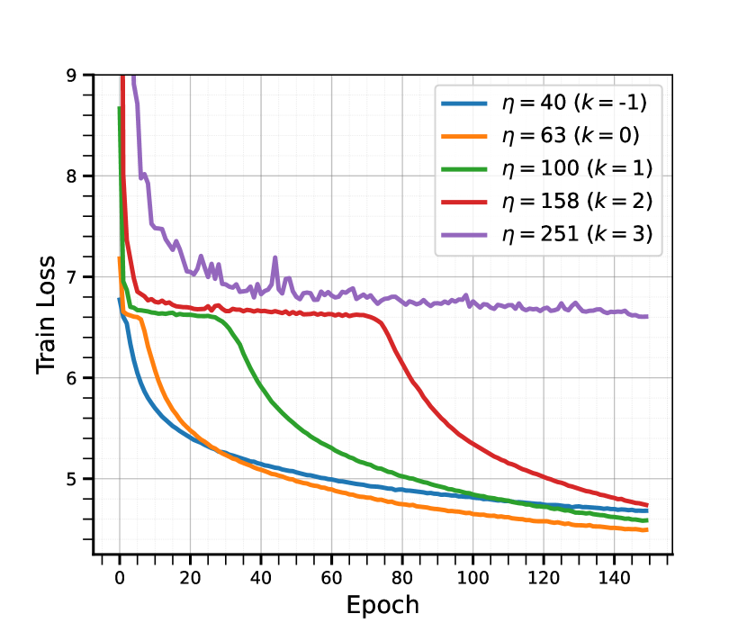
(a) Training curves of NSGD-M.

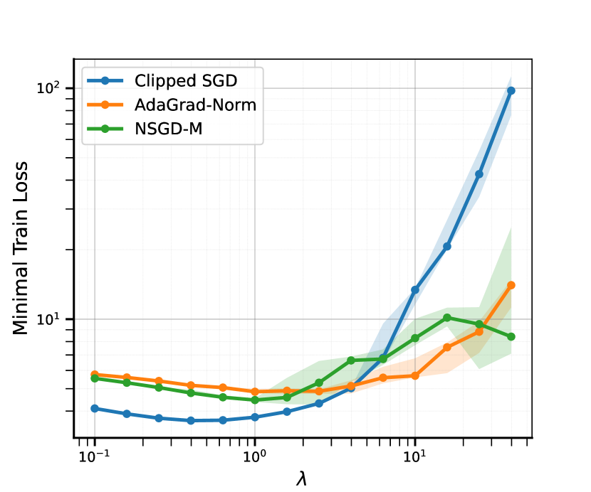
(b) Minimal training loss.

Figure 2: Results on the PTB dataset. Figure 2(a) represents the training curves of NSGD-M for stepsizes $\eta=10^{\nicefrac{{k}}{{5}}}\cdot\eta_{\texttt{opt}}$, where $\eta_{\text{{opt}}}=63$ and $k\in{\left\{-1,0,1,2,3\right\}}$. Figure 2(b) shows the best train loss within $150$ epochs of different algorithms with stepsizes $\lambda\cdot\eta_{\text{{opt}}}$. Shaded areas represent the minimal and maximal value within 5 seeds, the line the median.

Experimental Setup.

To match the assumptions of our theory, we conduct training on the Penn Treebank (PTB) (Mikolov et al.,, 2010) and WikiText-2 (Merity et al.,, 2017) datasets using the AWD-LSTM architecture (Merity et al.,, 2018). Hyperparameters of the model were chosen according to (Merity et al.,, 2018). Besides NSGD-M, we also include AdaGrad-Norm (Faw et al.,, 2023) and Clipped SGD (Zhang et al., 2020b, ). The clipping threshold for Clipped SGD was fixed to be $0.25$ in concordance to previous work (Zhang et al., 2020b, ), the decay-rates of NSGD-M were chosen according to Theorem 2 and $b_{0}$ of AdaGrad-Norm was set to be $b_{0}=10^{-6}$. The code is based on the experiments by Zhang et al., 2020a .

Penn Treebank.

For each algorithm, we select the optimal stepsize $\eta_{\text{{opt}}}$ using a course grid search in a 50 epoch training. The final training was then carried out for $150$ epochs with stepsizes $\eta=\lambda\cdot\eta_{\text{{opt}}}$, where $\lambda=10^{\nicefrac{{k}}{{5}}},k\in{\left\{-5,-4,\dots,8\right\}}$. We replicated this procedure with five seeds for reliable results.

Figure 2(a) shows the behaviour of NSGD-M with different stepsizes. The result supports the narrative behind Theorem 2 that NSGD-M needs an adaption phase before transitioning to a convergence phase. Only after reaching a threshold, NSGD-M starts to decrease the loss. Figure 2(b) focuses on the robustness to hyperparameter selection. It compares the smallest training loss across 150 epochs of different algorithms on scaled versions of their optimally tuned stepsize. As expected, well-tuned Clipped SGD with constant stepsize outperforms all decaying algorithms, while decaying algorithms are more robust to untuned stepsizes. Between NSGD-M and AdaGrad-Norm we notice that NSGD-M has slightly preferable behaviour for small stepsizes. Furthermore the trend for large stepsizes points towards a more robust behaviour of NSGD-M.

WikiText-2.

For each algorithm we first chose the optimal stepsize $\eta_{\text{{opt}}}$ based on a course grid search in a 20 epoch training. The final training was then carried out for $150$ epochs with stepsizes $\eta=\lambda\cdot\eta_{\text{{opt}}}$, where $\lambda=10^{\nicefrac{{k}}{{3}}},k\in{\left\{-3,-4,\dots,5\right\}}$. We replicated this procedure with three seeds for reliable results.

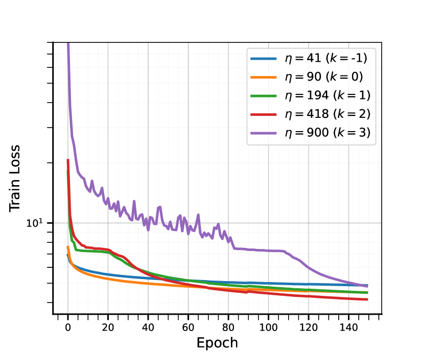
(a) Training curves of NSGD-M.

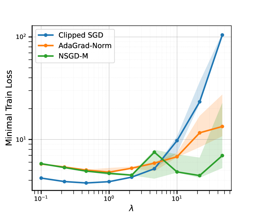
(b) Minimal training loss.

Figure 3: Results on the WikiText-2 dataset. Figure 3(a) represents the logarithmic training curves of NSGD-M for stepsizes $\eta=10^{\nicefrac{{k}}{{3}}}\cdot\eta_{\texttt{opt}}$, where $\eta_{\text{{opt}}}=90$ and $k\in{\left\{-1,0,1,2,3\right\}}$. Figure 3(b) shows the best train loss within $150$ epochs of different algorithms with stepsizes $\lambda\cdot\eta_{\text{{opt}}}$. Shaded areas represent the minimal and maximal value within 3 seeds, the line the median.

In Figure 3(a) we can again notice the same threshold behaviours for NSGD-M as experienced on the PTB dataset. Instead of a plateau we do however observe higher trainings losses before the fast decrease. Training curves of Clipped SGD and AdaGrad-Norm can be found in Figure 4. Figure 3(b) showcases the robustness of NSGD-M to hyperparmeter-tuning to an greater extend than Figure 2(b). We can see that NSGD-M outperforms AdaGrad-Norm for nearly all stepsizes, with the gap increasing as stepsizes increase relative to the optimal stepsize. While Clipped SGD outperforms the adaptive methods when using the optimally-tuned stepsize or less, it suffers from an order of magnitude higher training loss as stepsizes increase relative to the optimally tuned stepsize. When compared to Figure 2(b), a large improvement in performance can be noticed for NSGD-M. We offer the following explanation: While, in both cases, we trained for 150 epochs, the training on the smaller PTB dataset consisted of roughly 680 batches per epoch. On the larger WikiText-2 dataset, epochs consisted of roughly 1500 batches, increasing the total number of iterations from roughly $100000$ to roughly $230000$. When assuming similar values of $L_{0},L_{1}$, NSGD-M hence more likely reached the threshold needed, entering the fast convergence phase, while AdaGrad-Norm behaves more steadily, as can be seen in Figure 4(a).

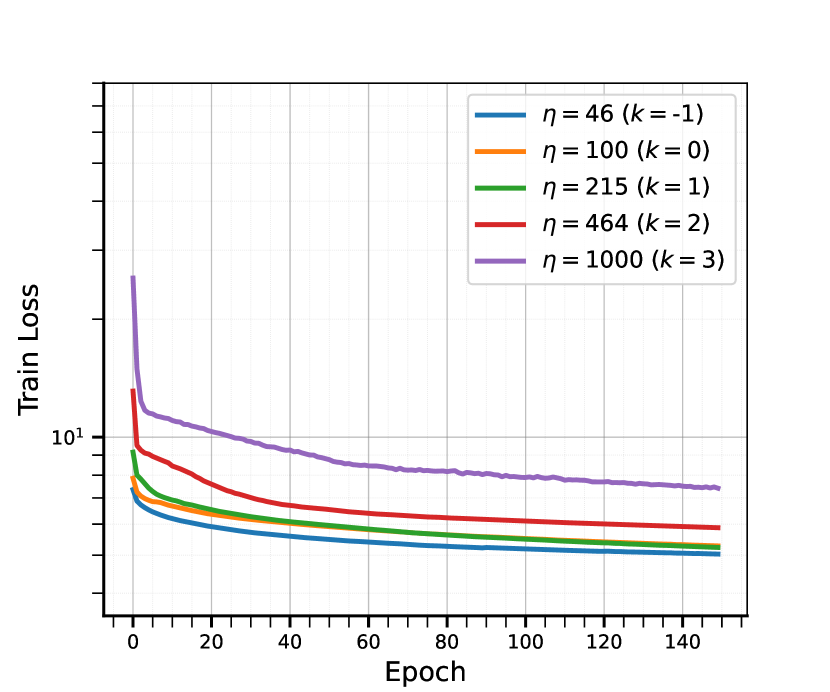
(a) AdaGrad-Norm with $\eta_{\text{{opt}}}=100$.

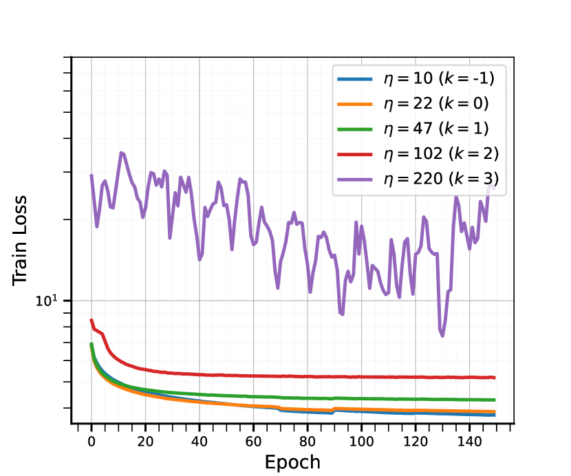
(b) Clipped SGD with $\eta_{\text{{opt}}}=22$.

Figure 4: Logarithmic training curves of AdaGrad-Norm and Clipped SGD on WikiText-2 for stepsizes $\eta=10^{\nicefrac{{k}}{{3}}}\cdot\eta_{\texttt{opt}}$ with $k\in{\left\{-1,0,1,2,3\right\}}$.

6 Conclusion

In this work, we conduct a theoretical investigation into parameter-agnostic algorithms under the ($L_{0},L_{1}$)-smoothness assumption. In the stochastic setting, we show that without requiring any knowledge about problem parameters, Normalized Stochastic Gradient Descent with Momentum (NSGD-M) converges at an order-optimal rate, albeit with an exponential term in $L_{1}$. Further, we introduce a lower bound framework specifically for the parameter-agnostic context, revealing that this exponential term is inescapable for a family of General Normalized Momentum Methods. In the deterministic setting, we show the exponential dependency can be circumvented using GD with Backtracking Line Search while being parameter-agnostic.

This work motivates several questions for future research. The most pressing one is whether there exists a fully parameter-agnostic algorithm in the stochastic setting without an exponential term. Another interesting topic is the derivation of lower bounds for all first-order parameter-agnostic methods.

Appendix A Basic Properties of ($L_{0},L_{1}$)-Smoothness

In this section, we prove basic properties of ($L_{0},L_{1}$)-Smoothness. We start with the proof of the relation to the original definition by Zhang et al., 2020b .

Proof of Lemma 1.

“$\Rightarrow$”: This implication was already shown by Zhang et al., 2020a (, Corollary A.4).

“$\Leftarrow$”: We slightly adapt the proof by Faw et al., (2023, Proposition 1). Assume $F$ is ($L_{0},L_{1}$)-smooth according to Definition 3. Let $x,s\in\mathbb{R}^{d}$ with $\left\lVert s\right\rVert=1$. For $\alpha>0$ our assumption gives

$$\left\lVert{\nabla F}{\left(x+\alpha s\right)}-{{\nabla F}{\left(x\right)}}\right\rVert\leq{\left(A_{0}{\left(\alpha L_{1}\right)}L_{0}+A_{1}{\left(\alpha L_{1}\right)}L_{1}\left\lVert{{\nabla F}{\left(x\right)}}\right\rVert\right)}\alpha,$$

and hence,

$$\left\lVert\frac{{\nabla F}{\left(x+\alpha s\right)}-{{\nabla F}{\left(x\right)}}}{\alpha}\right\rVert\leq A_{0}{\left(\alpha L_{1}\right)}L_{0}+A_{1}{\left(\alpha L_{1}\right)}L_{1}\left\lVert{{\nabla F}{\left(x\right)}}\right\rVert.$$

Using the continuity of norms and the assumption that $F$ is twice continously differentiable, we get

$$L_{0}+L_{1}\left\lVert{{\nabla F}{\left(x\right)}}\right\rVert =\lim_{\alpha\to 0}A_{0}{\left(\alpha L_{1}\right)}L_{0}+A_{1}{\left(\alpha L_{1}\right)}L_{1}\left\lVert{{\nabla F}{\left(x\right)}}\right\rVert$$

$$\geq\lim_{\alpha\to 0}\left\lVert\frac{{\nabla F}{\left(x+\alpha s\right)}-{{\nabla F}{\left(x\right)}}}{\alpha}\right\rVert$$

$$=\left\lVert\lim_{\alpha\to 0}\frac{{\nabla F}{\left(x+\alpha s\right)}-{{\nabla F}{\left(x\right)}}}{\alpha}\right\rVert$$

$$=\left\lVert\nabla^{2}F(x)s\right\rVert.$$

Taking the $\sup$ over all such $s$ yields the claim. ∎

The following lemma serves as the ($L_{0},L_{1}$)-smooth counterpart to the well-known quadratic upper bound on the function value change in the $L$-smooth setting.

Lemma 8 (c.f. (Zhang et al., 2020a, , Lemma A.3)).

Let $d\in\mathbb{N}_{\geq 1}$ and $L_{0},L_{1}\geq 0$. Assume that $f\colon\mathbb{R}^{d}\to\mathbb{R}$ is ($L_{0},L_{1}$)-smooth. Then all $x,y\in\mathbb{R}^{d}$ satisfy

$$f(y)\leq f(x)+{\nabla f}(x)^{\top}(y-x)+\frac{1}{2}{\left(B_{0}{\left(L_{1}\left\lVert x-y\right\rVert\right)}L_{0}+B_{1}{\left(L_{1}\left\lVert x-y\right\rVert\right)}L_{1}\left\lVert{\nabla f}(x)\right\rVert\right)}{\left\lVert x-y\right\rVert^{2}},$$

where

$$B_{0}{\left(c\right)} =1+2\frac{e^{c}-1}{c}-4\frac{e^{c}-1-c}{c^{2}},$$

$$B_{1}{\left(c\right)} =2\frac{e^{c}-1-c}{c^{2}}$$

tend to 1 as $c$ tends towards 0.

Proof.

This proof closely follows the arguments from Zhang et al., 2020a . We include the proof for completeness. Let $x,y\in\mathbb{R}^{d}$ and calculate

$$f(y)-f(x)-{\nabla f}(x)^{\top}(y-x) =\int_{0}^{1}{\nabla f}{\left(x+t(y-x)\right)}^{\top}(y-x)dt-{\nabla f}(x)^{\top}(y-x)$$

$$\leq\int_{0}^{1}\left\lVert{\nabla f}{\left(x+t(y-x)\right)}-{\nabla f}(x)\right\rVert\left\lVert x-y\right\rVert dt$$

$$\leq\left\lVert x-y\right\rVert^{2}{\left(L_{0}\int_{0}^{1}tA_{0}{\left(tc\right)}dt+L_{1}\left\lVert{\nabla f}{\left(x\right)}\right\rVert\int_{0}^{1}tA_{1}{\left(tc\right)}dt\right)}$$

where $c\coloneqq L_{1}\left\lVert x-y\right\rVert$. We now calculate

$$\int_{0}^{1}tA_{0}{\left(tc\right)} =\frac{1}{2}+\frac{e^{c}-1}{c}-2\frac{e^{c}-1-c}{c^{2}}\eqqcolon\frac{1}{2}B_{0}{\left(c\right)}$$

and

$$\int_{0}^{1}A_{1}(tc)dt=\frac{e^{c}-1-c}{c^{2}}\eqqcolon\frac{1}{2}B_{1}{\left(c\right)}.$$

This shows the claim. ∎

Analogous to the $L$-smooth setting, we can also derive an upper bound for the gradient norm based on the suboptimality gap.

Lemma 9 (Gradient Bound, c.f. (Zhang et al., 2020a, , Lemma A.5)).

Let $L_{0},L_{1}>0$ and assume that $f\colon\mathbb{R}^{d}\to\mathbb{R}$ is ($L_{0},L_{1}$)-smooth. Further assume that $f$ is lower bounded by $f^{*}$. Then all $x\in\mathbb{R}^{d}$ satisfy

$$\min{\left\{\frac{\left\lVert{\nabla f}(x)\right\rVert}{L_{1}},\frac{{\left\lVert{\nabla f}(x)\right\rVert^{2}}}{L_{0}}\right\}}\leq 8{\left(f(x)-f^{*}\right)}.$$

Proof.

This proof is again based on Zhang et al., 2020a . We include it since we require parts of the proof later. Let $x\in\mathbb{R}^{d}$. Firstly note that, for $A_{1}$ from Definition 3, the equation

$$c=\frac{L_{1}\left\lVert{\nabla f}(x)\right\rVert}{A_{1}(c)L_{0}+L_{1}A_{1}(c)\left\lVert{\nabla f}(x)\right\rVert}$$

has a solution $c\in(0,1)$. Now we set $\lambda\coloneqq\frac{1}{2A_{1}(c){\left(L_{0}+L_{1}\left\lVert{\nabla f}(x)\right\rVert\right)}}$ and $y\coloneqq x-\lambda{\nabla f}(x)$. Then Lemma 8 yields

$$f^{*}\leq f(y) \leq f(x)-\lambda{\left\lVert{\nabla f}(x)\right\rVert^{2}}+A_{1}{\left(c\right)}{\left(L_{0}+L_{1}\left\lVert{\nabla f}(x)\right\rVert\right)}\lambda^{2}{\left\lVert{\nabla f}(x)\right\rVert^{2}}=f(x)-\frac{\lambda}{2}{\left\lVert{\nabla f}(x)\right\rVert^{2}}.$$

We now differentiate between the two cases $\left\lVert{\nabla f}(x)\right\rVert\leq\frac{L_{0}}{L_{1}}$ and $\left\lVert{\nabla f}(x)\right\rVert>\frac{L_{0}}{L_{1}}$. Therefore,

$$2{\left(f(x)-f^{*}\right)} \geq\frac{{\left\lVert{\nabla f}(x)\right\rVert^{2}}}{A_{1}(c){\left(L_{0}+L_{1}\left\lVert{\nabla f}(x)\right\rVert\right)}}\geq\begin{cases}\frac{{\left\lVert{\nabla f}(x)\right\rVert^{2}}}{4L_{0}},&\text{if}\left\lVert{\nabla f}(x)\right\rVert\leq\frac{L_{0}}{L_{1}}\\ \frac{\left\lVert{\nabla f}(x)\right\rVert}{4L_{1}},&\text{otherwise.}\end{cases}$$

This shows the claim. ∎

Appendix B Technical Lemmas

This section presents crucial technical lemmas and their proofs. These results may be of interest on their own as they can potentially be applied in the analysis of other momentum-based algorithms.

Lemma 10 (Technical Lemma).

Let $q\in(0,1),p\geq 0$ and $t>0$. Further let $a,b\in\mathbb{N}_{\geq 2}$ with $a\leq b$. Then the following statements are true.

• We have

  $$\prod_{t=a}^{b}{\left(1-t^{-q}\right)} \leq\exp{\left(\frac{1}{1-q}{\left(a^{1-q}-b^{1-q}\right)}\right)}.$$

• If $p\geq q$, then

  $$\sum_{t=a}^{b}t^{-p}\prod_{\tau=a}^{t}{\left(1-\tau^{-q}\right)} \leq\frac{{\left(a-1\right)}^{q-p}\exp{\left(\frac{a^{1-q}-{\left(a-1\right)}^{1-q}}{1-q}\right)}-b^{q-p}\exp{\left(\frac{a^{1-q}-b^{1-q}}{1-q}\right)}}{1+{\left(p-q\right)}b^{q-1}},$$

  and in particular,

  $$\sum_{t=a}^{b}t^{-p}\prod_{\tau=a}^{t}{\left(1-\tau^{-q}\right)} \leq{\left(a-1\right)}^{q-p}\exp{\left(\frac{a^{1-q}-{\left(a-1\right)}^{1-q}}{1-q}\right)}=\mathcal{O}{\left(a^{q-p}\right)}.$$

• (c.f. (Fatkhullin et al.,, 2023, Lemma 15)) If $a\geq p^{\frac{1}{1-q}}$ and $a\geq{\left(\frac{p-q}{2}\right)}^{\frac{1}{1-q}}$, then

  $$\sum_{t=a}^{b}t^{-p}\prod_{\tau=t+1}^{b}{\left(1-\tau^{-q}\right)}\leq 2\exp{\left(\frac{1}{1-q}\right)}{\left(b+1\right)}^{q-p}.$$

  Note that these requirements are always fulfilled for $p\leq 1$.

Proof.

$i)$ The first claim follows from the calculation

$$\begin{split}\prod_{t=a}^{b}{\left(1-t^{-q}\right)}&\leq\exp{\left(-\sum_{\tau=a}^{b}t^{-q}\right)}\leq\exp{\left(-\int_{a}^{b+1}t^{-q}dt\right)}=\exp{\left(\frac{1}{{1-q}}{\left(a^{1-q}-{\left(b+1\right)}^{1-q}\right)}\right)},\end{split}$$ (4)

where we used $1-x\leq e^{-x}$ in the first, and the monotonicity of $t^{-q}$ in the second inequality. Weakening the inequality by replacing ${\left(b+1\right)}$ with $b$ finishes the proof.
$ii$) For the second inequality we use $i$) to derive

$$\sum_{t=a}^{b}t^{-p}\prod_{\tau=a}^{t}{\left(1-t^{-q}\right)} \leq\exp{\left(\frac{a^{1-q}}{{1-q}}\right)}\sum_{t=a}^{b}t^{-p}\exp{\left(-\frac{t^{1-q}}{{1-q}}\right)}.$$

Using the monotonicity of $t^{-p}\exp{\left(-t^{1-q}\right)}$ we obtain

$$\sum_{t=a}^{b}t^{-p}\exp{\left(-\frac{t^{1-q}}{{1-q}}\right)} \leq\int_{a-1}^{b}t^{-p}\exp{\left(-\frac{t^{1-q}}{{1-q}}\right)}dt=\int_{a-1}^{b}t^{q-p}t^{-q}\exp{\left(-\frac{t^{1-q}}{{1-q}}\right)}dt.$$

Partial integration now yields

$$\int_{a-1}^{b}t^{q-p}t^{-q}\exp{\left(-\frac{{t}^{1-q}}{{1-q}}\right)}dt$$

$$= \ \left[-t^{q-p}\exp{\left(-\frac{{t}^{1-q}}{{1-q}}\right)}\right]_{t=a-1}^{t=b}-{\left(p-q\right)}\int_{a-1}^{b}t^{{q-p}-1}\exp{\left(-\frac{{t}^{1-q}}{{1-q}}\right)}dt$$

$$= \ {\left(a-1\right)}^{q-p}\exp{\left(-\frac{{{\left(a-1\right)}}^{1-q}}{{1-q}}\right)}-b^{q-p}\exp{\left(-\frac{{b}^{1-q}}{{1-q}}\right)}+{\left({q-p}\right)}\int_{a-1}^{b}t^{{q-p}-1}\exp{\left(-\frac{{t}^{1-q}}{{1-q}}\right)}dt.$$

Finally, we use that $t^{{q-p}-1}\exp{\left(-\frac{{t}^{1-q}}{{1-q}}\right)}$ is monotonically decreasing and $p\geq q$ to derive

$${\left({q-p}\right)}\int_{a-1}^{b}t^{{q-p}-1}\exp{\left(-\frac{{t}^{1-q}}{{1-q}}\right)}dt \leq{\left({q-p}\right)}b^{q-1}\int_{a-1}^{b}t^{-p}\exp{\left(-\frac{{t}^{1-q}}{{1-q}}\right)}dt.$$

Noting that this is the integral we started with and rearranging yields the claim.
$iii$) The proof of the last claim uses the same arguments as in (Fatkhullin et al.,, 2023). First we use $i$) to obtain

$$\sum_{t=a}^{b}t^{-p}\prod_{\tau=t+1}^{b}{\left(1-\tau^{-q}\right)} \leq\sum_{t=a}^{b}t^{-p}\exp{\left(-\sum_{\tau=t+1}^{b}\tau^{-q}\right)}=\exp{\left(-\sum_{\tau=1}^{b}\tau^{-q}\right)}\sum_{t=a}^{b}t^{-p}\exp{\left(\sum_{\tau=1}^{t}\tau^{-q}\right)}.$$

Using the monotonicity of $\tau^{-q}$, we get

$$\exp{\left(-\sum_{\tau=1}^{b}\tau^{-q}\right)}\leq\exp{\left(-\int_{1}^{b+1}\tau^{-q}d\tau\right)}=\exp{\left(\frac{1-{\left(b+1\right)}^{1-q}}{{1-q}}\right)}$$

and

$$\exp{\left(\sum_{\tau=1}^{t}\tau^{-q}\right)}\leq\exp{\left(\int_{0}^{t}\tau^{-q}d\tau\right)}=\exp{\left(\frac{t^{1-q}}{{1-q}}\right)}.$$

We now proceed to bound

$$\sum_{t=a}^{b}t^{-p}\exp{\left(\sum_{\tau=1}^{t}\tau^{-q}\right)}\leq\sum_{t=a}^{b}t^{-p}\exp{\left(\frac{t^{1-q}}{{1-q}}\right)}.$$

Therefore, note that $f{\left(t\right)}\coloneqq t^{-p}\exp{\left(\frac{t^{1-q}}{{1-q}}\right)}$ is monotonically increasing for $t\geq a$ by our assumption on $a$. This implies

$$\sum_{t=a}^{b}t^{-p}\exp{\left(\frac{t^{1-q}}{{1-q}}\right)} \leq\int_{a}^{b+1}t^{-p}\exp{\left(\frac{t^{1-q}}{{1-q}}\right)}dt\eqqcolon I.$$

Integration by party now yields

$$I =\int_{a}^{b+1}t^{q-p}t^{-q}\exp{\left(\frac{t^{1-q}}{{1-q}}\right)}dt$$

$$=\left[t^{q-p}\exp{\left(\frac{{t}^{1-q}}{{1-q}}\right)}\right]_{t=a}^{t=b+1}-{\left({q-p}\right)}\int_{a}^{b+1}t^{{q-p}-1}\exp{\left(\frac{{t}^{1-q}}{{1-q}}\right)}dt$$

$$\leq{\left(b+1\right)}^{q-p}\exp{\left(\frac{{{\left(b+1\right)}}^{1-q}}{{1-q}}\right)}-a^{q-p}\exp{\left(\frac{{a}^{1-q}}{{1-q}}\right)}+{\left(p-q\right)}a^{q-1}I,$$

where we used $p\geq q$ in the last inequality. By our second assumption on $a$ we now get that ${\left(p-q\right)}a^{q-1}\leq\nicefrac{{1}}{{2}}$ and hence

$$I\leq 2{\left(b+1\right)}^{q-p}\exp{\left(\frac{{{\left(b+1\right)}}^{1-q}}{{1-q}}\right)}-2a^{q-p}\exp{\left(\frac{{a}^{1-q}}{{1-q}}\right)}.$$

Putting together the pieces yields

$$\sum_{t=a}^{b}t^{-p}\prod_{\tau=t+1}^{b}{\left(1-\tau^{-q}\right)} \leq 2\exp{\left(\frac{1-{\left(b+1\right)}^{1-q}}{{1-q}}\right)}{\left({\left(b+1\right)}^{q-p}\exp{\left(\frac{{{\left(b+1\right)}}^{1-q}}{{1-q}}\right)}-a^{q-p}\exp{\left(\frac{{a}^{1-q}}{{1-q}}\right)}\right)}$$

$$=2\exp{\left(\frac{1}{{1-q}}\right)}{\left(b+1\right)}^{q-p}-a^{q-p}\exp{\left(\frac{1-{\left(b+1\right)}^{1-q}+a^{1-q}}{{1-q}}\right)},$$

thus proving the last claim. ∎

The following lemma applies the specific values of $p$ and $q$ to Lemma 10.

Lemma 11 (Technical Lemma).

Let $\eta>0$ and for $t\in\mathbb{N}_{\geq 1}$ we set

$${\beta}_{t} \coloneqq 1-t^{-\nicefrac{{1}}{{2}}},$$

$${\eta}_{t} \coloneqq\eta t^{-\nicefrac{{3}}{{4}}}.$$

Then we have

1. For all $T\in\mathbb{N}_{\geq 1}$ the following inequalities hold:

   1. $\sum_{t=1}^{T}{\eta}_{t}\prod_{\tau=2}^{t}{\beta}_{\tau}\leq\frac{7}{2}\eta$;

   2. $\sum_{t=1}^{T}{\eta}_{t}\sqrt{\sum_{\tau=1}^{t}{\alpha}_{\tau}^{2}\prod_{\kappa=\tau+1}^{t}{\beta}_{\kappa}^{2}}\leq\eta{\left(\frac{7}{2}+\sqrt{2e^{2}}\log{\left(T\right)}\right)}.$

2. Let $T\in\mathbb{N}_{\geq 1}$ and define ${C}_{t}\coloneqq 1+2\frac{e^{L_{1}{\eta}_{t}}-1}{L_{1}{\eta}_{t}}-4\frac{e^{L_{1}{\eta}_{t}}-1-L_{1}{\eta}_{t}}{{\left(L_{1}{\eta}_{t}\right)}^{2}}$. Then the following inequalities hold:

   1. $\sum_{t=1}^{T}{\eta}_{t}^{2}{C}_{t}\leq 6\eta^{2}\frac{e^{L_{1}\eta}-1}{L_{1}\eta}$;

   2. $\sum_{t=1}^{T}{\eta}_{t}\sum_{\tau=2}^{t}{\eta}_{\tau}{C}_{\tau}\prod_{\kappa=\tau}^{t}{\beta}_{\kappa}\leq 7\eta^{2}{\left(3\frac{e^{\eta L_{1}}-1}{{\eta L_{1}}}+\log{\left(T\right)}\right)}$.

3. For $t\in\mathbb{N}_{\geq 1}$ we define ${D}_{t}\coloneqq 2\frac{e^{L_{1}{\eta}_{t}}-1-L_{1}{\eta}_{t}}{{\left(L_{1}{\eta}_{t}\right)}^{2}}$ and ${\delta}_{t}\coloneqq 4\eta{\left(t-1\right)}^{\frac{1}{4}}-3\eta.$ Then for all $b\in\mathbb{N}_{\geq 2}$, the following inequalities hold:

   1. $\sum_{t=2}^{b}L_{1}{\eta}_{t}{D}_{t}t^{-{\frac{1}{4}}}{\delta}_{t}e^{L_{1}{\delta}_{t}}\leq\frac{1}{2}\eta^{2}L_{1}e^{2{\eta L_{1}}}+4\eta e^{-\frac{5}{2}{\eta L_{1}}}{\left(e^{4{\eta L_{1}}b^{\frac{1}{4}}}-e^{4{\eta L_{1}}}\right)}$;

   2. $\sum_{t=1}^{b}L_{1}{\eta}_{t}{D}_{t}t^{-{\frac{1}{4}}}e^{L_{1}{\delta}_{t}}\leq\frac{3}{2}{\eta L_{1}}e^{\frac{5}{3}{\eta L_{1}}}+e^{-\frac{5}{2}{\eta L_{1}}}{\left(e^{4{\eta L_{1}}b^{\frac{1}{4}}}-e^{4{\eta L_{1}}}\right)}$;

   3. If additionally ${\eta L_{1}}\geq\frac{1}{2}$, we have $\sum_{t=1}^{b}L_{1}{\eta}_{t}{D}_{t}t^{-{\frac{1}{4}}}e^{L_{1}{\delta}_{t}}\leq\frac{3}{2}{\eta L_{1}}e^{\frac{5}{3}{\eta L_{1}}}+e^{-\frac{5}{2}{\eta L_{1}}}{\left(2b^{-{\frac{1}{4}}}e^{4{\eta L_{1}}b^{\frac{1}{4}}}-e^{4{\eta L_{1}}}\right)}.$

Proof.

Let $T\in\mathbb{N}_{\geq 1}$ and denote $p\coloneqq\nicefrac{{3}}{{4}},q\coloneqq\nicefrac{{1}}{{2}}$ for simplicity.

• The inequality follows from

  $$\sum_{t=1}^{T}{\eta}_{t}\prod_{\tau=2}^{t}{\beta}_{\tau}=\eta+\sum_{t=2}^{T}{\eta}_{t}\prod_{\tau=2}^{t}{\beta}_{\tau}\leq\eta+\eta\exp{\left(2\sqrt{2}-2\right)}\leq\frac{7}{2}\eta,$$

  where we used Lemma 10 $ii$) in the first inequality.

• We start by regrouping

  $$\sum_{t=1}^{T}{\eta}_{t}\sqrt{\sum_{\tau=1}^{t}{\alpha}_{\tau}^{2}\prod_{\kappa=\tau+1}^{t}{\beta}_{\kappa}^{2}} <\sum_{t=1}^{T}{\eta}_{t}{\left(\prod_{\kappa=2}^{t}{\left(1-\kappa^{-q}\right)}+\sqrt{\sum_{\tau=2}^{t}\tau^{-2q}\prod_{\kappa=\tau+1}^{t}{\left(1-\kappa^{-q}\right)}}\right)}.$$

  Applying Lemma 10 $i$), $iii)$ and $a$) $i$) now yields the statement:

  $$\sum_{t=1}^{T}{\eta}_{t}\sqrt{\sum_{\tau=1}^{t}{\alpha}_{\tau}^{2}\prod_{\kappa=\tau+1}^{t}{\beta}_{\kappa}^{2}}\ \ \ {\stackrel{{\scriptstyle\mathclap{i),\ref{lem:technical.general}}}}{{\leq}}}\frac{7}{2}\eta+\sum_{t=2}^{T}{\eta}_{t}\sqrt{2e^{2}{\left(t+1\right)}^{-q}}\leq\eta{\left(\frac{7}{2}+\sqrt{2e^{2}}\log{\left(T\right)}\right)}.$$

  Note that the first inequality is rather loose, a more precise analysis might yield a better result. The above result does however suffice for our use-case.

• First note that

  $${C}_{t}\leq 2\frac{e^{L_{1}{\eta}_{t}}-1}{{L_{1}{\eta}_{t}}}$$ (5)

  and hence

  $$\sum_{t=1}^{T}{\eta}_{t}^{2}{C}_{t}\leq\frac{2}{L_{1}}\sum_{t=1}^{T}{\eta}_{t}{\left(e^{L_{1}{\eta}_{t}}-1\right)}.$$ (6)

  Now we calculate

  $$\begin{split}\sum_{t=1}^{T}{\eta}_{t}{\left(e^{L_{1}{\eta}_{t}}-1\right)}&\leq\eta^{2}\frac{e^{\eta L_{1}}-1}{\eta}+\int_{1}^{T}{\eta}_{t}{\left(e^{L_{1}{\eta}_{t}}-1\right)}dt=\eta^{2}{\left(\frac{e^{\eta L_{1}}-1}{\eta}+\frac{1}{\eta}\int_{1}^{T}t^{-p}{\left(e^{L_{1}{\eta}_{t}}-1\right)}\right)}\end{split}$$ (7)

  and further

  $$\int_{1}^{T}t^{-p}{\left(e^{L_{1}{\eta}_{t}}-1\right)} =\int_{1}^{T}t^{-p}\sum_{k=1}^{\infty}\frac{{\left({\eta L_{1}}t^{-p}\right)}^{k}}{k!}dt=\sum_{k=1}^{\infty}\int_{1}^{T}\frac{{\left({\eta L_{1}}\right)}^{k}}{k!}t^{-p(k+1)}dt,$$ (8)

  where we used that the exponential series converges locally uniformly in the second equality. Finally we calculate for $k\geq 2$

  $$\int_{1}^{T}t^{-p{\left(k+1\right)}}dt =\frac{4}{-3k+1}{\left(T^{-p{\left(k+1\right)}+1}-1\right)}\leq\frac{4}{3k-1}\leq\frac{4}{k+1}.$$ (9)

  Combining (8) and (9) now yields

  $$\int_{1}^{T}t^{-p}{\left(e^{L_{1}{\eta}_{t}}-1\right)} \leq 4\sum_{k=1}^{\infty}\frac{{\left({\eta L_{1}}\right)}^{k}}{{\left(k+1\right)}!}=4\frac{e^{\eta L_{1}}-1-{\eta L_{1}}}{{\eta L_{1}}}$$ (10)

  and hence

  $$\sum_{t=1}^{T}{\eta}_{t}^{2}{C}_{t}\stackrel{{\scriptstyle\mathclap{\eqref{lzlo.infnsgd.eq:explicit_technical_bounds_bi_1}}}}{{\leq}} \frac{2}{L_{1}}\sum_{t=1}^{T}{\eta}_{t}{\left(e^{L_{1}{\eta}_{t}}-1\right)}$$

  $$\stackrel{{\scriptstyle\mathclap{\eqref{lzlo.infnsgd.eq:explicit_technical_bounds_bi_2}}}}{{\leq}} \eta^{2}{\left(2\frac{e^{\eta L_{1}}-1}{{\eta L_{1}}}+\frac{2}{{\eta L_{1}}}\int_{1}^{T}t^{-p}{\left(e^{L_{1}{\eta}_{t}}-1\right)}dt\right)}$$

  $$\stackrel{{\scriptstyle\mathclap{\eqref{lzlo.infnsgd.eq:explicit_technical_bounds_bi_5}}}}{{\leq}} \eta^{2}{\left(2\frac{e^{\eta L_{1}}-1}{{\eta L_{1}}}+8\frac{e^{\eta L_{1}}-1-{\eta L_{1}}}{{\left({\eta L_{1}}\right)}^{2}}\right)}.$$

  The claim now follows by noting that for all $x\geq 0$ the inequality $2\frac{e^{x}-1-x}{x^{2}}\leq\frac{e^{x}-1}{x}$ is satisfied.

• Firstly, $a$) $i$) yields

  $$\sum_{t=1}^{T}\sum_{\tau=2}^{t}{\eta}_{t}{\eta}_{\tau}{\left(\prod_{\kappa=\tau}^{t}{\beta}_{\kappa}\right)}{C}_{\tau} =\sum_{\tau=2}^{T}{\eta}_{\tau}{C}_{\tau}\sum_{t=\tau}^{T}{\eta}_{t}\prod_{\kappa=\tau}^{t}{\beta}_{\kappa}\stackrel{{\scriptstyle a)i)}}{{\leq}}\frac{7}{2}\eta\sum_{\tau=2}^{T}{\eta}_{\tau}{C}_{\tau}{\left(\tau-1\right)}^{q-p}\leq\frac{7}{2}\eta^{2}\sum_{\tau=1}^{T}\tau^{-1}{C}_{\tau}.$$ (11)

  To upper bound $\sum_{t=1}^{T}t^{-1}{C}_{t}$ we first use (5) to get

  $$\sum_{t=1}^{T}t^{-1}{C}_{t}\stackrel{{\scriptstyle\eqref{lzlo.infnsgd.eq:explicit_technical_bounds_Ct_bound}}}{{\leq}}2\sum_{t=1}^{T}t^{-1}\frac{e^{L_{1}{\eta}_{t}}-1}{{L_{1}{\eta}_{t}}}\leq 2\frac{e^{\eta L_{1}}-1}{{\eta L_{1}}}+2\sum_{t=2}^{T}t^{-1}\frac{e^{L_{1}{\eta}_{t}}-1}{{L_{1}{\eta}_{t}}}.$$

  Next we focus on bounding $\sum_{t=2}^{T}t^{-1}\frac{e^{L_{1}{\eta}_{t}}-1}{{L_{1}{\eta}_{t}}}$. We therefore again use the locally uniform convergence of the exponential series to get

  $$\sum_{t=2}^{T}t^{-1}\frac{e^{L_{1}{\eta}_{t}}-1}{{L_{1}{\eta}_{t}}} \leq\int_{1}^{T}t^{-1}\sum_{k=1}^{\infty}\frac{{\left({L_{1}{\eta}_{t}}\right)}^{k-1}}{k!}dt$$

  $$=\frac{1}{{\eta L_{1}}}\sum_{k=1}^{\infty}\frac{{\left({\eta L_{1}}\right)}^{k}}{k!}\int_{1}^{T}t^{-pk-\nicefrac{{1}}{{4}}}dt$$

  $$=\log{\left(T\right)}+\frac{1}{{\left({\eta L_{1}}\right)}^{2}}\sum_{k=2}^{\infty}\frac{{\left({\eta L_{1}}\right)}^{k+1}}{k!}\frac{1-T^{-p{\left(k-1\right)}}}{p{\left(k-1\right)}}$$

  $$\leq\log{\left(T\right)}+\frac{4}{{\left({\eta L_{1}}\right)}^{2}}\sum_{k=2}^{\infty}\frac{{\left({\eta L_{1}}\right)}^{k+1}}{{\left(k+1\right)}!},$$

  where we used that $3(k-1)\geq k+1$ for $k\geq 2$. Putting the above together and using that $2\frac{e^{x}-1-x-x^{2}/2}{x^{2}}\leq\frac{e^{x}-1}{x}$ for $x\geq 0$ gives

  $$\sum_{t=1}^{T}\sum_{\tau=2}^{t}{\eta}_{t}{\eta}_{\tau}{\left(\prod_{\kappa=\tau}^{t}{\beta}_{\kappa}\right)}{C}_{\tau}\leq\frac{7}{2}\eta^{2}{\left(2\frac{e^{\eta L_{1}}-1}{{\eta L_{1}}}+2\log{\left(T\right)}+4\frac{e^{\eta L_{1}}-1}{{\eta L_{1}}}\right)}=7\eta^{2}{\left(\log{\left(T\right)}+3\frac{e^{\eta L_{1}}-1}{{\eta L_{1}}}\right)}$$

  and hence proves the claim.

• We start off by calculating

  $$\sum_{t=2}^{b}L_{1}{\eta}_{t}{D}_{t}t^{-{\frac{1}{4}}}{\delta}_{t}e^{L_{1}{\delta}_{t}} \leq L_{1}{\eta}_{2}{D}_{2}2^{-{\frac{1}{4}}}\eta e^{\eta L_{1}}+\sum_{t=3}^{b}L_{1}{\eta}_{t}{D}_{t}t^{-{\frac{1}{4}}}{\delta}_{t}e^{L_{1}{\delta}_{t}}$$

  $$\leq\frac{1}{2}\eta^{2}L_{1}e^{2{\eta L_{1}}}+4\eta\sum_{t=3}^{b}L_{1}{\eta}_{t}{D}_{t}e^{L_{1}{\delta}_{t}}$$

  and further

  $$\begin{split}\sum_{t=3}^{b}L_{1}{\eta}_{t}{D}_{t}e^{L_{1}{\delta}_{t}}&\leq\sum_{t=3}^{b}L_{1}{\eta}_{t}\exp{\left(L_{1}{\left(4\eta{\left(t-1\right)}^{\frac{1}{4}}-3\eta+{\eta}_{t}\right)}\right)}\\ &\leq e^{-\frac{5}{2}{\eta L_{1}}}\sum_{t=3}^{b}L_{1}{\eta}_{t-1}e^{4{\eta L_{1}}{\left(t-1\right)}^{\frac{1}{4}}}\\ &\leq e^{-\frac{5}{2}{\eta L_{1}}}\int_{2}^{b+1}{\eta L_{1}}{\left(t-1\right)}^{-p}e^{4{\eta L_{1}}{\left(t-1\right)}^{1-p}}dt\\ &=e^{-\frac{5}{2}{\eta L_{1}}}{\left(e^{4{\eta L_{1}}b^{\frac{1}{4}}}-e^{4{\eta L_{1}}}\right)}.\end{split}$$ (12)

  Here we used that $g{\left(t\right)}\coloneqq L_{1}{\eta}_{{t-1}}e^{4\eta L_{1}{\left(t-1\right)}^{\frac{1}{4}}}$ is non-negative and monotonically decreasing before turning monotonically increasing in the third inequality. Noting that (12) also holds for $b=2$ yields the claim.

• We have

  $$\begin{split}\sum_{t=1}^{b}L_{1}{\eta}_{t}{D}_{t}t^{-{\frac{1}{4}}}e^{L_{1}{\delta}_{t}}&={\eta L_{1}}{D}_{1}+\frac{1}{2}{\eta L_{1}}{D}_{2}e^{\eta L_{1}}+\sum_{t=3}^{b}L_{1}{\eta}_{t}{D}_{t}t^{-{\frac{1}{4}}}e^{L_{1}{\delta}_{t}}\\ &\leq{\eta L_{1}}e^{\eta L_{1}}+\frac{1}{2}{\eta L_{1}}e^{{\left(1+2^{-\frac{3}{4}}\right)}{\eta L_{1}}}+\sum_{t=3}^{b}{L_{1}{\eta}_{t}}{D}_{t}e^{L_{1}{\delta}_{t}}\end{split}$$ (13)

  and using (12) yields

  $$\sum_{t=1}^{b}L_{1}{\eta}_{t}{D}_{t}t^{-{\frac{1}{4}}}e^{L_{1}{\delta}_{t}} \leq\frac{3}{2}{\eta L_{1}}e^{\frac{5}{3}{\eta L_{1}}}+e^{-\frac{5}{2}{\eta L_{1}}}{\left(e^{4{\eta L_{1}}b^{\frac{1}{4}}}-e^{4{\eta L_{1}}}\right)}.$$

• We first again calculate

  $$\sum_{t=3}^{b}L_{1}{\eta}_{t}{D}_{t}t^{-{\frac{1}{4}}}e^{L_{1}{\delta}_{t}} \leq e^{-\frac{5}{2}{\eta L_{1}}}\int_{2}^{b+1}t^{-{\frac{1}{4}}}L_{1}\eta{\left(t-1\right)}^{-\frac{3}{4}}e^{4{\eta L_{1}}{\left(t-1\right)}^{\frac{1}{4}}}dt$$

  before, similar to the proof of Lemma 10 $iii$), using partial integration to derive

  $$I \coloneqq\int_{2}^{b+1}t^{-{\frac{1}{4}}}L_{1}\eta{\left(t-1\right)}^{-\frac{3}{4}}e^{4{\eta L_{1}}{\left(t-1\right)}^{\frac{1}{4}}}dt$$

  $$=\left[t^{-{\frac{1}{4}}}e^{4{\eta L_{1}}{\left(b-1\right)}^{\frac{1}{4}}}\right]_{t=2}^{t=b+1}+{\frac{1}{4}}\int_{2}^{b+1}t^{-\frac{5}{4}}e^{4{\eta L_{1}}{\left(t-1\right)}^{\frac{1}{4}}}dt$$

  $$\leq b^{-{\frac{1}{4}}}e^{4{\eta L_{1}}b^{\frac{1}{4}}}-\frac{1}{2}e^{4{\eta L_{1}}}+\frac{1}{2^{\frac{1}{4}}4{\eta L_{1}}}\int_{2}^{b+1}{\eta L_{1}}{\left(t-1\right)}^{-1}e^{4{\eta L_{1}}{\left(t-1\right)}^{\frac{1}{4}}}$$

  $$\leq b^{-{\frac{1}{4}}}e^{4{\eta L_{1}}b^{\frac{1}{4}}}-\frac{1}{2}e^{4{\eta L_{1}}}+\frac{1}{4{\eta L_{1}}}I.$$

  By our assumption we have $\frac{1}{4{\eta L_{1}}}\leq\frac{1}{2}$ and hence

  $$I\leq 2b^{-{\frac{1}{4}}}e^{4{\eta L_{1}}b^{\frac{1}{4}}}-e^{4{\eta L_{1}}}.$$

  Finally (13) yields the claim.

∎

Appendix C Missing Proofs

This section contains the proofs for Section 3 and Section 4.

C.1 Proofs for Parameter-Agnostic Upper Bounds

C.1.1 Stochastic Setting

We start with the proof of Theorem 2, which has the same structure as in the $L$-smooth setting (Cutkosky and Mehta,, 2020): We first derive a Descent Lemma, second bound the momentum deviation $\left\lVert{m}_{t}-{\nabla F}{\left({x}_{t}\right)}\right\rVert$ and third combine these two to show the result. The last step is however more intricate, as large stepsizes in the beginning can lead to an exponential increase in the gradient norm. The main intuitions behind the third step are the following:

Due to potentially too large stepsizes, we cannot use the descent lemma to control the expected gradient norm in the beginning. Only after reaching a threshold $t_{0}\propto{\left({\eta L_{1}}\right)}^{4}$ the gradient norms can be controlled in this fashion. Before this threshold, in the adaption phase, we instead use ($L_{0},L_{1}$)-smoothness to control the gradient norms based on $\left\lVert{\nabla F}{\left({{x}_{1}}\right)}\right\rVert$. After this threshold, in the convergence phase, Lemma 11 essentially establishes that the diminishing step-size rule ${\eta}_{t}=t^{-p}$ exhibits the same asymptotically behaviour as if the stepsizes were chosen constantly as ${\eta}_{t}\equiv T^{-p}$, where $T$ denotes the iteration horizon. This aligns with the behaviour of NSGD-M in the $L$-smooth setting (Yang et al.,, 2022). In particular, this implies that $p=\nicefrac{{3}}{{4}}$ is the only possible choice to achieve the optimal complexity (Cutkosky and Mehta,, 2020; Zhang et al., 2020a, ).

Unless stated otherwise, the notations ${\left\{{\xi}_{1},{\xi}_{2},\dots\right\}},{\left\{{g}_{1},{g}_{2},\dots\right\}},{\left\{{m}_{1},{m}_{2},\dots\right\}}$ and ${\left\{{x}_{1},{x}_{2},\dots\right\}}$ correspond to the iterations generated by NSGD-M throughout this section. We denote the natural filtration of ${{\xi}_{1},\dots,{\xi}_{t}}$ with respect to the underlying probability space by ${\mathcal{F}}_{t}\coloneqq\sigma{\left({{\xi}_{1},{\xi}_{2},\dots,{\xi}_{t}}\right)}$.

Lemma 12 (Descent Lemma).

Assume ( (($L_{0},L_{1}$)-smoothness).) and let $t\in\mathbb{N}_{\geq 2}$. Then

$$F{\left({x}_{{t+1}}\right)}-F{\left({x}_{t}\right)}\leq-{\eta}_{t}\left\lVert{\nabla F}{\left({x}_{t}\right)}\right\rVert+2{\eta}_{t}\left\lVert{\nabla F}{\left({x}_{t}\right)}-{m}_{t}\right\rVert+\frac{{\eta}_{t}^{2}}{2}{\left(L_{0}{C}_{t}+L_{1}{D}_{t}\left\lVert{\nabla F}{\left({x}_{t}\right)}\right\rVert\right)},$$

where ${C}_{t}\coloneqq B_{0}{\left(L_{1}{\eta}_{t}\right)}$ and ${D}_{t}\coloneqq B_{1}{\left(L_{1}{\eta}_{t}\right)}$, where $B_{0},B_{1}$ are as defined in Lemma 8. If we further assume ( (Lower Boundedness).) we also get

$$\sum_{t=1}^{T}{\left({\eta}_{t}-\frac{L_{1}{\eta}_{t}^{2}{D}_{t}}{2}\right)}\left\lVert{\nabla F}{\left({x}_{t}\right)}\right\rVert \leq\Delta_{1}+\frac{L_{0}}{2}\sum_{t=1}^{T}{\eta}_{t}^{2}{C}_{t}+2\sum_{t=1}^{T}{\eta}_{t}\left\lVert{\nabla F}{\left({x}_{t}\right)}-{m}_{t}\right\rVert,$$

where $\Delta_{1}\coloneqq F{\left({{x}_{1}}\right)}-F^{*}$.

Proof.

The proof follows the arguments by Zhao et al., (2021). Using Lemma 8 we get

$$F{\left({x}_{{t+1}}\right)}-F{\left({x}_{t}\right)} \leq{\nabla F}{\left({x}_{t}\right)}^{\top}{\left({x}_{{t+1}}-{x}_{t}\right)}+\frac{{\eta}_{t}^{2}}{2}{\left(L_{0}{C}_{t}+L_{1}{D}_{t}\left\lVert{\nabla F}{\left({x}_{t}\right)}\right\rVert\right)}$$

$$=-\frac{{\eta}_{t}}{\left\lVert{m}_{t}\right\rVert}{\nabla F}(x)^{\top}{m}_{t}+\frac{{\eta}_{t}^{2}}{2}{\left(L_{0}{C}_{t}+L_{1}{D}_{t}\left\lVert{\nabla F}{\left({x}_{t}\right)}\right\rVert\right)}$$

$$=-\frac{{\eta}_{t}}{\left\lVert{m}_{t}\right\rVert}{\left({\nabla F}{\left({x}_{t}\right)}-{m}_{t}\right)}^{\top}{m}_{t}-{\eta}_{t}\left\lVert{m}_{t}\right\rVert+\frac{{\eta}_{t}^{2}}{2}{\left(L_{0}{C}_{t}+L_{1}{D}_{t}\left\lVert{\nabla F}{\left({x}_{t}\right)}\right\rVert\right)}.$$

Utilizing Cauchy-Schwarz and ${\eta}_{t}\left\lVert{\nabla F}{\left({x}_{t}\right)}\right\rVert\leq{\eta}_{t}\left\lVert{\nabla F}{\left({x}_{t}\right)}-{m}_{t}\right\rVert+{\eta}_{t}\left\lVert{m}_{t}\right\rVert$ now yields

$$F{\left({x}_{{t+1}}\right)}-F{\left({x}_{t}\right)} \leq-{\eta}_{t}\left\lVert{\nabla F}{\left({x}_{t}\right)}\right\rVert+2\left\lVert{\nabla F}{\left({x}_{t}\right)}-{m}_{t}\right\rVert+\frac{{\eta}_{t}^{2}}{2}{\left(L_{0}{C}_{t}+L_{1}{D}_{t}\left\lVert{\nabla F}{\left({x}_{t}\right)}\right\rVert\right)}$$

and hence the first claim. For the second statement we sum up to get

$$\sum_{t=1}^{T}{\left({\eta}_{t}-\frac{L_{1}{\eta}_{t}^{2}{D}_{t}}{2}\right)}\left\lVert{\nabla F}{\left(x\right)}\right\rVert\leq\Delta_{1}+\frac{1}{2}\sum_{t=1}^{T}L_{0}{\eta}_{t}^{2}{C}_{t}+2\sum_{t=1}^{T}{\eta}_{t}\left\lVert{\nabla F}{\left({x}_{t}\right)}-{m}_{t}\right\rVert.$$

∎

Lemma 13 (General Momentum Deviation Bound).

Assume ( (($L_{0},L_{1}$)-smoothness).), ( (Bounded Variance).) and let $t\in\mathbb{N}_{\geq 1}$. Suppose ${\beta}_{1}=0$. Then we have

$$\mathbb{E}\left[\left\lVert{m}_{t}-{\nabla F}{\left({x}_{t}\right)}\right\rVert\right]\leq \ \sigma\sqrt{\sum_{\tau=1}^{t}\beta_{{\left(\tau+1\right)}:t}^{2}{\left(1-{\beta}_{\tau}\right)}^{2}}+L_{0}\sum_{\tau=2}^{t}{\eta}_{\tau}\beta_{\tau:t}{C}_{\tau}+L_{1}\sum_{\tau=2}^{t}{\eta}_{\tau}\beta_{\tau:t}{D}_{\tau}\mathbb{E}\left[\left\lVert{\nabla F}{\left({x}_{\tau}\right)}\right\rVert\right],$$

where $\beta_{a:b}$ denotes $\prod_{t=a}^{b}{\beta}_{t}$ and ${C}_{t},{D}_{t}$ are defined as in Lemma 12.

Proof.

This proof is motivated by Cutkosky and Mehta, (2020), and similar arguments are carried by Zhang et al., 2020a and Yang et al., (2022). To simplify notation we first define

$${\mu}_{t} \coloneqq{m}_{t}-{\nabla F}{\left({x}_{t}\right)},$$

$${\gamma}_{t} \coloneqq{g}_{t}-{\nabla F}{\left({x}_{t}\right)},$$

$${\alpha}_{t} \coloneqq 1-{\beta}_{t},$$

$$\beta_{a:b} \coloneqq\prod_{t=a}^{b}{\beta}_{t}.$$

Now let $i,j\in\mathbb{N},i<j$ and calculate

$$\begin{split}\mathbb{E}\left[{\gamma}_{j}^{\top}{\gamma}_{i}\right]&=\mathbb{E}\left[\mathbb{E}\left[{\gamma}_{j}^{\top}{\gamma}_{i}\,\middle|\,\mathcal{F}_{j-1}\right]\right]\\ &=\mathbb{E}\left[\mathbb{E}\left[{\gamma}_{j}\,\middle|\,\mathcal{F}_{j-1}\right]^{\top}{\gamma}_{i}\right]\\ &=0,\end{split}$$ (14)

where we used that $\mathbb{E}\left[{\gamma}_{j}\,\middle|\,\mathcal{F}_{j-1}\right]=0$ in the last equality. Next we define ${S}_{t}\coloneqq{\nabla F}{\left({x}_{{t-1}}\right)}-{\nabla F}{\left({x}_{t}\right)}$ and calculate

$${m}_{t} ={\beta}_{t}{m}_{{t-1}}+{\left(1-{\beta}_{t}\right)}{g}_{t}$$

$$={\beta}_{t}{\left({\nabla F}{\left({x}_{{t-1}}\right)}+{\mu}_{{t-1}}\right)}+{\left(1-{\beta}_{t}\right)}{\left({\gamma}_{t}+{\nabla F}{\left({x}_{t}\right)}\right)}$$

$$={\nabla F}{\left({x}_{t}\right)}+{\left(1-{\beta}_{t}\right)}{\gamma}_{t}+{\beta}_{t}{S}_{t}+{\beta}_{t}{\mu}_{{t-1}}.$$

This yields

$${\mu}_{t} =\beta_{2:t}{\mu}_{1}+\sum_{\tau=2}^{t}\beta_{{\left(\tau+1\right)}:t}{\alpha}_{\tau}{\gamma}_{\tau}+\sum_{\tau=2}^{t}\beta_{\tau:t}{S}_{\tau}=\sum_{\tau=1}^{t}\beta_{{\left(\tau+1\right)}:t}{\alpha}_{\tau}{\gamma}_{\tau}+\sum_{\tau=2}^{t}\beta_{\tau:t}{S}_{\tau},$$

where we used ${\beta}_{1}=0$ in the second inequality. Therefore

$$\mathbb{E}\left[\left\lVert{\mu}_{t}\right\rVert\right] \leq\mathbb{E}\left[\left\lVert\sum_{\tau=1}^{t}\beta_{{\left(\tau+1\right)}:t}{\alpha}_{\tau}{\gamma}_{\tau}\right\rVert\right]+\sum_{\tau=2}^{t}\beta_{\tau:t}\mathbb{E}\left[\left\lVert{S}_{\tau}\right\rVert\right].$$

To further concretize this upper bound, (14) firstly yields

$$\mathbb{E}\left[\left\lVert\sum_{\tau=1}^{t}\beta_{{\left(\tau+1\right)}:t}{\alpha}_{\tau}{\gamma}_{\tau}\right\rVert\right] \leq\sqrt{\sum_{\tau=1}^{t}\beta_{{\left(\tau+1\right)}:t}^{2}{\alpha}_{t}^{2}\sigma^{2}}.$$

Secondly, ( (($L_{0},L_{1}$)-smoothness).) implies

$$\left\lVert{S}_{t}\right\rVert \leq{\eta}_{t}{\left({C}_{t}L_{0}+{D}_{t}L_{1}\left\lVert{\nabla F}{\left({x}_{t}\right)}\right\rVert\right)}$$

and hence

$$\sum_{\tau=2}^{t}\beta_{\tau:t}\mathbb{E}\left[\left\lVert{S}_{\tau}\right\rVert\right] \leq L_{0}\sum_{\tau=2}^{t}{\eta}_{\tau}\beta_{\tau:t}{C}_{\tau}+L_{1}\sum_{\tau=2}^{t}{\eta}_{\tau}\beta_{\tau:t}{D}_{\tau}\mathbb{E}\left[\left\lVert{\nabla F}{\left({x}_{\tau}\right)}\right\rVert\right].$$

Putting these results together we get the claim. ∎

Now we are ready for the main result.

Theorem 14 (NSGD-M for ($L_{0},L_{1}$)-smoothness).

Assume ( (Lower Boundedness).), ( (($L_{0},L_{1}$)-smoothness).) and ( (Bounded Variance).). Let $\eta>0$ and define the parameters

$${\beta}_{t} \coloneqq 1-t^{-\nicefrac{{1}}{{2}}}$$

$${\eta}_{t} \coloneqq\eta t^{-\nicefrac{{3}}{{4}}}.$$

Then NSGD-M with starting point ${x}_{1}\in\mathbb{R}^{d}$ satisfies

$$\sum_{t=1}^{T}\frac{{\eta}_{t}}{2}\mathbb{E}\left[\left\lVert{\nabla F}{\left({x}_{t}\right)}\right\rVert\right]\leq \ \Delta_{1}+\eta\sigma{\left(7+2\sqrt{2e^{2}}\log{\left(T\right)}\right)}+\eta^{2}L_{0}{\left(45\frac{e^{\eta L_{1}}-1}{{\eta L_{1}}}+14\log{\left(T\right)}\right)}$$

$$\ +21\eta^{2}L_{0}e^{48{\left({\eta L_{1}}\right)}^{2}}+6\eta e^{48{\left({\eta L_{1}}\right)}^{2}}\left\lVert{\nabla F}{\left({{x}_{1}}\right)}\right\rVert,$$

where $\Delta_{1}\coloneqq F{\left({{x}_{1}}\right)}-F^{*}$. Furthermore, if $L_{1}\geq\nicefrac{{1}}{{2\eta}}$, the statement also holds when replacing $6\eta e^{48{\left({\eta L_{1}}\right)}^{2}}\left\lVert{\nabla F}{\left({{x}_{1}}\right)}\right\rVert$ with $\frac{e^{48{\left({\eta L_{1}}\right)}^{2}}}{L_{1}}\left\lVert{\nabla F}{\left({{x}_{1}}\right)}\right\rVert$.

The main workhorse behind the following proof is Lemma 11. It intuitively states that the quantities which emerge due to the nonconstant parameters behave (nearly) asymptotically the same as constant stepsizes would.

Proof.

To simplify notation we define

$$\beta_{a:b}\coloneqq\prod_{\tau=a}^{b}{\beta}_{\tau}.$$

We start the proof by combining Lemma 12 and Lemma 13 to obtain

$$\sum_{t=1}^{T}{\eta}_{t}\mathbb{E}\left[\left\lVert{\nabla F}{\left({x}_{t}\right)}\right\rVert\right]\stackrel{{\scriptstyle\mathclap{\ref{lem:analysis.descent_lemma}}}}{{\leq}} \,\Delta_{1}+\frac{L_{0}}{2}\sum_{t=1}^{T}{\eta}_{t}^{2}{C}_{t}+\frac{L_{1}}{2}\sum_{t=1}^{T}{\eta}_{t}^{2}{D}_{t}\mathbb{E}\left[\left\lVert{\nabla F}{\left({x}_{t}\right)}\right\rVert\right]+2\sum_{t=1}^{T}{\eta}_{t}\mathbb{E}\left[\left\lVert{\nabla F}{\left({x}_{t}\right)}-{m}_{t}\right\rVert\right]$$

$$\stackrel{{\scriptstyle\mathclap{\ref{lem:analysis.mu_bound}}}}{{\leq}} \,\Delta_{1}+\frac{L_{0}}{2}\sum_{t=1}^{T}{\eta}_{t}^{2}{C}_{t}+\frac{L_{1}}{2}\sum_{t=1}^{T}{\eta}_{t}^{2}{D}_{t}\mathbb{E}\left[\left\lVert{\nabla F}{\left({x}_{t}\right)}\right\rVert\right]+2\sigma\sum_{t=1}^{T}{\eta}_{t}\sqrt{\sum_{\tau=1}^{t}{\alpha}_{\tau}^{2}{\left(\beta_{{\left(\tau+1\right)}:t}\right)}^{2}}$$

$$\ +2L_{0}\sum_{t=1}^{T}{\eta}_{t}\sum_{\tau=2}^{t}{\eta}_{\tau}{C}_{\tau}\beta_{\tau:t}+2L_{1}\sum_{t=1}^{T}{\eta}_{t}\sum_{\tau=2}^{t}{\eta}_{\tau}{D}_{\tau}\beta_{\tau:t}\mathbb{E}\left[\left\lVert{\nabla F}{\left({x}_{\tau}\right)}\right\rVert\right].$$

Next, we use Lemma 11 $a$) and $b$) to bound all terms that are independent of the iterates ${x}_{t}$. This leaves us with

$$\begin{split}\sum_{t=1}^{T}{\eta}_{t}\mathbb{E}\left[\left\lVert{\nabla F}{\left({x}_{t}\right)}\right\rVert\right]\leq&\ \Delta_{1}+\eta\sigma{\left(7+2\sqrt{2e^{2}}\log{\left(T\right)}\right)}+\eta^{2}L_{0}{\left(45\frac{e^{\eta L_{1}}-1}{{\eta L_{1}}}+14\log{\left(T\right)}\right)}\\ &\ +\underbrace{\frac{L_{1}}{2}\sum_{t=1}^{T}{\eta}_{t}^{2}{D}_{t}\mathbb{E}\left[\left\lVert{\nabla F}{\left({x}_{t}\right)}\right\rVert\right]+2L_{1}\sum_{\tau=2}^{T}{\eta}_{\tau}{\left(\sum_{t=\tau}^{T}{\eta}_{t}\beta_{\tau:t}\right)}{D}_{\tau}\mathbb{E}\left[\left\lVert{\nabla F}{\left({x}_{\tau}\right)}\right\rVert\right]}_{\eqqcolon(A)},\end{split}$$ (15)

where we rearranged the sums of the last term. We then focus on upper bounding $(A)$. Therefore we use Lemma 10 $ii)$ which yields

$$(A) \leq\sum_{t=1}^{T}{\eta}_{t}{D}_{t}{\left(\frac{L_{1}}{2}{\eta}_{t}+2e^{2{\left(\sqrt{2}-1\right)}}L_{1}\eta t^{-{\frac{1}{4}}}\right)}\mathbb{E}\left[\left\lVert{\nabla F}{\left({x}_{t}\right)}\right\rVert\right]\leq\sum_{t=1}^{T}{\eta}_{t}{D}_{t}{\left(ML_{1}\eta t^{-\nicefrac{{1}}{{4}}}\right)}\mathbb{E}\left[\left\lVert{\nabla F}{\left({x}_{t}\right)}\right\rVert\right],$$

where $M\coloneqq\frac{1}{2}+2\exp{\left(2\sqrt{2}-2\right)}\leq 5.1$. In a setting with access to problem parameters, we could now set $\eta\coloneqq\frac{1}{12L_{1}}$ and hence guarantee that $M\eta L_{1}t^{-{\frac{1}{4}}}{D}_{t}\leq\frac{1}{2}$, which would complete the proof. In the parameter agnostic setting we have to wait until the stepsize decreased below this threshold. We therefore define the threshold $t_{0}\coloneqq\lceil{\left(12\eta L_{1}\right)}^{4}\rceil$ after which we again have $M\eta L_{1}t^{-{\frac{1}{4}}}{D}_{t}\leq\frac{1}{2}$. This is due to ${D}_{t}\leq{D}_{t_{0}}\leq\frac{12}{2M}$ for $t\geq t_{0}$. We are therefore left with the task of controlling the sum in $(A)$ up to $t_{0}$, i.e. $(B)$ in

$$(A)\leq\underbrace{\sum_{t=1}^{t_{0}-1}{\eta}_{t}{\left(ML_{1}\eta t^{-\nicefrac{{1}}{{4}}}{D}_{t}\right)}\mathbb{E}\left[\left\lVert{\nabla F}{\left({x}_{t}\right)}\right\rVert\right]}_{(B)}+\sum_{t=t_{0}}^{T}\frac{{\eta}_{t}}{2}\mathbb{E}\left[\left\lVert{\nabla F}{\left({x}_{t}\right)}\right\rVert\right].$$ (16)

We start by upper bounding $\left\lVert{\nabla F}{\left({x}_{t}\right)}\right\rVert$ using ( (($L_{0},L_{1}$)-smoothness).). For $\delta_{t}\coloneqq\left\lVert{x}_{t}-{x}_{1}\right\rVert\leq 4\eta t^{\frac{1}{4}}-3\eta$ our smoothness assumption implies

$$\left\lVert{\nabla F}{\left({x}_{t}\right)}\right\rVert\leq\left\lVert{\nabla F}{\left({{x}_{1}}\right)}\right\rVert+\left\lVert{\nabla F}{\left({x}_{t}\right)}-{\nabla F}{\left({{x}_{1}}\right)}\right\rVert\leq e^{L_{1}\delta_{t}}L_{0}\delta_{t}+e^{L_{1}\delta_{t}}\left\lVert{\nabla F}{\left({{x}_{1}}\right)}\right\rVert$$

and plugging into $(B)$ yields

$$(B)\leq\underbrace{{\left(\eta M\sum_{t=2}^{t_{0}-1}L_{1}{\eta}_{t}t^{-{\frac{1}{4}}}\delta_{t}{D}_{t}e^{L_{1}\delta_{t}}\right)}}_{\eqqcolon(B1)}L_{0}+\underbrace{{\left(\eta M\sum_{t=1}^{t_{0}-1}L_{1}\eta t^{-1}{D}_{t}e^{L_{1}\delta_{t}}\right)}}_{\eqqcolon(B2)}\left\lVert{\nabla F}{\left({{x}_{1}}\right)}\right\rVert.$$

Now Lemma 11 $c)$ $i)$ allows us to upper bound $(B1)$ via

$$(B1) \leq\eta^{2}ML_{0}{\left(\frac{{\eta L_{1}}}{2}e^{2{\eta L_{1}}}+4e^{-\frac{5}{2}{\eta L_{1}}}{\left(e^{4{\eta L_{1}}{\left(t_{0}-1\right)}^{\frac{1}{4}}}-e^{4{\eta L_{1}}}\right)}\right)}$$

$$\leq\eta^{2}ML_{0}{\left({\left(\frac{{\eta L_{1}}}{2}-4\right)}e^{2{\eta L_{1}}}+4e^{4{\eta L_{1}}{\left(t_{0}-1\right)}^{\frac{1}{4}}}\right)}$$

$$\leq\eta^{2}ML_{0}{\left({\left(\frac{{\eta L_{1}}}{2}-4\right)}e^{2{\eta L_{1}}}+4e^{48{\left({\eta L_{1}}\right)}^{2}}\right)},$$

where we used the definition of $t_{0}$ in the last inequality. Next we use that, for all $x\geq 0$, we have $(\nicefrac{{x}}{{2}}-4)e^{4x}+e^{48x^{2}}\leq\frac{21}{4M}e^{48x^{2}}$ and hence

$$(B1)\leq 21\eta^{2}L_{0}e^{48{\left({\eta L_{1}}\right)}^{2}}.$$

Using Lemma 11 $c)$ $ii)$ and the same technique as for $(B1)$ we obtain

$$(B2) \leq\eta M{\left(\frac{3}{2}{\eta L_{1}}e^{\nicefrac{{5}}{{3}}{\eta L_{1}}}+e^{-\nicefrac{{5}}{{2}}{\eta L_{1}}}{\left(e^{4{\eta L_{1}}{\left(t_{0}-1\right)}^{\frac{1}{4}}}-e^{4{\eta L_{1}}}\right)}\right)}$$

$$\leq\eta M{\left({\left(\frac{3}{2}{\eta L_{1}}-1\right)}e^{2{\eta L_{1}}}+e^{48{\left({\eta L_{1}}\right)}^{2}}\right)}$$

$$\leq 6\eta e^{48{\left({\eta L_{1}}\right)}^{2}}<\frac{3}{L_{1}}e^{48{\left({\eta L_{1}}\right)}^{2}}.$$

We plug these results into (16) to obtain

$$(A)\leq 21\eta^{2}L_{0}e^{48{\left({\eta L_{1}}\right)}^{2}}L_{0}+6\eta e^{48{\left({\eta L_{1}}\right)}^{2}}\left\lVert{\nabla F}{\left({{x}_{1}}\right)}\right\rVert+\sum_{t=t_{0}}^{T}\frac{{\eta}_{t}}{2}\mathbb{E}\left[\left\lVert{\nabla F}{\left({x}_{t}\right)}\right\rVert\right]$$

and combing with (15) yields

$$\frac{1}{2}\sum_{t=1}^{T}{\eta}_{t}\mathbb{E}\left[\left\lVert{\nabla F}{\left({x}_{t}\right)}\right\rVert\right]\leq \ \Delta_{1}+\eta\sigma{\left(7+2\sqrt{2e^{2}}\log{\left(T\right)}\right)}+\eta^{2}L_{0}{\left(45\frac{e^{\eta L_{1}}-1}{{\eta L_{1}}}+14\log{\left(T\right)}\right)}$$

$$\ +21\eta^{2}L_{0}e^{48{\left({\eta L_{1}}\right)}^{2}}L_{0}+6\eta e^{48{\left({\eta L_{1}}\right)}^{2}}\left\lVert{\nabla F}{\left({{x}_{1}}\right)}\right\rVert.$$

This finishes the proof of the first statement.

For the second statement assume ${\eta L_{1}}\geq\nicefrac{{1}}{{2}}$. In this case we apply Lemma 11 $c)$ $iii)$ and get

$$(B2) \leq\eta M{\left(\frac{3}{2}{\eta L_{1}}e^{\nicefrac{{5}}{{3}}{\eta L_{1}}}+e^{-\nicefrac{{5}}{{2}}{\eta L_{1}}}{\left(2{\left(t_{0}-1\right)}^{-\nicefrac{{1}}{{4}}}e^{4{\eta L_{1}}{\left(t_{0}-1\right)}^{\nicefrac{{1}}{{4}}}}-e^{4{\eta L_{1}}}\right)}\right)}$$

$$\leq\eta M{\left({\left(\frac{3}{2}{\eta L_{1}}-1\right)}e^{2{\eta L_{1}}}+\frac{1}{6{\eta L_{1}}}e^{48{\left({\eta L_{1}}\right)}^{2}}\right)}$$

$$\leq\frac{1}{L_{1}}e^{48{\left({\eta L_{1}}\right)}^{2}}$$

Proceeding as before yields the second claim. ∎

By plugging in $\eta=\nicefrac{{1}}{{7}}$ we now get the formal result of Theorem 2.

Corollary 15.

Assume ( (Lower Boundedness).), ( (($L_{0},L_{1}$)-smoothness).) and ( (Bounded Variance).). Furthermore define the parameters ${\beta}_{t}\coloneqq 1-t^{-\nicefrac{{1}}{{2}}}$ and ${\eta}_{t}\coloneqq\frac{t^{-\nicefrac{{3}}{{4}}}}{7}$. Then NSGD-M with starting point ${x}_{1}\in\mathbb{R}^{d}$ satisfies

$$\frac{1}{T}\sum_{t=1}^{T}\mathbb{E}\left[\left\lVert{\nabla F}{\left({x}_{t}\right)}\right\rVert\right]\leq \ \frac{{\left(14+96L_{1}e^{L_{1}^{2}}\right)}\Delta_{1}+{\left(14e^{\nicefrac{{L_{1}}}{{7}}}+9\log{\left(T\right)}+2e^{L_{1}^{2}}\right)}L_{0}}{T^{\frac{1}{4}}}$$

$$\ +\frac{12e\log{\left(T\right)}\sigma+6e^{L_{1}^{2}}\min{\left\{\frac{L_{0}}{L_{1}},\sqrt{8L_{0}\Delta_{1}}\right\}}}{T^{\frac{1}{4}}},$$

where $\Delta_{1}\coloneqq F{\left({{x}_{1}}\right)}-F^{*}$ is the initialization gap. Furthermore, if $L_{1}\geq\nicefrac{{7}}{{2}}$, we get the following improved dependence on $L_{1}$:

$$\frac{1}{T}\sum_{t=1}^{T}\mathbb{E}\left[\left\lVert{\nabla F}{\left({x}_{t}\right)}\right\rVert\right]\leq \ \frac{126e^{L_{1}^{2}}\Delta_{1}+12e\log{\left(T\right)}\sigma+{\left(4e^{L_{1}^{2}}+9\log{\left(T\right)}\right)}L_{0}}{T^{\frac{1}{4}}}.$$

Proof.

Plugging the choice of $\eta=\frac{1}{7}$ into Theorem 14 and using that $\log{\left(T\right)}\geq 1$ yields

$$\frac{\eta}{2}\sum_{t=1}^{T}t^{-\nicefrac{{3}}{{4}}}\mathbb{E}\left[\left\lVert{\nabla F}{\left({x}_{t}\right)}\right\rVert\right]\leq \ \Delta_{1}+{6e}\eta\log{\left(T\right)}\sigma+6\eta e^{L_{1}^{2}}\left\lVert{\nabla F}{\left({{x}_{1}}\right)}\right\rVert+\eta L_{0}{\left(7e^{\nicefrac{{L_{1}}}{{7}}}+\frac{30}{7}\log{\left(T\right)}+2e^{L_{1}^{2}}\right)}.$$

Next, from the proof of Lemma 9, we get that

$$\left\lVert{\nabla F}{\left({{x}_{1}}\right)}\right\rVert\leq 8L_{1}\Delta_{1}+\min{\left\{\frac{L_{0}}{L_{1}},\sqrt{8L_{0}\Delta_{1}}\right\}}$$

and hence, by noting that $\frac{1}{T}\sum_{t=1}^{T}\mathbb{E}\left[\left\lVert{\nabla F}{\left({x}_{t}\right)}\right\rVert\right]\leq T^{-{\frac{1}{4}}}\sum_{t=1}^{T}t^{-\nicefrac{{3}}{{4}}}\mathbb{E}\left[\left\lVert{\nabla F}{\left({x}_{t}\right)}\right\rVert\right]$ we obtain

$$\frac{1}{T^{\nicefrac{{3}}{{4}}}}\sum_{t=1}^{T}\mathbb{E}\left[\left\lVert{\nabla F}{\left({x}_{t}\right)}\right\rVert\right]\leq \ {\left(14+96L_{1}e^{L_{1}^{2}}\right)}\Delta_{1}+12e\log{\left(T\right)}\sigma+{\left(14e^{\nicefrac{{L_{1}}}{{7}}}+9\log{\left(T\right)}+2e^{L_{1}^{2}}\right)}L_{0}$$

$$\ +6e^{L_{1}^{2}}\min{\left\{\frac{L_{0}}{L_{1}},\sqrt{8L_{0}\Delta_{1}}\right\}}$$

and hence proved the first claim.

For the second claim assume $L_{1}\geq\nicefrac{{7}}{{2}}$. We now can use the second statement in Theorem 14 to get

$$\frac{1}{T^{\nicefrac{{3}}{{4}}}}\sum_{t=1}^{T}\mathbb{E}\left[\left\lVert{\nabla F}{\left({x}_{t}\right)}\right\rVert\right]\leq \ {\left(14+112e^{L_{1}^{2}}\right)}\Delta_{1}+12e\log{\left(T\right)}\sigma+{\left(14e^{\nicefrac{{L_{1}}}{{7}}}+9\log{\left(T\right)}+2e^{L_{1}^{2}}\right)}L_{0}$$

$$\ +\frac{e^{L_{1}^{2}}}{L_{1}}\min{\left\{\frac{L_{0}}{L_{1}},\sqrt{8L_{0}\Delta_{1}}\right\}}$$

$$\leq \ 126e^{L_{1}^{2}}\Delta_{1}+12e\log{\left(T\right)}\sigma+{\left(4e^{L_{1}^{2}}+9\log{\left(T\right)}\right)}L_{0},$$

where we used that $14e^{\nicefrac{{L_{1}}}{{7}}}+L_{1}^{-2}e^{L_{1}^{2}}\leq e^{L_{1}^{2}}$ for $L_{1}\geq\nicefrac{{7}}{{2}}$. ∎

Finally we provide the formal statement of Corollary 3.

Corollary 16 (Non parameter-agnostic NSGD-M).

Assume ( (Lower Boundedness).), ( (($L_{0},L_{1}$)-smoothness).) and ( (Bounded Variance).). Furthermore define the parameters ${\beta}_{t}\coloneqq 1-t^{-\nicefrac{{1}}{{2}}}$ and ${\eta}_{t}\coloneqq\frac{t^{-\nicefrac{{3}}{{4}}}}{12L_{1}}$. Then NSGD-M with starting point ${x}_{1}\in\mathbb{R}^{d}$ satisfies

$$\frac{1}{T}\sum_{t=1}^{T}\mathbb{E}\left[\left\lVert{\nabla F}{\left({x}_{t}\right)}\right\rVert\right]\leq\frac{24L_{1}\Delta_{1}+{\left(14+4\sqrt{2e^{2}}\log{\left(T\right)}\right)}\sigma+{\left(10+4\log{\left(T\right)}\right)}\frac{L_{0}}{L_{1}}}{T^{\nicefrac{{1}}{{4}}}}.$$

where $\Delta_{1}\coloneqq F{\left({{x}_{1}}\right)}-F^{*}$ is the initialization gap.

Proof.

Denote $\eta\coloneqq\nicefrac{{1}}{{12}}$. By plugging our choice of ${\eta}_{t}$ into (15) we obtain

$$\sum_{t=1}^{T}\frac{1}{2}{\eta}_{t}\mathbb{E}\left[\left\lVert{\nabla F}{\left({x}_{t}\right)}\right\rVert\right]\leq \ \Delta_{1}+\eta\sigma{\left(7+2\sqrt{2e^{2}}\log{\left(T\right)}\right)}+\eta^{2}L_{0}{\left(55+21\log{\left(T\right)}\right)}$$

and by using the same arguments as in the proof of Theorem 2 we get

$$\frac{1}{T}\sum_{t=1}^{T}\mathbb{E}\left[\left\lVert{\nabla F}{\left({x}_{t}\right)}\right\rVert\right]\leq\frac{\frac{2\Delta_{1}}{\eta}+{\left(14+4\sqrt{2e^{2}}\log{\left(T\right)}\right)}\sigma+\eta{\left(110+42\log{\left(T\right)}\right)}L_{0}}{T^{\nicefrac{{1}}{{4}}}}.$$

∎

C.1.2 Deterministic Setting

In this subsection, we provide the result for GD with Backtracking Line Search.

Proof of Theorem 4.

By Lemma 9 we have that $\left\lVert{\nabla F}{\left(x\right)}\right\rVert\leq\max{\left\{8L_{1}{\left(F(x)-F^{*}\right)},\frac{L_{0}}{L_{1}}\right\}}$. Since GD with Backtracking Line Search is a descent algorithm, we get that $\left\lVert{\nabla F}{\left({x}_{t}\right)}\right\rVert\leq\max{\left\{8L_{1}\Delta_{1},\frac{L_{0}}{L_{1}}\right\}}\eqqcolon u{\left(L_{0},L_{1},\Delta_{1}\right)}$ for all $t\in\mathbb{N}$. Now let $x\in\mathbb{R}^{d}$ be an iterate of GD with Backtracking Line Search and $\eta\leq\frac{1}{L_{1}}$. Then Lemma 8 implies

$$F{\left(x-\eta{{\nabla F}{\left(x\right)}}\right)} \leq F(x)-\eta{\left\lVert{{\nabla F}{\left(x\right)}}\right\rVert^{2}}+\eta^{2}{\left(2L_{0}+{\left(e-1\right)}L_{1}\left\lVert{{\nabla F}{\left(x\right)}}\right\rVert\right)}{\left\lVert{{\nabla F}{\left(x\right)}}\right\rVert^{2}}$$

$$\leq F(x)-\eta{\left\lVert{{\nabla F}{\left(x\right)}}\right\rVert^{2}}+\eta^{2}{\left(2L_{0}+{\left(e-1\right)}u{\left(L_{0},L_{1},\Delta_{1}\right)}\right)}{\left\lVert{{\nabla F}{\left(x\right)}}\right\rVert^{2}}$$

$$=F(x)-\eta{\left(1-\eta L\right)}{\left\lVert{{\nabla F}{\left(x\right)}}\right\rVert^{2}},$$

where $L\coloneqq 2L_{0}+{\left(e-1\right)}L_{1}u{\left(L_{0},L_{1},\Delta_{1}\right)}$. In particular we have that $F{\left(x-\eta{\nabla F}{\left(x\right)}\right)}\leq F(x)-\eta\beta{\left\lVert{{\nabla F}{\left(x\right)}}\right\rVert^{2}}$ whenever $\eta\leq\frac{1-\beta}{L}$. This allows us to lower bound our stepsizes by ${\eta}_{t}>\frac{\gamma{\left(1-\beta\right)}}{L}$. As in the $L$-smooth setting, the definition of ${x}_{{t+1}}$ now yields

$$\frac{\beta}{T}\sum_{t=1}^{T}{\eta}_{t}{\left\lVert{\nabla F}{\left({x}_{t}\right)}\right\rVert^{2}} \leq\frac{\Delta_{1}}{T}$$

and thus

$$\frac{1}{T}\sum_{t=1}^{T}{\left\lVert{\nabla F}{\left({x}_{t}\right)}\right\rVert^{2}} \leq\frac{L\Delta_{1}}{\beta\gamma{\left(1-\beta\right)}T}.$$

This finishes the proof. ∎

C.2 Proofs for Parameter-Agnostic Lower Bounds

In this section, we provide the formal proofs for Section 4.

Input : Starting point ${x}_{1}\in\mathbb{R}^{d}$, stepsize $\eta>0$, power $\alpha>0$

${m}_{0}\leftarrow 0$

for $t=1,2,\,\ldots$ do

       Independently sample ${\xi}_{t}$ from the distribution of $\xi$.

       ${g}_{t}\leftarrow{\nabla f}{\left({x}_{t},{\xi}_{t}\right)}$

       Choose ${m}_{t}\in\operatorname{cone}{\left({{g}_{1},\dots,{g}_{t}}\right)}\setminus{\left\{0\right\}}$

       ${x}_{{t+1}}\leftarrow{x}_{t}-\frac{\eta}{t^{\alpha}}\frac{{m}_{t}}{\left\lVert{m}_{t}\right\rVert}$

      

end for

Algorithm 3 General Normalized Momentum Method

Proof of Lemma 7.

Define $z_{1}\coloneqq\frac{2}{L_{0}}$ and the derivatives

$$p^{\prime}(x) \coloneqq L_{0}x p_{1}^{\prime}(x) \coloneqq p^{\prime}(x)-1, p_{2}^{\prime}(x) \coloneqq p^{\prime}(\eta-x)-1,$$

$$q^{\prime}(x) \coloneqq e^{L_{1}x} q_{1}^{\prime}(x) \coloneqq q^{\prime}(x-z_{1}), q_{2}^{\prime}(x) \coloneqq q^{\prime}(\eta-z_{1}-x).$$

We now define the function $F$ via its derivative

$$F^{\prime}\coloneqq-{\mathbbm{1}}_{(-\infty,0)}+{\mathbbm{1}}_{[0,z_{1})}p_{1}^{\prime}+{\mathbbm{1}}_{[z_{1},\nicefrac{{\eta}}{{2}})}q_{1}^{\prime}+{\mathbbm{1}}_{[\nicefrac{{\eta}}{{2}},\eta-z_{1})}q_{2}^{\prime}+{\mathbbm{1}}_{[\eta-z_{1},z_{2})}p_{2}^{\prime}-2\varepsilon{\mathbbm{1}}_{[z_{2},z_{3})}+{\mathbbm{1}}_{[z_{3},z_{4})}h$$

where $z_{2}\coloneqq\eta-z_{1}+\frac{1+2\varepsilon}{L_{0}}\leq\eta$ and $z_{3},z_{4}$ and $h$ will be determined later. Then $F(x)\coloneqq\Delta_{1}+\int_{0}^{x}F^{\prime}d\lambda$ (see Figure 1(a)) satisfies

$$F(x)= \ \Delta_{1}+\frac{2}{L_{1}}{\left(e^{L_{1}{\left(\nicefrac{{\eta}}{{2}}-z_{1}\right)}}-1\right)}{\mathbbm{1}}_{[\nicefrac{{\eta}}{{2}},\infty)}(x)-{\mathbbm{1}}_{(-\infty,0)}(x)\cdot x$$

$$\ +{\mathbbm{1}}_{[0,z_{1})}(x)\cdot{\left(\frac{L_{0}}{2}x^{2}-x\right)}+{\mathbbm{1}}_{[z_{1},\nicefrac{{\eta}}{{2}})}(x)\cdot\frac{1}{L_{1}}{\left(e^{L_{1}{\left(x-z_{1}\right)}}-1\right)}$$

$$\ -{\mathbbm{1}}_{[\nicefrac{{\eta}}{{2}},\eta-z_{1})}{\left(x\right)}\frac{1}{L_{1}}{\left(e^{L_{1}{\left(\eta-z_{1}-x\right)}}-1\right)}+{\mathbbm{1}}_{[\eta-z_{1},z_{2})}{\left(x\right)}{\left(x-\eta-z_{1}-\frac{L_{0}{\left(x-1-z_{1}\right)}^{2}}{2}\right)}$$

$$\ -2\varepsilon{\mathbbm{1}}_{[z_{2},z_{3})}{\left(x\right)}+{\mathbbm{1}}_{[z_{3},z_{4})}{\left(x\right)}h{\left(x\right)}$$

and in particular

$$F{\left(\eta\right)}\geq\Delta_{1}+\frac{2}{L_{1}}{\left(e^{L_{1}{\left(\nicefrac{{\eta}}{{2}}-z_{1}\right)}}-1\right)}.$$

By our choice of $L_{0}$ we get that $\frac{\eta}{2}-z_{1}\geq\frac{\eta}{4}$ which implies $F{\left(\eta\right)}\geq\Delta_{1}+\frac{2}{L_{1}}{\left(e^{\frac{{\eta L_{1}}}{4}}-1\right)}\eqqcolon C$. We have

$${x}_{T}=\eta\sum_{t=1}^{T-1}t^{-\alpha}\leq\eta{\left(1+\frac{1}{1-\alpha}{\left({\left(T-1\right)}^{1-\alpha}-1\right)}\right)}\leq\frac{\eta}{1-\alpha}T^{1-\alpha}$$

and hence

$$F{\left({x}_{T}\right)}\geq C-2\varepsilon{\left({x}_{T}-\eta\right)}\geq 2\eta\varepsilon+C-\frac{2\eta\varepsilon}{1-\alpha}T^{1-\alpha}.$$

Since

$$T\leq{\left(\frac{1-\alpha}{2}\right)}^{\frac{1}{1-\alpha}}{\left(\frac{\Delta_{1}}{\eta}+\frac{2}{{\eta L_{1}}}{\left(e^{\frac{{\eta L_{1}}}{4}}-1\right)}\right)}^{\frac{1}{1-\alpha}}\varepsilon^{-\frac{1}{1-\alpha}}$$

now implies that $F{\left({x}_{T}\right)}\geq 2\eta\varepsilon$, the gradient of $F$ at ${x}_{T}$ is still $2\varepsilon>\varepsilon$ and we have not yet reached an $\varepsilon$-stationary point. Finally we are left with the task of flattening $F$ out while making sure it never attains negative values and is still ($L_{0},L_{1}$)-smooth. Therefore set $z_{3}\coloneqq\eta+\frac{C}{2\varepsilon}$ and $z_{4}\coloneqq z_{3}+\frac{2\varepsilon}{L_{0}}$. Now let $h(x)\coloneqq p^{\prime}(x-z_{3})-2\varepsilon$ and note that this achieves the exact goal we were aiming for.

The only thing left to do, is to show that $F$ is indeed ($L_{0},L_{1}$)-smooth. It is clear that $F$ is ($L_{0},L_{1}$)-smooth on each of the subintervals $(-\infty,0),...,[z_{3},z_{4}),[z_{4},\infty)$. The claim hence follows from the upcoming Lemma 17. ∎

Lemma 17.

Let $I\subseteq\mathbb{R}$ be an interval, $a\in I$ and set $I_{-}\coloneqq{\left\{x\in I\mid x\leq a\right\}}$, $I_{+}\coloneqq{\left\{x\in I\mid x\geq a\right\}}$. Further Let $f\colon\mathbb{R}\to\mathbb{R}$ be continuously differentiable and suppose that $f$ satisfied the inequality from Definition 3 on $I_{+}$ and $I_{-}$. Then the inequality is also satisfied on $I$, i.e. it also holds for $x\in I_{-},y\in I_{+}$.

Proof.

W.l.o.g. let $x\in I_{-},y\in I_{+}$ and set $c\coloneqq L_{1}\left\lVert x-y\right\rVert$. Furthermore set $c_{1}\coloneqq L_{1}\left\lVert x-a\right\rVert,c_{2}\coloneqq L_{1}\left\lVert a-y\right\rVert$ and calculate

$$\begin{split}\left\lVert{\nabla f}(x)-{\nabla f}(y)\right\rVert=&\ \left\lVert{\nabla f}(x)-{\nabla f}(a)+{\nabla f}(a)-{\nabla f}(y)\right\rVert\\ \leq&\ L_{0}{\left(\left\lVert x-a\right\rVert A_{0}{\left(c_{1}\right)}+\left\lVert a-y\right\rVert A_{0}{\left(c_{2}\right)}\right)}\\ &\ +L_{1}\left\lVert x-a\right\rVert A_{1}{\left(c_{1}\right)}\left\lVert{\nabla f}(x)\right\rVert+L_{1}\left\lVert a-y\right\rVert A_{1}{\left(c_{2}\right)}\left\lVert{\nabla f}(a)\right\rVert.\end{split}$$ (17)

Next, since $a\in I_{-}$, we get that

$$\left\lVert{\nabla f}(a)\right\rVert\leq L_{0}\left\lVert x-a\right\rVert A_{0}{\left(c_{1}\right)}+e^{c_{1}}\left\lVert{\nabla f}(x)\right\rVert$$

and hence

$$L_{1}\left\lVert a-y\right\rVert A_{1}{\left(c_{2}\right)}\left\lVert{\nabla F}(a)\right\rVert\leq \ L_{0}L_{1}\left\lVert a-y\right\rVert A_{1}{\left(c_{2}\right)}\left\lVert x-a\right\rVert A_{0}{\left(c_{1}\right)}+L_{1}\left\lVert a-y\right\rVert A_{1}{\left(c_{2}\right)}e^{c_{1}}\left\lVert{\nabla f}(x)\right\rVert$$

$$= \ L_{0}{\left(e^{c_{2}}-1\right)}\left\lVert x-a\right\rVert A_{0}{\left(c_{1}\right)}+L_{1}\left\lVert a-y\right\rVert A_{1}{\left(c_{2}\right)}e^{c_{1}}\left\lVert{\nabla f}(x)\right\rVert$$

We now plug this result into (17) and rearrange to obtain

$$\begin{split}\left\lVert{\nabla f}(x)-{\nabla f}(y)\right\rVert&\leq L_{0}{\left(e^{c_{2}}\left\lVert x-a\right\rVert A_{0}{\left(c_{1}\right)}+\left\lVert a-x\right\rVert A_{0}{\left(c_{2}\right)}\right)}\\ &~{}~{}~{}+L_{1}\left\lVert{\nabla f}(x)\right\rVert{\left(\left\lVert x-a\right\rVert A_{1}{\left(c_{1}\right)}+\left\lVert a-y\right\rVert A_{1}{\left(c_{2}\right)}e^{c_{1}}\right)}.\end{split}$$ (18)

Now we focus on the second term, involving $L_{1}\left\lVert{\nabla f}(x)\right\rVert$. Therefore we calculate

$$\begin{split}&\left\lVert x-a\right\rVert A_{1}{\left(c_{1}\right)}+\left\lVert a-y\right\rVert A_{1}{\left(c_{2}\right)}e^{c_{1}}\\ &=\frac{e^{L_{1}\left\lVert x-a\right\rVert}-1}{L_{1}}+\frac{e^{L_{1}\left\lVert x-y\right\rVert}-e^{L_{1}\left\lVert x-a\right\rVert}}{L_{1}}\\ &=A_{1}{\left(c\right)}\left\lVert x-y\right\rVert.\end{split}$$

Next we focus on the first term in (18), which corresponds to the $L_{0}$-dependence. Calculating yields

$$\begin{split}&e^{c_{2}}\left\lVert x-a\right\rVert A_{0}{\left(c_{1}\right)}+\left\lVert a-y\right\rVert A_{0}{\left(c_{2}\right)}\\ &=\left\lVert x-a\right\rVert e^{L_{1}\left\lVert a-y\right\rVert}+\left\lVert x-a\right\rVert e^{L_{1}\left\lVert x-y\right\rVert}-\frac{e^{L_{1}\left\lVert x-y\right\rVert}-e^{L_{1}\left\lVert a-y\right\rVert}}{L_{1}}\\ &~{}~{}~{}+\left\lVert a-y\right\rVert+\left\lVert a-y\right\rVert e^{L_{1}\left\lVert a-y\right\rVert}-\frac{e^{L_{1}\left\lVert a-y\right\rVert}-1}{L_{1}}\\ &=\left\lVert a-y\right\rVert+\left\lVert x-y\right\rVert e^{L_{1}\left\lVert a-y\right\rVert}+\left\lVert x-a\right\rVert e^{L_{1}\left\lVert x-y\right\rVert}-\frac{e^{L_{1}\left\lVert x-y\right\rVert}-1}{L_{1}}\\ &\leq\left\lVert x-y\right\rVert+\left\lVert x-y\right\rVert e^{L_{1}\left\lVert x-y\right\rVert}-\frac{e^{L_{1}\left\lVert x-y\right\rVert}-1}{L_{1}}=A_{0}{\left(L_{1}\left\lVert x-y\right\rVert\right)}\left\lVert x-y\right\rVert.\end{split}$$

In the last inequality we used that for all $a,b,L_{1}\geq 0$ the following inequality holds: $b+(a+b)e^{L_{1}b}+be^{L_{1}{\left(a+b\right)}}\leq a+b+{\left(a+b\right)}^{L_{1}{\left(a+b\right)}}$. This follows by taking partial derivatives with respect to $L_{1}$. Finally we plug everything into (18) and obtain

$$\left\lVert{\nabla f}{\left(x\right)}-{\nabla f}{\left(y\right)}\right\rVert\leq{\left(A_{0}{\left(c\right)}L_{0}+A_{1}{\left(c\right)}L_{1}\left\lVert{\nabla f}{\left(x\right)}\right\rVert\right)}\left\lVert x-a\right\rVert.$$

This finishes the proof. ∎

Appendix D Additional Discussions on Parameter-Agnostic Lower Bounds

In this section, we provide further discussion on the notion of parameter-agnostic lower bounds. Additionally, we highlight the difference between Definition 6 and the condition in Proposition 5.

The section is organised as follows: We start by introducing the necessary notation, assumptions, and definitions in Section D.1. Subsequently, in Section D.2, we present an alternative way to motivate our definition of parameter-agnostic lower bounds. This alternative perspective allows for a more intuitive distinctions between Definition 6 and the condition in Proposition 5, as discussed in Remark 1.

D.1 Preliminaries

Notation 1.

Throughout this section, let $\Theta\subseteq\mathbb{R}^{k}$ denote a parameter space that is unbounded in each dimension, i.e. there exists a sequence $\theta^{(n)}\in\Theta$ such that $\theta^{(n)}_{i}\to\infty$ for all $i\in[k]$. Additionally, let $\mathscr{F}_{\Theta}={\left\{\mathcal{F}_{\theta}\colon\theta\in\Theta\right\}}$ be a parameterized family of function spaces.

For simplicity, we furthermore assume that all algorithms satisfy ${{x}_{1}}=0$. If this is not the case, we can apply $A$ to the shifted function $\tilde{f}(x)=f{\left(x-{{x}_{1}}\right)}$. For the scope of this section, we therefore restrict $\mathcal{A}_{\det}$ to deterministic algorithms that use ${{x}_{1}}=0$.

Lastly, we introduce a multivariate $\mathcal{O}$-notation. While the extension of the $\mathcal{O}$-notation to a multivariate setting comes with technical complexities, as noted by Howell, (2008), the straightforward extension is sufficient for our purposes.

Definition 7 (Multivariate $\mathcal{O}$-Notation).

Consider a function $h\colon(0,\infty)\times\Theta\to[0,\infty]$. We employ the following definitions:

1. The multivariate $\mathcal{O}$ is given by the set

   $$\mathcal{O}{\left(h\right)}\coloneqq{\left\{f\colon(0,\infty)\times\Theta\to[0,\infty]\mid\exists\,\varepsilon_{0},\theta_{0},K>0\,\forall\,\varepsilon\in(0,\varepsilon_{0}],\theta\geq\theta_{0}\colon f{\left(\varepsilon,\theta\right)}\leq Kh{\left(\varepsilon,\theta\right)}\right\}}.$$

2. Analogously, the multivariate $o$ is defined as the set

   $$o{\left(h\right)}\coloneqq{\left\{f\colon(0,\infty)\times\Theta\to[0,\infty]\mid\forall\,\kappa>0\,\exists\,\varepsilon_{0},\theta_{0}>0\,\forall\,\varepsilon\in(0,\varepsilon_{0}],\theta\geq\theta_{0}\colon f{\left(\varepsilon,\theta\right)}\leq\kappa h{\left(\varepsilon,\theta\right)}\right\}}.$$

Here $\theta\geq C$ is to be understood component-wise. We also adopt standard $\mathcal{O}$-notation $f{\left(\varepsilon,\theta\right)}=\mathcal{O}{\left(h{\left(\varepsilon,\theta\right)}\right)}$, ${\left(\varepsilon\to 0,\theta\to\infty\right)}$ to indicate $f\in\mathcal{O}{\left(h\right)}$. Analogously, we use $f{\left(\varepsilon,\theta\right)}=o{\left(h{\left(\varepsilon,\theta\right)}\right)},\ {\left(\varepsilon\to 0,\theta\to\infty\right)}$ to signify $f\in\mathcal{O}{\left(h\right)}$.

D.2 Another Point of View

In this section, we re-examine the definition of parameter-agnostic lower bounds through the lens of order theory. This perspective serves two purposes. Firstly, it enables us to formally compare the performance of two parameter-agnostic algorithms. Secondly, it better highlights the differences between Definition 6 and Proposition 5.

To start off, we address the question of how to compare different parameter-agnostic algorithms to determine which one is “better”. To this end, we first introduce the concept of parameter-agnostic complexity of an algorithm, which maps each combination of $\theta$ and $\varepsilon$ to the corresponding worst-case performance.

Definition 8 (Parameter-Agnostic Complexity of an Algorithm).

For any $A\in\mathcal{A}_{\det}$ we call $h_{A}\colon(0,\infty)\times\Theta\to[1,\infty]$,

$$h_{A}{\left(\varepsilon,\theta\right)}\coloneqq\sup_{f\in\mathcal{F}_{\theta}}T_{\varepsilon}{\left(A,f\right)}$$

the parameter-agnostic complexity for $A$ on $\mathscr{F}_{\Theta}$. Here $T_{\varepsilon}{\left(A,f\right)}=\inf{\left\{t\in\mathbb{N}_{\geq 1}\mid\left\lVert{\nabla f}{\left({x}_{t}\right)}\right\rVert\leq\varepsilon\right\}}$ denotes the number of iterations required for $A$ to reach an $\varepsilon$-stationary point of $f$.

To illustrate this notion, let us consider the example of Gradient Descent with constant stepsizes applied to $L$-smooth functions.

Example 2.

Let ${\left\{A_{\eta}\colon\eta>0\right\}}=\mathcal{A}\subseteq\mathcal{A}_{\det}$ be the set of Gradient Descent algorithms with constant stepsizes $\eta>0$ and ${{x}_{1}}=0$. Furthermore, for each $L\geq 0$ and $\Delta_{1}\geq 0$, let $\mathcal{F}_{L,\Delta_{1}}$ denote the set of all $L$-smooth functions with initialization gap $F{\left(0\right)}-\inf_{x\in\mathbb{R}^{d}}F(x)\leq\Delta_{1}$, and $\Theta=[0,\infty)^{2}$. For each $A_{\eta}\in\mathcal{A}$ we will now calculate the parameter-agnostic complexity on $\mathscr{F}_{\Theta}$. Firstly, for $\eta<\nicefrac{{2}}{{L}}$ it is well known that

$$h_{A_{\eta}}{\left(\varepsilon,L,\Delta_{1}\right)}\leq\left\lceil\frac{\Delta_{1}}{\eta{\left(\frac{L\eta}{2}-1\right)}}\varepsilon^{-2}\right\rceil.$$

On the other hand, if $\eta\geq\nicefrac{{2}}{{L}}$, we can construct the function $F(x)=\frac{L}{2}{\left(x+\sqrt{2}\frac{\varepsilon}{L}\right)}^{2}$ that is $L$-smooth and on which $A_{\eta}$ will not converge. Hence we get that

$$T_{\varepsilon}{\left(A_{\eta},F\right)}=\infty.$$ (19)

Now note that $F$ belongs to $\mathcal{F}_{L,\Delta_{1}}$ for all $\Delta_{1}\geq\nicefrac{{\varepsilon^{2}}}{{L}}$. Therefore (19) implies that for all such $\Delta_{1}$ and $\eta\geq\nicefrac{{2}}{{L}}$ we have $h_{A_{\eta}}{\left(\varepsilon,L,\Delta_{1}\right)}=\infty$. In particular, as $L,\Delta_{1}\to\infty$ and $\varepsilon\to 0$ we get that $h_{A_{\eta}}{\left(\varepsilon,L,\Delta_{1}\right)}=\infty$.

Now that we have established a measure for the parameter-agnostic complexity of an individual algorithm, the next logical step is to consider how to compare two algorithms to determine which one is “better”. We argue that in general algorithms are considered better than others, if they have a preferable behaviour as problems get harder. We therefore introduce the following (pre-)order for parameter-agnostic complexities.

Definition 9 (Ordering Complexities).

Let $\mathscr{C}={\left\{f\colon(0,\infty)\times\Theta\to[1,\infty]\right\}}$ denote the set of all possible complexities. Then we define the relation $\preceq$ on $\mathscr{C}$ as

$$h_{1}\preceq h_{2}\Leftrightarrow h_{1}{\left(\varepsilon,\theta\right)}=\mathcal{O}{\left(h_{2}{\left(\varepsilon,\theta\right)}\right)},\qquad{\left(\varepsilon\to 0,\theta\to\infty\right)}$$

where $\mathcal{O}$ denotes the multivariate $\mathcal{O}$-notation (see Definition 7).

This definition paves the way for comparing the parameter-agnostic complexities of different algorithms. We say that a (parameter-agnostic) algorithm $A$ is at least as good as algorithm $B$, if $h_{A}\preceq h_{B}$. This observation naturally leads to the following definition.

Definition 10 (Naïve Parameter-Agnostic Lower Bound).

Let $\mathcal{A}\subseteq\mathcal{A}_{\det}$ be an algorithm class and $g\colon(0,\infty)\times\Theta\to[1,\infty]$. Then we call $g$ weak parameter-agnostic lower bound for $\mathcal{A}$ on $\mathscr{F}_{\Theta}$, if

$$\forall\,A\in\mathcal{A}\colon g\preceq h_{A}.$$ (20)

When comparing the definition of $\preceq$ with the assumption in Proposition 5, we can observe that (20) is equivalent to the assumption stated in the proposition. Therefore, discussing the difference between Proposition 5 and Definition 6 boils down to understanding how Definition 6 and Definition 10 differ.

Though the concept of a weak parameter-agnostic lower bound is intuitive and straightforward, its limitations become evident when examined more closely. The following example highlights this issue.

Example 3.

Consider $\mathcal{A}={\left\{A_{1},A_{2}\right\}}\subseteq\mathcal{A}_{\det}$ and let $\mathcal{F}_{L,\Delta_{1}},\mathscr{F}_{\Theta}$ be defined as in Example 2. Suppose the parameter-agnostic complexities of $A_{1}$ and $A_{2}$ are given by

$$h_{A_{1}}{\left(\varepsilon,L,\Delta_{1}\right)} =\frac{\Delta_{1}+e^{L}}{\varepsilon^{2}},$$

$$h_{A_{2}}{\left(\varepsilon,L,\Delta_{1}\right)} =\frac{e^{\Delta_{1}}+L}{\varepsilon^{2}}.$$

The best possible weak parameter-agnostic lower bound for $\mathcal{A}$ on $\mathscr{F}_{\Theta}$ is then given by $g{\left(\varepsilon,L,\Delta_{1}\right)}=\frac{\Delta_{1}+L}{\varepsilon^{2}}$. However, this lower bound fails to capture the fact that all algorithms in $\mathcal{A}$ suffer from an exponential dependence on at least one parameter.

Motivated by this shortcoming of weak parameter-agnostic lower bounds, we instead chose Definition 6 for our notion of parameter-agnostic lower bounds. In our current setting, Definition 6 can be rephrased as follows.

Proposition 18.

Let $\mathcal{A}\subseteq\mathcal{A}_{\det}$ be an algorithm class and $g\colon(0,\infty)\times\Theta\to[1,\infty]$. Then $g$ is a parameter-agnostic lower bound of $\mathcal{A}$ on $\mathscr{F}_{\Theta}$ as defined in Definition 6 if and only if

$$\nexists A\in\mathcal{A}\colon h_{A}\prec g.$$ (21)

Here we define $h_{1}\prec h_{2}$ if $h_{1}{\left(\varepsilon,\theta\right)}=o{\left(h_{2}{\left(\varepsilon,\theta\right)}\right)}$ for $\varepsilon\to 0,\theta\to\infty$ (see Definition 7).

Specifically, (21) ensures that no algorithm $A$ in the class $\mathcal{A}$ can have a parameter-agnostic complexity $h_{A}$ that is “better” (in the little-$o$ sense) than the proposed lower bound $g$.

Let us revisit Example 3 to see how this definition fixes the previously discussed issue.

Example 4.

Consider the same setting as in Example 3 and define $g_{1}{\left(\varepsilon,L,\Delta_{1}\right)}\coloneqq\frac{\Delta_{1}+e^{L}}{\varepsilon^{2}},g_{2}{\left(\varepsilon,L,\Delta_{1}\right)}\coloneqq\frac{e^{\Delta_{1}}+L}{\varepsilon^{2}}$. Then both, $g_{1}$ and $g_{2}$ are parameter-agnostic lower bounds of $\mathcal{A}$ on $\mathscr{F}_{\Theta}$, while neither of them is a weak parameter-agnostic lower bound. This notion of lower bound does hence capture the fact, that there is exponential dependence in at least one variable.

This demonstrates the utility of employing the definition in Proposition 18 over weak parameter-agnostic lower bounds. The more nuanced criterion allows for a better representation of the complexities from algorithms in $\mathcal{A}$. The following remark delves deeper into this distinction.

Remark 1.

The main difference between Definition 6 and Definition 10 (and therefore Proposition 5) is how they handle incomparable algorithms, i.e. algorithms for which neither $h_{A}\preceq h_{B}$ nor $h_{B}\preceq h_{A}$. Definition 10 enforces $a)$ that $g$ is comparable with all complexities and $b)$ that $g$ must be at least as good as all complexities. Definition 6 on the other hand only requires that complexities which are comparable with $g$ must not be strictly better than $g$.

When focusing on parameters, the difference can be characterized as follows: A weak parameter-agnostic lower bound guarantees that there does not exist an algorithm in $\mathcal{A}$, that has a better dependence in any single parameter. Parameter-agnostic lower bounds on the other hand guarantee, that there does not exist an algorithm $A$ which has better dependencies in all parameters.

From an order-theoretic standpoint, the difference is nearly the same as the difference between lower bounds and minimal elements. The only small difference is that we do not force $g$ to be in the set of complexities ${\left\{h_{A}\colon A\in\mathcal{A}\right\}}$.

Finally we show that every weak parameter-agnostic lower bound is also a parameter-agnostic lower bound, as claimed by Proposition 5.

Lemma 19 (Rephrased Proposition 5).

Let $\mathcal{A}\subseteq\mathcal{A}_{\det}$ be an algorithm class and $g\colon(0,\infty)\times\Theta\to[1,\infty]$. If $g$ is a weak parameter-agnostic lower bound of $\mathcal{A}$ on $\mathscr{F}_{\Theta}$, then $g$ is also a parameter-agnostic lower bound of $\mathcal{A}$ on $\mathscr{F}_{\Theta}$.

Proof.

Let us first first recall the logical statements behind the two version of lower bounds. Firstly, (20) can be rewritten to

$$\forall\,A\in\mathcal{A}\,\exists\,\varepsilon_{0},\theta_{0},K>0\,\forall\,\varepsilon\in(0,\varepsilon_{0}],\theta\geq\theta_{0}\colon g{\left(\varepsilon,\theta\right)}\leq Kh_{A}{\left(\varepsilon,\theta\right)}.$$ (22)

Secondly, (21) corresponds to

$$\forall\,A\in\mathcal{A}\,\exists\,\kappa>0\,\forall\,\varepsilon_{0}^{\prime},\theta_{0}^{\prime}>0\,\exists\,\varepsilon\in(0,\varepsilon_{0}^{\prime}],\theta\geq\theta_{0}^{\prime}\colon h_{A}{\left(\varepsilon,\theta\right)}\geq\kappa g{\left(\varepsilon,\theta\right)}.$$ (23)

Now the proof is straightforward. Suppose $g$ satisfies (22) and let $A\in\mathcal{A}$. Choose $\kappa\coloneqq\nicefrac{{1}}{{K}}$ and let $\varepsilon_{0}^{\prime},\theta_{0}^{\prime}>0$ be arbitrary. Lastly define $\varepsilon\coloneqq\min{\left\{\varepsilon_{0},\varepsilon_{0}^{\prime}\right\}}$ and choose $\theta\in\Theta$ such that $\theta\geq\theta_{0}$ and $\theta\geq\theta_{0}^{\prime}$. This is possible due to our unboundedness assumption on $\Theta$ (see Section D.1). Since $\varepsilon\in(0,\varepsilon_{0}]$ and $\theta\geq\theta_{0}$ we get that

$$g{\left(\varepsilon,\theta\right)}\leq Kh_{A}{\left(\varepsilon,\theta\right)}=\frac{1}{\kappa}h_{A}{\left(\varepsilon,\theta\right)}.$$

This completes the proof. ∎

References

• Arjevani et al., (2022) Arjevani, Y., Carmon, Y., Duchi, J. C., Foster, D. J., Srebro, N., and Woodworth, B. (2022). Lower bounds for non-convex stochastic optimization. Mathematical Programming.
• Armijo, (1966) Armijo, L. (1966). Minimization of Functions having Lipschitz continuous first partial Derivatives. Pacific Journal of Mathematics, 16(1):1 – 3.
• Bottou et al., (2018) Bottou, L., Curtis, F. E., and Nocedal, J. (2018). Optimization Methods for Large-Scale Machine Learning. SIAM Review, 60(2):223–311.
• Carmon et al., (2020) Carmon, Y., Duchi, J. C., Hinder, O., and Sidford, A. (2020). Lower bounds for finding stationary points I. Mathematical Programming, 184(1):71–120.
• Cartis et al., (2010) Cartis, C., Gould, N. I. M., and Toint, P. L. (2010). On the Complexity of Steepest Descent, Newton’s and Regularized Newton’s Methods for Nonconvex Unconstrained Optimization Problems. SIAM Journal on Optimization, 20(6):2833–2852.
• Crawshaw et al., (2022) Crawshaw, M., Liu, M., Orabona, F., Zhang, W., and Zhuang, Z. (2022). Robustness to Unbounded Smoothness of Generalized SignSGD. In Koyejo, S., Mohamed, S., Agarwal, A., Belgrave, D., Cho, K., and Oh, A., editors, Advances in Neural Information Processing Systems, volume 35, pages 9955–9968. Curran Associates, Inc.
• Cutkosky and Boahen, (2017) Cutkosky, A. and Boahen, K. (2017). Online Learning Without Prior Information. In Kale, S. and Shamir, O., editors, Proceedings of the 2017 Conference on Learning Theory, volume 65 of Proceedings of Machine Learning Research, pages 643–677. PMLR, PMLR.
• Cutkosky and Boahen, (2016) Cutkosky, A. and Boahen, K. A. (2016). Online Convex Optimization with Unconstrained Domains and Losses. In Lee, D., Sugiyama, M., Luxburg, U., Guyon, I., and Garnett, R., editors, Advances in Neural Information Processing Systems, volume 29. Curran Associates, Inc.
• Cutkosky and Mehta, (2020) Cutkosky, A. and Mehta, H. (2020). Momentum Improves Normalized SGD. In III, H. D. and Singh, A., editors, Proceedings of the 37th International Conference on Machine Learning, volume 119 of Proceedings of Machine Learning Research, pages 2260–2268. PMLR.
• Cutkosky and Orabona, (2018) Cutkosky, A. and Orabona, F. (2018). Black-Box Reductions for Parameter-free Online Learning in Banach Spaces. In Bubeck, S., Perchet, V., and Rigollet, P., editors, Proceedings of the 31st Conference On Learning Theory, volume 75 of Proceedings of Machine Learning Research, pages 1493–1529. PMLR, PMLR.
• Drori and Shamir, (2020) Drori, Y. and Shamir, O. (2020). The Complexity of Finding Stationary Points with Stochastic Gradient Descent. In III, H. D. and Singh, A., editors, Proceedings of the 37th International Conference on Machine Learning, volume 119 of Proceedings of Machine Learning Research, pages 2658–2667. PMLR.
• Duchi et al., (2011) Duchi, J., Hazan, E., and Singer, Y. (2011). Adaptive Subgradient Methods for Online Learning and Stochastic Optimization. Journal of Machine Learning Research, 12(61):2121–2159.
• Fatkhullin et al., (2023) Fatkhullin, I., Barakat, A., Kireeva, A., and He, N. (2023). Stochastic Policy Gradient Methods: Improved Sample Complexity for Fisher-non-degenerate Policies. In Krause, A., Brunskill, E., Cho, K., Engelhardt, B., Sabato, S., and Scarlett, J., editors, Proceedings of the 40th International Conference on Machine Learning, volume 202 of Proceedings of Machine Learning Research, pages 9827–9869. PMLR.
• Faw et al., (2023) Faw, M., Rout, L., Caramanis, C., and Shakkottai, S. (2023). Beyond Uniform Smoothness: A Stopped Analysis of Adaptive SGD. In Neu, G. and Rosasco, L., editors, Proceedings of Thirty Sixth Conference on Learning Theory, volume 195 of Proceedings of Machine Learning Research, pages 89–160. PMLR.
• Faw et al., (2022) Faw, M., Tziotis, I., Caramanis, C., Mokhtari, A., Shakkottai, S., and Ward, R. (2022). The Power of Adaptivity in SGD: Self-Tuning Step Sizes with Unbounded Gradients and Affine Variance. In Loh, P.-L. and Raginsky, M., editors, Proceedings of Thirty Fifth Conference on Learning Theory, volume 178 of Proceedings of Machine Learning Research, pages 313–355. PMLR.
• Ghadimi and Lan, (2013) Ghadimi, S. and Lan, G. (2013). Stochastic First- and Zeroth-Order Methods for Nonconvex Stochastic Programming. SIAM Journal on Optimization, 23(4):2341–2368.
• Howell, (2008) Howell, R. (2008). On Asymptotic Notation with Multiple Variables. Tech. Rep.
• Kavis et al., (2019) Kavis, A., Levy, K. Y., Bach, F., and Cevher, V. (2019). UniXGrad: A Universal, Adaptive Algorithm with Optimal Guarantees for Constrained Optimization. In Wallach, H., Larochelle, H., Beygelzimer, A., d'Alché-Buc, F., Fox, E., and Garnett, R., editors, Advances in Neural Information Processing Systems, volume 32. Curran Associates, Inc.
• Lan, (2015) Lan, G. (2015). Bundle-level type methods uniformly optimal for smooth and nonsmooth convex optimization. Mathematical Programming, 149(1-2):1–45.
• Levy et al., (2018) Levy, K. Y., Yurtsever, A., and Cevher, V. (2018). Online adaptive methods, universality and acceleration. In Bengio, S., Wallach, H., Larochelle, H., Grauman, K., Cesa-Bianchi, N., and Garnett, R., editors, Advances in Neural Information Processing Systems, volume 31. Curran Associates, Inc.
• (21) Li, H., Jadbabaie, A., and Rakhlin, A. (2023a). Convergence of Adam under Relaxed Assumptions. arXiv preprint arXiv:2304.13972.
• (22) Li, H., Qian, J., Tian, Y., Rakhlin, A., and Jadbabaie, A. (2023b). Convex and Non-Convex Optimization under Generalized Smoothness. arXiv preprint arXiv:2306.01264.
• McMahan and Streeter, (2010) McMahan, H. B. and Streeter, M. J. (2010). Adaptive Bound Optimization for Online Convex Optimization. In Annual Conference Computational Learning Theory.
• Merity et al., (2018) Merity, S., Keskar, N. S., and Socher, R. (2018). Regularizing and Optimizing LSTM Language Models. In International Conference on Learning Representations.
• Merity et al., (2017) Merity, S., Xiong, C., Bradbury, J., and Socher, R. (2017). Pointer Sentinel Mixture Models. In International Conference on Learning Representations.
• Mikolov et al., (2010) Mikolov, T., Karafiát, M., Burget, L., Černocký, J., and Khudanpur, S. (2010). Recurrent neural network based language model. In Proc. Interspeech 2010, pages 1045–1048.
• Nemirovskij and Yudin, (1983) Nemirovskij, A. S. and Yudin, D. B. (1983). Problem Complexity and Method Efficiency in Optimization.
• Nesterov, (2012) Nesterov, Y. (2012). How to make the gradients small. Optima. Mathematical Optimization Society Newsletter, (88):10–11.
• Nesterov, (2015) Nesterov, Y. (2015). Universal gradient methods for convex optimization problems. Mathematical Programming, 152(1-2):381–404.
• Nesterov, (2018) Nesterov, Y. (2018). Lectures on Convex Optimization, volume 137 of Springer Optimization and Its Applications. Springer, Cham. Second edition of [MR2142598].
• Nocedal and Wright, (1999) Nocedal, J. and Wright, S. J. (1999). Numerical optimization. Springer.
• Orabona and Pal, (2016) Orabona, F. and Pal, D. (2016). Coin Betting and Parameter-Free Online Learning. In Lee, D., Sugiyama, M., Luxburg, U., Guyon, I., and Garnett, R., editors, Advances in Neural Information Processing Systems, volume 29. Curran Associates, Inc.
• Streeter and McMahan, (2010) Streeter, M. and McMahan, H. B. (2010). Less Regret via Online Conditioning. arXiv preprint arXiv:1002.4862.
• Vaswani et al., (2022) Vaswani, S., Dubois-Taine, B., and Babanezhad, R. (2022). Towards Noise-adaptive, Problem-adaptive (Accelerated) Stochastic Gradient Descent. In Chaudhuri, K., Jegelka, S., Song, L., Szepesvari, C., Niu, G., and Sabato, S., editors, Proceedings of the 39th International Conference on Machine Learning, volume 162 of Proceedings of Machine Learning Research, pages 22015–22059. PMLR.
• Wang et al., (2023) Wang, B., Zhang, H., Ma, Z., and Chen, W. (2023). Convergence of AdaGrad for Non-convex Objectives: Simple Proofs and Relaxed Assumptions. In Neu, G. and Rosasco, L., editors, Proceedings of Thirty Sixth Conference on Learning Theory, volume 195 of Proceedings of Machine Learning Research, pages 161–190. PMLR.
• Wang et al., (2022) Wang, B., Zhang, Y., Zhang, H., Meng, Q., Ma, Z.-M., Liu, T.-Y., and Chen, W. (2022). Provable adaptivity in adam. arXiv preprint arXiv:2208.09900.
• Ward et al., (2019) Ward, R., Wu, X., and Bottou, L. (2019). AdaGrad Stepsizes: Sharp Convergence Over Nonconvex Landscapes. In Chaudhuri, K. and Salakhutdinov, R., editors, Proceedings of the 36th International Conference on Machine Learning, volume 97 of Proceedings of Machine Learning Research, pages 6677–6686. PMLR.
• Yang et al., (2023) Yang, J., Li, X., Fatkhullin, I., and He, N. (2023). Two Sides of One Coin: the Limits of Untuned SGD and the Power of Adaptive Methods. arXiv preprint arXiv:2305.12475.
• Yang et al., (2022) Yang, J., Li, X., and He, N. (2022). Nest Your Adaptive Algorithm for Parameter-Agnostic Nonconvex Minimax Optimization. In Koyejo, S., Mohamed, S., Agarwal, A., Belgrave, D., Cho, K., and Oh, A., editors, Advances in Neural Information Processing Systems, volume 35, pages 11202–11216. Curran Associates, Inc.
• (40) Zhang, B., Jin, J., Fang, C., and Wang, L. (2020a). Improved Analysis of Clipping Algorithms for Non-convex Optimization. In Larochelle, H., Ranzato, M., Hadsell, R., Balcan, M., and Lin, H., editors, Advances in Neural Information Processing Systems, volume 33, pages 15511–15521. Curran Associates, Inc.
• (41) Zhang, J., He, T., Sra, S., and Jadbabaie, A. (2020b). Why Gradient Clipping Accelerates Training: A Theoretical Justification for Adaptivity. In International Conference on Learning Representations.
• Zhao et al., (2021) Zhao, S.-Y., Xie, Y.-P., and Li, W.-J. (2021). On the convergence and improvement of stochastic normalized gradient descent. Science China Information Sciences, 64(3):132103.