Interpretable multiscale Machine Learning-Based Parameterizations of Convection for ICON
Abstract
In order to improve climate projections, machine learning (ML)-based parameterizations have been developed for Earth System Models (ESMs) with the goal to better represent subgrid-scale processes or to accelerate computations by emulating existent parameterizations. These data-driven models have shown success in approximating subgrid-scale processes based on high-resolution storm-resolving simulations. However, most studies have used a particular machine learning method such as simple Multilayer Perceptrons (MLPs) or Random Forest (RFs) to parameterize the subgrid tendencies or fluxes originating from the compound effect of various small-scale processes (e.g., turbulence, radiation, convection, gravity waves). Here, we use a filtering technique to explicitly separate convection from these processes in data produced by the Icosahedral Non-hydrostatic modelling framework (ICON) in a realistic setting. We use a method improved by incorporating density fluctuations for computing the subgrid fluxes and compare a variety of different machine learning algorithms on their ability to predict the subgrid fluxes. We further examine the predictions of the best performing non-deep learning model (Gradient Boosted Tree regression) and the U-Net. We discover that the U-Net can learn non-causal relations between convective precipitation and convective subgrid fluxes and develop an ablated model excluding precipitating tracer species. We connect the learned relations of the U-Net to physical processes in contrast to non-deep learning-based algorithms. Our results suggest that architectures such as a U-Net are particularly well suited to parameterize multiscale problems like convection, paying attention to the plausibility of the learned relations, thus providing a significant advance upon existing ML subgrid representation in ESMs.
Journal of Advances in Modeling Earth Systems (JAMES)
Deutsches Zentrum für Luft- und Raumfahrt e.V. (DLR), Institut für Physik der Atmosphäre, Oberpfaffenhofen, Germany Center for Learning the Earth with Artificial Intelligence and Physics (LEAP), Columbia University, New York, NY, USA Max Planck Institute for Meteorology, Hamburg, Germany University of Bremen, Institute of Environmental Physics (IUP), Bremen, Germany
H. Heuerhelge.heuer@dlr.de
By separating processes in a storm-resolving simulation we calculate various subgrid convective fluxes for coarse scale climate models.
We benchmark machine learning methods and find that the U-Net, which is a multiscale model, is best suited for parameterizing convection.
By using Shapley values, we connect the learned relations to physical processes and detect non-causal correlations to refine the models.
Plain Language Summary
Due to their computational costs, it is currently not feasible to run more accurate high-resolution climate models on a global domain on climate (century) time-scales. However, high-accuracy climate simulations are needed for more robust and detailed projections of our future climate. Here, we develop and evaluate various machine learning-based convection parameterizations learned on reconstructed and coarse-grained high-resolution subgrid fluxes to solve this problem, and benchmark their performance. The data set is chosen from simulations of the Icosahedral Non-hydrostatic modelling framework (ICON) in a realistic setting of the tropical Atlantic and at storm-resolving resolutions. We focus only on convective subgrid fluxes that are isolated from other components. We improve the best ML algorithms further by excluding variables that cause unphysical correlations. Finally, we explain the learned relations of the data-driven schemes based on physical process understanding.
1 Introduction
General Circulation Models (GCMs) have been used since the late 1960s to answer scientific questions about our climate [Phillips (\APACyear1956), Manabe \BBA Wetherald (\APACyear1967)] and to project its expected changes, which are already felt across the globe [Eyring, Gillett\BCBL \BOthers. (\APACyear2021)]. Over time, these models gradually included more and more aspects and processes of the climate system and have evolved into Earth System Models (ESMs), including the carbon cycle and biogeochemical processes. However, the uncertainty of the simulated equilibrium climate sensitivity (ECS), i.e. the response of global surface air temperature to a doubling of CO2 at equilibrium, has not reduced significantly in the last decades [Schlund \BOthers. (\APACyear2020)]. For the latest generation of ESMs, the ECS is estimated by the Intergovernmental Panel on Climate Change (IPCC) Sixth Assessment Report [Forster \BOthers. (\APACyear2021)] at \qtyrange25. This uncertainty is about twice the uncertainty for the estimated ECS including all other scientific evidence such as emergent constraints and paleoclimates of \qtyrange2.54 [Forster \BOthers. (\APACyear2021)].
A large portion of this uncertainty is attributed to cloud feedbacks [Schneider \BOthers. (\APACyear2017), Ceppi \BBA Nowack (\APACyear2021)], the interaction between clouds and surface temperature. Therefore, it is highly important to have a good representation of the effects of convection, which is typically a subgrid-scale process in climate models [Sherwood \BOthers. (\APACyear2014)]. Parameterizations based on physical process understanding, normally relying on mass-flux approaches [Arakawa \BBA Schubert (\APACyear1974), Tiedtke (\APACyear1989)], have been used extensively for approximating the effect of subgrid convection on the large scale. These parameterizations, however, cause some common problems in climate models [Eyring, Mishra\BCBL \BOthers. (\APACyear2021)], such as biases in precipitation patterns [Stephens \BOthers. (\APACyear2010), Christopoulos \BBA Schneider (\APACyear2021)], in the position and shape of the intertropical convergence zone (ITCZ) [Stevens, Satoh\BCBL \BOthers. (\APACyear2019)], the missing representation of convectively coupled waves, and the Madden-Julian Oscillation [Kuang \BOthers. (\APACyear2005)], or teleconnections [Mahajan \BOthers. (\APACyear2023)] and the incorrect diurnal cycle of convection [Anber \BOthers. (\APACyear2015)]. These biases are reduced in storm-resolving models [Stevens, Satoh\BCBL \BOthers. (\APACyear2019), Klocke \BOthers. (\APACyear2017), Bock \BOthers. (\APACyear2020), Stevens \BOthers. (\APACyear2020)].
Accurately representing convection in climate models remains a challenge due to its complex and multiscale nature. In light of recent advances in deep learning, many data-driven machine learning-based parameterizations have been developed to reduce the above-mentioned biases [Krasnopolsky \BOthers. (\APACyear2013), Gentine \BOthers. (\APACyear2018), Rasp \BOthers. (\APACyear2018), Brenowitz \BBA Bretherton (\APACyear2018), Iglesias-Suarez \BOthers. (\APACyear2023), Otness \BOthers. (\APACyear2023)]. These studies first used multilayer perceptron (MLP) neural networks in a simplified aquaplanet setup to replace the superparameterized physics in the SuperParameterized Community Atmosphere Model (SPCAM3) [Collins \BOthers. (\APACyear2006)]. Random Forests (RFs) have been used as well [O’Gorman \BBA Dwyer (\APACyear2018), Yuval \BBA O’Gorman (\APACyear2020)] with the advantage of guaranteeing conservation properties and physical consistency, via constraints in the sign of quantities such as precipitation, as well as on its magnitude (reducing coupled model instability). A disadvantage of RFs is however that they do not extrapolate outside their training domain at all and so are inherently limited in their application for a changing climate. They can also struggle to represent the diversity of complex data.
To combine conservation properties that are essential for a climate model, and the ability to extrapolate to some extent, \citeARN25 used MLPs to predict vertical fluxes instead of tendencies (the vertical convergence of the fluxes). More recently, they extended their work by including convective momentum transport in an idealized aquaplanet setting as well [Yuval \BBA O’Gorman (\APACyear2023)]. \citeARN125 used residual neural networks to emulate a superparameterization of moist physics and radiation in a realistic setting with coupled simulations running stably over 10 years.
With this work we build on previous studies on data-driven convection parameterizations and ML-based schemes, targeting the ICON model [Grundner \BOthers. (\APACyear2022), Grundner \BOthers. (\APACyear2023)]. We extend these approaches in several aspects. We use high-resolution data that explicitly resolve convection and employ a coarse-graining method to calculate and isolate the convective mesoscale flux that is subgrid for a coarse climate model, here ICON in a real-world setting. We benchmark a set of different machine learning methods trained on a realistic data set with orography (Dataset section). Although it can be argued to what extent explicit process separation is sensible [Randall \BOthers. (\APACyear2003)], most parameterization schemes act independently (in parallel or sequentially) from each other for different subgrid processes [Giorgetta \BOthers. (\APACyear2018)]. We therefore treat them as such. To focus on the effects of subgrid convection for coarse resolution simulations, where convection must be parameterized, we introduce a filtering technique to capture convective circulations as resolved in storm resolving simulations. Apart from making it possible to selectively replace only the conventional parameterization, this approach allows to better interpret the physics of the learned ML model as it does not mix different processes such as convection and radiation. We propose a new way of computing the coarse-grained target quantities by not neglecting horizontal fluctuations in the density as is typical for Reynolds-averaging (specifically, the Boussinesq approximation). Additionally, we use an explainable AI technique to interpret the model predictions and relate the revealed connections to physical process understanding. Similarly to the spectral analysis tool by \citeARN143, this method builds trust in the retrieved models and can be used to evaluate the ML model, going beyond common metrics such as the root mean squared error (RMSE) or the coefficient of determination.
This paper is structured as follows. First, in section 2 we describe the data, preprocessing, and coarse-graining method. Afterwards, we introduce the machine learning methods in section 3. Results of the offline evaluation/benchmarking of different machine learning models are then shown and their predictions interpreted using an explainable AI technique in section 4. Finally, we discuss our results and give a conclusion of our work.
2 Data and Preprocessing
As training data we use short storm-resolving simulations of the tropical Atlantic that accompanied the NARVAL expeditions performed with ICON [Klocke \BOthers. (\APACyear2017), Stevens, Ament\BCBL \BOthers. (\APACyear2019)]. Focusing on the deep convective systems of the ITCZ and the explicit representation of convection, this data set serves as an ideal starting point to learn convective subgrid processes. There were two related research campaigns, one from the boreal winter (Dec / Jan ), and one from the boreal summer (Aug ). We use simulation data accompanying both expeditions. The horizontal resolution of the used simulations is (R2B10 grid), and is available with an hourly time step. The simulations were performed with the Icosahedral Non-hydrostatic modelling framework (ICON) model [Zängl \BOthers. (\APACyear2015), Giorgetta \BOthers. (\APACyear2018)], and for each day of the -month data set the simulations where initialized at and run for . The ICON model was used in its numerical weather prediction (NWP) setup without parameterizations for convection and subgrid-scale orography. Parameterizations for radiation, cloud microphysics, and turbulence were active [Klocke \BOthers. (\APACyear2017)].
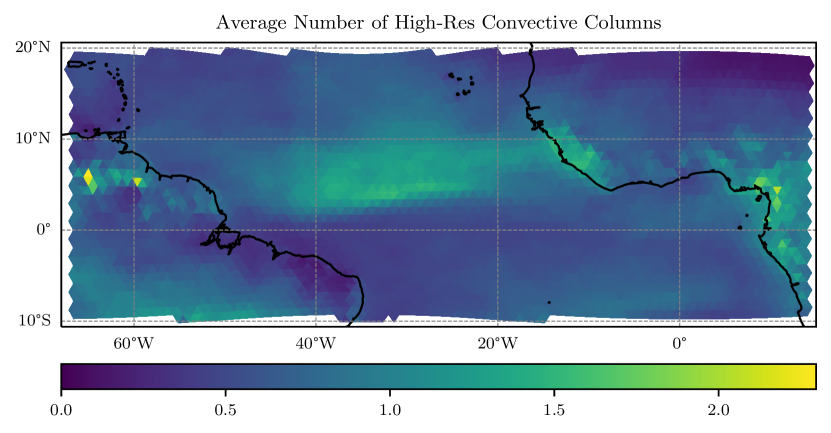
These simulations are well suited for learning a coarse-resolution data-driven convection scheme, as a high number of convective cases are present in the tropical Atlantic region. In Figure 1 the spatial distribution of the average number of convective cells per column (as defined below) in the studied region is shown. The figure shows a clear pattern of the ITCZ (compare \citeA[Fig. 2]RN58) with an increased number of convective cells. Additionally, many convective cells can be found along the coast and over mountainous terrain.
As a first preprocessing step we discarded the first hour of every day in the dataset because of some discontinuous behavior at the start of each day related to the initialization/spin-up phase of the simulations. Additionally, we also cropped the original NARVAL region by \qty2 on all sides since we noticed some boundary effects in the spatial patterns as well. The region seen in Figure 1 was already cropped by the mentioned \qty2.
To give a short overview of the preprocessing steps described below, Figure 2 depicts an overview of the various steps used, beginning with the original data set.
Computation of Output
The selection of input and output variables for the ML models are based on the implementation of the cumulus scheme in the ECHAM6 model [Tiedtke (\APACyear1989), Nordeng (\APACyear1994), Stevens \BOthers. (\APACyear2013)]. They correspond to the physical quantities transported by convective processes and a few related quantities such as precipitation. If not stated differently, we used the following set of variables for the input of the convective scheme
This set consists of the zonal, meridional, and vertical wind components (), as well as the moist static energy () and five different tracer species. These tracer species are the specific humidity () and specific cloud water, cloud ice, rain, and snow content (). The moist static energy is defined here as
| (1) |
with temperature , altitude , the specific heat at constant pressure , and the latent heat of evaporation and sublimation and .
Correspondingly, the output fields are
The first eight variables with notation “” are 3D fields and correspond to the subgrid flux component of the input variables (excluding ). The remaining variables in the output set are 2D fields, namely cloud top height (), cloud top pressure (), integrated liquid/ice detrainment (, ), and precipitation ().
We focused on predicting subgrid fluxes instead of the direct tendencies because this allowed abiding conservation laws by applying appropriate boundary conditions (no-flux at the top and a flux which is consistent with the surface forcing at bottom). We decomposed variables such as the density () into a horizontal spatial average over the coarse resolution, denoted by an overline, and a fluctuating component, denoted by a prime, as . The fluctuating component therefore represents the departure from the coarse grid average. This enabled us to calculate the subgrid (i.e., unresolved) vertical advective flux of, say, the variable , , for a given coarse resolution as follows:
| (2) |
This subgrid momentum flux was calculated as the difference between the coarse-grained flux obtained by first calculating the flux with the high-resolution resolved variables, then coarse-graining it to the coarser resolution, and the flux calculated with the low-resolution variables (see equation 2). The term on the right hand side in equation 2 results from the fact that averages over fluctuations are by definition zero. This method is similar to the one of \citeARN25, but without neglecting the horizontal density fluctuations between high resolution cells within a coarse resolution target cell of the coarse-graining procedure. This is especially important for models with terrain-following vertical coordinates, such as the height based terrain following vertical coordinate of the ICON model [Giorgetta \BOthers. (\APACyear2018)], because horizontally neighbouring cells (same vertical level) in the lower troposphere over land with steep topography can have strongly different height, thus different pressure and density. By looking into the subgrid variations of we found that, especially in the lowest levels over heterogeneous terrain, there are fluctuations of up to \qty25 of the mean value within a single coarse grid cell.
For the cloud top height/cloud top pressure (/) we took the height/pressure of the highest cell with convective clouds found according to the condition formulated in the next section (equation 4). The integrated detrainment of liquid/ice was calculated by first evaluating the fractional detrainment according to [Nordeng (\APACyear1994), Baba \BBA Giorgetta (\APACyear2020)],
| (3) |
where is the altitude and the fractional cloud area. As such, it was possible to calculate the integrated detrainment of water and ice by multiplication with the vertical mass flux and integrating along the column. Before integration, the column was masked according to its temperature (above or below \qty0) [Stevens \BOthers. (\APACyear2013)] to differentiate between liquid and ice detrainment. For convective columns we assumed that there is no stratiform precipitation present and that the precipitation stems entirely from convective clouds.
Coarse-Graining
The coarse-graining was done first in the horizontal and afterwards in the vertical direction as described in \citeARN24 for a data-driven cloud cover parameterization. The horizontal coarse-graining from the R2B10 () to an R2B5 () grid was performed with the help of the remapcon function from the Climate Data Operators (CDO) [Schulzweida (\APACyear2022)]. In the vertical, we reduced the resolution from to levels up to the mentioned limiting height of in Figure 3. The vertical coarse-graining operator works in a similar way as the horizontal averaging. The high-res cells were averaged weighted by their fractional proportion in the coarse cell [Grundner \BOthers. (\APACyear2022)]. Some low-resolution columns have a significantly lower base than the high-res cells because of the more detailed topography in the high-res data. Therefore, it was not possible to compute reasonable averages with the above described coarse-graining operator in the lowest model levels. Here, we also adopted the method from \citeARN24 and excluded columns with a significant difference between the vertical extent of low and high-resolution columns of the dataset.
In the high-resolution data, cells on the same vertical level can be on different geometric heights due to the terrain-following coordinate system. An approximation applied here is that the coarse-graining is first performed in the horizontal and afterwards in the vertical. Therefore the result can be different from coarse-graining over the low-res volume [Grundner \BOthers. (\APACyear2022)].
Additionally, we introduce time-averaging to reduce the noise from instantaneous snapshots of the dynamics [Ramadhan \BOthers. (\APACyear2020)]. For a column in the data set at time , we average the column variables and fluxes over the time steps , corresponding to a moving window of a three-hour duration.
Filtering for Convection
In order to learn mainly from columns in which convection has a dominant impact on the overall dynamics we introduced a filtering of the data. First, individual high resolution cells were classified as convective if the following conditions [Kirshbaum (\APACyear2022), Romps \BBA Charn (\APACyear2015)] are met:
| (4) |
where is the vertical velocity, is the virtual potential temperature, and / are the specific cloud liquid water/cloud ice content, respectively. Additionally, the buoyancy has been introduced in the conditions (4). In this case the overline denotes horizontal averaging over approximately \qty10\kilo. The averaging was performed with the remapcon function [Schulzweida (\APACyear2022)] to an R2B8 resolution. Next, we classified entire low resolution columns as convective or non-convective. For this, the number of convective cells per high resolution column was summed up along the height dimension and coarse-grained horizontally (as explained above). If the so-calculated 2D field was equal (or higher than) 1 for a given column, so that on average all high-res columns inside the coarse column had at least one convectively classified cell, this coarse column was classified as convective and was added to the training data set. These columns are henceforth referred to as “convective” columns. A time average over the entire observed period of this so computed low resolution data is displayed in Figure 1. Furthermore, we added of the non-convective columns for training so that we ended up with slightly more than \qty2million coarse sample columns. Before the filtering, there were about \qty5million low-res and approximately \qty455million high-res columns in the whole data set.
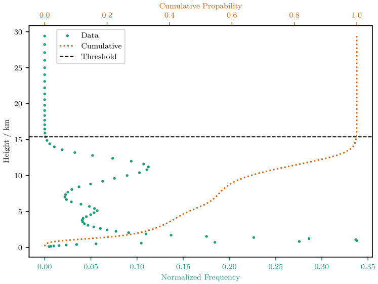
In order to find a limit in altitude to predict unresolved convective effects, we considered that convection in the atmosphere under normal conditions is limited by the tropopause [Shenk (\APACyear1974)]. Therefore, we checked up to which height we find convectively classified cells in the data set. The result can be seen in Figure 3. The limiting height in the figure is drawn at the height up to which \qty99.9 of the convectively classified cells are found (compare dashed orange line). This height is at , which is reasonable considering the tropical tropopause height of roughly [Gettelman \BOthers. (\APACyear2002)]. Only values below this height are considered as input and output to the machine learning algorithms.
The general form of the data observed in Figure 3 resembles the expected trimodal distribution of convective clouds in the tropics [Johnson \BOthers. (\APACyear1999)]. The lowest peak corresponds to (shallow) cumulus, the peak at to cumulus congestus and the highest clouds found are deep cumulonimbus clouds.
Rescaling and Normalization
For higher numerical stability of the machine learning models and to have the variables on the same scale, we standardize the 2D fields by subtracting the mean across samples from all 2D variables and dividing by the standard deviation. The same procedure is done for all 3D variables, but in this case mean and standard deviation are calculated across the height dimension as well.
Furthermore, before applying the standardization, we use the following nonlinear rescaling for the accumulated precipitation per hour:
| (5) |
The reason for this is that precipitation intensities are typically represented by a heavily skewed (gamma) distribution [Martinez-Villalobos \BBA Neelin (\APACyear2019)]. This distribution is characterized by a comparatively large number of low values and very few heavy precipitation events. Without a proper rescaling, ML models would achieve a low prediction error by predicting zero precipitation regardless of the input. Additionally, it is well known that coarse GCMs have a bias towards low intensity precipitation events [Moseley \BOthers. (\APACyear2016), Rasp \BOthers. (\APACyear2018)]. The rescaling should help mitigate some of this problem.
3 Machine Learning Models
As mentioned in the introduction, ML-based convection parameterizations have been developed using different kinds of methods. These include RFs [O’Gorman \BBA Dwyer (\APACyear2018), Yuval \BBA O’Gorman (\APACyear2020), Limon \BBA Jablonowski (\APACyear2023)], MLPs [Gentine \BOthers. (\APACyear2018), Rasp \BOthers. (\APACyear2018), Yuval \BOthers. (\APACyear2021), Iglesias-Suarez \BOthers. (\APACyear2023)], ensembles of MLPs [Krasnopolsky \BOthers. (\APACyear2013)], Convolutional Neural Networks (CNNs) [Han \BOthers. (\APACyear2020)], Generative Adversarial Networks (GANs) [Nadiga \BOthers. (\APACyear2022)], Residual Neural Networks (ResNets) [Wang \BOthers. (\APACyear2022)], and Variational Encoders (VAEs) / Variational Auto Encoder Decoders (VEDs) [Mooers \BOthers. (\APACyear2021), Behrens \BOthers. (\APACyear2022)]. One goal of this study is to evaluate various kinds of machine learning models on the same data set. Therefore, we first introduce the used models. All models use a vertical column (23 height levels and nine variables) from the sample data set as input and the column fluxes (23 height levels and eight variables) plus five variables as output, see above.
For the implementation of different ML models we used Scikit-Learn [Pedregosa \BOthers. (\APACyear2011)] and Pytorch [Paszke \BOthers. (\APACyear2019)]. As lowest complexity models we used linear methods such as Lasso [Tibshirani (\APACyear2018)] and Ridge [Hoerl \BBA Kennard (\APACyear1970)] regression. These methods are a form of linear regression with additional and regularization terms. We also compared three different models based on ensembles of decision trees: Random Forest (RF) [Breiman (\APACyear2001)], Extra Trees (ET) [Geurts \BOthers. (\APACyear2006)], and Gradient Boosted Trees (GBT) [Friedman (\APACyear2002)]. An RF is a collection of decision trees fitted on subsets of the training data and feature set. The ET model is based on the same principle but does not sub-sample the training data set, and the splitting of individual nodes in the trees is not based on the minimization of the error but it first splits at random points for random features and only afterwards chooses the best split among these candidates [Pedregosa \BOthers. (\APACyear2011)]. GBTs are a part of the more general family of Gradient Boosting algorithms. This family is based on ensembles of weak learners which are fitted iteratively to the residual of the previously fitted model with respect to the target data. In the case of GBTs, the class chosen as a weak learner is a decision tree. In this study we chose to use an implementation called the Histogram-based Gradient Boosting Regression Tree [Ke \BOthers. (\APACyear2017)]. This model is much faster for large data sets than classic GBTs because it bins the input data first, which makes the splitting step computationally much more efficient [Alsabti \BOthers. (\APACyear1998)]. Further information about the different ML models can be found in section References From the Supporting Information.
Besides these models, we used four different deep learning architectures: Multilayer Perceptron (MLP), Convolutional Neural Network (CNN), Residual Neural Network (ResNet) [He \BOthers. (\APACyear2016)], and U-Net [Ronneberger \BOthers. (\APACyear\bibnodate)]. The MLP family consists of several fully connected layers with additional optional batch normalization layers and activation functions (see section References From the Supporting Information). Furthermore, we introduced a linear model (LinMLP) which is based on the best found architecture of the MLP class but all nonlinear activation functions are replaced by linear ones. For the CNN class we decided to consider networks with a first convolutional layer connected to some number of fully connected layers thereafter. All convolutions are 1D convolutions in the vertical as the data set consists of variables on different levels due to the typical neglect of horizontal interactions and variability for parameterized processes in climate models. The ResNet architecture is inspired by \citeARN125, the network consists of several different blocks with some number of fully connected layers and optional batch normalization. The input of each block is added to its output to form the final output set. This helps prevent vanishing gradients and degradation [He \BOthers. (\APACyear2016)]. For the gradient-based optimization of the networks we chose to use the Adam algorithm [Kingma \BBA Ba (\APACyear2014)].
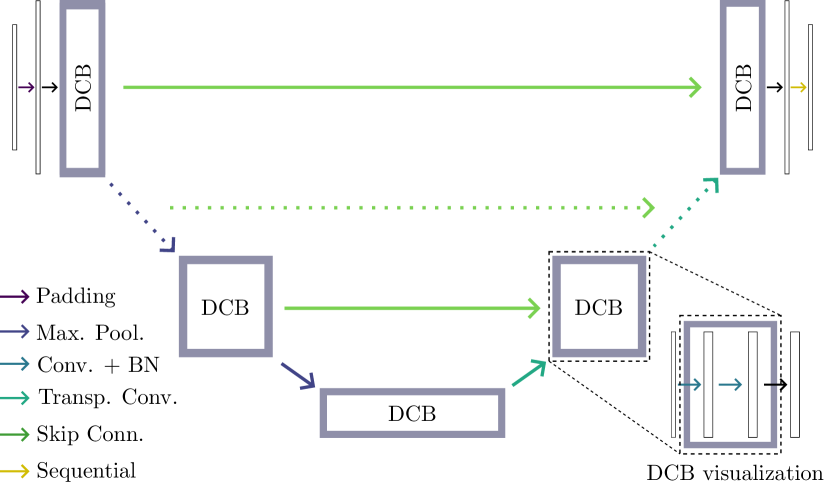
Finally, we decided to use a U-Net architecture, see Figure 4. This network is similar to the ResNet in the sense that it contains residual connections and that it is constructed out of structurally similar blocks. In contrast to the ResNet, these blocks use two convolutional layers each instead of an arbitrary number of fully connected layers. Additionally, this architecture utilizes max pooling and transpose convolution layers to compress and expand the input in the height dimension. This allows the network to process the input information on multiple spatial scales. During the compression process (left part of Figure 4) the channel dimension (width in the figure) grows. In the expansion process (right part) the channel dimension shrinks again. We propose this architecture, which is particularly suited for multiscale modeling, for the given parameterization problem because of the multiscale nature of moist convection [Majda (\APACyear2007)]. The U-Net has favorable properties as local features can be picked up by the network on a variety of different scales throughout the downscaling process, and the residual connections help to communicate this information to the upscale branch of the network.
To select an appropriate set of hyperparamters we chose to split the data non-consecutively into a training/validation/test set with a fraction of \qty80/\qty10/\qty10 of the data. This corresponds to sample columns for training and columns for validation/testing. For the non-deep learning algorithms we first did the HPO on a subset of the data from five random days because most of the models have difficulties with handling vast amount of data. The models identified as best in the HPO where then trained on the whole data set. An explanation of the different hyperparameters involved in all models can be found in section References From the Supporting Information.
4 Results
This section will first introduce a model evaluation for all ML models used and then focus on a more detailed comparison of the highest performing deep and non-deep learning method. In the end, we will explain the model predictions and the differing performances between the methods.
First, we focus on the simple aggregated evaluation of the coefficient of determination () values for all examined model classes. The value is calculated as 1 minus the mean squared error of the predictions over the variance of the data. We compute the value across variables and levels, a more detailed (per variable/level) comparison is given later in Figure 8. All models have been hyperparameter-tuned according to the method described below. Briefly this HPO consisted of running a large ensemble of models with parameters sampled from predefined search spaces and their performance evaluated on a validation set (more details in section References From the Supporting Information).
Figure 5 displays the values for all models over all variables and levels. On the left hand side of the dashed green line the deep learning models are shown as opposed to the simpler models on the right hand side.
The value of the Random Forest is the lowest of the examined models. RFs have been used as data-driven convection parameterizations with some success [O’Gorman \BBA Dwyer (\APACyear2018), Yuval \BBA O’Gorman (\APACyear2020)] in idealized settings before. Limitations in the application of RFs for realistic parameterization schemes have been observed before due to their computational inefficiency, memory requirements, and comparably low complexity (versus deep neural networks for instance), limiting their capacity to capture high dimensional features [Limon \BBA Jablonowski (\APACyear2023)]. The GBT model class has a strikingly high value, comparable to the ones of the deep learning methods. This suggests that these RF-based parameterization schemes could improve in performance if they were based on Gradient Boosted Trees (besides deep learning networks). The Extra Trees model has a similarly low performance as the RF. Considering that the ET model is structurally similar to RFs, including an additional element of randomness as explained above, this is not surprising. The linear models (Ridge, LinMLP, and Lasso) show relatively high performance compared to that of the RF/ET model with values of . The -regularization term seems to have a higher impact on the generalization capabilities of the linear model compared to the -regularization in Lasso regression.
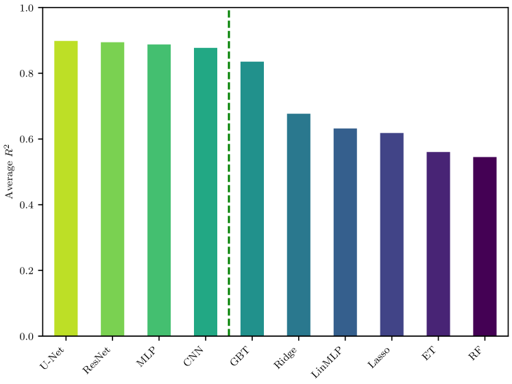
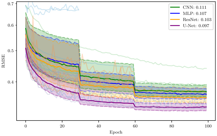
The deep learning models outperform the other methods but, e.g., for the GBT model only by a small amount. While the value for the GBT is almost as high as the value for the U-Net, the other nonlinear methods show a rapid decrease in performance when ordering by their respective value. Figure 5 shows that the performance difference between the various deep learning models measured by is negligible. One could suspect that the best performance of the U-Net could originate purely by chance. Therefore, we performed an extensive HPO with over ensemble members in total. The resulting median/upper/lower quartile profiles can be seen in Figure 6. We varied hyperparameters such as the learning rate, number of neurons/layers/blocks, or activation functions. More details on the HPO search spaces can be found in section References From the Supporting Information. A visualization of the HPO and the training and validation process in general is shown in Figure References From the Supporting Information. We notice that the U-Net has a consistently lower error than the other models, and the upper quartile of its distribution is on the same level as the lower quartile of the second best performing model, the ResNet. The difference between the other model classes is smaller, and the spread around each median profile is larger than for the U-Net.
Furthermore, the model complexity of the U-Net is comparatively low. As it can be seen in Table References From the Supporting Information and Figure References From the Supporting Information, the most complex (judging by number of parameters) deep learning model is the ResNet with more than four times the number of parameters of the U-Net. The MLP architecture has the lowest number of parameters, the U-Net has the second lowest number before the CNN and ResNet. Despite this, the U-Net shows the lowest error on the validation/test set, presumably because of its multiscale architecture and the resulting ability to capture multiscale problems such as turbulence well.
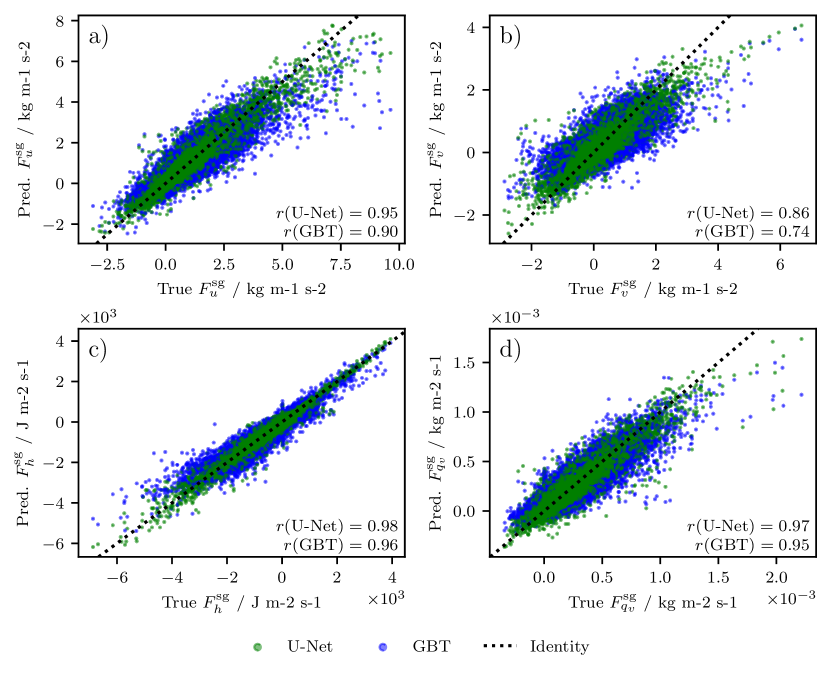
Based on these results, we will focus on the respectively best performing deep and non-deep learning models from now on. These models are the U-Net and the GBT model as seen in Figure 5. We first compare the U-Net and GBT flux predictions with the true values for over all levels. The results can be seen in Figure 7, and a corresponding plot showing the distribution for the remaining tracer subgrid fluxes can be seen in Figure References From the Supporting Information. The correlation is always higher for the U-Net predictions, and for both models the meridional momentum fluxes are the hardest to predict. Especially for high values of the flux, both models tend to underestimate the true flux, which can be seen by the points below the diagonal in plot b). To a similar extent, this trend can also be seen for the fluxes and . The mentioned fluxes of the GBT show a slight corresponding overestimation for low flux values. In contrast to that, the U-Net data distribution is more symmetric about the main diagonal. This means that there is no or a very small systematic under- or over-prediction for these values by the U-Net. In general, the spread around the diagonal is bigger for the GBT than for the U-Net. This confirms the better performance of the U-Net seen in Figure 5 based on values.
After having examined the model performance aggregated over all levels we now look at the average values of the 3D variables on individual vertical levels. This is shown in Figure 8, again for the U-Net and GBT. Some vertical levels are not shown in the figure because the variation of the variables on these levels is close to zero. We determined the variables for which this is true by first finding the th percentile of their absolute values. Then, for each variable all levels in which the computed percentile is below \qty1 of the maximum percentile for the variable were excluded from the plot.
This method filters all levels which show significantly less variation compared to all other levels. Looking at Figure 8 we filtered out the lower tropospheric values for the ice and snow tracers as well as the higher tropospheric values for cloud water and rain tracers. This is reasonable because we do not expect much snow/ice in the lower troposphere of the tropics, and similarly, the temperatures are too low for cloud water/rain to exist close to the tropopause.
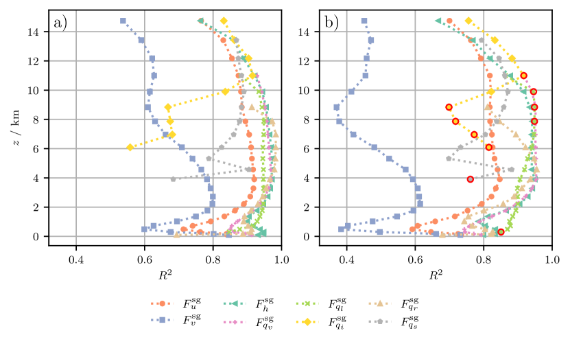
Comparing the plots in Figure 8, the two models show similar patterns as seen, e.g., for the curve, but the GBT curves are mostly shifted towards lower values compared to the U-Net. For most variables we find a clear advantage of the U-Net in the upper layers and around the height of the planetary convective boundary layer at . Other than for tracer species on levels in which the corresponding concentration is typically very low, the models show difficulties to predict the subgrid momentum fluxes compared to other variables, as is particularly visible for . For subgrid momentum transport in general this has been noticed before in \citeARN145. This problem could arise from the fact that the sign of the subgrid convective momentum flux depends on the nature of convective organization [Yuval \BBA O’Gorman (\APACyear2023), LeMone (\APACyear1983)], which is not resolved in the coarse data. A few points are marked by red circles, which correspond to higher value for the GBT. Most of these are close to the U-Net value (within an relative deviation of \qty1.5) except for the low ice and snow tracer values. Here we assume that the GBT shows an increased performance due to the small number of training data and its lower model complexity. Using the U-Net increases the mean value of all variables. The highest improvement by using the U-Net instead of the GBT can be seen for with an average improvement of and the second highest for with a gain of . In the vertical, the highest average increase in skill is observed in the boundary layer. On these lower model levels, the dynamics are typically more complex/turbulent and therefore the higher model complexity of the U-Net is especially beneficial.
The 2D fields are also predicted more skillfully by the U-Net, the values for all five predicted 2D variables are higher for the U-Net than for the GBT. As an example, the true and predicted precipitation distribution is shown in Figure References From the Supporting Information. Even though the values for precipitation are similar ( vs. ), the U-Net predicts the extremes of the distribution much more accurately. For instance, the 95th percentile of the true distribution and the predicted distributions of U-Net and GBT are approximately \qty22.28\milli\per, \qty19.75\milli\per, and \qty16.83\milli\per. This shows that the U-Net captures the high precipitation cases much better than the GBT.
Looking at the spatial distribution of the normalized RMSE across all variables (see Figure References From the Supporting Information) we notice that both models have a lower error in the region of the ITCZ and an increase in error towards higher latitudes. This reflects the difference in the abundance of training data as seen in Figure 1.
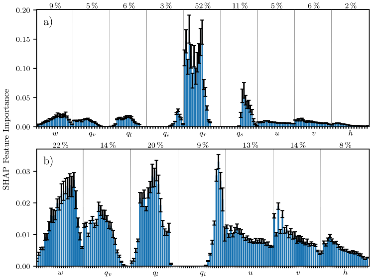
Having looked into the prediction results we now want to find out what the models actually have learned in order to predict the parameterization output. This will be based on the SHapley Additive exPlanations (SHAP) [Lundberg \BBA Lee (\APACyear2017)] library which analyzes ML model predictions using a game theoretic approach. A SHAP value gives the deviation in an output variable due to a specific value of the variable from the average prediction of over a given data (sub)set . We used the DeepExplainer class [Lundberg \BBA Lee (\APACyear2017)] as an efficient explainer for deep neural networks, and the TreeExplainer/KernelExplainer class for decision tree-based models such as GBT. Figure 9 a) shows the mean absolute values of the calculated SHAP values for the U-Net model. These correspond to feature importances and in this case show that the model mainly focuses on using the precipitating tracer species to predict the subgrid fluxes. The top plot shows that dominates the importance attribution with over \qty50 of all values. As second most influential feature we see , another precipitating tracer species, even though it is only highly influential in the upper layers. Additionally, one notices that the standard deviation is relatively large for /, indicating the ambiguity of the learned relations. This is a first hint that the model learned non-causal relationships between convective precipitation and convective subgrid fluxes. When the model “sees” coarse-grained precipitation in the data it predicts that convective subgrid fluxes must be present. This behavior can also be observed in a more detailed analysis of the SHAP values (Figure References From the Supporting Information).
To prevent the model from learning these non-causal connections we trained another set of models with less input variables. We left out the precipitation input tracer species and . For this ablated model versions we performed a new HPO. These models will be discussed henceforth. The performance of both models (U-Net and GBT) on the test set decreases marginally, by , by ablating the precipitating tracers as inputs. A third HPO was performed neglecting horizontal density fluctuations, with the result that the validation error increased for all model classes by about \qty4, and for the MLP only negligibly. This is a hint that the irreducible error of the models increases by neglecting density fluctuations.
The feature importances for the ablated U-Net are displayed in plot b) of Figure 9. A more spread-out feature importance assignment can be seen in this plot: the difference between highest and lowest valued feature is only \qty14 which is much less than \qty50 as before. This model now relies less on spurious correlations between precipitation and convective subgrid fluxes and should generalize better outside the training domain. The general trend for most variables seen in Figure 9 indicates that the model focuses more on the lower model levels, and the importance is decreasing with height. For , , and this is not the case, the feature importance peaks at higher model levels. The specific cloud ice content is only present at higher altitudes as already discussed. For the cloud water content we have very low concentrations at low model levels as clouds generally form in the boundary layer during daytime [Stull (\APACyear1988)], and the mean vertical velocity profile also shows higher values at greater altitudes, indicative of the importance of shear such as on mesoscale convective system organization [Rotunno \BOthers. (\APACyear1988)].
We looked at the feature importance in Figure 9 but did not discuss the influence of an input on the various output variables. For this, we now first explain the method and then discuss the results. For ease of notation, we focus here on a single output model with output variable as before, but this can easily be generalized to higher dimensional output. To get the average effect of an input variable on the output variable we first define the fluctuation of for sample as , where the brackets denotes the average value over in the set . The data set is a random subset of the whole data set as to save computational costs. Now, we define the normalized fluctuation as
| (6) |
The weighted average effect of on can now be quantified in a similar way as in \citeA2021arXiv211208440B in a vector , with
| (7) |
A positive expresses an increasing/decreasing for an increasing/decreasing independently of other values, and for a negative we have the opposite effect. For a multi-output model this vector becomes a 2D matrix quantifying the influence of the th input on the th output. We will refer to the SHAP values obtained by this method as weighted SHAP values from now on.
Applying this method to the trained U-Net model gives the matrix visualized in Figure 10. We see many interpretable, local influences (main diagonal patterns) in this figure, for example a mainly positive influence of cloud liquid water on /. This learned correlation can be understood by looking at the condensation process of water vapour. When water condenses in an atmospheric grid cell, latent heat is released and the air becomes more buoyant. The more water condenses, the more buoyant the air parcels get and increased convective fluxes are initiated. For specific humidity the opposite effect is visible (controlling for ) on the convective subgrid fluxes of /. As previously observed \citeAbeucler_et_al_ALinearResponse, this local drying effect is plausibly related to the entrainment of water vapor into the plume. Furthermore, we see a slightly positive impact and moistening flux of the lower model levels on higher levels. This is indicative of the decrease in air density for increased water vapor content and the decreased lapse rate for buoyant air parcels (and therefore higher convective instability).
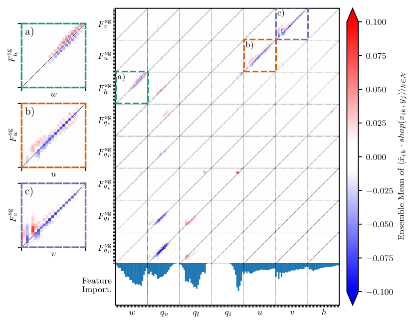
Apart from that, the main visible signatures are visualized in the insets of Figure 10. Inset a) shows the influence of on . The main pattern is in the upper layers where we can see primarily a positive super- and negative sub-diagonal ( with and , respectively). This means that cells with a high vertical velocity have a positive influence on the subgrid flux in the cell above them and a negative influence below them respectively. Considering that mesoscale convergence and large scale ascent can initiate/enforce convective cells [Kalthoff \BOthers. (\APACyear2009)], this seems reasonable. In Inset b), a negative diagonal pattern can be observed. A high horizontal wind speed in a cell leads to the horizontal transport of a possible convective plume to an adjacent region, so that it reduces the convective subgrid flux in the considered column. This explains the main diagonal. Otherwise, we see a positive area above the diagonal, mainly in the lower part of the plot. Consequently, high horizontal wind speeds imply a positive horizontal momentum flux in the cells above, as it gets transported by convection upwards. We also see a positive pattern in the sub-diagonal for higher levels. These patterns can be explained by forced convect, ion and the general impact of shear on organized mesoscale convective systems. Vertical wind shear has been found to be an essential ingredient for long-lived and well-organized convective storm cells [Rotunno \BOthers. (\APACyear1988), Doswell \BBA Evans (\APACyear2003), Roca \BOthers. (\APACyear2017)]. A very similar pattern can be observed in Inset c), the main difference is that for lower levels there are a few non-local transport signatures. These patterns are consistent (with relative standard deviations of max ) over different realizations of so that the result here seems not to be dependent on the set .
As a comparison, the corresponding weighted SHAP values for the GBT are displayed in Figure 11. First, the GBT feature importances have a much less regular pattern and look more “randomly” distributed. These patterns show a less coherent picture and are not so easily interpretable. Looking at the aggregated feature importance, both models weigh the moist static energy the least. The GBT model weighs the specific humidity higher in its predictions with an aggregated importance of \qty29 compared to the U-Net with \qty14. As most important features for the U-Net, on the other hand, we have the vertical velocity and cloud water content . These two variables are also part of the condition formulated in equation 4 for convective conditions in a grid cell. Therefore, it is reasonable that the network learns to pay attention to these inputs.
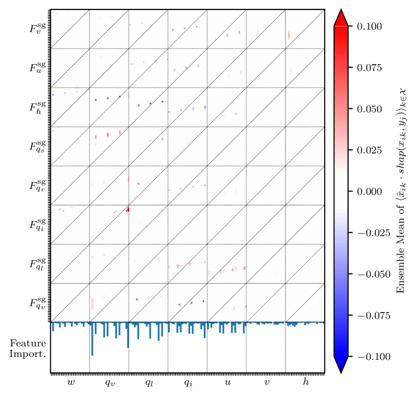
Since the weighted SHAP values displayed in Figure 10 consistently show vastly different patterns than in Figure 11, we used the same method for the RF as well and got a similar picture to what is displayed here for the GBT. In order to rule out a dependence of the obtained results on the Shapley value approximation method, we also used the KernelExplainer [Lundberg \BBA Lee (\APACyear2017)] as an alternative to the TreeExplainer. The resulting weighted SHAP values have almost the same form as for the TreeExplainer class, emphasizing that our results are independent of the explanation method. We also looked at the standard deviations of all weighted SHAP value plots and observed that the uncertainty is very low compared to the mean values shown (The maximum deviation is , and \qty99 of the standard deviation values are below ), further demonstrating that those interpretation statistics are stable across samples.
For the data in Figure 10, these values are and , respectively. Looking at the scales in both figures, these uncertainties are very small.
Overall, this indicates that although the predictive performance of the GBT is comparable to that of the U-Net, it relies on very different statistical patterns in the data. These patterns are more non-local and mostly unphysical so that the resulting model is expected to have less skill in extrapolating outside its training domain.
5 Conclusions and Discussion
In order to develop an ML-based parameterization for convection we first filtered, processed, and coarse-grained data from high resolution simulations with explicit convection. To separate convection from other processes, we used a filtering method for convective conditions. That ensures that the ML models learn mostly convective fluxes. We then coarse-grained the high-resolution data to the target resolution and calculated the subgrid fluxes of the needed output quantities. The coarse-graining was performed without neglecting horizontal density fluctuations since we used data from a model with terrain following coordinates and the irreducible error increases if the model does not have the necessary input information.
We found that the U-Net architecture is a very suitable machine learning model to parameterize convective subgrid fluxes, which is naturally a multiscale process. The U-Net outperformed other deep learning models by only a small margin judging by the metric. However, comparing the performance over a broad range of parameters, the error of the U-Net was consistently lower than the error of MLP, CNN, and ResNet architectures. A comparatively lower is achieved by most non-deep-learning models except for the Gradient Boosting Trees model. This GBT model had a coefficient of determination of compared to the U-Net with . Nonetheless, in a direct comparison between GBT and U-Net, the best performing non-deep learning and deep learning model, the U-Net had an advantage in almost all aspects. An exception to this is shown in Figure 3 by the value for a few levels for ice, snow, and cloud water tracers. For snow and ice these exceptions occurred in the lower levels and for cloud liquid water mainly in the higher ones, where the respective tracer species are rarely observed / have a very low concentration. This demonstrates the advantage of the lower complexity tree-based method for sparse data or rather for regions where an interpolation based on few relevant samples is needed. For the other levels and also for the predicted 2D fields, such as convective precipitation, we noticed a clear benefit of using the U-Net architecture.
To get some insight into what the model exactly learned during training we applied the SHAP framework and first calculated feature importances. These revealed that the U-Net model focuses strongly on the precipitating tracer species rain and snow as input variables. Here, the SHAP values exposed that the model learned non-causal relations between convective subgrid fluxes and convective precipitation. This was also seen in the figure showing the weighted SHAP values (References From the Supporting Information), as particularly the rain tracers showed heavy non-local influences on subgrid fluxes for moist static energy, rain, cloud liquid, and water vapor tracers. As a result we performed the same analysis on an ablated model without water species. A potential solution to be investigated in a future study would be to restrict the model to learn causal relationships as in \citeA2023arXiv230412952I. Another approach to improve the predictions of subgrid momentum fluxes specifically would be to model the degree of small scale convective organization [Shamekh \BOthers. (\APACyear2023)]. For coupling the developed ML-based multi scale parameterization to a GCM it could be necessary to use a global training data set.
By looking at the weighted SHAP values we found that the ablated version of the U-Net was more physical and learned physically explainable connections between coarse-scale variables and subgrid fluxes. For example, there were patterns of local upwards transport of horizontal momentum and energy, phase change (latent heat flux) patterns, and signs of convective forcing. This strengthens trust in the model as it can be expected to extrapolate better to data outside its training domain. This extrapolation capability has only been tested for data originating from the same set of simulations, in future work the degree of extrapolation power will be tested on more diverse data sets. Coupling the resulting schemes to the ICON climate model will further show whether the expected generalization power will hold sufficiently. The weighted SHAP values for the GBT model, on the other hand, were not physically interpretable as they showed scattered results. We applied a different explainer class to test the robustness of this outcome and saw consistent results. To investigate this further, we did the same analysis for the Random Forest as this model has been used in other studies before. Here, the weighted SHAP values were similarly scattered as for the GBT model. This result shows that seemingly well performing models (judging by e.g. ) can in fact rely on non-causal correlations in the data, achieving good results for the “wrong reasons”. Therefore, these models are most likely not suited for the coupling to a GCM.
Our study leads to the conclusion that interpretability/explainability of ML algorithms is important to investigate potentially unphysical mechanisms. Furthermore, we conclude that the U-Net is the best choice of the examined model classes as it is very accurate, not too complex, and its predictions can be explained physically. This advantage over other ML-model classes likely comes from the ability of the U-Net to capture multiscale phenomena like convection.
Open Research
Code will be published under https://github.com/EyringMLClimateGroup/heuer23_ml_convection_parameterization. The simulation data used to train and evaluate the machine learning algorithms amounts to several TB and can be reconstructed with the scripts provided in the GitHub repository. Access to the NARVAL data set was provided by the German Climate Computing Center (DKRZ) The software code for the ICON model is available from https://code.mpimet.mpg.de/projects/iconpublic.
Acknowledgements.
Funding for this study was provided by the European Research Council (ERC) Synergy Grant “Understanding and Modelling the Earth System with Machine Learning (USMILE)” under the Horizon 2020 research and innovation programme (Grant agreement No. 855187). This work used resources of the Deutsches Klimarechenzentrum (DKRZ) granted by its Scientific Steering Committee (WLA) under project ID bd1179. The authors gratefully acknowledge the Earth System Modelling Project (ESM) for funding this work by providing computing time on the ESM partition of the supercomputer JUWELS [Jülich Supercomputing Centre (\APACyear2021)] at the Jülich Supercomputing Centre (JSC). Furthermore, we thank the authors of \citeARN57 for creating and providing the high-res simulations of the tropical Atlantic used in this study. We also thank E. Haslauer for careful reading of the paper and his valuable feedback.References
- Alsabti \BOthers. (\APACyear1998) \APACinsertmetastar10.5555/3000292.3000294{APACrefauthors}Alsabti, K., Ranka, S.\BCBL \BBA Singh, V. \APACrefYearMonthDay1998. \BBOQ\APACrefatitleCLOUDS: A Decision Tree Classifier for Large Datasets CLOUDS: A decision tree classifier for large datasets.\BBCQ \BIn \APACrefbtitleProceedings of the Fourth International Conference on Knowledge Discovery and Data Mining Proceedings of the fourth international conference on knowledge discovery and data mining (\BPG 2–8). \APACaddressPublisherAAAI Press. \PrintBackRefs\CurrentBib
- Anber \BOthers. (\APACyear2015) \APACinsertmetastardoi:10.1073/pnas.1505077112{APACrefauthors}Anber, U., Gentine, P., Wang, S.\BCBL \BBA Sobel, A\BPBIH. \APACrefYearMonthDay2015. \BBOQ\APACrefatitleFog and rain in the Amazon Fog and rain in the amazon.\BBCQ \APACjournalVolNumPagesProceedings of the National Academy of Sciences1123711473-11477. {APACrefDOI} 10.1073/pnas.1505077112 \PrintBackRefs\CurrentBib
- Arakawa \BBA Schubert (\APACyear1974) \APACinsertmetastarRN59{APACrefauthors}Arakawa, A.\BCBT \BBA Schubert, W\BPBIH. \APACrefYearMonthDay1974. \BBOQ\APACrefatitleInteraction of a cumulus cloud ensemble with the large-scale environment, Part I Interaction of a cumulus cloud ensemble with the large-scale environment, part i.\BBCQ \APACjournalVolNumPagesJournal of the atmospheric sciences313674-701. \PrintBackRefs\CurrentBib
- Baba \BBA Giorgetta (\APACyear2020) \APACinsertmetastarRN50{APACrefauthors}Baba, Y.\BCBT \BBA Giorgetta, M\BPBIA. \APACrefYearMonthDay2020. \BBOQ\APACrefatitleTropical Variability Simulated in ICON‐A With a Spectral Cumulus Parameterization Tropical variability simulated in ICON‐A with a spectral cumulus parameterization.\BBCQ \APACjournalVolNumPagesJournal of Advances in Modeling Earth Systems121e2019MS001732. \PrintBackRefs\CurrentBib
- Behrens \BOthers. (\APACyear2022) \APACinsertmetastarRN88{APACrefauthors}Behrens, G., Beucler, T., Gentine, P., Iglesias-Suarez, F., Pritchard, M.\BCBL \BBA Eyring, V. \APACrefYearMonthDay2022. \BBOQ\APACrefatitleNon-Linear Dimensionality Reduction With a Variational Encoder Decoder to Understand Convective Processes in Climate Models Non-linear dimensionality reduction with a variational encoder decoder to understand convective processes in climate models.\BBCQ \APACjournalVolNumPagesJournal of Advances in Modeling Earth Systems148e2022MS003130. \APACrefnotee2022MS003130 2022MS003130 {APACrefDOI} https://doi.org/10.1029/2022MS003130 \PrintBackRefs\CurrentBib
- Beucler \BOthers. (\APACyear2018) \APACinsertmetastarbeucler_et_al_ALinearResponse{APACrefauthors}Beucler, T., Cronin, T.\BCBL \BBA Emanuel, K. \APACrefYearMonthDay2018. \BBOQ\APACrefatitleA Linear Response Framework for Radiative-Convective Instability A linear response framework for radiative-convective instability.\BBCQ \APACjournalVolNumPagesJournal of Advances in Modeling Earth Systems1081924-1951. {APACrefDOI} https://doi.org/10.1029/2018MS001280 \PrintBackRefs\CurrentBib
- Beucler \BOthers. (\APACyear2021) \APACinsertmetastar2021arXiv211208440B{APACrefauthors}Beucler, T., Pritchard, M., Yuval, J., Gupta, A., Peng, L., Rasp, S.\BDBLGentine, P. \APACrefYearMonthDay2021. \BBOQ\APACrefatitleClimate-Invariant Machine Learning Climate-Invariant Machine Learning.\BBCQ \APACjournalVolNumPagesarXiv e-printsarXiv:2112.08440. {APACrefDOI} 10.48550/arXiv.2112.08440 \PrintBackRefs\CurrentBib
- Bock \BOthers. (\APACyear2020) \APACinsertmetastarBock2020{APACrefauthors}Bock, L., Lauer, A., Schlund, M., Barreiro, M., Bellouin, N., Jones, C.\BDBLEyring, V. \APACrefYearMonthDay2020. \BBOQ\APACrefatitleQuantifying Progress Across Different CMIP Phases With the ESMValTool Quantifying progress across different CMIP phases with the ESMValTool.\BBCQ \APACjournalVolNumPagesJournal of Geophysical Research: Atmospheres12521. {APACrefDOI} 10.1029/2019jd032321 \PrintBackRefs\CurrentBib
- Breiman (\APACyear2001) \APACinsertmetastarBreiman2001{APACrefauthors}Breiman, L. \APACrefYearMonthDay2001. \BBOQ\APACrefatitleRandom Forests Random forests.\BBCQ \APACjournalVolNumPagesMachine Learning4515-32. {APACrefDOI} 10.1023/A:1010933404324 \PrintBackRefs\CurrentBib
- Brenowitz \BOthers. (\APACyear2020) \APACinsertmetastarRN143{APACrefauthors}Brenowitz, N\BPBID., Beucler, T., Pritchard, M.\BCBL \BBA Bretherton, C\BPBIS. \APACrefYearMonthDay2020. \BBOQ\APACrefatitleInterpreting and stabilizing machine-learning parametrizations of convection Interpreting and stabilizing machine-learning parametrizations of convection.\BBCQ \APACjournalVolNumPagesJournal of the Atmospheric Sciences77124357-4375. \PrintBackRefs\CurrentBib
- Brenowitz \BBA Bretherton (\APACyear2018) \APACinsertmetastarRN107{APACrefauthors}Brenowitz, N\BPBID.\BCBT \BBA Bretherton, C\BPBIS. \APACrefYearMonthDay2018. \BBOQ\APACrefatitlePrognostic validation of a neural network unified physics parameterization Prognostic validation of a neural network unified physics parameterization.\BBCQ \APACjournalVolNumPagesGeophysical Research Letters45126289-6298. \PrintBackRefs\CurrentBib
- Ceppi \BBA Nowack (\APACyear2021) \APACinsertmetastarRN159{APACrefauthors}Ceppi, P.\BCBT \BBA Nowack, P. \APACrefYearMonthDay2021. \BBOQ\APACrefatitleObservational evidence that cloud feedback amplifies global warming Observational evidence that cloud feedback amplifies global warming.\BBCQ \APACjournalVolNumPagesProceedings of the National Academy of Sciences11830e2026290118. {APACrefDOI} doi:10.1073/pnas.2026290118 \PrintBackRefs\CurrentBib
- Christopoulos \BBA Schneider (\APACyear2021) \APACinsertmetastarRN165{APACrefauthors}Christopoulos, C.\BCBT \BBA Schneider, T. \APACrefYearMonthDay2021. \BBOQ\APACrefatitleAssessing Biases and Climate Implications of the Diurnal Precipitation Cycle in Climate Models Assessing biases and climate implications of the diurnal precipitation cycle in climate models.\BBCQ \APACjournalVolNumPagesGeophysical Research Letters4813e2021GL093017. {APACrefDOI} https://doi.org/10.1029/2021GL093017 \PrintBackRefs\CurrentBib
- Collins \BOthers. (\APACyear2006) \APACinsertmetastarCAM3{APACrefauthors}Collins, W\BPBID., Rasch, P\BPBIJ., Boville, B\BPBIA., Hack, J\BPBIJ., McCaa, J\BPBIR., Williamson, D\BPBIL.\BDBLZhang, M. \APACrefYearMonthDay2006. \BBOQ\APACrefatitleThe Formulation and Atmospheric Simulation of the Community Atmosphere Model Version 3 (CAM3) The formulation and atmospheric simulation of the community atmosphere model version 3 (CAM3).\BBCQ \APACjournalVolNumPagesJournal of Climate19112144 - 2161. {APACrefDOI} https://doi.org/10.1175/JCLI3760.1 \PrintBackRefs\CurrentBib
- Doswell \BBA Evans (\APACyear2003) \APACinsertmetastarDOSWELL2003117{APACrefauthors}Doswell, C\BPBIA.\BCBT \BBA Evans, J\BPBIS. \APACrefYearMonthDay2003. \BBOQ\APACrefatitleProximity sounding analysis for derechos and supercells: an assessment of similarities and differences Proximity sounding analysis for derechos and supercells: an assessment of similarities and differences.\BBCQ \APACjournalVolNumPagesAtmospheric Research67-68117-133. \APACrefnoteEuropean Conference on Severe Storms 2002 {APACrefDOI} https://doi.org/10.1016/S0169-8095(03)00047-4 \PrintBackRefs\CurrentBib
- Eyring, Gillett\BCBL \BOthers. (\APACyear2021) \APACinsertmetastarEyring2021{APACrefauthors}Eyring, V., Gillett, N., Rao, K\BPBIA., Barimalala, R., Parrillo, M\BPBIB., Bellouin, N.\BDBLSun, Y. \APACrefYearMonthDay2021. \BBOQ\APACrefatitleClimate Change 2021: The Physical Science Basis. Contribution of Working Group I to the Sixth Assessment Report of the Intergovernmental Panel on Climate Change Climate change 2021: The physical science basis. contribution of working group i to the sixth assessment report of the intergovernmental panel on climate change.\BBCQ \BIn V. Masson-Delmotte \BOthers. (\BEDS), (\BPG 423–552). \APACaddressPublisherCambridge University Press, Cambridge, United Kingdom and New York, NY, USA. {APACrefDOI} 10.1017/9781009157896.005 \PrintBackRefs\CurrentBib
- Eyring, Mishra\BCBL \BOthers. (\APACyear2021) \APACinsertmetastarEyring2021a{APACrefauthors}Eyring, V., Mishra, V., Griffith, G\BPBIP., Chen, L., Keenan, T., Turetsky, M\BPBIR.\BDBLvan der Linden, S. \APACrefYearMonthDay2021. \BBOQ\APACrefatitleReflections and projections on a decade of climate science Reflections and projections on a decade of climate science.\BBCQ \APACjournalVolNumPagesNature Climate Change114279–285. {APACrefDOI} 10.1038/s41558-021-01020-x \PrintBackRefs\CurrentBib
- Forster \BOthers. (\APACyear2021) \APACinsertmetastarAR6WG1CH7{APACrefauthors}Forster, P., Storelvmo, T., Armour, K., Collins, W., Dufresne, J\BHBIL., Frame, D.\BDBLZhang, H. \APACrefYearMonthDay2021. \BBOQ\APACrefatitleThe Earth’s Energy Budget, Climate Feedbacks, and Climate Sensitivity The earth’s energy budget, climate feedbacks, and climate sensitivity\BBCQ [Book Section]. \BIn V. Masson-Delmotte \BOthers. (\BEDS), \APACrefbtitleClimate Change 2021: The Physical Science Basis. Contribution of Working Group I to the Sixth Assessment Report of the Intergovernmental Panel on Climate Change Climate change 2021: The physical science basis. contribution of working group i to the sixth assessment report of the intergovernmental panel on climate change (\BPG 923–1054). \APACaddressPublisherCambridge, United Kingdom and New York, NY, USACambridge University Press. {APACrefDOI} 10.1017/9781009157896.009 \PrintBackRefs\CurrentBib
- Friedman (\APACyear2002) \APACinsertmetastarFRIEDMAN2002367{APACrefauthors}Friedman, J\BPBIH. \APACrefYearMonthDay2002. \BBOQ\APACrefatitleStochastic gradient boosting Stochastic gradient boosting.\BBCQ \APACjournalVolNumPagesComputational Statistics & Data Analysis384367-378. \APACrefnoteNonlinear Methods and Data Mining {APACrefDOI} https://doi.org/10.1016/S0167-9473(01)00065-2 \PrintBackRefs\CurrentBib
- Gentine \BOthers. (\APACyear2018) \APACinsertmetastarRN5{APACrefauthors}Gentine, P., Pritchard, M., Rasp, S., Reinaudi, G.\BCBL \BBA Yacalis, G. \APACrefYearMonthDay2018. \BBOQ\APACrefatitleCould Machine Learning Break the Convection Parameterization Deadlock? Could machine learning break the convection parameterization deadlock?\BBCQ \APACjournalVolNumPagesGeophysical Research Letters45115742-5751. {APACrefDOI} https://doi.org/10.1029/2018GL078202 \PrintBackRefs\CurrentBib
- Gettelman \BOthers. (\APACyear2002) \APACinsertmetastarRN146{APACrefauthors}Gettelman, A., Salby, M\BPBIL.\BCBL \BBA Sassi, F. \APACrefYearMonthDay2002. \BBOQ\APACrefatitleDistribution and influence of convection in the tropical tropopause region Distribution and influence of convection in the tropical tropopause region.\BBCQ \APACjournalVolNumPagesJournal of Geophysical Research: Atmospheres107D10ACL 6-1-ACL 6-12. {APACrefDOI} https://doi.org/10.1029/2001JD001048 \PrintBackRefs\CurrentBib
- Geurts \BOthers. (\APACyear2006) \APACinsertmetastarGeurts2006{APACrefauthors}Geurts, P., Ernst, D.\BCBL \BBA Wehenkel, L. \APACrefYearMonthDay2006. \BBOQ\APACrefatitleExtremely randomized trees Extremely randomized trees.\BBCQ \APACjournalVolNumPagesMachine Learning6313-42. {APACrefDOI} 10.1007/s10994-006-6226-1 \PrintBackRefs\CurrentBib
- Giorgetta \BOthers. (\APACyear2018) \APACinsertmetastarRN4{APACrefauthors}Giorgetta, M\BPBIA., Brokopf, R., Crueger, T., Esch, M., Fiedler, S., Helmert, J.\BDBLStevens, B. \APACrefYearMonthDay2018. \BBOQ\APACrefatitleICON-A, the Atmosphere Component of the ICON Earth System Model: I. Model Description ICON-A, the atmosphere component of the icon earth system model: I. model description.\BBCQ \APACjournalVolNumPagesJournal of Advances in Modeling Earth Systems1071613-1637. {APACrefDOI} https://doi.org/10.1029/2017MS001242 \PrintBackRefs\CurrentBib
- Grundner \BOthers. (\APACyear2023) \APACinsertmetastar2023arXiv230408063G{APACrefauthors}Grundner, A., Beucler, T., Gentine, P.\BCBL \BBA Eyring, V. \APACrefYearMonthDay2023. \BBOQ\APACrefatitleData-Driven Equation Discovery of a Cloud Cover Parameterization Data-Driven Equation Discovery of a Cloud Cover Parameterization.\BBCQ \APACjournalVolNumPagesarXiv e-printsarXiv:2304.08063. {APACrefDOI} 10.48550/arXiv.2304.08063 \PrintBackRefs\CurrentBib
- Grundner \BOthers. (\APACyear2022) \APACinsertmetastarRN24{APACrefauthors}Grundner, A., Beucler, T., Gentine, P., Iglesias-Suarez, F., Giorgetta, M\BPBIA.\BCBL \BBA Eyring, V. \APACrefYearMonthDay2022. \BBOQ\APACrefatitleDeep Learning Based Cloud Cover Parameterization for ICON Deep learning based cloud cover parameterization for ICON.\BBCQ \APACjournalVolNumPagesJournal of Advances in Modeling Earth Systems1412e2021MS002959. \APACrefnotee2021MS002959 2021MS002959 {APACrefDOI} https://doi.org/10.1029/2021MS002959 \PrintBackRefs\CurrentBib
- Han \BOthers. (\APACyear2020) \APACinsertmetastarRN163{APACrefauthors}Han, Y., Zhang, G\BPBIJ., Huang, X.\BCBL \BBA Wang, Y. \APACrefYearMonthDay2020. \BBOQ\APACrefatitleA Moist Physics Parameterization Based on Deep Learning A moist physics parameterization based on deep learning.\BBCQ \APACjournalVolNumPagesJournal of Advances in Modeling Earth Systems129e2020MS002076. {APACrefDOI} https://doi.org/10.1029/2020MS002076 \PrintBackRefs\CurrentBib
- He \BOthers. (\APACyear2016) \APACinsertmetastarRN173{APACrefauthors}He, K., Zhang, X., Ren, S.\BCBL \BBA Sun, J. \APACrefYearMonthDay2016. \BBOQ\APACrefatitleDeep Residual Learning for Image Recognition Deep residual learning for image recognition.\BBCQ \BIn \APACrefbtitleProceedings of the IEEE Conference on Computer Vision and Pattern Recognition (CVPR). Proceedings of the IEEE conference on computer vision and pattern recognition (CVPR). \PrintBackRefs\CurrentBib
- Hoerl \BBA Kennard (\APACyear1970) \APACinsertmetastardoi:10.1080/00401706.1970.10488634{APACrefauthors}Hoerl, A\BPBIE.\BCBT \BBA Kennard, R\BPBIW. \APACrefYearMonthDay1970. \BBOQ\APACrefatitleRidge Regression: Biased Estimation for Nonorthogonal Problems Ridge regression: Biased estimation for nonorthogonal problems.\BBCQ \APACjournalVolNumPagesTechnometrics12155-67. {APACrefDOI} 10.1080/00401706.1970.10488634 \PrintBackRefs\CurrentBib
- Iglesias-Suarez \BOthers. (\APACyear2023) \APACinsertmetastar2023arXiv230412952I{APACrefauthors}Iglesias-Suarez, F., Gentine, P., Solino-Fernandez, B., Beucler, T., Pritchard, M., Runge, J.\BCBL \BBA Eyring, V. \APACrefYearMonthDay2023. \BBOQ\APACrefatitleCausally-informed deep learning to improve climate models and projections Causally-informed deep learning to improve climate models and projections.\BBCQ \APACjournalVolNumPagesarXiv e-printsarXiv:2304.12952. {APACrefDOI} 10.48550/arXiv.2304.12952 \PrintBackRefs\CurrentBib
- Johnson \BOthers. (\APACyear1999) \APACinsertmetastarRN157{APACrefauthors}Johnson, R\BPBIH., Rickenbach, T\BPBIM., Rutledge, S\BPBIA., Ciesielski, P\BPBIE.\BCBL \BBA Schubert, W\BPBIH. \APACrefYearMonthDay1999. \BBOQ\APACrefatitleTrimodal Characteristics of Tropical Convection Trimodal characteristics of tropical convection.\BBCQ \APACjournalVolNumPagesJournal of Climate1282397-2418. {APACrefDOI} https://doi.org/10.1175/1520-0442(1999)012¡2397:TCOTC¿2.0.CO;2 \PrintBackRefs\CurrentBib
- Jülich Supercomputing Centre (\APACyear2021) \APACinsertmetastarJUWELS{APACrefauthors}Jülich Supercomputing Centre. \APACrefYearMonthDay2021. \BBOQ\APACrefatitleJUWELS Cluster and Booster: Exascale Pathfinder with Modular Supercomputing Architecture at Juelich Supercomputing Centre JUWELS Cluster and Booster: Exascale Pathfinder with Modular Supercomputing Architecture at Juelich Supercomputing Centre.\BBCQ \APACjournalVolNumPagesJournal of large-scale research facilities7A138. {APACrefDOI} 10.17815/jlsrf-7-183 \PrintBackRefs\CurrentBib
- Kalthoff \BOthers. (\APACyear2009) \APACinsertmetastarKALTHOFF2009680{APACrefauthors}Kalthoff, N., Adler, B., Barthlott, C., Corsmeier, U., Mobbs, S., Crewell, S.\BDBLDi Girolamo, P. \APACrefYearMonthDay2009. \BBOQ\APACrefatitleThe impact of convergence zones on the initiation of deep convection: A case study from COPS The impact of convergence zones on the initiation of deep convection: A case study from COPS.\BBCQ \APACjournalVolNumPagesAtmospheric Research934680-694. {APACrefDOI} https://doi.org/10.1016/j.atmosres.2009.02.010 \PrintBackRefs\CurrentBib
- Ke \BOthers. (\APACyear2017) \APACinsertmetastarNIPS2017_6449f44a{APACrefauthors}Ke, G., Meng, Q., Finley, T., Wang, T., Chen, W., Ma, W.\BDBLLiu, T\BHBIY. \APACrefYearMonthDay2017. \BBOQ\APACrefatitleLightGBM: A Highly Efficient Gradient Boosting Decision Tree LightGBM: A highly efficient gradient boosting decision tree.\BBCQ \BIn I. Guyon \BOthers. (\BEDS), \APACrefbtitleAdvances in Neural Information Processing Systems Advances in neural information processing systems (\BVOL 30). \APACaddressPublisherCurran Associates, Inc. \PrintBackRefs\CurrentBib
- Kingma \BBA Ba (\APACyear2014) \APACinsertmetastar2014arXiv1412.6980K{APACrefauthors}Kingma, D\BPBIP.\BCBT \BBA Ba, J. \APACrefYearMonthDay2014. \BBOQ\APACrefatitleAdam: A Method for Stochastic Optimization Adam: A Method for Stochastic Optimization.\BBCQ \APACjournalVolNumPagesarXiv e-printsarXiv:1412.6980. {APACrefDOI} 10.48550/arXiv.1412.6980 \PrintBackRefs\CurrentBib
- Kirshbaum (\APACyear2022) \APACinsertmetastarRN67{APACrefauthors}Kirshbaum, D\BPBIJ. \APACrefYearMonthDay2022. \BBOQ\APACrefatitleLarge-eddy simulations of convection initiation over heterogeneous, low terrain Large-eddy simulations of convection initiation over heterogeneous, low terrain.\BBCQ \APACjournalVolNumPagesJournal of the Atmospheric Sciences. \PrintBackRefs\CurrentBib
- Klocke \BOthers. (\APACyear2017) \APACinsertmetastarRN57{APACrefauthors}Klocke, D., Brueck, M., Hohenegger, C.\BCBL \BBA Stevens, B. \APACrefYearMonthDay2017. \BBOQ\APACrefatitleRediscovery of the doldrums in storm-resolving simulations over the tropical Atlantic Rediscovery of the doldrums in storm-resolving simulations over the tropical atlantic.\BBCQ \APACjournalVolNumPagesNature Geoscience1012891-896. \PrintBackRefs\CurrentBib
- Krasnopolsky \BOthers. (\APACyear2013) \APACinsertmetastarRN127{APACrefauthors}Krasnopolsky, V\BPBIM., Fox-Rabinovitz, M\BPBIS.\BCBL \BBA Belochitski, A\BPBIA. \APACrefYearMonthDay2013. \BBOQ\APACrefatitleUsing ensemble of neural networks to learn stochastic convection parameterizations for climate and numerical weather prediction models from data simulated by a cloud resolving model Using ensemble of neural networks to learn stochastic convection parameterizations for climate and numerical weather prediction models from data simulated by a cloud resolving model.\BBCQ \APACjournalVolNumPagesAdvances in Artificial Neural Systems2013. \PrintBackRefs\CurrentBib
- Kuang \BOthers. (\APACyear2005) \APACinsertmetastarRN110{APACrefauthors}Kuang, Z., Blossey, P\BPBIN.\BCBL \BBA Bretherton, C\BPBIS. \APACrefYearMonthDay2005. \BBOQ\APACrefatitleA new approach for 3D cloud‐resolving simulations of large‐scale atmospheric circulation A new approach for 3d cloud‐resolving simulations of large‐scale atmospheric circulation.\BBCQ \APACjournalVolNumPagesGeophysical Research Letters322. \PrintBackRefs\CurrentBib
- LeMone (\APACyear1983) \APACinsertmetastarRN170{APACrefauthors}LeMone, M\BPBIA. \APACrefYearMonthDay1983. \BBOQ\APACrefatitleMomentum Transport by a Line of Cumulonimbus Momentum transport by a line of cumulonimbus.\BBCQ \APACjournalVolNumPagesJournal of Atmospheric Sciences4071815-1834. {APACrefDOI} https://doi.org/10.1175/1520-0469(1983)040¡1815:MTBALO¿2.0.CO;2 \PrintBackRefs\CurrentBib
- Li \BOthers. (\APACyear2018) \APACinsertmetastar2018arXiv181005934L{APACrefauthors}Li, L., Jamieson, K., Rostamizadeh, A., Gonina, E., Hardt, M., Recht, B.\BCBL \BBA Talwalkar, A. \APACrefYearMonthDay2018. \BBOQ\APACrefatitleA System for Massively Parallel Hyperparameter Tuning A System for Massively Parallel Hyperparameter Tuning.\BBCQ \APACjournalVolNumPagesarXiv e-printsarXiv:1810.05934. {APACrefDOI} 10.48550/arXiv.1810.05934 \PrintBackRefs\CurrentBib
- Liaw \BOthers. (\APACyear2018) \APACinsertmetastarliaw2018tune{APACrefauthors}Liaw, R., Liang, E., Nishihara, R., Moritz, P., Gonzalez, J\BPBIE.\BCBL \BBA Stoica, I. \APACrefYearMonthDay2018. \BBOQ\APACrefatitleTune: A Research Platform for Distributed Model Selection and Training Tune: A research platform for distributed model selection and training.\BBCQ \APACjournalVolNumPagesarXiv preprint arXiv:1807.05118. \PrintBackRefs\CurrentBib
- Limon \BBA Jablonowski (\APACyear2023) \APACinsertmetastarRN176{APACrefauthors}Limon, G\BPBIC.\BCBT \BBA Jablonowski, C. \APACrefYearMonthDay2023. \BBOQ\APACrefatitleProbing the Skill of Random Forest Emulators for Physical Parameterizations Via a Hierarchy of Simple CAM6 Configurations Probing the skill of random forest emulators for physical parameterizations via a hierarchy of simple CAM6 configurations.\BBCQ \APACjournalVolNumPagesJournal of Advances in Modeling Earth Systems156e2022MS003395. {APACrefDOI} https://doi.org/10.1029/2022MS003395 \PrintBackRefs\CurrentBib
- Lundberg \BBA Lee (\APACyear2017) \APACinsertmetastarNIPS2017_7062{APACrefauthors}Lundberg, S\BPBIM.\BCBT \BBA Lee, S\BHBII. \APACrefYearMonthDay2017. \BBOQ\APACrefatitleA Unified Approach to Interpreting Model Predictions A unified approach to interpreting model predictions.\BBCQ \BIn I. Guyon \BOthers. (\BEDS), \APACrefbtitleAdvances in Neural Information Processing Systems 30 Advances in neural information processing systems 30 (\BPGS 4765–4774). \APACaddressPublisherCurran Associates, Inc. \PrintBackRefs\CurrentBib
- Mahajan \BOthers. (\APACyear2023) \APACinsertmetastarMahajan2023{APACrefauthors}Mahajan, S., Passarella, L\BPBIS., Tang, Q., Keen, N\BPBID., Caldwell, P\BPBIM., van Roekel, L\BPBIP.\BCBL \BBA Golaz, J\BHBIC. \APACrefYearMonthDay2023. \BBOQ\APACrefatitleENSO Diversity and the Simulation of Its Teleconnections to Winter Precipitation Extremes Over the US in High Resolution Earth System Models ENSO diversity and the simulation of its teleconnections to winter precipitation extremes over the US in high resolution earth system models.\BBCQ \APACjournalVolNumPagesGeophysical Research Letters5011. {APACrefDOI} 10.1029/2022gl102657 \PrintBackRefs\CurrentBib
- Majda (\APACyear2007) \APACinsertmetastarRN147{APACrefauthors}Majda, A\BPBIJ. \APACrefYearMonthDay2007. \BBOQ\APACrefatitleMultiscale Models with Moisture and Systematic Strategies for Superparameterization Multiscale models with moisture and systematic strategies for superparameterization.\BBCQ \APACjournalVolNumPagesJournal of the Atmospheric Sciences6472726-2734. {APACrefDOI} https://doi.org/10.1175/JAS3976.1 \PrintBackRefs\CurrentBib
- Manabe \BBA Wetherald (\APACyear1967) \APACinsertmetastarRN155{APACrefauthors}Manabe, S.\BCBT \BBA Wetherald, R\BPBIT. \APACrefYearMonthDay1967. \BBOQ\APACrefatitleThermal Equilibrium of the Atmosphere with a Given Distribution of Relative Humidity Thermal equilibrium of the atmosphere with a given distribution of relative humidity.\BBCQ \APACjournalVolNumPagesJournal of Atmospheric Sciences243241-259. {APACrefDOI} https://doi.org/10.1175/1520-0469(1967)024¡0241:TEOTAW¿2.0.CO;2 \PrintBackRefs\CurrentBib
- Martinez-Villalobos \BBA Neelin (\APACyear2019) \APACinsertmetastarRN162{APACrefauthors}Martinez-Villalobos, C.\BCBT \BBA Neelin, J\BPBID. \APACrefYearMonthDay2019. \BBOQ\APACrefatitleWhy Do Precipitation Intensities Tend to Follow Gamma Distributions? Why do precipitation intensities tend to follow gamma distributions?\BBCQ \APACjournalVolNumPagesJournal of the Atmospheric Sciences76113611-3631. {APACrefDOI} https://doi.org/10.1175/JAS-D-18-0343.1 \PrintBackRefs\CurrentBib
- Mooers \BOthers. (\APACyear2021) \APACinsertmetastarRN140{APACrefauthors}Mooers, G., Tuyls, J., Mandt, S., Pritchard, M.\BCBL \BBA Beucler, T\BPBIG. \APACrefYearMonthDay2021. \BBOQ\APACrefatitleGenerative Modeling of Atmospheric Convection Generative modeling of atmospheric convection.\BBCQ \BIn \APACrefbtitleProceedings of the 10th International Conference on Climate Informatics Proceedings of the 10th international conference on climate informatics (\BPG 98–105). \APACaddressPublisherNew York, NY, USAAssociation for Computing Machinery. {APACrefDOI} 10.1145/3429309.3429324 \PrintBackRefs\CurrentBib
- Moseley \BOthers. (\APACyear2016) \APACinsertmetastarRN151{APACrefauthors}Moseley, C., Hohenegger, C., Berg, P.\BCBL \BBA Haerter, J\BPBIO. \APACrefYearMonthDay2016. \BBOQ\APACrefatitleIntensification of convective extremes driven by cloud–cloud interaction Intensification of convective extremes driven by cloud–cloud interaction.\BBCQ \APACjournalVolNumPagesNature Geoscience910748-752. {APACrefDOI} 10.1038/ngeo2789 \PrintBackRefs\CurrentBib
- Nadiga \BOthers. (\APACyear2022) \APACinsertmetastarRN130{APACrefauthors}Nadiga, B\BPBIT., Sun, X.\BCBL \BBA Nash, C. \APACrefYearMonthDay2022. \BBOQ\APACrefatitleStochastic parameterization of column physics using generative adversarial networks Stochastic parameterization of column physics using generative adversarial networks.\BBCQ \APACjournalVolNumPagesEnvironmental Data Science1e22. \PrintBackRefs\CurrentBib
- Nordeng (\APACyear1994) \APACinsertmetastarRN42{APACrefauthors}Nordeng, T\BPBIE. \APACrefYearMonthDay1994. \BBOQ\APACrefatitleExtended versions of the convective parametrization scheme at ECMWF and their impact on the mean and transient activity of the model in the tropics Extended versions of the convective parametrization scheme at ECMWF and their impact on the mean and transient activity of the model in the tropics.\BBCQ \APACjournalVolNumPagesResearch Department Technical Memorandum2061-41. \PrintBackRefs\CurrentBib
- O’Gorman \BBA Dwyer (\APACyear2018) \APACinsertmetastarRN2{APACrefauthors}O’Gorman, P\BPBIA.\BCBT \BBA Dwyer, J\BPBIG. \APACrefYearMonthDay2018. \BBOQ\APACrefatitleUsing Machine Learning to Parameterize Moist Convection: Potential for Modeling of Climate, Climate Change, and Extreme Events Using machine learning to parameterize moist convection: Potential for modeling of climate, climate change, and extreme events.\BBCQ \APACjournalVolNumPagesJournal of Advances in Modeling Earth Systems10102548-2563. {APACrefDOI} https://doi.org/10.1029/2018MS001351 \PrintBackRefs\CurrentBib
- Otness \BOthers. (\APACyear2023) \APACinsertmetastarzanna2023arxiv{APACrefauthors}Otness, K., Zanna, L.\BCBL \BBA Bruna, J. \APACrefYearMonthDay2023\APACmonth03. \BBOQ\APACrefatitleData-driven multiscale modeling of subgrid parameterizations in climate models Data-driven multiscale modeling of subgrid parameterizations in climate models.\BBCQ \APACjournalVolNumPagesarXiv e-printsarXiv:2303.17496. {APACrefDOI} 10.48550/arXiv.2303.17496 \PrintBackRefs\CurrentBib
- Paszke \BOthers. (\APACyear2019) \APACinsertmetastarPaszke_PyTorch_An_Imperative_2019{APACrefauthors}Paszke, A., Gross, S., Massa, F., Lerer, A., Bradbury, J., Chanan, G.\BDBLChintala, S. \APACrefYearMonthDay2019. \BBOQ\APACrefatitlePyTorch: An Imperative Style, High-Performance Deep Learning Library PyTorch: An Imperative Style, High-Performance Deep Learning Library.\BBCQ \BIn H. Wallach, H. Larochelle, A. Beygelzimer, F. d’Alché Buc, E. Fox\BCBL \BBA R. Garnett (\BEDS), \APACrefbtitleAdvances in Neural Information Processing Systems 32 Advances in neural information processing systems 32 (\BPGS 8024–8035). \APACaddressPublisherCurran Associates, Inc. \PrintBackRefs\CurrentBib
- Pedregosa \BOthers. (\APACyear2011) \APACinsertmetastarscikit-learn{APACrefauthors}Pedregosa, F., Varoquaux, G., Gramfort, A., Michel, V., Thirion, B., Grisel, O.\BDBLDuchesnay, E. \APACrefYearMonthDay2011. \BBOQ\APACrefatitleScikit-learn: Machine Learning in Python Scikit-learn: Machine learning in Python.\BBCQ \APACjournalVolNumPagesJournal of Machine Learning Research122825–2830. \PrintBackRefs\CurrentBib
- Phillips (\APACyear1956) \APACinsertmetastarRN156{APACrefauthors}Phillips, N\BPBIA. \APACrefYearMonthDay1956. \BBOQ\APACrefatitleThe general circulation of the atmosphere: A numerical experiment The general circulation of the atmosphere: A numerical experiment.\BBCQ \APACjournalVolNumPagesQuarterly Journal of the Royal Meteorological Society82352123-164. {APACrefDOI} https://doi.org/10.1002/qj.49708235202 \PrintBackRefs\CurrentBib
- Ramadhan \BOthers. (\APACyear2020) \APACinsertmetastar2020arXiv201012559R{APACrefauthors}Ramadhan, A., Marshall, J., Souza, A., Lee, X\BPBIK., Piterbarg, U., Hillier, A.\BDBLFerrari, R. \APACrefYearMonthDay2020. \BBOQ\APACrefatitleCapturing missing physics in climate model parameterizations using neural differential equations Capturing missing physics in climate model parameterizations using neural differential equations.\BBCQ \APACjournalVolNumPagesarXiv e-printsarXiv:2010.12559. {APACrefDOI} 10.48550/arXiv.2010.12559 \PrintBackRefs\CurrentBib
- Randall \BOthers. (\APACyear2003) \APACinsertmetastarRN154{APACrefauthors}Randall, D., Khairoutdinov, M., Arakawa, A.\BCBL \BBA Grabowski, W. \APACrefYearMonthDay2003. \BBOQ\APACrefatitleBreaking the cloud parameterization deadlock Breaking the cloud parameterization deadlock.\BBCQ \APACjournalVolNumPagesBulletin of the American Meteorological Society84111547-1564. \PrintBackRefs\CurrentBib
- Rasp \BOthers. (\APACyear2018) \APACinsertmetastarRN19{APACrefauthors}Rasp, S., Pritchard, M\BPBIS.\BCBL \BBA Gentine, P. \APACrefYearMonthDay2018. \BBOQ\APACrefatitleDeep learning to represent subgrid processes in climate models Deep learning to represent subgrid processes in climate models.\BBCQ \APACjournalVolNumPagesProceedings of the National Academy of Sciences115399684-9689. \PrintBackRefs\CurrentBib
- Roca \BOthers. (\APACyear2017) \APACinsertmetastarASimpleModelConvectiveSystems{APACrefauthors}Roca, R., Fiolleau, T.\BCBL \BBA Bouniol, D. \APACrefYearMonthDay2017. \BBOQ\APACrefatitleA Simple Model of the Life Cycle of Mesoscale Convective Systems Cloud Shield in the Tropics A simple model of the life cycle of mesoscale convective systems cloud shield in the tropics.\BBCQ \APACjournalVolNumPagesJournal of Climate30114283 - 4298. {APACrefDOI} https://doi.org/10.1175/JCLI-D-16-0556.1 \PrintBackRefs\CurrentBib
- Romps \BBA Charn (\APACyear2015) \APACinsertmetastarRN166{APACrefauthors}Romps, D\BPBIM.\BCBT \BBA Charn, A\BPBIB. \APACrefYearMonthDay2015. \BBOQ\APACrefatitleSticky Thermals: Evidence for a Dominant Balance between Buoyancy and Drag in Cloud Updrafts Sticky thermals: Evidence for a dominant balance between buoyancy and drag in cloud updrafts.\BBCQ \APACjournalVolNumPagesJournal of the Atmospheric Sciences7282890-2901. {APACrefDOI} https://doi.org/10.1175/JAS-D-15-0042.1 \PrintBackRefs\CurrentBib
- Ronneberger \BOthers. (\APACyear\bibnodate) \APACinsertmetastarRN91{APACrefauthors}Ronneberger, O., Fischer, P.\BCBL \BBA Brox, T. \APACrefYearMonthDay\bibnodate. \BBOQ\APACrefatitleU-net: Convolutional networks for biomedical image segmentation U-net: Convolutional networks for biomedical image segmentation\BBCQ [Conference Proceedings]. \BIn \APACrefbtitleInternational Conference on Medical image computing and computer-assisted intervention International conference on medical image computing and computer-assisted intervention (\BPG 234-241). \APACaddressPublisherSpringer. \PrintBackRefs\CurrentBib
- Rotunno \BOthers. (\APACyear1988) \APACinsertmetastarrotunno1988{APACrefauthors}Rotunno, R., Klemp, J\BPBIB.\BCBL \BBA Weisman, M\BPBIL. \APACrefYearMonthDay1988. \BBOQ\APACrefatitleA Theory for Strong, Long-Lived Squall Lines A theory for strong, long-lived squall lines.\BBCQ \APACjournalVolNumPagesJournal of Atmospheric Sciences453463 - 485. {APACrefDOI} https://doi.org/10.1175/1520-0469(1988)045¡0463:ATFSLL¿2.0.CO;2 \PrintBackRefs\CurrentBib
- Schlund \BOthers. (\APACyear2020) \APACinsertmetastarRN169{APACrefauthors}Schlund, M., Lauer, A., Gentine, P., Sherwood, S\BPBIC.\BCBL \BBA Eyring, V. \APACrefYearMonthDay2020. \BBOQ\APACrefatitleEmergent constraints on equilibrium climate sensitivity in CMIP5: do they hold for CMIP6? Emergent constraints on equilibrium climate sensitivity in CMIP5: do they hold for cmip6?\BBCQ \APACjournalVolNumPagesEarth Syst. Dynam.1141233-1258. \APACrefnoteESD {APACrefDOI} 10.5194/esd-11-1233-2020 \PrintBackRefs\CurrentBib
- Schneider \BOthers. (\APACyear2017) \APACinsertmetastarSchneider2017{APACrefauthors}Schneider, T., Teixeira, J., Bretherton, C\BPBIS., Brient, F., Pressel, K\BPBIG., Schär, C.\BCBL \BBA Siebesma, A\BPBIP. \APACrefYearMonthDay2017. \BBOQ\APACrefatitleClimate goals and computing the future of clouds Climate goals and computing the future of clouds.\BBCQ \APACjournalVolNumPagesNature Climate Change713-5. {APACrefDOI} 10.1038/nclimate3190 \PrintBackRefs\CurrentBib
- Schulzweida (\APACyear2022) \APACinsertmetastarschulzweida_uwe_2022_7112925{APACrefauthors}Schulzweida, U. \APACrefYearMonthDay2022. \APACrefbtitleCDO User Guide. CDO user guide. \APACaddressPublisherZenodo. {APACrefDOI} 10.5281/zenodo.7112925 \PrintBackRefs\CurrentBib
- Shamekh \BOthers. (\APACyear2023) \APACinsertmetastarRN119{APACrefauthors}Shamekh, S., Lamb, K\BPBID., Huang, Y.\BCBL \BBA Gentine, P. \APACrefYearMonthDay2023. \BBOQ\APACrefatitleImplicit learning of convective organization explains precipitation stochasticity Implicit learning of convective organization explains precipitation stochasticity.\BBCQ \APACjournalVolNumPagesProceedings of the National Academy of Sciences12020e2216158120. {APACrefDOI} doi:10.1073/pnas.2216158120 \PrintBackRefs\CurrentBib
- Shenk (\APACyear1974) \APACinsertmetastarRN161{APACrefauthors}Shenk, W\BPBIE. \APACrefYearMonthDay1974. \BBOQ\APACrefatitleCloud Top Height Variability of Strong Convective Cells Cloud top height variability of strong convective cells.\BBCQ \APACjournalVolNumPagesJournal of Applied Meteorology and Climatology138917-922. {APACrefDOI} https://doi.org/10.1175/1520-0450(1974)013¡0917:CTHVOS¿2.0.CO;2 \PrintBackRefs\CurrentBib
- Sherwood \BOthers. (\APACyear2014) \APACinsertmetastarSherwood2014{APACrefauthors}Sherwood, S\BPBIC., Bony, S.\BCBL \BBA Dufresne, J\BHBIL. \APACrefYearMonthDay2014. \BBOQ\APACrefatitleSpread in Model Climate Sensitivity Traced to Atmospheric Convective Mixing Spread in model climate sensitivity traced to atmospheric convective mixing.\BBCQ \APACjournalVolNumPagesNature505748137–42. {APACrefDOI} 10.1038/nature12829 \PrintBackRefs\CurrentBib
- Stephens \BOthers. (\APACyear2010) \APACinsertmetastarRN158{APACrefauthors}Stephens, G\BPBIL., L’Ecuyer, T., Forbes, R., Gettelmen, A., Golaz, J\BHBIC., Bodas-Salcedo, A.\BDBLHaynes, J. \APACrefYearMonthDay2010. \BBOQ\APACrefatitleDreary state of precipitation in global models Dreary state of precipitation in global models.\BBCQ \APACjournalVolNumPagesJournal of Geophysical Research: Atmospheres115D24. {APACrefDOI} https://doi.org/10.1029/2010JD014532 \PrintBackRefs\CurrentBib
- Stevens \BOthers. (\APACyear2020) \APACinsertmetastarstevens2020added{APACrefauthors}Stevens, B., Acquistapace, C., Hansen, A., Heinze, R., Klinger, C., Klocke, D.\BDBLothers \APACrefYearMonthDay2020. \BBOQ\APACrefatitleThe added value of large-eddy and storm-resolving models for simulating clouds and precipitation The added value of large-eddy and storm-resolving models for simulating clouds and precipitation.\BBCQ \APACjournalVolNumPagesJournal of the Meteorological Society of Japan. Ser. II982395–435. \PrintBackRefs\CurrentBib
- Stevens, Ament\BCBL \BOthers. (\APACyear2019) \APACinsertmetastarRN58{APACrefauthors}Stevens, B., Ament, F., Bony, S., Crewell, S., Ewald, F., Gross, S.\BDBLKölling, T. \APACrefYearMonthDay2019. \BBOQ\APACrefatitleA high-altitude long-range aircraft configured as a cloud observatory: The NARVAL expeditions A high-altitude long-range aircraft configured as a cloud observatory: The NARVAL expeditions.\BBCQ \APACjournalVolNumPagesBulletin of the American Meteorological Society10061061-1077. \PrintBackRefs\CurrentBib
- Stevens \BOthers. (\APACyear2013) \APACinsertmetastarRN9{APACrefauthors}Stevens, B., Giorgetta, M., Esch, M., Mauritsen, T., Crueger, T., Rast, S.\BDBLBlock, K. \APACrefYearMonthDay2013. \BBOQ\APACrefatitleAtmospheric component of the MPI‐M Earth system model: ECHAM6 Atmospheric component of the MPI‐M earth system model: ECHAM6.\BBCQ \APACjournalVolNumPagesJournal of Advances in Modeling Earth Systems52146-172. \PrintBackRefs\CurrentBib
- Stevens, Satoh\BCBL \BOthers. (\APACyear2019) \APACinsertmetastarRN82{APACrefauthors}Stevens, B., Satoh, M., Auger, L., Biercamp, J., Bretherton, C\BPBIS., Chen, X.\BDBLKlocke, D. \APACrefYearMonthDay2019. \BBOQ\APACrefatitleDYAMOND: the DYnamics of the Atmospheric general circulation Modeled On Non-hydrostatic Domains DYAMOND: the dynamics of the atmospheric general circulation modeled on non-hydrostatic domains.\BBCQ \APACjournalVolNumPagesProgress in Earth and Planetary Science611-17. \PrintBackRefs\CurrentBib
- Stull (\APACyear1988) \APACinsertmetastarstull1988introduction{APACrefauthors}Stull, R\BPBIB. \APACrefYear1988. \APACrefbtitleAn introduction to boundary layer meteorology An introduction to boundary layer meteorology. {APACrefDOI} 10.1007/978-94-009-3027-8 \PrintBackRefs\CurrentBib
- Tibshirani (\APACyear2018) \APACinsertmetastar10.1111/j.2517-6161.1996.tb02080.x{APACrefauthors}Tibshirani, R. \APACrefYearMonthDay2018. \BBOQ\APACrefatitleRegression Shrinkage and Selection Via the Lasso Regression Shrinkage and Selection Via the Lasso.\BBCQ \APACjournalVolNumPagesJournal of the Royal Statistical Society: Series B (Methodological)581267-288. {APACrefDOI} 10.1111/j.2517-6161.1996.tb02080.x \PrintBackRefs\CurrentBib
- Tiedtke (\APACyear1989) \APACinsertmetastarRN44{APACrefauthors}Tiedtke, M. \APACrefYearMonthDay1989. \BBOQ\APACrefatitleA comprehensive mass flux scheme for cumulus parameterization in large-scale models A comprehensive mass flux scheme for cumulus parameterization in large-scale models.\BBCQ \APACjournalVolNumPagesMonthly weather review11781779-1800. \PrintBackRefs\CurrentBib
- Wang \BOthers. (\APACyear2022) \APACinsertmetastarRN125{APACrefauthors}Wang, X., Han, Y., Xue, W., Yang, G.\BCBL \BBA Zhang, G\BPBIJ. \APACrefYearMonthDay2022. \BBOQ\APACrefatitleStable climate simulations using a realistic general circulation model with neural network parameterizations for atmospheric moist physics and radiation processes Stable climate simulations using a realistic general circulation model with neural network parameterizations for atmospheric moist physics and radiation processes.\BBCQ \APACjournalVolNumPagesGeosci. Model Dev.1593923-3940. \APACrefnoteGMD {APACrefDOI} 10.5194/gmd-15-3923-2022 \PrintBackRefs\CurrentBib
- Yuval \BOthers. (\APACyear2021) \APACinsertmetastarRN25{APACrefauthors}Yuval, J., O’Gorman, P\BPBIA.\BCBL \BBA Hill, C\BPBIN. \APACrefYearMonthDay2021. \BBOQ\APACrefatitleUse of neural networks for stable, accurate and physically consistent parameterization of subgrid atmospheric processes with good performance at reduced precision Use of neural networks for stable, accurate and physically consistent parameterization of subgrid atmospheric processes with good performance at reduced precision.\BBCQ \APACjournalVolNumPagesGeophysical Research Letters486e2020GL091363. \PrintBackRefs\CurrentBib
- Yuval \BBA O’Gorman (\APACyear2020) \APACinsertmetastarRN17{APACrefauthors}Yuval, J.\BCBT \BBA O’Gorman, P\BPBIA. \APACrefYearMonthDay2020. \BBOQ\APACrefatitleStable machine-learning parameterization of subgrid processes for climate modeling at a range of resolutions Stable machine-learning parameterization of subgrid processes for climate modeling at a range of resolutions.\BBCQ \APACjournalVolNumPagesNature communications1111-10. \PrintBackRefs\CurrentBib
- Yuval \BBA O’Gorman (\APACyear2023) \APACinsertmetastarRN145{APACrefauthors}Yuval, J.\BCBT \BBA O’Gorman, P\BPBIA. \APACrefYearMonthDay2023. \BBOQ\APACrefatitleNeural-Network Parameterization of Subgrid Momentum Transport in the Atmosphere Neural-network parameterization of subgrid momentum transport in the atmosphere.\BBCQ \APACjournalVolNumPagesJournal of Advances in Modeling Earth Systems154e2023MS003606. {APACrefDOI} https://doi.org/10.1029/2023MS003606 \PrintBackRefs\CurrentBib
- Zängl \BOthers. (\APACyear2015) \APACinsertmetastarRN167{APACrefauthors}Zängl, G., Reinert, D., Rípodas, P.\BCBL \BBA Baldauf, M. \APACrefYearMonthDay2015. \BBOQ\APACrefatitleThe ICON (ICOsahedral Non-hydrostatic) modelling framework of DWD and MPI-M: Description of the non-hydrostatic dynamical core The ICON (icosahedral non-hydrostatic) modelling framework of DWD and MPI-M: Description of the non-hydrostatic dynamical core.\BBCQ \APACjournalVolNumPagesQuarterly Journal of the Royal Meteorological Society141687563-579. {APACrefDOI} https://doi.org/10.1002/qj.2378 \PrintBackRefs\CurrentBib
References From the Supporting Information
Section S1
Section S2
Figure S1
Figure S2
Figure S3
Figure S4
Figure S5
Figure S6
Table S1
Table S2