Multivariate selfsimilarity: Multiscale eigen-
structures for selfsimilarity parameter estimation

Abstract

Scale-free dynamics, formalized by selfsimilarity, provides a versatile paradigm massively and ubiquitously used to model temporal dynamics in real-world data. However, its practical use has mostly remained univariate so far. By contrast, modern applications often demand multivariate data analysis. Accordingly, models for multivariate selfsimilarity were recently proposed. Nevertheless, they have remained rarely used in practice because of a lack of available robust estimation procedures for the vector of selfsimilarity parameters. Building upon recent mathematical developments, the present work puts forth an efficient estimation procedure based on the theoretical study of the multiscale eigenstructure of the wavelet spectrum of multivariate selfsimilar processes. The estimation performance is studied theoretically in the asymptotic limits of large scale and sample sizes, and computationally for finite-size samples. As a practical outcome, a fully operational and documented multivariate signal processing estimation toolbox is made freely available and is ready for practical use on real-world data. Its potential benefits are illustrated in epileptic seizure prediction from multi-channel EEG data.

I Introduction

Context. The concept of scale-free dynamics results from a change in paradigm: instead of being driven by a few characteristic time scales, thus targeted in estimation, temporal dynamics results from the interactions of a large continuum of time scales, hence all of equal relevance. Scale-free dynamics has been massively used in the past decades to successfully model temporal activities in a large variety of data stemming from several real-world applications very different in nature, ranging from natural phenomena — physics (hydrodynamic turbulence [1], astrophysics [2]), geophysics (rainfalls, [3], seismology [4]), biology (plant growths [5], body rhythms [6], heart rate [7, 8], neurosciences [9, 10], genomics [11]) — to human activity — Internet traffic [12], finance [13], city growth [14], art investigations [15].

However, scale-free dynamics has so far remained restricted to univariate settings only, mostly due to a lack of multivariate models and estimation tools. By contrast, in most applications, one same system is monitored by several sensors, which naturally calls for the joint (or multivariate) analysis of a collection of time series. Multivariate selfsimilarity with the practical and accurate estimation of the vector of selfsimilarity parameters thus constitutes the heart of the present work.
Related works. Fractional Brownian motion (fBm) [16, 17], the only Gaussian, selfsimilar, stationary-increment process, has quasi-exclusively been used in practice as the reference model for scale-free dynamics. The selfsimilarity parameter $H$ is the quantity of interest in applications. Its accurate estimation has thus received considerable attention (cf. [18, 17] for reviews). Notably, multiscale (wavelet) representations have proven to yield accurate, robust and efficient estimation procedures for $H$ [19]: They rely on the crucial facts that the statistics of the wavelet coefficients behave as power laws with respect to scales, and that the exponents of these power laws are controlled by $H$. To account for the multivariate nature of data in applications, multivariate extensions of fBm were recently proposed based on gathering correlated fBm [20]. Multivariate multiscale-based representations were accordingly devised for the estimation of the resulting vector of selfsimilarity parameters. Nonetheless, these constructs were essentially based on component-wise univariate power law behavior [21, 19]. More recently, a richer model for multivariate selfsimilarity, operator fractional Brownian motion (ofBm), was proposed. Its versatility stems from a major change of perspective: there is no longer a one-to-one association either between each selfsimilarity parameter and each component, or between power laws and scale-free dynamics. Instead, the statistics of each component depend on the entire vector of selfsimilarity parameters [22, 23, 24]. Very recently, the principles of the estimation for the full vector of selfsimilarity parameters were theoretically discussed, based on the eigenvalues of multivariate wavelet spectra estimated at each scale [25, 26]. This paved the way for preliminary explorations [27] that lead to the core contributions of the present work: The construction of practical statistical signal processing tools for multivariate selfsimilarity analysis.
Goals, contributions and outline. The present work aims to define theoretically well-grounded and practically robust, efficient and operational estimation procedures for the vector of selfsimilarity parameters in a multivariate setting and to study theoretically and practically their performance. To that end, Section II recalls state-of-the-art multivariate selfsimilarity modeling and analysis. As a first contribution, a practically tractable yet richer model for multivariate selfsimilarity is devised in Section III, and then compared to ofBm; its multivariate wavelet analysis is detailed. As a second and major contribution, an estimation procedure for the vector of selfsimilarity parameters is devised, by exploiting a bias-variance trade-off, and its asymptotic performance is theoretically studied (cf. Section IV). Finite-size estimation performance is studied empirically (from Monte Carlo simulations), together with the derivation of approximations to the covariance structure of the estimates, which is of critical importance for real-world applications (cf. Section V). The estimation performance of the proposed multivariate estimator is compared, in terms of biases, variances, MSE, and covariance structures, to an earlier multivariate estimator defined in [25, 26] and also to the univariate estimator defined in [19]. The potential benefits of the proposed eigen-wavelet estimation procedures are illustrated by means of epileptic seizure prediction from multichannel EEG data. A toolbox and its documentation for both the synthesis of multivariate selfsimilar processes and for the estimation of the vector of selfsimilarity parameters will be made publicly available at the time of publication.

II Multivariate selfsimilarity: State of the art

II-A Model: Operator Fractional Brownian Motion (ofBm)

II-A1 Definition

Operator Fractional Brownian Motion, originally proposed in [22, 23, 24], is defined as a jointly Gaussian M-variate process, via an harmonizable representation,

$${\cal B}_{\underline{\underline{H}},A}(t):=\int_{\mathbb{R}}\frac{e^{itf}-1}{if}\left(f_{+}^{-\underline{\underline{H}}+\frac{1}{2}\mathbb{I}}A+f_{-}^{-\underline{\underline{H}}+\frac{1}{2}\mathbb{I}}\overline{A}\right)\tilde{B}(\mathrm{d}f),$$ (1)

where $\mathbb{I}$ denotes the $M\times M$ identity matrix, $\tilde{B}(\mathrm{d}f)$ a complex-valued Gaussian Hermitian random measure, such that $\mathbb{E}\tilde{B}(\mathrm{d}f)\tilde{B}(\mathrm{d}f)^{\star}=\mathrm{d}f$ (with ^⋆ the Hermitian transposition), and $A$ and $\underline{\underline{H}}$ two $M\times M$ complex-valued matrices.

Furthermore, hereinafter it is also assumed that [23]:
Assumption OFBM1: The Hurst matrix has the form

$$\underline{\underline{H}}={\mathbf{W}}\textnormal{diag}(H_{1},\ldots,H_{M}){\mathbf{W}}^{-1},$$ (2)

with ${\mathbf{W}}$ a $M\times M$ real-valued invertible matrix, and where

$$0<H_{1}\leq\ldots\leq H_{M}<1.$$ (3)

Assumption OFBM2: $AA^{\star}$ is positive definite, i.e., $\det\Re(AA^{\star})>0$.
Assumption OFBM3: $AA^{\star}$ is a real-valued matrix.

OFBM2 ensures that ${\cal B}_{\underline{\underline{H}},A}$ is a well-defined process ; OFBM3 restricts ${\cal B}_{\underline{\underline{H}},A}$ to the special case of time reversible (or covariant under the change $t\rightarrow-t$) statistical properties ; ${\mathbf{W}}$ in OFBM1 is referred to as the mixing matrix and provides an important source of versatility of the model.

From Definition (1), the covariance matrix is obtained as:

$$\mathbb{E}\left[{\cal B}_{\underline{\underline{H}},A}(t){\cal B}_{\underline{\underline{H}},A}(s)^{\star}\right]= \int_{\mathbb{R}}\frac{(e^{itf}-1)(e^{-isf}-1)}{|if|^{2}}$$ (4)

$$\left(f_{+}^{-\left(\underline{\underline{H}}-\frac{1}{2}\mathbb{I}\right)}AA^{\star}f_{+}^{-\left(\underline{\underline{H}}^{\star}-\frac{1}{2}\mathbb{I}\right)}\right.$$

$$\left.+f_{-}^{-\left(\underline{\underline{H}}-\frac{1}{2}\mathbb{I}\right)}\overline{AA^{\star}}f_{-}^{-\left(\underline{\underline{H}}^{\star}-\frac{1}{2}\mathbb{I}\right)}\right)\mathrm{d}f,$$

where $\mathbb{E}$ stands for the ensemble average.

II-A2 Multivariate selfsimilarity

Importantly, ofBm satisfies the general multivariate selfsimilarity relation [23]

$$\{{\cal B}_{\underline{\underline{H}},A}(t)\}_{t\in\mathbb{R}}\stackrel{{\scriptstyle fdd}}{{=}}\{a^{\underline{\underline{H}}}{\cal B}_{\underline{\underline{H}},A}(t/a)\}_{t\in\mathbb{R}},\quad\forall a>0,$$ (5)

where $a^{\underline{\underline{H}}}=\sum_{k\geq 0}\log^{k}a\hskip 1.42262pt\underline{\underline{H}}^{k}/k!$ and $\stackrel{{\scriptstyle fdd}}{{=}}$ denotes equality for all finite-dimensional distributions. In essence, Eq. (5) states that the statistics of ${\cal B}_{\underline{\underline{H}},A}(t)$ are covariant under a change of time scale, $t\rightarrow t/a$, up to a change in amplitude ${\cal B}\rightarrow a^{\underline{\underline{H}}}{\cal B}$. Importantly, this holds for any dilation factor $a>0$. However, the factor controlling the change in amplitude $\rightarrow a^{\underline{\underline{H}}}$ involves jointly all entries of the vector of selfsimilarity parameters $\underline{H}=(H_{1},\ldots,H_{M})$, through the mixing matrix ${\mathbf{W}}$.

Of particular pedagogical interest is the case when the scaling exponent matrix $\underline{\underline{H}}$ is diagonal, $\underline{\underline{H}}=\makebox{diag}(H_{1},\ldots,H_{M})$ (equivalently, ${\mathbf{W}}=\mathbb{I}$): $M$-variate selfsimilarity in Eq. (5) then simplifies into a collection of $M$, component-wise, univariate selfsimilarity relations, each controlled by a single selfsimilarity parameter, i.e., $\forall m=1,\ldots,M$ and $a>0$:

$$\{({\cal B}_{\underline{\underline{H}},A})_{m}(t)\}_{t\in\mathbb{R}}\stackrel{{\scriptstyle fdd}}{{=}}\\ \{a^{H_{m}}({\cal B}_{\underline{\underline{H}},A})_{m}(t/a)\}_{t\in\mathbb{R}}.$$ (6)

II-B Eigen-wavelet analysis

II-B1 Multivariate wavelet spectrum

Let $\psi_{0}$ denote the so-called mother wavelet defined as a compact support, unit norm reference pattern $\int_{\mathbb{R}}\psi_{0}(t)^{2}\,\mathrm{d}t=1$, characterized by its number of vanishing moments $N_{\psi}$, and satisfying regularity conditions quantified by the decay of its Fourier transform $\hat{\psi}_{0}$: There is $\alpha>1$ such that $\underset{f\in\mathbb{R}}{\sup}\;\left|\hat{\psi}_{0}(f)\right|\,\left(1+|f|\right)^{\alpha}<+\infty$.

Let $Y$ denote a $M\times N$ multivariate process, with $M$ and $N$ the numbers of components and samples. The multivariate Discrete Wavelet Transform coefficients at scale $2^{j}$ consist of a $M\times N$ matrix $D_{Y}(j,k)=\int_{\mathbb{R}}\psi(j,k)Y(t)\mathrm{d}t$, with $\psi(j,k)=2^{-j/2}\psi_{0}(2^{-j}t-k)$ a collection of dilated and translated templates of $\psi_{0}$. For further details on wavelet transforms, the reader is referred, e.g., to [28].

The wavelet spectrum is defined as the collection of $M\times M$ scale-dependent random matrices:

$$S_{Y}(2^{j})=\frac{1}{n_{j}}\sum^{n_{j}}_{k=1}D_{Y}(2^{j},k)D_{Y}(2^{j},k)^{\top}.$$ (7)

II-B2 Multivariate wavelet spectrum for ofBm

For ${\cal B}_{\underline{\underline{H}},A}$, it has been shown that wavelet coefficients reproduce selfsimilarity as [25, 26]:

$$\left\{D_{{\cal B}_{\underline{\underline{H}},A}}(2^{j},k)\right\}_{k\in{\mathbb{Z}}}\stackrel{{\scriptstyle fdd}}{{=}}\left\{2^{j(\underline{\underline{H}}+\frac{1}{2}\mathbb{I})}D_{{\cal B}_{\underline{\underline{H}},A}}(2^{0},k)\right\}_{k\in{\mathbb{Z}}}.$$ (8)

The wavelet spectrum thus becomes:

$$S_{{\cal B}_{\underline{\underline{H}},A}}(2^{j})\stackrel{{\scriptstyle d}}{{=}}2^{j(\underline{\underline{H}}+\frac{1}{2}\mathbb{I})}\,S_{{\cal B}_{\underline{\underline{H}},A}}(2^{0})\,2^{j(\underline{\underline{H}}^{\top}+\frac{1}{2}\mathbb{I})}.$$ (9)

When ${\mathbf{W}}\neq\mathbb{I}$, Eq. (9) shows that (the expectation of) each entry of $S_{{\cal B}_{\underline{\underline{H}},A}}(2^{j})$ generally consists of a mixture of power laws with respect to the scales $2^{j}$. In other words,

$$\mathbb{E}S_{m,m^{\prime}}(2^{j})=\sum_{k=1}^{M}\sum_{k^{\prime}=1}^{M}\alpha_{k,k^{\prime}}^{m,m^{\prime}}2^{j(H_{k}+H_{k^{\prime}}+1)},$$ (10)

with $\alpha_{k,k^{\prime}}^{m,m^{\prime}}$ a priori depending on both $\underline{\underline{H}}$ and $A$.

II-B3 Estimation of the vector of selfsimilarity parameters

It has been shown in [25, 26] that each eigenvalue $\lambda_{m}(2^{j})$ of $\mathbb{E}S_{{\cal B}_{\underline{\underline{H}},A}}(2^{j})$ behaves asymptotically as a power law with respect to scales $2^{j}$, with scaling exponent controlled by $H_{m}$,

$$\lambda_{m}(2^{j})\sim\xi_{m}(2^{0})\,(2^{j})^{2H_{m}+1},\quad\textrm{as }j\rightarrow+\infty.$$ (11)

Eq. (11) naturally suggests that the estimation of the vector of selfsimilarity parameters $\underline{H}$ can be performed by a collection of individual, for each $m=1,\ldots,M$, linear regressions on the logarithms of the eigenvalues $\hat{\lambda}_{m}(2^{j})$ of $S_{{\cal B}_{\underline{\underline{H}},A}}(2^{j})$ versus the logartihms of the scales $2^{j}$:

$$\hat{H}_{m}^{\rm M}=\frac{1}{2}\left(\sum_{j=j_{1}}^{j_{2}}w_{j}\log_{2}\hat{\lambda}_{m}(2^{j})-1\right),$$ (12)

where $j\in(j_{1},j_{2})$ denote the range of octaves involved and the regression weights satisfy: $\sum_{j=j_{1}}^{j_{2}}jw_{j}=1$ and $\sum_{j=j_{1}}^{j_{2}}w_{j}=0$. The asymptotic estimation performance was thoroughly studied theoretically in [25, 26].

III Multivariate Fractional Brownian Motion

III-A Definition

For the specific nonmixing case (${\mathbf{W}}=\mathbb{I}$), the selfsimilarity relation provided in Eq. (6) suggests, as a first contribution of this work, the construction of another type of multivariate selfsimilar process. It is hereinafter referred to as multivariate fractional Brownian motion (mfBm) ${{B}_{\Sigma,W,\underline{H}}}(t)$ and defined as a mixture of correlated univariate fractional Brownian motions:

$${B}_{\Sigma,{\mathbf{W}},\underline{H}}(t):={\mathbf{W}}B_{\Sigma,\underline{H}}(t)^{\top},$$ (13)

where ${\mathbf{W}}$ denotes a $M\times M$ real-valued invertible matrix. Also, $B_{\Sigma,\underline{H}}(t)=[B_{\Sigma,H_{1}}(t),\ldots,B_{\Sigma,H_{M}}(t)]$ consists of a collection of $M$ fBms, $B_{\Sigma,H_{m}}$, $m=1,\ldots,M$, each with a possibly different selfsimilarity parameter $H_{m}$ ($0<H_{m}<1$) and variance $\sigma^{2}_{m}$. In addition, these fBms are correlated via a $M\times M$ point matrix $\Sigma=\textnormal{diag}(\sigma^{2}_{1},\ldots,\sigma^{2}_{M})\underline{\underline{\rho}}\textnormal{diag}(\sigma^{2}_{1},\ldots,\sigma^{2}_{M})^{\ast}$, with $\underline{\underline{\rho}}$ the matrix of pairwise correlations.

From the definition of univariate fBm [16], we can show that a mfBm ${B}_{\Sigma,{\mathbf{W}},\underline{H}}$ is a zero-mean multivariate Gaussian process with covariance function given by:

$$\mathbb{E}\left[B_{\Sigma,{\mathbf{W}},\underline{H}}(t)\right. \left.B_{\Sigma,{\mathbf{W}},\underline{H}}(s)^{\top}\right]$$ (14)

$$\begin{split}=\frac{1}{2}{\mathbf{W}}&\left(|t|^{\mathrm{diag}(\underline{H})}\;\Sigma\;|t|^{\mathrm{diag}(\underline{H})}\right.\\ &\left.+|s|^{\mathrm{diag}(\underline{H})}\;\Sigma\;|s|^{\mathrm{diag}(\underline{H})}\right.\\ &\left.-|t-s|^{\mathrm{diag}(\underline{H})}\;\Sigma\;|t-s|^{\mathrm{diag}(\underline{H})}\right){\mathbf{W}}^{\top}.\end{split}$$

In particular, the covariance matrix of mfBm simply reads $\mathbb{E}\left[B_{\Sigma,{\mathbf{W}},\underline{H}}(1)\right.\left.B_{\Sigma,{\mathbf{W}},\underline{H}}(1)^{\top}\right]={\mathbf{W}}\Sigma{\mathbf{W}}^{\top}$.

III-B mfBm vs. ofBm

Comparing Eqs. (4) and (14), calculations not reported here yield the relations:

$$AA^{*}={\mathbf{W}}\cdot(G\odot\Sigma)\cdot{\mathbf{W}}^{\top}\makebox{ and }\underline{\underline{H}}={\mathbf{W}}\,\makebox{diag}(\underline{H})\,{\mathbf{W}}^{-1}.$$ (15)

In (15), $G$ is a $M\times M$ matrix with entries $g_{m,m^{\prime}}=\Gamma(H_{m}+H_{m^{\prime}}+1)\sin((H_{m}+H_{m^{\prime}})\pi/2)/(2\pi)$, where $\Gamma$ is the standard Gamma-Euler function and the symbol $\odot$ stands for the Hadamard matrix product. Eq. (15) shows that the mfBm ${B}_{\Sigma,{\mathbf{W}},\underline{H}}$ is a special case of the ofBm ${\cal B}_{\underline{\underline{H}},A}$, satisfying Assumptions OFBM1 to OFBM3. The mfBm ${B}_{\Sigma,{\mathbf{W}},\underline{H}}$ thus provides a model for multivariate selfsimilarity. It can be considered a practical counterpart of the formal ofBm model, yet better suited for signal processing purposes and applications to real-world data. It splits the abstract matrices $A$ and $\underline{\underline{H}}$ from the ofBm model into interpretable ingredients that are closer to applications: a vector of scaling exponents $\underline{H}$, a (premixing or intrinsic) covariance matrix $\Sigma$, and a mixing matrix ${\mathbf{W}}$. In particular, Eq. (15) shows that mfBm ${B}_{\Sigma,{\mathbf{W}},\underline{H}}$ necessarily fulfills Assumption OFBM3 and thus implies by construction time-reversible statistics. An alternative permitting non time reversible statistics had been considered in [20], yet not allowing for mixing hence less versatile for applications.

Furthermore, the mfBm model allows us to better grasp a key feature of multivariate selfsimilarity. Starting with the simple bivariate setting, $M=2$, combining Assumption OFBM2 and Eq. (15) yields:

$$\rho_{12}^{2}\leq\rho_{max}^{2}:=\frac{\Gamma(2H_{1}+1)\Gamma(2H_{2}+1)\sin(\pi H_{1})\sin(\pi H_{2})}{(\Gamma(H_{1}+H_{2}+1)\sin(\pi/2(H_{1}+H_{2})))^{2}}.$$ (16)

This shows that the correlation between components and differences in selfsimilarity parameters cannot be chosen independently. This is illustrated in Fig. 1: The largest allowed (squared) cross-correlation amongst components decreases when the difference $|H_{2}-H_{1}|$ increases, and conversely. These calculations extend to M-variate settings with larger (absolute values of) correlations amongst components restricting the largest achievable discrepancies $|H_{m}-H_{m^{\prime}}|$ amongst entries of the vector of selfsimilarity parameters (see also [20]).

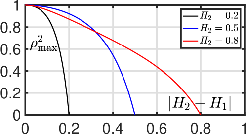
Figure 1: Interplay between the largest possible difference in selfsimilarity parameters and the largest (squared) correlation coefficients, for different $H_{2}$ (bivariate setting).

Finally, $B_{\Sigma,\underline{H}}\equiv{B}_{\Sigma,{\mathbf{W}}=\mathbb{I},\underline{H}}$ is obviously a special case of mfBm (cf., e.g., [21, 20, 19]). Yet, it displays no mixing across components, rendering the model less versatile for practical purposes.

III-C Wavelet analysis of mfBm

For mfBm, Eqs. (8) and (9) take the specific forms

$$\{D_{{B}_{\Sigma,{\mathbf{W}},\underline{H}}}(2^{j},k)\}_{k\in{\mathbb{Z}}}\stackrel{{\scriptstyle fdd}}{{=}}\left\{{\mathbf{W}}\,2^{j(\underline{H}+\frac{1}{2})}\,D_{{B}_{\Sigma,\underline{H}}}(2^{0},k)\right\}_{k\in{\mathbb{Z}}},$$ (17)

$$S_{{B}_{\Sigma,{\mathbf{W}},\underline{H}}}(2^{j})\stackrel{{\scriptstyle d}}{{=}}{\mathbf{W}}\,2^{j(\underline{H}+\frac{1}{2})}\,S_{{B}_{\Sigma,\underline{H}}}(2^{0})\,2^{j(\underline{H}+\frac{1}{2})}\,{\mathbf{W}}^{\top},$$ (18)

with $2^{j(\underline{H}+\frac{1}{2})}=\makebox{diag}(2^{j(H_{1}+1/2)},\ldots,2^{j(H_{M}+1/2)})$. This disentangles the contributions of the dilation vs. mixing operators to the shaping of the wavelet coefficients and spectrum.

Furthermore, Eqs. (10) and (11) obviously hold for mfBm. This permits to show, respectively, that both $\alpha_{k,k^{\prime}}^{m,m^{\prime}}$ and $\xi_{m}(2^{0})$ depend on $\mathbf{W}$ and $\Sigma$, but not on $\underline{H}$. An extension of the calculations in [25, 26] shows that $\xi_{m}(2^{0})$ actually depends only on the entries $\left(S_{{B}_{\Sigma,{\mathbf{W}},\underline{H}}}(2^{0})\right)_{(m^{{}^{\prime}},m^{{}^{\prime\prime}})}$ for $m\leq m^{\prime},m^{{}^{\prime\prime}}\leq M$ (see Remark .1 in Section -A of the supplementary material).

Finally and importantly, Eq. (11) demonstrates that the wavelet eigenvalue representations for both mfBm and ofBm disentangle the mixed power laws appearing in the wavelet spectrum $S_{{B}_{\Sigma,{\mathbf{W}},\underline{H}}}(2^{j})$. Thus, they restore the close relationship between power laws and scale-free dynamics, which had gotten altered by the mixing effect of the matrix ${\mathbf{W}}$. This motivates the estimation procedure $\underline{\hat{H}}^{\rm M}$ in Eq. (12), which thus applies to mfBm as well as to ofBm.

IV Selfsimilarity parameter vector estimation

IV-A Repulsion bias-corrected multivariate estimation

IV-A1 Repulsion bias

$\underline{\hat{H}}^{\rm M}$ in Eq. (12) is based on eigenvalues computed from the wavelet spectra $S_{{\cal B}_{\underline{\underline{H}},A}}(2^{j})$, namely, on the empirical wavelet coefficient covariance matrices estimated at different scales. However, it is well known that, for finite-size sample estimation of covariance matrices, eigenvalues undergo the so-called repulsion effect: Estimated eigenvalues tend to be farther apart one from the others, compared to true eigenvalues, all the more as the sample size is decreasing compared to the number of components (cf. e.g., [29]).

In the wavelet spectrum representation, this repulsion effect is enhanced by the fact that empirical wavelet coefficient covariance matrices are estimated with sample size $n_{j}$ that depends on analysis scales $2^{j}$, essentially as $n_{j}=2^{-j}N$. This induces scale-dependent repulsion biases in $\hat{\lambda}_{m}(2^{j})$, and hence an overall bias in $\underline{\hat{H}}^{\rm M}$ [27]. The repulsion bias is illustrated in Fig. 2 (left), which displays $\log_{2}\hat{\lambda}_{m}(2^{j})$ vs $\log_{2}2^{j}=j$. It is based on a synthetic mfBm with $M=6$ components of size $N=2^{12}$, with $H_{1}=\ldots=H_{6}=0.6$, a randomly selected orthonormal mixing matrix ${\mathbf{W}}\neq\mathbb{I}$ and a correlation matrix $\Sigma$ with off-diagonal coefficients set to $0.8$. The five smallest curves should thus theoretically superimpose, whereas discrepancies of amplitudes in estimated eigenvalues, increasing with scales, can be observed.

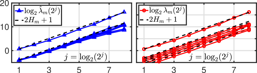
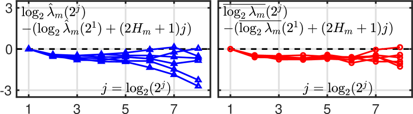
Figure 2: Repulsion bias in eigenvalue estimation. Top: Logarithms of estimated eigenvalues $\log_{2}\hat{\lambda}_{m}(2^{j})$ (left, blue) and $\overline{\log_{2}\lambda_{m}}(2^{j})$ (right, red), as functions of the logarithms of the scales $\log_{2}2^{j}=j$ for a synthetic mfBm with $M=6$, $N=2^{12}$, $\Sigma\neq\mathbb{I}$, ${\mathbf{W}}\neq\mathbb{I}$ and $H_{1}=\ldots=H_{6}=0.6$, and $j_{2}=8$. Superimposed straight lines indicate the theoretical slopes $2H_{m}+1$ (top, black). Bottom: Logarithms of estimated eigenvalues $\log_{2}\hat{\lambda}_{m}(2^{j})$ (left, blue) and $\overline{\log_{2}\lambda_{m}}(2^{j})$ (right, red) with theoretical linear behaviors subtracted.

IV-A2 Repulsion bias correction

Elaborating on [27], a novel estimation procedure for the estimation of $\underline{H}$ is devised and studied, hereinafter referred to as the bias-corrected estimator $\underline{\hat{H}}^{\rm M,bc}=(\hat{H}_{1}^{\rm M,bc},\ldots,\hat{H}_{M}^{\rm M,bc})$. The main idea behind its construction lies in using the same number of wavelet coefficients in the wavelet spectrum estimation at each scale. As a result, the eigenvalues computed from the wavelet spectra at different scales $2^{j}$ undergo an equivalent strength repulsion effect, i.e., one that does not vary with the scale $2^{j}$. To that end, let $2^{j_{2}}$ denote the largest analysis scale used in estimation (cf. Eq. (12)) and let $n_{j_{2}}$ be the number of corresponding wavelet coefficients at that scale. At each scale $2^{j_{1}}\leq 2^{j}\leq 2^{j_{2}}$, a collection of wavelet spectra are computed from $\tau=1,\ldots,2^{j_{2}-j}$ consecutive non-overlapping windows of wavelet coefficients with same size $n_{j_{2}}$:

$$S^{(\tau)}(2^{j}):=\frac{1}{n_{j_{2}}}\sum^{\tau n_{j_{2}}}_{k=1+(\tau-1)n_{j_{2}}}D_{{\cal B}_{\underline{\underline{H}},A}}(2^{j},k)D_{{\cal B}_{\underline{\underline{H}},A}}(2^{j},k)^{T}.$$ (19)

At each scale, the logarithms of the eigenvalues $\hat{\lambda}_{m}^{(\tau)}(2^{j})$ computed from each wavelet spectrum $S^{(\tau)}(2^{j})$ are then averaged across windows:

$$\overline{\log_{2}\lambda_{m}}(2^{j}):=2^{j-j_{2}}\sum_{\tau=1}^{2^{j_{2}-j}}\log_{2}\hat{\lambda}_{m}^{(\tau)}(2^{j}).$$ (20)

The impact of this bias correction procedure on the scaling of the eigenvalues is illustrated in Fig. 2 (right), which clearly shows that the theoretical slopes $2H_{m}+1$ are much better reproduced by the $\overline{\log_{2}\lambda_{m}}(2^{j})$ than by the classical $\log_{2}\hat{\lambda}_{m}(2^{j})$. The bias-corrected multivariate estimates $\hat{H}_{m}^{\rm M,bc}$ are thus defined as linear regressions across (the logarithms of the) scales $2^{j}$ of the averaged log-eigenvalues $\overline{\log_{2}\lambda_{m}}(2^{j})$:

$$\hat{H}_{m}^{\rm M,bc}=\frac{1}{2}\left(\sum_{j=j_{1}}^{j_{2}}w_{j}\overline{\log_{2}\lambda_{m}}(2^{j})-1\right).$$ (21)

The asymptotic estimation performance is studied theoretically in Section IV-B. The finite-size estimation performance is investigated numerically in Section V.

IV-A3 Nonmixing case

In the nonmixing case, i.e., when ${\mathbf{W}}=\mathbb{I}$, the selfsimilarity matrix reduces to $\underline{\underline{H}}=\mathrm{diag}(\underline{H})$. While the multivariate estimators $\hat{H}_{m}^{\rm M}$ in Eq. (12) and $\hat{H}_{m}^{\rm M,bc}$ in Eq. (21) obviously apply to the nonmixing case, a natural estimation procedure, extending univariate analysis, consists in performing linear regressions on the logarithms of the diagonal coefficients $S_{m,m}(2^{j})$ only:

$$\hat{H}_{m}^{\rm U}=\frac{1}{2}\left(\sum_{j=j_{1}}^{j_{2}}w_{j}\log_{2}S_{m,m}(2^{j})-1\right).$$ (22)

The resulting estimators $\hat{H}_{m}^{\rm U}$, intrinsically univariate in spirit, were intensively studied in [19] for nonmixing mfBm.

IV-B Theoretical study of asymptotic estimation performance

IV-B1 Asymptotic framework

The estimation performance is studied theoretically in the asymptotic double and joint limits of large sample sizes $N\rightarrow+\infty$, with linear regressions performed at coarse scales, in the range $(j_{1}(N),j_{2}(N))\rightarrow+\infty$. Technically, the scaling range is defined as $(j_{1}(N)=j_{1}^{0}+\log_{2}a(N),j_{2}(N)=j_{2}^{0}+\log_{2}a(N))$, where $(j_{1}^{0},j_{2}^{0})$ is an arbitrarily chosen range for $N_{0}$, and where $a(N)$ must satisfy:

$$a(N)2^{j_{2}}\leq N,\quad\frac{a(N)}{N}+\frac{N}{a(N)^{2\varpi+1}}\longrightarrow 0,\textrm{ as }N\rightarrow\infty,$$ (23)

$$\varpi=\min\left\{\min_{\{2\leq i\leq M|\;H_{i}-H_{i-1}>0\}}(H_{i}-H_{i-1}),\frac{H_{1}}{2}+\frac{1}{4}\right\}.$$ (24)

This essentially implies that $\log_{2}a(N)$ increases as $\beta\log_{2}N$, with $1/(2\varpi+1)<\beta<1$. This also implies that the number of scales involved in linear regressions does not vary with sample size $N$: $j_{2}(N)-j_{1}(N)+1=j_{2}^{0}-j_{1}^{0}+1$.

IV-B2 Asymptotic consistency

Theorem IV.1 establishes the asymptotic consistency of the bias-corrected estimator $\underline{\hat{H}}^{\rm M,bc}$:

Theorem IV.1.

Under Assumptions (OFBM1$-$3) and for a mother wavelet as defined in Section II-B1, (with $\stackrel{{\scriptstyle{\mathbb{P}}}}{{\rightarrow}}$ the convergence in probability):

1. For any $j=j_{1}^{0},\ldots,j_{2}^{0}$, $\tau=1,\ldots,2^{j_{2}^{0}-j}$ and $m=1,\ldots,M$, as $N\rightarrow\infty$,

   $$\frac{\hat{\lambda}_{m}^{(\tau)}(a(N)2^{j})}{a(N)^{2H_{m}+1}}\stackrel{{\scriptstyle{\mathbb{P}}}}{{\rightarrow}}\xi_{m}(2^{j})=(2^{j})^{2H_{m}+1}\xi_{m}(2^{0})>0,$$ (25)

   where $\hat{\lambda}^{(\tau)}_{1}(a(N)2^{j}),\ldots,\hat{\lambda}^{(\tau)}_{M}(a(N)2^{j})$ are the eigenvalues of $S^{(\tau)}(a(N)2^{j})$. Likewise, as $N\rightarrow\infty$,

   $$\frac{\lambda^{(\tau)}_{m}(a(N)2^{j})}{a(N)^{2H_{m}+1}}\rightarrow\xi_{m}(2^{j})=(2^{j})^{2H_{m}+1}\xi_{m}(2^{0})>0,$$ (26)

   where $\lambda^{(\tau)}_{1}(a(N)2^{j}),\ldots,\lambda^{(\tau)}_{M}(a(N)2^{j})$ are the eigenvalues of ${\mathbb{E}}S^{(\tau)}(a(N)2^{j})$.

2. Let $a(N)$ be as in (23). Then, as $N\rightarrow\infty$,

   $$\hat{H}^{\rm M,bc}_{m}\stackrel{{\scriptstyle{\mathbb{P}}}}{{\rightarrow}}H_{m},\quad\forall m=1,\ldots,M,$$ (27)

Proof.

For (i), the proof follows from adapting the technique for establishing Theorem 3.1 in [30], see Section -A of the supplementary material for details.

For (ii), Eq. (25) leads to the following equivalence:

$$\hat{H}^{\rm M,bc}_{m} =\frac{1}{2}\sum^{j_{2}^{0}}_{j=j_{1}^{0}}\frac{w_{j}}{2^{j_{2}^{0}-j}}\sum^{2^{j_{2}^{0}-j}}_{\tau=1}\Big{(}\log_{2}\frac{\hat{\lambda}^{(\tau)}_{m}(a(N)2^{j})}{a(N)^{2H_{m}+1}}$$ (28)

$$\qquad\qquad-\log_{2}a(N)^{2H_{m}+1}\Big{)}-\frac{1}{2}$$

$$\stackrel{{\scriptstyle{\mathbb{P}}}}{{\sim}}\frac{1}{2}\sum^{j_{2}^{0}}_{j=j_{1}^{0}}\frac{w_{j}}{2^{j_{2}^{0}-j}}\sum^{2^{j_{2}^{0}-j}}_{\tau=1}\Big{(}\log_{2}(2^{j})^{2H_{m}+1}\xi_{m}(2^{0})$$

$$\qquad\qquad-\log_{2}a(N)^{2H_{m}+1}\Big{)}-\frac{1}{2}$$

$$\stackrel{{\scriptstyle{\mathbb{P}}}}{{\sim}}\frac{1}{2}\sum^{j_{2}^{0}}_{j=j_{1}^{0}}w_{j}\Big{(}(2H_{m}+1)j+\log_{2}\frac{\xi_{m}(2^{0})}{a(N)^{2H_{m}+1}}\Big{)}-\frac{1}{2}.$$

Hence, by the definition of $w_{j}$, as $N\rightarrow\infty$,

$$\hat{H}^{\rm M,bc}_{m}\stackrel{{\scriptstyle{\mathbb{P}}}}{{\sim}}\frac{1}{2}[(2H_{m}+1)]-\frac{1}{2}=H_{m}.$$ (29)

This establishes (27). ∎

IV-B3 Simple eigenvalues condition

Our theoretical study of the asymptotic distribution relies on the condition that, asymptotically, all wavelet spectra eigenvalues are simple.
Condition (C0): $\forall m_{1},m_{2}\in\{1,\ldots,M\}$, with $m_{1}\neq m_{2}$,

$$H_{m_{1}}=H_{m_{2}}\Rightarrow\xi_{m_{1}}(2^{0})\neq\xi_{m_{2}}(2^{0}),$$ (30)

which states that either the selfsimilarity parameters $H_{m}$ are different, or when they are equal, $H_{m_{1}}=H_{m_{2}}$, $m_{1}\neq m_{2}$, the constants $\xi_{m}(2^{0})$ in Eq. (11) are different.

IV-B4 Asymptotic normality

Theorem IV.2 establishes the asymptotic normality of the bias-corrected estimator $\underline{\hat{H}}^{\rm M,bc}$:

Theorem IV.2.

Let $n_{a,j}=\frac{N}{a(N)2^{j}}$, $j=j^{0}_{1},\ldots,j^{0}_{2},$ be the number of wavelet coefficients available at scale $a(N)2^{j}$. Under Assumptions (OFBM1$-$3), for a mother wavelet as defined in Section II-B1, and assuming that (C0) holds, with $a(N)$ defined in (23) and where $\stackrel{{\scriptstyle d}}{{\rightarrow}}$ denotes the convergence in distribution:

1. Then, as $N\rightarrow\infty$,

   $$\left\{\sqrt{n_{a,j_{2}^{0}}}\big{(}\log_{2}\right. \left.\hat{\lambda}_{m}^{(\tau)}(a(N)2^{j})\right.$$ (31)

   $$\left.-\log_{2}\right.\left.\lambda_{m}^{(\tau)}(a(N)2^{j})\big{)}\right\}^{j=j_{1}^{0},\ldots,j_{2}^{0}}_{\begin{subarray}{c}\vspace{3mm}\\ m=1,\ldots,M\hfill\\ \tau=1,\ldots,2^{(j_{2}^{0}-j_{1}^{0})-j}\end{subarray}}$$

   $$\stackrel{{\scriptstyle d}}{{\rightarrow}}{\mathcal{N}}({\mathbf{0}},\Upsilon_{\bf B}),$$

   where $\Upsilon_{B}$ is a symmetric positive semidefinite matrix.

2. Moreover, as $N\rightarrow\infty$,

   $$\Big{\{}\sqrt{N/a(N)}\hskip 1.42262pt\big{(}\hat{H}^{\rm M,bc}_{m}-H_{m}\big{)}\Big{\}}_{m=1,\ldots,M}\stackrel{{\scriptstyle d}}{{\rightarrow}}{\mathcal{N}}({\mathbf{0}},\Sigma_{\bf B}),$$ (32)

   for some $\Sigma_{\bf B}\in{\mathcal{S}}_{\geq 0}(M,\mathbb{R})$.

Proof.

The proof follows from adapting the proof of asymptotic normality for the non bias-corrected multivariate estimator $\underline{\hat{H}}^{\rm M}$ from Theorem 3.2 in [30], as detailed in Section -B of the supplementary material. ∎

V Empirical finite-size estimation performance

The goal of the present section is to complement the theoretical study of estimation performance in the limit of large scales and large sample sizes. We do so by investigating their finite sample size counterparts by means of Monte Carlo simulations, conducted on synthetic mfBm. Different parametric configurations $(\Sigma,{\mathbf{W}},\underline{H})$ are used so as to further assess their impact on estimation performance.

The performance of the proposed bias-corrected multivariate estimator $\underline{\hat{H}}^{\rm M,bc}$ (Eq. (21)) is compared, in terms of biases, variances, Mean Squared Error (MSE), and covariance structures, to those of the multivariate estimator $\underline{\hat{H}}^{\rm M}$ (Eq. (12)) and of the univariate estimator $\underline{\hat{H}}^{\rm U}$ (Eq. (22)).

V-A Numerical simulation set-up

The Monte Carlo simulations involve $N_{\rm MC}=1000$ independent realizations of synthetic mfBm. The increments $\{B_{\Sigma,{\mathbf{W}},\underline{H}}(t+1)-B_{\Sigma,{\mathbf{W}},\underline{H}}(t)\}_{t=1,\ldots,N}$ of a mfBm, referred to as multivariate fractional Gaussian noise, form a multivariate stationary Gaussian process with covariance directly stemming from Eq. (14). Thus, it can be synthesized numerically by circulant embedding, cf. e.g., [31].

Results reported here are restricted to $M=6$ for the sake of clarity ; additional results for $M=20$, available upon request, led to identical conclusions. The range of sample sizes covered is $N\in\{2^{13},\ldots,2^{18}\}$. The parameters $\Sigma$, ${\mathbf{W}}$ and $\underline{H}$ are chosen to investigate a set of representative configurations:
Config1 ($\Sigma\neq\mathbb{I}$, ${\mathbf{W}}\neq\mathbb{I}$, $H_{m}$ all different) This corresponds to a generic situation involving mixing, nonzero correlations amongst components, as well as different selfsimilarity parameters. This type of situation calls for multivariate estimators ($\underline{\hat{H}}^{\rm M,bc}$, $\underline{\hat{H}}^{\rm M}$ ) ;
Config2 ($\Sigma\neq\mathbb{I}$, ${\mathbf{W}}\neq\mathbb{I}$, $H_{m}$ all equal) This corresponds to a generic situation with mixing and correlations amongst components. Yet, all selfsimilarity parameters are assumed equal. Thus, univariate estimation $\underline{\hat{H}}^{\rm U}$ could be used in this multivariate setting, as much as the $\underline{\hat{H}}^{\rm M,bc}$, $\underline{\hat{H}}^{\rm M}$ ;
Config3 ($\Sigma\neq\mathbb{I}$, ${\mathbf{W}}=\mathbb{I}$, $H_{m}$ all different) This corresponds to nonmixing instances. Hence, univariate $\underline{\hat{H}}^{\rm U}$ and multivariate estimation ($\underline{\hat{H}}^{\rm M,bc},\underline{\hat{H}}^{\rm M}$) are all legitimate procedures ;
Config4 ($\Sigma\neq\mathbb{I}$, ${\mathbf{W}}=\mathbb{I}$, $H_{m}$ all equal) This corresponds to nonmixing situations. Yet, all selfsimilarity parameters are equal, and thus both univariate $\underline{\hat{H}}^{\rm U}$ and multivariate estimations ($\underline{\hat{H}}^{\rm M,bc},\underline{\hat{H}}^{\rm M}$) should be appropriate procedures.
Config5 ($\Sigma=\mathbb{I}$, ${\mathbf{W}}\neq\mathbb{I}$, $H_{m}$ all different) This corresponds to mixing situations with different selfsimilarity parameters, yet with no correlation amongst fBms.

A generic covariance matrix $\Sigma$ is chosen: $\Sigma_{m,m^{\prime}}=0.7^{|m-m^{\prime}|}$, $1\leq m\leq m^{\prime}\leq M$. A mixing matrix ${\mathbf{W}}$ is randomly drawn from the set of $M\times M$ real-valued non-orthogonal matrices and kept fixed for all experiments. The selfsimilarity parameter vector $\underline{H}=(H_{1},\ldots,H_{6})$ is either set to $H_{m}=0.7$, $\forall m$, or $\underline{H}=(0.4,0.5,0.6,0.65,0.7,0.8)$. These different parameter configurations are chosen so that Condition (C0) holds – this condition is required for asymptotic normality claims (cf. Section IV-B3).

Wavelet analysis is performed using the least asymmetric Daubechies2 mother wavelet, with $N_{\psi}=2$ vanishing moments [28]. Linear regressions are performed, with $w_{j}$ as defined in [19], over scales that depend on the sample size $N$, as analyzed theoretically in Section IV-B1. Namely, we pick $2^{j_{1}}=a(N)2^{6}$ to $2^{j_{2}}=a(N)2^{9}$, where $a(N)=2^{\lfloor\beta\log_{2}(N/N_{0})\rfloor}$ with $\beta=0.9$ and $N_{0}=2^{13}$ (cf. Eq. (23)).

V-B Asymptotic normality assessment

The normality of $\underline{\hat{H}}^{\rm M,bc}$ is assessed by computing quantile-quantile plots for the squared Mahalanobis distance statistic

$$(\underline{\hat{H}}^{\rm M,bc}-{\mathbb{E}}\underline{\hat{H}}^{\rm M,bc})\mathrm{Var}(\underline{\hat{H}}^{\rm M,bc})^{-1}\;(\underline{\hat{H}}^{\rm M,bc}-{\mathbb{E}}\underline{\hat{H}}^{\rm M,bc})^{\top}.$$ (33)

In (33), the ensemble average $\mathbb{E}$ is practically computed as the mean across independent realizations. Samples of the random variable (33) are plotted against a $\chi^{2}$ distribution with $M$ degrees of freedom, since this distribution is expected to hold under the exact joint normality of $\underline{\hat{H}}^{\rm M,bc}$. Fig. 3 reports such quantile-quantile plots, for the different configurations and for different sample sizes. It shows very satisfactory straight lines, even at the smallest sample size $N=2^{13}$. This suggests that the joint normality for $\underline{\hat{H}}^{\rm M,bc}$ holds very satisfactorily for finite sample size estimation, even for small sample sizes. It thus indicates fast convergence to asymptotic normality, proven theoretically in Theorem IV.2 (Eq. (32)).

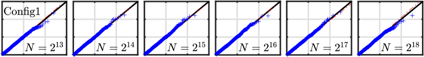
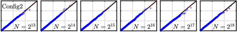
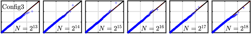
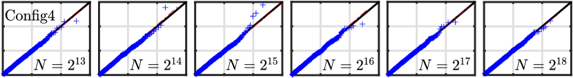
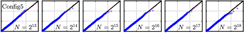
Figure 3: Finite-size joint normality for $\bm{\underline{\hat{H}}^{\rm M,bc}}$. Quantile-quantile plots of the empirical distribution of the Mahalanobis distance computed from the bias-corrected multivariate estimates $\underline{\hat{H}}^{\rm M,bc}$ against a $\chi^{2}$ distribution with $M$ degrees of freedom (expected theoretically under joint normality), for different sample sizes $N$ and different configurations.

V-C Estimation performance: bias, covariance, MSE

For any estimate of the vector of selfsimilarity parameters $\underline{\hat{H}}$, matrices of bias, covariance and MSE are defined as

$$\textrm{Bias}^{2}(\underline{\hat{H}}) =(\mathbb{E}\underline{\hat{H}}-\underline{H})(\mathbb{E}\underline{\hat{H}}-\underline{H})^{\top},$$ (34)

$$\textrm{Cov}(\underline{\hat{H}}) =\mathbb{E}\left[(\mathbb{E}\underline{\hat{H}}-\underline{\hat{H}})(\mathbb{E}\underline{\hat{H}}-\underline{\hat{H}})^{\top}\right],$$ (35)

$$\mathrm{MSE}(\underline{\hat{H}}) =\mathbb{E}\left[(\underline{\hat{H}}-\underline{H})(\underline{\hat{H}}-\underline{H})^{\top}\right].$$ (36)

The estimation performance is quantified by the spectral norm of these matrices, i.e., by the largest absolute value of their eigenvalues  [32].

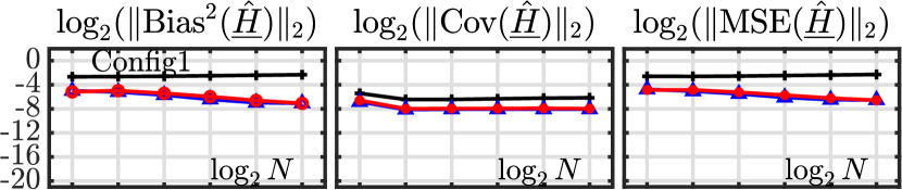
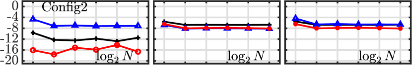
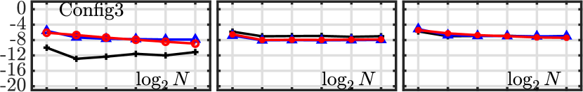
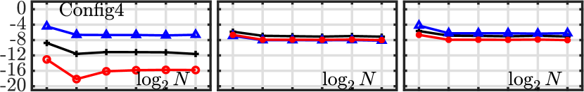
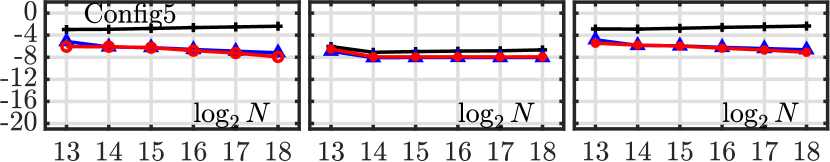
Figure 4: Estimation performance. Logarithm of the spectral norms of the bias (left), covariance (middle) and MSE (right) for the proposed bias-corrected multivariate estimator $\underline{\hat{H}}^{\rm M,bc}$ (red), compared to those for the classical multivariate estimator $\underline{\hat{H}}^{\rm M}$ (blue) and for the univariate estimator $\underline{\hat{H}}^{\rm U}$ (black), as functions of the logarithm of the sample size $N$.

Fig. 4 reports the (logarithms of the) spectral norms of the bias, covariance and MSE for the proposed bias-corrected multivariate estimator $\underline{\hat{H}}^{\rm M,bc}$, compared to those for the classical multivariate estimator $\underline{\hat{H}}^{\rm M}$ and for the univariate estimator $\underline{\hat{H}}^{\rm U}$. The results are shown as functions of the logarithm of the sample size $N$ and for each of the different configurations.

For the generic case represented by Config1 (Fig. 4, first row), the univariate estimator $\underline{\hat{H}}^{\rm U}$ suffers from significant bias stemming from the component mixing caused by ${\mathbf{W}}$. Thus, it is significantly outperformed by the multivariate estimators $\underline{\hat{H}}^{\rm M}$ and $\underline{\hat{H}}^{\rm M,bc}$. The latter show equivalent performance as the combination of $\Sigma$, ${\mathbf{W}}$ and different $H_{m}$ yield different eigenvalues for $\mathbb{E}S(2^{j})$ at all scales and thus small repulsion bias in their estimated values.

For Config2 (Fig. 4, second row), with mixing yet equal $H_{m}$, the eigenvalues of $\mathbb{E}S(2^{j})$ lie much closer to each other at most scales and hence suffer from substantial repulsion biases in their estimation. This results in a significant bias for the classical multivariate estimator $\underline{\hat{H}}^{\rm M}$. Fig. 4, middle row, shows that the proposed bias-corrected multivariate estimator $\underline{\hat{H}}^{\rm M,bc}$ succeeds in significantly reducing bias without an increase in the variance. This leads to an overall much improved estimation performance as quantified by the MSE. While the univariate estimator $\underline{\hat{H}}^{\rm U}$ displays small bias, as expected in view of the equality of all selfsimilarity parameters, it also shows greater variance, thus, greater MSE, when compared to the proposed $\underline{\hat{H}}^{\rm M,bc}$.

For the nonmixing case, Config3 (Fig. 4, third row), the univariate estimator $\underline{\hat{H}}^{\rm U}$ naturally shows much smaller biases compared to the multivariate estimators $\underline{\hat{H}}^{\rm M}$ and $\underline{\hat{H}}^{\rm M,bc}$. Yet, it also displays larger variances. Thus, as a result of bias-variance trade-off, the MSE of all three estimators are equivalent. Importantly, this shows that even for data corresponding to nonmixing situations, there is no cost in estimation performance associated with the use of multivariate estimators.

For the nonmixing case with equal $H_{m}$, Config4 (Fig. 4, fourth row), the univariate estimator $\underline{\hat{H}}^{\rm U}$ and bias-corrected multivariate estimator $\underline{\hat{H}}^{\rm M,bc}$ perform similarly to Config2. This suggests that, for $H_{m}$ all equal, the presence of mixing has no impact in terms of bias or variance. However, estimation performance of the multivariate estimator $\underline{\hat{H}}^{\rm M}$ is slightly more affected than in Config2, showing that the repulsion bias is more substantial in the absence of mixing.

Finally, for the mixing case with different $H_{m}$ and no correlation, Config5 (Fig. 4, fifth row), the performances are similar to those for Config1 for all three estimators, indicating their robustness against component correlations $\Sigma$.

All together, the results reported in Fig. 4 lead us to conclude that the proposed bias-corrected multivariate estimator $\underline{\hat{H}}^{\rm M,bc}$ displays the best estimation performance regardless of the actual configuration of the parameters. In practice it is not a priori known whether or not mixing is present, or whether selfsimilarity parameters are pairwise distinct or equal. We have seen that the estimator $\underline{\hat{H}}^{\rm U}$ fails when mixing is present. Also, we have found out that the estimator $\underline{\hat{H}}^{\rm M}$ fails when repulsion bias is present, i.e., when one needs to estimate identical selfsimilarity parameters. By contrast, $\underline{\hat{H}}^{\rm M,bc}$ displays neither one of these limitations – this versatility is clearly an important property that motivates its practical use.

V-D Covariance structure of $\underline{\hat{H}}^{\rm M,bc}$

V-D1 Correlation structure

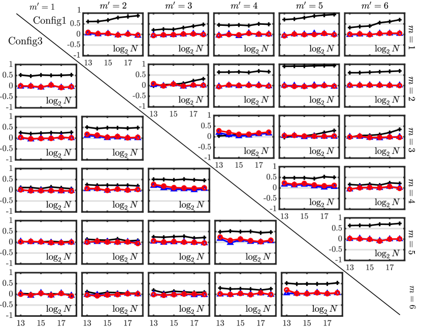
Figure 5: Correlation structures of $\bm{\underline{\hat{H}}^{\rm M,bc}}$, $\bm{\underline{\hat{H}}^{\rm M}}$ and $\bm{\underline{\hat{H}}^{\rm U}}$. Correlation coefficients between entries $\hat{H}_{m}$ and $\hat{H}_{m^{\prime}}$, $1\leq m\neq m^{\prime}\leq M$, for $\underline{\hat{H}}^{\rm M,bc}$ (red), $\underline{\hat{H}}^{\rm M}$ (blue) and $\underline{\hat{H}}^{\rm U}$ (black), as functions of sample sizes $N$, for Config1 (upper right triangle) and Config3 (lower left triangle) .

We complement the estimation performance assessment by turning to the dependence structure amongst estimates – the latter constitutes a key feature in the practical use of the estimators of the selfsimilarity parameters. Asymptotic normality, as well as finite sample size approximate normality, hint on the importance of the correlation structure amongst estimated selfsimilarity parameters. Fig. 5 thus compares correlation coefficients between pairs $(\hat{H}_{m},\hat{H}_{m^{\prime}})$, $1\leq m<m^{\prime}\leq M$, as functions of the sample size $N$, for the three different estimators $\underline{\hat{H}}^{\rm M,bc}$, $\underline{\hat{H}}^{\rm M}$ and $\underline{\hat{H}}^{\rm U}$. The correlation structures are compared only for Config1 and Config3, in upper and lower triangles respectively. The conclusions drawn about the other configurations are similar.

Fig. 5 clearly indicates that most pairs $(\hat{H}^{\rm U}_{m},\hat{H}^{\rm U}_{m^{\prime}})$, $1\leq m<m^{\prime}\leq M$, remain significantly correlated, even for large sample sizes. By contrast, for the multivariate estimators, the pairs $(\hat{H}^{\rm M,bc}_{m},\hat{H}^{\rm M,bc}_{m^{\prime}})$ and $(\hat{H}^{\rm M}_{m},\hat{H}^{\rm M}_{m^{\prime}})$, $1\leq m<m^{\prime}\leq M$ are quasi-decorrelated, for all sample sizes. These observations partly explain why the overall contribution of the variance to the MSE was larger for the univariate estimators when compared to the multivariate estimators (cf. Fig. 4 above). These empirical observations are complemented and framed by the analytical calculations detailed in Sections -C and -D of the supplementary material. These show the following striking fact. Suppose Condition (C0) holds, and further assume that the weak correlation structure amongst wavelet coefficients of mfBm can be approximated into exact decorrelation. Then, the covariance matrices $\Sigma_{\bf B}$ in Eq. (31) and $\Upsilon_{\bf B}$ in Eq. (32) of Theorem IV.2 are well approximated, to the first order, by diagonal matrices. These empirical observations and analytical calculations reveal an important advantage of the mutivariate $\underline{\hat{H}}^{\rm M,bc}$ (and $\underline{\hat{H}}^{\rm M}$) against the univariate $\underline{\hat{H}}^{\rm U}$, even for nonmixing data: namely, that the former consist of asymptotically Gaussian, weakly dependent random vectors. This is a major practical feature, e.g., in the design of tests for the equality of selfsimilarity parameters, which is of significant interest in many applications [27, 33].

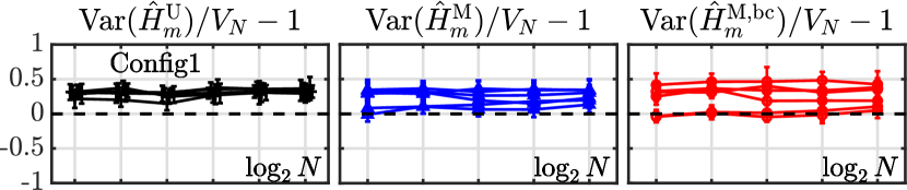
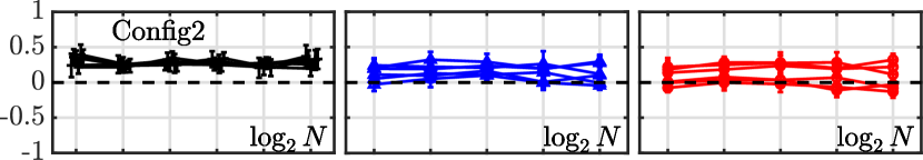
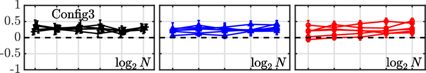
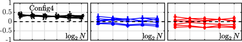
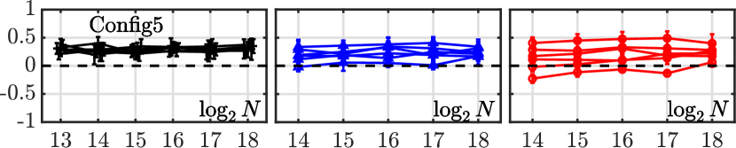
Figure 6: Approximation of the variance. Relative differences between empirical variances of the (left, black) univariate estimator $\hat{H}^{\rm U}_{m}$, (middle, blue) multivariate estimator $\hat{H}^{\rm M}_{m}$ and (right, red) bias-corrected multivariate estimator $\hat{H}^{\rm M,bc}_{m}$ and the approximate variance $V_{N}$ (Eq. (38)) with superimposed components $m=1,\ldots,6$ as functions of the sample size $N$.

V-D2 Variance

Besides approximate asymptotic decorrelation, the diagonal entries of the matrices $\Sigma_{\bf B}$ and $\Upsilon_{\bf B}$ remain to be discussed. The calculations reported in Remark .2 in Section -B, and in Sections -C and -D of the supplementary material show that these diagonal entries can be first-order approximated by a constant:

$$\Upsilon_{\bf B}\simeq 2\,{(\log_{2}e)^{2}}\,\mathbb{I}\makebox{ and }\Sigma_{\bf B}\simeq\frac{(\log_{2}e)^{2}}{2}\sum_{j=j_{1}^{0}}^{j_{2}^{0}}{w_{j}^{2}}{2^{j}}\,\,\mathbb{I}.$$ (37)

Specifically, this implies that, under the approximation of decorrelation between wavelet coefficients of mfBm and under (C0), the finite-size variances of $\hat{H}^{\rm M,bc}_{m}$ and $\hat{H}^{\rm M}_{m}$, for every $m\in\{1,\ldots,M\}$, can be approximated as:

$$\mathrm{Var}(\hat{H}^{\rm M,bc}_{m})\approx\mathrm{Var}(\hat{H}^{\rm M}_{m})\approx\displaystyle\frac{(\log_{2}e)^{2}}{2}\sum_{j=j_{1}}^{j_{2}}\frac{w_{j}^{2}}{n_{j}}:=V_{N}.$$ (38)

When $N\rightarrow+\infty$, one obviously has $(N/a(N))V_{N}\rightarrow$ $\frac{(\log_{2}e)^{2}}{2}\sum_{j=j_{1}^{0}}^{j_{2}^{0}}{w_{j}^{2}}{2^{j}}$. Thus, in conclusion, $\mathrm{Var}(\hat{H}^{\rm M}_{m})$ and $\mathrm{Var}(\hat{H}^{\rm M,bc}_{m})$ decrease with sample size $N$ and depend on the range of regressions scales $j_{1}$ and $j_{2}$. However, to the first order, these depend on none of the model parameters $\Sigma$, ${\mathbf{W}}$ and $\underline{H}$. This renders them comparable for all components. Interestingly, it was shown in  [19] that, for the univariate $\hat{H}^{\rm U}_{m}$ in nonmixing settings, the variance can be approximated to the first order by the same closed-form relation: $\mathrm{Var}(\hat{H}^{\rm U}_{m})\approx V_{N}$.

To further assess the practical relevance of the finite sample size approximation in Eq. 38, Fig. 6 reports the relative difference between the empirical variances of $\hat{H}^{\rm U}_{m}$, $\hat{H}^{\rm M}_{m}$ and $\hat{H}^{\rm M,bc}_{m}$ and $V_{N}$ as a function of the logarithm of the sample size $N$ for $m=1,\ldots,6$ and for the different configurations. Fig. 6 (left column), first, shows that, in all configurations, the variance of the univariate estimator $\hat{H}^{\rm U}_{m}$ is approximated by $V_{N}$ with a $20\%$ relative error resulting from the non-exact decorrelation of eigenvalues between scales. This first result extends the results reported in [19], limited to nonmixing cases. Fig. 6, second, confirms that the variances of the three estimators neither depend on $\underline{H}$ (Config1 vs. Config2), nor on ${\mathbf{W}}$ (Config1 vs. Config3), nor on $\Sigma$ (Config1 vs. Config5). Fig. 6, third, confirms that the variances of the multivariate estimators are, on average, lower than those of the univariate estimator. In summary, Fig. 6 shows that the closed-form approximation $V_{N}$ in Eq. (38) is valid in all configurations for the three estimators, even for small sample sizes. This constitutes a valuable result for practical use in applications e.g., when testing the equality of selfsimilarity parameters.

VI Application to epileptic seizure prediction

Selfsimilarity has been broadly used to model temporal dynamics in macroscopic brain activity. The purpose of the modeling effort is either to study healthy brain mechanisms (cf. e.g., [9, 34, 10]), or to diagnose brain disorders and pathologies. Notably, there is a particular interest in epileptic seizure prediction [35]. Yet, most studies have so far remained based on univariate analysis of scale-free dynamics, while brain dynamics is naturally conducive to multivariate analysis. The aim of this section is, thus, to comparatively assess the potential of multivariate and univariate selfsimilarity parameter estimations in the detection of preictal states (i.e., time periods prior to seizure onsets) against interictal states (i.e., periods distant in time from any seizure).

The multi-channel EEG recordings studied here were collected at the Boston Children’s Hospital from pediatric patients with medically intractable seizures, from the CHB-MIT Scalp EEG database [36], available at https://physionet.org/content/chbmit/1.0.0/. EEG recordings stem from the International 10-20 system of EEG electrode positions and nomenclature, last for at least one hour, and are sampled at 256Hz. Multivariate analyses are performed for the 19 channels, within sliding 2-minute long windows. Wavelet analysis is performed using the least asymmetric Daubechies2 mother wavelet.

Fig. 7 reports, for both interictal and preictal windows, the logarithms of the diagonal entries of the wavelet spectrum $S(2^{j})$, $\log_{2}S_{m,m}(2^{j})$, the log-eigenvalues $\log_{2}\hat{\lambda}_{m}(2^{j})$ and the proposed bias-corrected log-eigenvalues $\overline{\log_{2}\lambda_{m}}(2^{j})$, all of them as functions of scales $2^{j}$ for $m=1,\ldots,19$. Fig. 7 shows linear behaviors for these functions across fine scales $1\leq 2^{j}\leq 2^{7}$, that hence indicate scale-free dynamics in these EEG time series, at frequencies above $1$Hz, in agreement with the literature on epilepsy, cf. e.g., [37]. These scale-free dynamics hold for both preictal and interictal states, and both component-wise (univariate, $\log_{2}S_{m,m}(2^{j})$) and jointly (multivariate, $\log_{2}\hat{\lambda}_{m}(2^{j})$ and $\overline{\log_{2}\lambda_{m}}(2^{j})$). The observed multivariate selfsimilarity constitutes per se a significant outcome of this work as selfsimilarity in EEG time series had so far only been observed component per component and not jointly. Combined with literature suggesting that differences between preictal and interictal dynamics are related to frequencies ranging from $10$Hz to $85$Hz [37], these observations suggest performing linear regressions for the estimation of $\underline{H}$ across scales ranging from $2^{1}\leq 2^{j}\leq 2^{4}$.

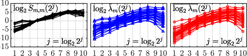
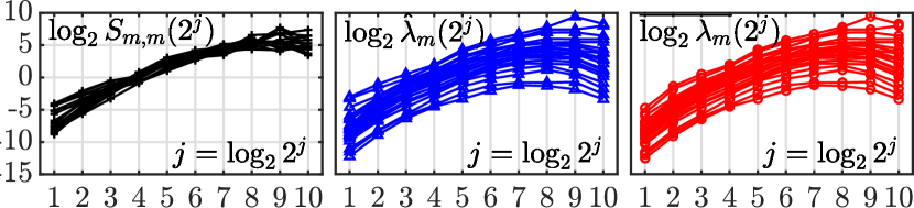
Figure 7: Multivariate scale-free dynamics in EEG time series, for preictal and interictal states. Logarithms of the estimated diagonal entries $\log_{2}S_{m,m}(2^{j})$ (left, black) , estimated eigenvalues $\log_{2}\hat{\lambda}_{m}(2^{j})$ (middle, blue) and bias corrected eigenvalues $\overline{\log_{2}\lambda_{m}}(2^{j})$ (right, red), of the wavelet spectrum, for $m=1,\ldots,19$, for interictal (top) and preictal (bottom) windows.

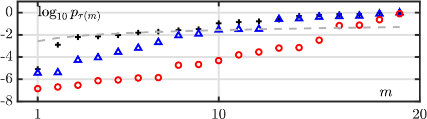
Figure 8: Differences in multivariate selfsimilarity between preictal and interictal states. Logarithms of the sorted p-values for Wilcoxon rank-sum tests between preictal and interictal distributions for univariate estimates $\hat{H}^{\rm U}_{m}$ (black), multivariate estimates $\hat{H}^{\rm M}_{m}$ (blue) and bias corrected multivariate estimates $\hat{H}^{\rm M,bc}_{m}$ (red), vs. Benjamini-Hochberg multiple hypothesis testing thresholds (grey dashed line).

Fig. 8 compares the (logarithms of) sorted Wilcoxon rank-sum test p-values $p_{\tau(m)}$ measuring the significance of the differences between the medians of preictal vs. interictal distributions, for the univariate estimator $\underline{\hat{H}}^{\rm U}$ (Eq. (22)), the multivariate estimator $\underline{\hat{H}}^{\rm M}$ (Eq. (12)) and the bias-corrected multivariate estimator $\underline{\hat{H}}^{\rm M,bc}$ (Eq. (21)). The p-values are ranked and compared to Benjamini-Hochberg multiple hypothesis thresholds [38], computed at a false discovery rate $\alpha=0.05$. For all three estimators, the medians of the distributions of estimated selfsimilarity parameters clearly differ from preictal to interictal states, thus indicating that the scale-free structure of the temporal dynamics is modified by forthcoming epileptic seizures. Moreover, the bias-corrected multivariate estimator $\underline{\hat{H}}^{\rm M,bc}$ shows stronger differences in selfsimilarity parameters between preictal and interictal states, compared to either the univariate estimates $\underline{\hat{H}}^{\rm U}$ or the multivariate estimates $\underline{\hat{H}}^{\rm M}$. This illustrates the benefits of both taking into account cross-temporal dynamics in EEG time series analysis and correcting the repulsion bias in multivariate estimation for epilepsy seizure prediction.

These analyses are reported for a single patient only (Patient $22$). Equivalent conclusions were drawn for all other patients. Of importance, the distributions of selfsimilarity parameters are found to differ significantly from one patient to another. This demands a single-patient procedure to detect preictal vs. interictal states. Interested readers are referred to the in-depth study carried out in [39].

VII Conclusion

In this work, we have, first, proposed a multivariate selfsimilarity model, defined as a linear mixture of correlated fractional Brownian motions, well-suited to adjust the versatility of real-world multivariate data, and formally related it to a former mathematical model. Second, we have turned the formal proposition of wavelet spectrum eigenvalue-based estimation for the vector of selfsimilarity parameters proposed in [25, 26], into a versatile and robust bias-corrected estimation procedure that can actually be used on real-world data. Its performance was studied mathematically in terms of asymptotics and by numerical simulations for finite-size samples. This permitted showing that the proposed multivariate estimators work in a broader context (mixing) than the univariate one and still performs better (decorrelation) in the nonmixing case, where the univariate estimator can be used. Third, its potential was illustrated at work on real multi-channel EEG data in a context of epileptic seizure prediction. A documented toolbox implementing estimation will be made publicly available at the time of publication.

Future investigations include incorporating a multivariate time-scale bootstrap procedure so as to assess confidence levels in estimation from a single realization of data. Also, large-dimensional asymptotics will be studied both theoretically and numerically to account for situations where the number of components grows as fast as sample size, of major practical importance in real-world applications.

Fix $\ell\in\mathbb{N}$. Throughout the appendices, ${\mathcal{S}}(\ell,\mathbb{R})$ and ${\mathcal{S}}_{\geq 0}(\ell,\mathbb{R})$ denote, respectively, the space of symmetric and the cone of symmetric positive semidefinite $\ell\times\ell$ matrices. The notation $\textnormal{vec}_{{\mathcal{S}}}$ denotes the projection on the free entries of a symmetric matrix. Also, $\pi_{i_{1},i_{2}}$ and $\pi_{i_{1},i_{2},\ldots,i_{\ell}}$, $\ell\in\mathbb{N}$, denote the projection of a matrix or vector, respectively, on its entries $i_{1},i_{2}$ and $i_{1},i_{2},\ldots,i_{\ell}$. We express any vector ${\mathbf{v}}$ entry-wise as $\{{\mathbf{v}}_{\ell}\}_{\ell}$. Recall that $n_{a,j}=\frac{N}{a(N)2^{j}}$, $j=j^{0}_{1},\ldots,j^{0}_{2}$.

-A Proof of consistency

Proof.

We only show $(i)$. Fix $j\in\{j_{1}^{0},\ldots,j_{2}^{0}\}$, $\tau\in\{1,\ldots,2^{j^{0}_{2}-j}\}$ and $m\in\{1,\ldots,M\}$. Suppose, for the moment, that the limit (25) holds. Recall that $\operatorname*{\mathit{p}-lim}_{N\rightarrow\infty}$ denotes limit in probability. Writing $\widetilde{a}(N)=a(N)2^{j}$,

$$\xi_{m}(2^{j}) =\operatorname*{\mathit{p}-lim}_{N\rightarrow\infty}\frac{\hat{\lambda}_{m}^{(\tau)}(a(N)2^{j})}{a(N)^{2H_{m}+1}}$$ (39)

$$=\operatorname*{\mathit{p}-lim}_{N\rightarrow\infty}\frac{\hat{\lambda}_{m}^{(\tau)}\big{(}\widetilde{a}(N)\big{)}}{(\widetilde{a}(N)2^{-j})^{2H_{m}+1}}$$

$$=2^{j(2H_{m}+1)}\xi_{m}(1).$$

This establishes the scaling relationship in (25).

We now need to show the convergence in (25). The argument follows from a simple adaptation of the technique for establishing Theorem 3.1 in [30], which originally pertains to a high-dimensional context.

In fact, in that theorem the measurements are given by a high-dimensional signal-plus-noise stochastic process of the form $Y(t)={\mathbf{P}}(N)X(t)+Z(t)$, where, for $p\geq M$, $Y(t),Z(t)\in\mathbb{R}^{p}$, ${\mathbf{P}}(N)\in{\mathcal{M}}(p,M,\mathbb{R})$ and $X(t)\in\mathbb{R}^{M}$. $X(t)$ is the latent fractional stochastic process (the “signal"), $Z(t)$ is the “noise" component, and ${\mathbf{P}}(N)$ is a full rank matrix of coordinates. So, first assume the dimension $p$ is fixed and set to $M$. Now suppose $X(t)$ is an ofBm under the conditions of Theorem IV.1. Next set the matrix ${\mathbf{P}}(N)$ to the $M\times M$ identity matrix. In addition, suppose the noise term $Z(t)$ is identically zero. In order to establish (25), it now suffices to follow the argument of the proof of Theorem 3.1 in  [30]. The convergence (26) can be established by an analogous argument. This shows $(i)$. ∎

Remark .1.

The framework for proving Theorem IV.1 provides a great deal of information about the asymptotic rescaled eigenvalues $\xi_{m}(2^{j})$, $m\in\{1,\ldots,M\}$, as in (25). More specifically, for some function $\varphi$ and some vector $\widetilde{{\mathbf{w}}}$, we can write

$$\operatorname*{\mathit{p}-lim}_{N\rightarrow\infty}\frac{\hat{\lambda}^{(\tau)}_{m}(a(N)2^{j})}{a(N)^{2H_{m}+1}}=\xi_{m}(2^{j})=\varphi(\widetilde{{\mathbf{w}}}).$$ (40)

In order to describe $\varphi(\widetilde{{\mathbf{w}}})$, we need a few definitions and constructs. So, for the fixed $m$, define the sets of indices $\mathcal{I}_{-}:=\{\ell:H_{\ell}<H_{m}\}$ and

$$\mathcal{I}_{0}:=\{\ell:H_{\ell}=H_{m}\}\textnormal{ {and} }\mathcal{I}_{+}:=\{\ell:H_{\ell}>H_{m}\}.$$ (41)

Note that $\mathcal{I}_{-}$ and $\mathcal{I}_{+}$ are possibly empty. Also, let

$$r_{1}:=\textnormal{card}(\mathcal{I}_{-}),\hskip 2.84526ptr_{2}:=\textnormal{card}(\mathcal{I}_{0})\geq 1,\hskip 2.84526ptr_{3}:=\textnormal{card}(\mathcal{I}_{+})$$ (42)

be their respective cardinalities. For every $\tau=1,\ldots,2^{j^{0}_{2}-j}$, define the auxiliary wavelet random matrix

$$\mathbf{\widehat{B}}^{(\tau)}_{a}(2^{j}):={\mathbf{W}}^{-1}a^{-\underline{\underline{H}}-\frac{1}{2}\mathbb{I}}{S}^{(\tau)}\big{(}a2^{j}\big{)}a^{-\underline{\underline{H}}^{*}-\frac{1}{2}\mathbb{I}}({\mathbf{W}}^{*})^{-1},$$ (43)

where $a\equiv a(N)$. Also, let $\mathbf{B}(2^{j})={\mathbb{E}}\mathbf{B}_{a}(2^{j})$, which neither depends on $\tau$ nor on $a$. Recast

$$\widehat{\mathbf{B}}^{(\tau)}_{a}(2^{j})=(\widehat{\mathbf{B}}_{i\ell})_{i,\ell=1,2,3},\quad{\mathbf{B}}(2^{j})=(\mathbf{B}_{i\ell})_{i,\ell=1,2,3}.$$ (44)

In (44), ${\mathbf{B}}_{i\ell}$ and $\widehat{\mathbf{B}}_{i\ell}$ denote blocks of size $r_{i}\times r_{\ell}$, and the scale $2^{j}$ is omitted wherever doing so is unambiguous. Similarly, define

$$\mathbf{W}=\big{(}\mathbf{W}_{1}~{}\mathbf{W}_{2}~{}\mathbf{W}_{3}\big{)},$$ (45)

where, for $i=1,2,3$, $\mathbf{W}_{i}\in{\mathcal{M}}(p,r_{i},\mathbb{R})$, and each column vector is denoted by $\mathbf{w}_{\ell}$, $\ell=1,\ldots,r$. Let ${\bm{\Pi}}_{3}\in{\mathcal{M}}(r,\mathbb{R})$ be the projection matrix onto $\textnormal{Ker}\{{\mathbf{W}}^{*}_{3}\}$. Also, let ${\mathbf{M}}={\mathbf{B}}_{22}-{\mathbf{B}}_{23}{\mathbf{B}}^{-1}_{33}{\mathbf{B}}_{32}\in{\mathcal{S}}(r_{2},\mathbb{R})$ and ${\bm{\Lambda}}={\bm{\Pi}}^{*}_{3}{\mathbf{W}}_{2}{\mathbf{M}}{\mathbf{W}}^{*}_{2}{\bm{\Pi}}_{3}\in{\mathcal{S}}_{\geq 0}(r,\mathbb{R})$. For unit vectors ${\mathbf{u}}\in\mathbb{R}^{r}$, define the function

$$\varphi({\mathbf{u}}):={\mathbf{u}}^{*}{\bm{\Lambda}}{\mathbf{u}}.$$ (46)

Then, for $\varphi$ as in (46), the proof of Proposition 5.1 and Lemma B.1 in [30] imply that there exists a possibly random vector

$$\widetilde{{\mathbf{w}}}=\widetilde{{\mathbf{w}}}(\omega)\in\textnormal{span}\{{\bm{\Lambda}}\}=\textnormal{span}\{{\mathbf{W}}_{2},{\mathbf{W}}_{3}\}\cap\textnormal{Ker}\{{\mathbf{W}}^{*}_{3}\}$$ (47)

based on which we can express the limit (40) as $\varphi(\widetilde{{\mathbf{w}}})$ (n.b.: $\xi_{m}(2^{j})$ is deterministic). In particular, relations (46) and (47) imply that $\varphi({\mathbf{w}})$ – and, hence, $\xi_{m}(2^{j})$ – only depends on the matrices ${\mathbf{B}}_{22}$, ${\mathbf{B}}_{23}$, ${\mathbf{B}}_{33}$, ${\mathbf{W}}_{2}$ and ${\mathbf{W}}_{3}$. Consequently, the asymptotic rescaled function in (25) only depends on parameters associated with the index sets ${\mathcal{I}}_{0}$ and ${\mathcal{I}}_{+}$ in (41).

-B Proof of asymptotic normality

In the proof of Theorem IV.2, we write $a\equiv a(N)$ whenever notationally convenient. Also, we make use of the following notation. Let $\{X_{N}\}_{N\in\mathbb{N}}$, $\{Y_{N}\}_{N\in\mathbb{N}}$ be two sequences of random variables. We write $X_{N}\stackrel{{\scriptstyle d}}{{\sim}}Y_{N}$, $N\rightarrow\infty$, when the two sequences have the same limit in distribution, which is assumed to be well defined.

Proof.

First, we show $(i)$. Fix $j\in\{j^{0}_{1},\ldots,j^{0}_{2}\}$. The proof of (31) is by means of an adaptation of the proof of Theorem 3.2 in [30]. In fact, let $\widehat{\mathbf{B}}_{a}(2^{j})$ and ${\mathbf{B}}(2^{j})$ be as in (44). Under conditions (OFBM1-3), as a consequence of Theorem 3.1 in [25],

$$\Big{\{}\sqrt{n_{a,j^{0}_{2}}}\hskip 1.42262pt\textnormal{vec}_{{\mathcal{S}}}\big{(}\mathbf{\widehat{B}}^{(\tau)}_{a}(2^{j})-\mathbf{B}(2^{j})\big{)}\Big{\}}_{\tau=1,\ldots,2^{j^{0}_{2}-j}}\stackrel{{\scriptstyle d}}{{\rightarrow}}{\mathcal{N}}(0,\Sigma_{\mathbf{B}})$$ (48)

as $n\rightarrow\infty$ for some $\Sigma_{\mathbf{B}}\in{\mathcal{S}}_{\geq 0}\big{(}2^{j^{0}_{2}-j}\cdot M(M+1)/2,\mathbb{R}\big{)}$. In particular,

$$\mathbf{\widehat{B}}^{(\tau)}_{a}(2^{j})-\mathbf{B}(2^{j})\stackrel{{\scriptstyle{\mathbb{P}}}}{{\rightarrow}}0,\quad\tau=1,\ldots,2^{j^{0}_{2}-j}.$$ (49)

So, fix $m\in\{1,\ldots,M\}$. Recall that, for any matrix $\mathds{M}\in{\mathcal{S}}(M,\mathbb{R})$, the differential of a simple eigenvalue $\lambda_{m}(\mathds{M})$ exists in a connected vicinity of $\mathds{M}$ and is given by

$$d\lambda_{m}(\mathds{M})=\mathbf{u}^{*}_{m}\{d\hskip 0.7113pt\mathds{M}\}\mathbf{u}_{m},$$ (50)

where $\mathbf{u}_{m}$ is a unit eigenvector of $\mathds{M}$ associated with $\lambda_{m}(\mathds{M})$ (see [40], p. 182, Theorem 1). Now, for every $\mathbf{B}\in{\mathcal{S}}_{\geq 0}(M,\mathbb{R})$, define the function $f_{N,m}$ by

$$f_{N,m}(\mathbf{B})=\log_{2}\lambda_{m}\Big{(}\frac{{\mathbf{W}}a^{\textnormal{diag}(\underline{H})}\mathbf{B}a^{\textnormal{diag}(\underline{H})}{\mathbf{W}}^{*}}{a^{2H_{m}}}\Big{)}.$$ (51)

For any fixed $\delta>0$, let ${\mathcal{O}}_{\delta}=\{\mathbf{B}\in{\mathcal{S}}_{\geq 0}(M,\mathbb{R}):\|\mathbf{B}-\mathbf{B}(2^{j})\|<\delta\}$. By Proposition 3.1 in [25], $\det\mathbf{B}(2^{j})>0$. Thus, an application of the proof of Theorem 3.2 in [30] implies that there exists some $\delta_{0}>0$ such that, for large enough $N$ and for any $\mathbf{B}\in{\mathcal{O}}_{\delta_{0}}$, the mean value theorem-type relation

$$\begin{split}&f_{N,m}(\mathbf{B})-f_{N,m}(\mathbf{B}(2^{j}))\\ &=\sum_{1\leq i_{1}\leq i_{2}\leq M}\frac{\partial}{\partial b_{i_{1},i_{2}}}f_{N,m}(\mathbf{\breve{B}})\cdot\pi_{i_{1},i_{2}}\big{(}\mathbf{B}-\mathbf{B}(2^{j})\big{)}\end{split}$$ (52)

holds for some matrix $\mathbf{\breve{B}}\in{\mathcal{S}}_{>0}(M,\mathbb{R})$ lying in a segment connecting $\mathbf{B}$ and $\mathbf{B}(2^{j})$ across ${\mathcal{S}}_{>0}(M,\mathbb{R})$. Define the event $A_{N}=\{\omega:\mathbf{\widehat{B}}^{(\tau)}_{a}(2^{j})\in{\mathcal{O}}_{\delta_{0}},\hskip 1.42262pt\tau=1,\ldots,2^{j^{0}_{2}-j}\}$. By (49), ${\mathbb{P}}(A_{N})\rightarrow 1$, $N\rightarrow\infty$. Hence, by (52), with probability going to 1, for large enough $N$, for $\tau=1,\ldots,2^{j^{0}_{2}-j}$ and $m=1,\ldots,M$, expansion (52) holds with $\mathbf{B}=\mathbf{\widehat{B}}^{(\tau)}_{a}(2^{j}),\mathbf{\breve{B}}=\mathbf{\breve{B}}^{(\tau)}_{a}(2^{j})\in{\mathcal{S}}_{>0}(M,\mathbb{R})$. In addition, we can express, for any $i_{1},i_{2}\in\{1,\ldots,M\}$,

$$\begin{split}&\frac{\partial}{\partial b_{i_{1},i_{2}}}f_{N,m}(\mathbf{\breve{B}}^{(\tau)}_{a}(2^{j}))\\ &\qquad=\frac{1}{\mathrm{ln}\,2}\frac{a^{2H_{m}+1}}{\lambda_{m}\big{(}\breve{S}^{(\tau)}(a2^{j})\big{)}}\frac{\partial}{\partial b_{i_{1},i_{2}}}\lambda_{m}\Big{(}\frac{\breve{S}^{(\tau)}(a2^{j})}{a^{2H_{m}+1}}\Big{)},\end{split}$$ (53)

where $\breve{S}^{(\tau)}(a2^{j}):={\mathbf{W}}a^{\textnormal{diag}(\underline{H})}\mathbf{\breve{B}}^{(\tau)}_{a}(2^{j})a^{\textnormal{diag}(\underline{H})}{\mathbf{W}}^{*}$. Expressions (52) and (53) imply that, as $N\rightarrow\infty$,

$$\mathrm{ln}\,2\hskip 1.42262pt\sqrt{n_{a,j^{0}_{2}}}\big{(}f_{N,m}(\widehat{{\mathbf{B}}}^{(\tau)}_{a}(2^{j}))-f_{N,m}({\mathbf{B}}_{a}(2^{j}))\big{)}$$ (54)

$$\quad\stackrel{{\scriptstyle d}}{{\sim}}\frac{\sqrt{n_{a,j^{0}_{2}}}}{\xi_{m}(2^{j})}\sum^{M}_{i_{1},i_{2}=r_{1}+1}\langle{\mathbf{w}}_{i_{1}}(N),{\mathbf{u}}_{m}(N)\rangle a^{H_{i_{1}}-H_{m}}$$

$$\cdot\langle{\mathbf{w}}_{i_{2}}(N),{\mathbf{u}}_{m}(N)\rangle a^{H_{i_{2}}-H_{m}}\hskip 2.84526pt\pi_{i_{1},i_{2}}\big{(}\widehat{{\mathbf{B}}}^{(\tau)}_{a}(2^{j})-{\mathbf{B}}_{a}(2^{j})\big{)}$$

$$\quad\stackrel{{\scriptstyle d}}{{\sim}}\frac{\sqrt{n_{a,j^{0}_{2}}}}{\xi_{m}(2^{j})}\Big{\{}\sum^{r_{1}+r_{2}}_{i_{1},i_{2}=r_{1}+1}+2\sum^{r_{1}+r_{2}}_{i_{1}=r_{1}+1}\sum^{M}_{i_{2}=r_{1}+r_{2}+1}$$

$$\qquad+\sum^{M}_{i_{1},i_{2}=r_{1}+r_{2}+1}\Big{\}}\langle{\mathbf{w}}_{i_{1}}(N),{\mathbf{u}}_{m}(N)\rangle a^{H_{i_{1}}-H_{m}}$$

$$\cdot\langle {\mathbf{w}}_{i_{2}}(N),{\mathbf{u}}_{m}(N)\rangle a^{H_{i_{2}}-H_{m}}\hskip 1.42262pt\pi_{i_{1},i_{2}}\big{(}\widehat{{\mathbf{B}}}^{(\tau)}_{a}(2^{j})-{\mathbf{B}}(2^{j})\big{)}.$$

However, by Proposition B.1 in [30], under condition (30) we can suppose that there exists a deterministic unit vector ${\mathbf{u}}_{m}$ such that

$${\mathbf{u}}_{m}(N)\stackrel{{\scriptstyle{\mathbb{P}}}}{{\rightarrow}}{\mathbf{u}}_{m}.$$ (55)

So, let

$${\bm{\gamma}}_{m}=\{{\bm{\gamma}}_{m,i}\}_{i=1,\ldots,r}:=\operatorname*{\mathit{p}-lim}_{N\rightarrow\infty}\mathbf{W}^{*}{\mathbf{u}}_{m}(N)\in\mathbb{R}^{r}.$$ (56)

Also, by Lemma B.8 in [30], we can assume the existence of the limiting vector

$${\mathbf{x}}_{*,m}= \{{\mathbf{x}}_{*,m,i}\}_{i\in{\mathcal{I}}_{+}}:=$$ (57)

$$\operatorname*{\mathit{p}-lim}_{N\rightarrow\infty}\big{\{}\langle\mathbf{w}_{i},{\mathbf{u}}_{m}(N)\rangle\cdot a(N)^{H_{i}-H_{m}}\big{\}}_{i\in{\mathcal{I}}_{+}}\in\mathbb{R}^{r_{3}}.$$

Therefore, (54) has the same limit in distribution as

$$\frac{\sqrt{n_{a,j^{0}_{2}}}}{\xi_{m}(2^{j})} \Bigg{\{}\sum^{r_{1}+r_{2}}_{i_{1},i_{2}=r_{1}+1}{\bm{\gamma}}_{m,i_{1}}\cdot{\bm{\gamma}}_{m,i_{2}}$$ (58)

$$+2\sum^{r_{1}+r_{2}}_{i_{1}=r_{1}+1} \sum^{M}_{i_{2}=r_{1}+r_{2}+1}{\bm{\gamma}}_{m,i_{1}}\cdot{\mathbf{x}}_{*,m,i_{2}}$$

$$+\sum^{M}_{i_{1},i_{2}=r_{1}+r_{2}+1}{\mathbf{x}}_{*,m,i_{1}}\cdot {\mathbf{x}}_{*,m,i_{2}}\hskip 1.42262pt\Bigg{\}}\cdot\pi_{i_{1},i_{2}}\big{(}\widehat{{\mathbf{B}}}^{(\tau)}_{a}(2^{j})-{\mathbf{B}}(2^{j})\big{)}.$$

Now note that (58) further holds for all $\tau$, $m$ and $j$, and also that these expansions start from the same sequence of asymptotically Gaussian random matrices $\widehat{{\mathbf{B}}}^{(\tau)}_{a}(2^{j})$ (see (48)). Hence, the jointly asymptotically normal limit (31) holds. Thus, $(i)$ is proven.

Statement (32) can be proven by naturally adapting the proof of Theorem 3.2 in [41], originally developed for the high-dimensional context (see the related comments in the proof of Theorem IV.1 in this paper). In particular, the definitions (23) and (24) are applied in a mathematically sharp way. This establishes $(ii)$. ∎

Remark .2.

For a single $j$, we can show that the limit in distribution (31) of wavelet log-eigenvalues is scale-free. Consider the vector ${\bm{\gamma}}_{m}$ as in (56) as well as the vector

$${\bm{\varrho}}_{m}:=\mathbf{B}^{-1}_{33}(1)\mathbf{B}_{32}(1)\pi_{r_{1}+1,\ldots,r_{1}+r_{2}}({\bm{\gamma}}_{m})\in\mathbb{R}^{r_{3}}.$$ (59)

Assume for the moment that

$$\sqrt{n_{a,j^{0}_{2}}}\big{\{}\log_{2}\hat{\lambda}_{m}^{(\tau)}(a(N)2^{j}) -\log_{2}\lambda_{m}^{(\tau)}(a(N)2^{j})\big{\}}$$ (60)

$$\stackrel{{\scriptstyle d}}{{\sim}}\frac{1}{\ln 2}\frac{\sqrt{n_{a,j^{0}_{2}}}}{\xi_{m}(1)} \Bigg{\{}\sum^{r_{1}+r_{2}}_{i_{1},i_{2}=r_{1}+1}{\bm{\gamma}}_{m,i_{1}}\cdot{\bm{\gamma}}_{m,i_{2}}$$

$$+2\sum^{r_{1}+r_{2}}_{i_{1}=r_{1}+1} \sum^{M}_{i_{2}=r_{1}+r_{2}+1}{\bm{\gamma}}_{m,i_{1}}\cdot{\bm{\varrho}}_{m,i_{2}}$$

$$+\sum^{M}_{i_{1},i_{2}=r_{1}+r_{2}+1}{\bm{\varrho}}_{m,i_{1}} \cdot{\bm{\varrho}}_{m,i_{2}}\Bigg{\}}\cdot\pi_{i_{1},i_{2}}\big{(}\widehat{{\mathbf{B}}}^{(\tau)}_{a}(1)-{\mathbf{B}}(1)\big{)}.$$

In light of (48), it is clear that (60) converges to a Gaussian law that does not depend on $j$, as claimed.

To establish (60), recast entry-wise ${\mathbf{B}}(2^{j})=:\big{(}b_{\ell_{1},\ell_{2}}(2^{j})\big{)}_{\ell_{1},\ell_{2}=1,\ldots,r}$ (cf. (44)). By Proposition 3.1, (P5), in [25],

$${\mathbf{B}}(2^{j})=\big{(}(2^{j})^{H_{\ell_{1}}+H_{\ell_{2}}+1}\hskip 1.42262ptb_{\ell_{1},\ell_{2}}(1)\big{)}_{\ell_{1},\ell_{2}=1,\ldots,r}.$$ (61)

Bearing in mind (55) and (59), by the proofs of Lemma B.8 and Proposition 5.1 in [30], and by (61), we can recast (57) in the form

$${\mathbf{x}}_{m,*} =-{\mathbf{B}}^{-1}_{33}(2^{j}){\mathbf{B}}_{32}(2^{j}){\mathbf{W}}^{*}_{2}{\mathbf{u}}_{m}$$ (62)

$$=-(2^{j})^{H_{m}}\textnormal{diag}\big{(}(2^{j})^{-H_{r_{1}+r_{2}+1}},\ldots,(2^{j})^{-H_{r}}\big{)}$$

$$\qquad\mathbf{B}^{-1}_{33}(1)\mathbf{B}_{32}(1)\mathbf{W}_{2}^{*}{\mathbf{u}}_{m}$$

$$=-(2^{j})^{H_{m}}(2^{j})^{-\textnormal{diag}(H_{r_{1}+r_{2}+1},\ldots,H_{r})}{\bm{\varrho}}_{m}.$$

Rewrite, entry-wise,

$$\widehat{{\mathbf{B}}}^{(\tau)}_{a}(2^{j})=\big{(}\widehat{b}^{(\tau)}_{\ell_{1},\ell_{2}}(2^{j})\big{)}_{\ell_{1},\ell_{2}=1,\ldots,r}.$$ (63)

By an adaptation of the proof of Proposition 3.1, (P6), in [25] we obtain

$$\widehat{{\mathbf{B}}}^{(\tau)}_{a}(2^{j})\stackrel{{\scriptstyle d}}{{=}}\big{(}(2^{j})^{H_{\ell_{1}}+H_{\ell_{2}}+1}\hskip 1.42262pt\widehat{b}^{(\tau)}_{\ell_{1},\ell_{2}}(1)\big{)}_{\ell_{1},\ell_{2}=1,\ldots,r}.$$ (64)

So, by (54), (61), (62) and (64), as $N\rightarrow\infty$,

$$\sqrt{n_{a,j^{0}_{2}}}\big{\{}\log_{2}\hat{\lambda}_{m}^{(\tau)}(a(N)2^{j})-\log_{2}\lambda_{m}^{(\tau)}(a(N)2^{j})\big{\}}$$

$$\stackrel{{\scriptstyle d}}{{\sim}}\frac{1}{\ln 2}\frac{\sqrt{n_{a,j^{0}_{2}}}}{\xi_{m}(2^{j})}\Bigg{\{}\sum^{r_{1}+r_{2}}_{i_{1}=r_{1}+1}\sum^{r_{1}+r_{2}}_{i_{2}=r_{1}+1}{\bm{\gamma}}_{m,i_{1}}{\bm{\gamma}}_{m,i_{2}}\hskip 1.42262pt(2^{j})^{2H_{m}+1}$$

$$\quad+2\sum^{r_{1}+r_{2}}_{i_{1}=r_{1}+1}\sum^{M}_{i_{2}=r_{1}+r_{2}+1}{\bm{\gamma}}_{m,i_{1}}[(2^{j})^{H_{m}}(2^{j})^{-H_{i_{2}}}]$$

$$\qquad\quad{\bm{\varrho}}_{m,i_{2}}(2^{j})^{H_{m}+H_{i_{2}}+1}$$

$$\quad+\sum^{M}_{i_{1}=r_{1}+r_{2}+1}\sum^{M}_{i_{2}=r_{1}+r_{2}+1}[(2^{j})^{H_{m}}(2^{j})^{-H_{i_{1}}}]{\bm{\varrho}}_{m,i_{1}}$$

$$\qquad\quad[(2^{j})^{H_{m}}(2^{j})^{-H_{i_{2}}}]{\bm{\varrho}}_{m,i_{2}}\hskip 1.42262pt(2^{j})^{H_{i_{1}}+H_{i_{2}}+1}\hskip 1.42262pt\Bigg{\}}$$

$$\qquad\qquad\cdot\pi_{i_{1},i_{2}}\big{(}\widehat{{\mathbf{B}}}^{(\tau)}_{a}(1)-{\mathbf{B}}(1)\big{)}.$$

In view of the scaling relation in (25), relation (60) holds, as claimed.

-C Approximation of eigenvalue covariance

Fix $j\in\{j^{0}_{1},\ldots,j^{0}_{2}\}$. In this appendix, we use the bivariate context to provide some justification for the very useful approximations

$$\mathrm{corr}(\log_{2}\hat{\lambda}_{m}(a(N)2^{j}),\log_{2}\hat{\lambda}_{m^{\prime}}(a(N)2^{j}))\approx 0,$$ (65)

$$\mathrm{corr}(\log_{2}\hat{\lambda}_{m}^{(\tau)}(a(N)2^{j}),\log_{2}\hat{\lambda}_{m^{\prime}}^{(\tau)}(a(N)2^{j}))\approx 0,$$ (66)

as well as

$$\textnormal{Var\hskip 1.42262pt}(\log_{2}\hat{\lambda}_{m}(a(N)2^{j}))\approx 2(\log_{2}e)^{2}/n_{a,j},$$ (67)

$$\textnormal{Var\hskip 1.42262pt}(\log_{2}\hat{\lambda}_{m}^{(\tau)}(a(N)2^{j}))\approx 2(\log_{2}e)^{2}/n_{a,j^{0}_{2}}.$$ (68)

So, consider the case $M=2$ and $0<H_{1}<H_{2}<1$. Since the arguments for showing all relations (65)-(68) are similar, calculations are detailed for the bias-corrected eigenvalues $\hat{\lambda}_{m}^{(\tau)}$ only. Let $\widehat{{\mathbf{B}}}_{a}(2^{j})$ be as in (63) and further write entry-wise ${\mathbf{B}}(1)={\mathbb{E}}\widehat{{\mathbf{B}}}_{a}(1)=\big{\{}b_{\ell_{1}\ell_{2}}(1)\big{\}}_{\ell_{1},\ell_{2}=1,2}$ (cf. (44)). Assume

$$b^{2}_{12}(1)>0.$$ (69)

In view of (60), it can be shown that we can write the expansions

$$\sqrt{n_{a,j^{0}_{2}}}\big{(}\mathrm{ln}\hat{\lambda}^{(\tau)}_{1}(a(N)2^{j})-\mathrm{ln}\lambda^{(\tau)}_{1}(a(N)2^{j})\big{)}$$ (70)

$$\quad\stackrel{{\scriptstyle d}}{{\sim}}\frac{b_{11}(1)b_{22}(1)}{\det{\mathbf{B}}(1)}\sqrt{n_{a,j^{0}_{2}}}\cdot\frac{(\widehat{b}_{11}(1)-b_{11}(1))}{b_{11}(1)}$$

$$\qquad+(-2)\frac{b^{2}_{12}(1)}{\det{\mathbf{B}}(1)}\sqrt{n_{a,j^{0}_{2}}}\cdot\frac{(\widehat{b}_{12}(1)-b_{12}(1))}{b_{12}(1)}$$

$$\qquad+\frac{b^{2}_{12}(1)}{\det{\mathbf{B}}(1)}\sqrt{n_{a,j^{0}_{2}}}\cdot\frac{(\widehat{b}_{22}(1)-b_{22}(1))}{b_{22}(1)}$$

and

$$\sqrt{n_{a,j^{0}_{2}}}\big{(}\mathrm{ln}\hat{\lambda}^{(\tau)}_{2}(a(N)2^{j})-\mathrm{ln}\lambda^{(\tau)}_{2}(a(N)2^{j})\big{)}$$ (71)

$$\qquad\qquad\qquad\qquad\stackrel{{\scriptstyle d}}{{\sim}}\sqrt{n_{a,j^{0}_{2}}}\cdot\frac{(\widehat{b}_{22}(1)-b_{22}(1))}{b_{22}(1)}$$

(see relations (4.33) and (4.35) in [25]). So, for the sake of computation, we normalize $b_{11}(1)=1=b_{22}(1)$. Also, for notational simplicity, we write $X_{k}=\pi_{1}\big{(}W^{-1}D(1,k)\big{)}$, $Y_{k}=\pi_{2}\big{(}W^{-1}D(1,k)\big{)}$, $\forall k\in\mathbb{Z}$, where $\pi_{1}$ and $\pi_{2}$ denote the projection onto the $\ell$-coordinate. For ofBm, the celebrated property of approximate decorrelation in the wavelet domain is given by Proposition 3.2 in [25]. It implies that, for $k\neq k^{\prime}$,

$${\mathbb{E}}X_{k}X_{k^{\prime}}\approx 0,\quad{\mathbb{E}}Y_{k}Y_{k^{\prime}}\approx 0,\quad{\mathbb{E}}X_{k}Y_{k^{\prime}}\approx 0.$$ (72)

In view of (72), of the stationarity of fixed-scale wavelet coefficients (see [25], Proposition 3.1, $(P2)$) and of the Isserlis theorem, we obtain the approximations

$$\textnormal{Cov}\big{(}\widehat{b}_{11}(1),\widehat{b}_{22}(1)\big{)}\approx\frac{2b^{2}_{12}(1)}{n_{a,j^{0}_{2}}},$$ (73)

$$\textnormal{Cov}\big{(}\widehat{b}_{12}(1),\widehat{b}_{22}(1)\big{)}\approx\frac{2b_{12}(1)}{n_{a,j^{0}_{2}}},\hskip 2.84526pt\textnormal{Var\hskip 1.42262pt}\big{(}\widehat{b}_{22}(1)\big{)}\approx\frac{2}{n_{a,j^{0}_{2}}}.$$ (74)

As a consequence of the expansions (70) and (71), as well as of the approximations (73) and (74),

$$\textnormal{Cov}\Big{(}\sqrt{n_{a,j^{0}_{2}}} \big{(}\mathrm{ln}\hat{\lambda}^{(\tau)}_{1}(a(N)2^{j})-\mathrm{ln}\lambda^{(\tau)}_{1}(a(N)2^{j})\big{)},$$ (75)

$$\quad\sqrt{n_{a,j^{0}_{2}}}\big{(}\mathrm{ln}\hat{\lambda}^{(\tau)}_{2}(a(N)2^{j})-\mathrm{ln}\lambda^{(\tau)}_{2}(a(N)2^{j})\big{)}\Big{)}$$

$$\approx\frac{n_{a,j^{0}_{2}}}{\det{\mathbf{B}}(1)} \Big{\{}\frac{2b^{2}_{12}(1)}{n_{a,j^{0}_{2}}}-2\cdot\frac{b^{2}_{12}(1)}{b_{12}(1)}\frac{2b_{12}(1)}{n_{a,j^{0}_{2}}}+\frac{2b^{2}_{12}(1)}{n_{a,j^{0}_{2}}}\Big{\}}=0.$$

Namely, $\log_{2}\hat{\lambda}^{(\tau)}_{1}(a(N)2^{j})$ and $\log_{2}\hat{\lambda}^{(\tau)}_{2}(a(N)2^{j})$ are approximately decorrelated over large scales for large values of $n_{a,j^{0}_{2}}$.

Alternatively, suppose condition (69) is dropped, namely, assume $b^{2}_{12}(1)=0$. Then, after appropriately eliminating null denominators, the expansions (70) and (71) and the approximation (73) immediately show that the log-eigenvalues are approximately decorrelated.

Next, we develop approximations for the variances. Similarly to (73) and (74), we obtain

$$\textnormal{Cov}\big{(}\widehat{b}_{11}(1), \widehat{b}_{12}(1)\big{)}\approx\frac{2b_{12}(1)}{n_{a,j^{0}_{2}}},$$ (76)

$$\textnormal{Var\hskip 1.42262pt}\big{(}\widehat{b}_{11}(1)\big{)}\approx\frac{2}{n_{a,j^{0}_{2}}}, \hskip 5.69054pt\textnormal{Var\hskip 1.42262pt}\big{(}\widehat{b}_{12}(1)\big{)}\approx\frac{b^{2}_{12}(1)}{n_{a,j^{0}_{2}}}+\frac{1}{n_{a,j^{0}_{2}}}.$$ (77)

Hence,

$$\textnormal{Var\hskip 1.42262pt}\Big{(}\sqrt{n_{a,j^{0}_{2}}}\big{(}\mathrm{ln}\hat{\lambda}^{(\tau)}_{1}(a(N)2^{j})-\mathrm{ln}\lambda^{(\tau)}_{1}(a(N)2^{j})\big{)}\Big{)}$$ (78)

$$\qquad\approx\frac{n_{a,j^{0}_{2}}}{\det{\mathbf{B}}(1)^{2}}\Bigg{[}\textnormal{Var\hskip 1.42262pt}\hat{b}_{11}(1)+4b_{12}^{2}(1)\textnormal{Var\hskip 1.42262pt}\hat{b}_{12}(1)$$

$$+b_{12}^{4}(1)\textnormal{Var\hskip 1.42262pt}\hat{b}_{22}(1)-4b_{12}(1)\textnormal{Cov}(\hat{b}_{11}(1),\hat{b}_{12}(1))$$

$$+2b_{12}(1)^{2}\textnormal{Cov}(\hat{b}_{11}(1),\hat{b}_{22}(1))-4b_{12}^{3}(1)\textnormal{Cov}(\hat{b}_{12}(1),\hat{b}_{22}(1))\Bigg{]}$$

$$\qquad=\frac{n_{a,j^{0}_{2}}}{(1-b^{2}_{12}(1))^{2}}\Bigg{[}\frac{2}{n_{a,j^{0}_{2}}}+4b^{2}_{12}(1)\left(\frac{b_{12}^{2}(1)}{n_{a,j^{0}_{2}}}+\frac{1}{n_{a,j^{0}_{2}}}\right)$$

$$\qquad\qquad+b_{12}^{4}(1)\frac{2}{n_{a,j^{0}_{2}}}-4b_{12}(1)\frac{2b_{12}(1)}{n_{a,j^{0}_{2}}}+2b_{12}^{2}(1)\frac{2b^{2}_{12}(1)}{n_{a,j^{0}_{2}}}$$

$$\qquad\qquad-4b_{12}^{3}(1)\frac{2b_{12}(1)}{n_{a,j^{0}_{2}}}\Bigg{]}=2$$

and

$$\textnormal{Var\hskip 1.42262pt}\Big{(}\sqrt{n_{a,j^{0}_{2}}}\big{(}\mathrm{ln}\hat{\lambda}^{(\tau)}_{2}(a(N)2^{j})-\mathrm{ln}\lambda^{(\tau)}_{2}(a(N)2^{j})\big{)}\Big{)}$$ (79)

$$\qquad\approx n_{a,j^{0}_{2}}\cdot\frac{2}{n_{a,j^{0}_{2}}}=2.$$

Analogously, we can show that

$$\textnormal{Var\hskip 1.42262pt}\Big{(}\sqrt{n_{a,j}}\big{(}\mathrm{ln}\hat{\lambda}_{2}(a(N)2^{j})-\mathrm{ln}\lambda_{2}(a(N)2^{j})\big{)}\Big{)}\approx 2.$$ (80)

Remark .3.

Relations (65)-(68) provide approximations for the second moments of wavelet log-eigenvalues that depend neither on model parameters nor on the scale. Beyond these approximations, Remark .2 shows rigorously and more broadly that the limit in distribution (31) of wavelet log-eigenvalues for a single $j$ is scale-free.

-D Additional of multivariate estimation covariance

By (65), pairs of multivariate estimates $\hat{H}^{\rm M}_{m}$ and $\hat{H}^{\rm M}_{m^{\prime}}$, $m\neq m^{\prime}$, are approximately decorrelated. On the other hand, by (66), the same holds for pairs of their bias-corrected counterparts $\hat{H}^{\rm M,bc}_{m}$ and $\hat{H}^{\rm M,bc}_{m^{\prime}}$. In summary, for $m\neq m^{\prime}$,

$$\mathrm{corr}(\hat{H}^{\rm M}_{m},\hat{H}^{\rm M}_{m^{\prime}})\approx 0,\quad\mathrm{corr}(\hat{H}^{\rm M,bc}_{m},\hat{H}^{\rm M,bc}_{m^{\prime}})\approx 0.$$

On the other hand, by (66), we can further approximate

$$\mathrm{Var}(2\hat{H}^{\rm M,bc}_{m})=\mathrm{Var}\left(\sum_{j=j_{1}^{0}}^{j_{2}^{0}}w_{j}\overline{\log_{2}\lambda_{m}}(a(N)2^{j})\right)$$

$$\approx\sum_{j=j_{1}^{0}}^{j_{2}^{0}}w_{j}^{2}\,\mathrm{Var}\left(\frac{1}{2^{j_{2}^{0}-j}}\sum_{\tau=1}^{2^{j_{2}^{0}-j}}\log_{2}\hat{\lambda}_{m}^{(\tau)}(a(N)2^{j})\right)$$

$$\approx\sum_{j=j_{1}^{0}}^{j_{2}^{0}}\frac{w_{j}^{2}}{2^{j_{2}^{0}-j}}\mathrm{Var}\left(\log_{2}\hat{\lambda}_{m}^{(1)}(a(N)2^{j})\right)$$

$$\approx 2(\log_{2}e)^{2}\sum_{j=j_{1}^{0}}^{j_{2}^{0}}2^{j-j_{2}^{0}}\frac{w_{j}^{2}}{n_{a,j_{2}^{0}}}=\displaystyle 2(\log_{2}e)^{2}\sum_{j=j_{1}^{0}}^{j_{2}^{0}}\frac{w_{j}^{2}}{n_{a,j}},$$ (81)

where the last line results from $n_{a,j}2^{j}=n_{a,j_{2}^{0}}2^{j_{2}^{0}}$.

Similarly, by (65),

$$\mathrm{Var}(2\hat{H}^{\rm M}_{m}) \approx 2(\log_{2}e)^{2}\sum_{j=j_{1}^{0}}^{j_{2}^{0}}\frac{w_{j}^{2}}{n_{a,j}}.$$ (82)

References

- [1] U. Frisch, Turbulence: the Legacy of A.N. Kolmogorov. Cambridge University Press, 1995.
- [2] R. L. Davis, H. M. Hodges, G. F. Smoot, P. J. Steinhardt, and M. S. Turner, “Cosmic microwave background probes models of inflation,” Physical Review Letters, vol. 69, no. 13, p. 1856, 1992.
- [3] P. Hubert, H. Bendjoudi, D. Schertzer, and S. Lovejoy, “Multifractal taming of extreme hydrometeorological events,” IAHS-AISH Publication, vol. 271, pp. 51–56.
- [4] D. Turcotte, “Implications of chaos, scale-invariance, and fractal statistics in geology,” Global and Planetary Change, vol. 3, no. 3, pp. 301–308, 1990.
- [5] M. W. Palmer, “Fractal geometry: a tool for describing spatial patterns of plant communities,” Vegetatio, vol. 75, pp. 91–102, 1988.
- [6] R. Lopes and N. Betrouni, “Fractal and multifractal analysis: A review,” Medical image analysis, vol. 13, no. 4, pp. 634–649, 2009.
- [7] P. C. Ivanov, “Scale-invariant aspects of cardiac dynamics across sleep stages and circadian phases,” IEEE Engineering in Medicine and Biology Magazine, vol. 26, no. 6, pp. 33–37, 2007.
- [8] T. Nakamura, K. Kiyono, H. Wendt, P. Abry, and Y. Yamamoto, “Multiscale analysis of intensive longitudinal biomedical signals and its clinical applications,” Proceedings of the IEEE, vol. 104, no. 2, pp. 242–261, 2016.
- [9] B. J. He, “Scale-free brain activity: past, present, and future,” Trends in cognitive sciences, vol. 18, no. 9, pp. 480–487, 2014.
- [10] D. La Rocca, N. Zilber, P. Abry, V. van Wassenhove, and P. Ciuciu, “Self-similarity and multifractality in human brain activity: a wavelet-based analysis of scale-free brain dynamics,” Journal of Neuroscience Methods, vol. 309, pp. 175–187, 2018.
- [11] M. Takahashi, “A fractal model of chromosomes and chromosomal dna replication,” Journal of Theoretical Biology, vol. 141, no. 1, pp. 117–136, 1989.
- [12] R. Fontugne, P. Abry, K. Fukuda, D. Veitch, K. Cho, P. Borgnat, and H. Wendt, “Scaling in internet traffic: a 14 year and 3 day longitudinal study, with multiscale analyses and random projections,” IEEE/ACM Transactions on Networking, vol. 25, no. 4, pp. 2152–2165, 2017.
- [13] B. B. Mandelbrot, “A multifractal walk down wall street,” Scientific American, vol. 280, no. 2, pp. 70–73, 1999.
- [14] J. Lengyel, S. Roux, F. Sémécurbe, S. Jaffard, and P. Abry, “Roughness and intermittency within metropolitan regions-Application in three French conurbations,” Environment and Planning B: Urban Analytics and City Science, vol. 50, no. 3, pp. 600–620, 2023.
- [15] P. Abry, S. G. Roux, H. Wendt, P. Messier, A. G. Klein, N. Tremblay, P. Borgnat, S. Jaffard, B. Vedel, J. Coddington et al., “Multiscale Anisotropic Texture Analysis and Classification of Photographic Prints: Art scholarship meets image processing algorithms,” IEEE Signal Processing Magazine, vol. 32, no. 4, pp. 18–27, 2015.
- [16] G. Samorodnitsky and M. Taqqu, Stable non-Gaussian Random Processes: Stochastic Models with Infinite Variance. New York: Chapman and Hall, 1994.
- [17] V. Pipiras and M. S. Taqqu, Long-Range Dependence and Self-Similarity. Cambridge university press, 2017, vol. 45.
- [18] J.-M. Bardet, G. Lang, G. Oppenheim, A. Philippe, S. Stoev, and M. Taqqu, “Semi-parametric estimation of the long-range dependence parameter: A survey,” in Theory and Applications of Long-Range Dependence, P. Doukhan, G. Oppenheim, and M. S. Taqqu, Eds. Boston: Birkhäuser, 2003, pp. 557–577.
- [19] H. Wendt, G. Didier, S. Combrexelle, and P. Abry, “Multivariate Hadamard self-similarity: testing fractal connectivity,” Physica D: Nonlinear Phenomena, vol. 356, pp. 1–36, 2017.
- [20] P.-O. Amblard and J.-F. Coeurjolly, “Identification of the multivariate fractional Brownian motion,” IEEE Transactions on Signal Processing, vol. 59, no. 11, pp. 5152–5168, 2011.
- [21] J.-F. Coeurjolly, P.-O. Amblard, and S. Achard, “Wavelet analysis of the multivariate fractional Brownian motion,” ESAIM: Probability and Statistics, vol. 17, pp. 592–604, Aug. 2013.
- [22] J. D. Mason and Y. Xiao, “Sample path properties of operator-self-similar Gaussian random fields,” Theory of Probability & Its Applications, vol. 46, no. 1, pp. 58–78, 2002.
- [23] G. Didier and V. Pipiras, “Integral representations and properties of operator fractional Brownian motions,” Bernoulli, vol. 17, no. 1, pp. 1–33, 2011.
- [24] ——, “Exponents, symmetry groups and classification of operator fractional Brownian motions,” Journal of Theoretical Probability, vol. 25, no. 2, pp. 353–395, 2012.
- [25] P. Abry and G. Didier, “Wavelet estimation for operator fractional Brownian motion,” Bernoulli, vol. 24, no. 2, pp. 895–928, 2018.
- [26] ——, “Wavelet eigenvalue regression for n-variate operator fractional Brownian motion,” Journal of Multivariate Analysis, vol. 168, pp. 75–104, 2018.
- [27] C.-G. Lucas, P. Abry, H. Wendt, and G. Didier, “Bootstrap for testing the equality of selfsimilarity exponents across multivariate time series,” in European Signal Processing Conference (EUSIPCO), 2021, pp. 1960–1964.
- [28] S. Mallat, A Wavelet Tour of Signal Processing. Elsevier, 1999.
- [29] T. Tao, Topics in Random Matrix Theory. American Mathematical Society, 2012, vol. 132.
- [30] P. Abry, B. C. Boniece, G. Didier, and H. Wendt, “On high-dimensional wavelet eigenanalysis,” Under review, pp. 1–54, 2022.
- [31] H. Helgason, V. Pipiras, and P. Abry, “Fast and exact synthesis of stationary multivariate gaussian time series using circulant embedding,” Signal Processing, vol. 91, no. 5, pp. 1123–1133, 2011.
- [32] C. D. Meyer and I. Stewart, Matrix Analysis and Applied Linear Algebra. SIAM, 2023.
- [33] C.-G. Lucas, P. Abry, H. Wendt, and G. Didier, “Counting the number of different scaling exponents in multivariate scale-free dynamics: Clustering by bootstrap in the wavelet domain,” in IEEE International Conference on Acoustics, Speech and Signal Processing (ICASSP), 2022, pp. 5513–5517.
- [34] P. Ciuciu, P. Abry, and B. J. He, “Interplay between functional connectivity and scale-free dynamics in intrinsic fMRI networks,” Neuroimage, vol. 95, pp. 248–263, 2014.
- [35] O. D. Domingues, P. Ciuciu, D. La Rocca, P. Abry, and H. Wendt, “Multifractal analysis for cumulant-based epileptic seizure detection in eeg time series,” in 2019 IEEE 16th International Symposium on Biomedical Imaging (ISBI 2019), 2019, pp. 143–146.
- [36] A. L. Goldberger, L. A. Amaral, L. Glass, J. M. Hausdorff, P. C. Ivanov, R. G. Mark, J. E. Mietus, G. B. Moody, C.-K. Peng, and H. E. Stanley, “PhysioBank, PhysioToolkit, and PhysioNet: components of a new research resource for complex physiologic signals,” Circulation, vol. 101, no. 23, pp. e215–e220, 2000.
- [37] K. Gadhoumi, J. Gotman, and J.-M. Lina, “Scale invariance properties of intracerebral EEG improve seizure prediction in mesial temporal lobe epilepsy,” PLoS one, vol. 10, no. 4, p. e0121182, 2015.
- [38] Y. Benjamini and Y. Hochberg, “Controlling the false discovery rate: a practical and powerful approach to multiple testing,” Journal of the Royal Statistical Society: Series B (Methodological), vol. 57, no. 1, pp. 289–300, 1995.
- [39] C.-G. Lucas, P. Abry, H. Wendt, and G. Didier, “Epileptic seizure prediction from eigen-wavelet multivariate selfsimilarity analysis of multi-channel EEG signals,” in European Signal Processing Conference (EUSIPCO), 2023.
- [40] J. R. Magnus, “On differentiating eigenvalues and eigenvectors,” Econometric Theory, vol. 1, no. 2, pp. 179–191, 1985.
- [41] P. Abry, B. C. Boniece, G. Didier, and H. Wendt, “Wavelet eigenvalue regression in high dimensions,” Statistical Inference for Stochastic Processes, vol. 26, no. 1, pp. 1–32, 2023.