Advancing Post-Hoc Case-Based Explanation with Feature Highlighting

Abstract

Explainable AI (XAI) has been proposed as a valuable tool to assist in downstream tasks involving human-AI collaboration. Perhaps the most psychologically valid XAI techniques are case-based approaches which display “whole” exemplars to explain the predictions of black-box AI systems. However, for such post-hoc XAI methods dealing with images, there has been no attempt to improve their scope by using multiple clear feature “parts” of the images to explain the predictions while linking back to relevant cases in the training data, thus allowing for more comprehensive explanations that are faithful to the underlying model. Here, we address this gap by proposing two general algorithms (latent and superpixel-based) which can isolate multiple clear feature parts in a test image, and then connect them to the explanatory cases found in the training data, before testing their effectiveness in a carefully designed user study. Results demonstrate that the proposed approach appropriately calibrates a user’s feelings of “correctness” for ambiguous classifications in real world data on the ImageNet dataset, an effect which does not happen when just showing the explanation without feature highlighting.

1 Introduction

The success of Artificial Neural Networks (ANNs) have led to proposals that they should be used in high-stakes applications such as medical care Rudin et al. (2022). However, interpretability issues raise questions about their feasibility for such use-cases. Accordingly, many eXplainable AI (XAI) techniques have been proposed to overcome this, such as feature highlighting Ribeiro et al. (2016), and case-based explanations Papernot and McDaniel (2018). Case-based Reasoning (CBR) uses training cases directly for inference, thus making it inherently interpretable by way of presenting these cases as explanations Leake and McSherry (2005). However, methods involving post-hoc CBR explanations for image-based ANNs rarely ever consider combining it with feature highlighting, thus allowing explanations to use “parts” of images, rather than the whole image, but the ability to do-so would allow explanations to have greater detail, thus allowing more explanatory expression Chen et al. (2019). In this paper, to our knowledge, we conduct the first investigation into how to optimally combine CBR explanation with feature-highlighting in a general post-hoc manner. Moreover, we orchestrate the first thorough user evaluation of such explanations.

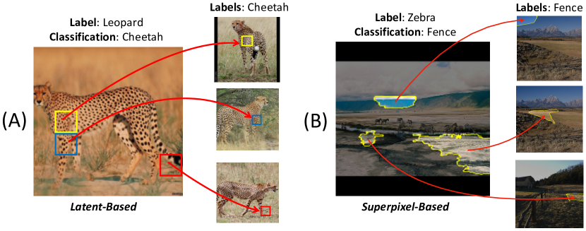
Figure 1: The Algorithms: (A) Our latent-based algorithm explains a misclassification of “Leopard” as “Cheetah” from the ImageNet dataset using three feature “parts” of the image, and linking them to where they were learned from in the training data. The explanation can be parsed as “I think the image is a Cheetah mainly because of these three features which remind me of Cheetahs that I have seen before”, thus communicating the classifier got confused because of similar spots and body parts on the two animals. (B) The superpixel-based algorithm explains a misclassification of “Zebra” as “Fence” on ImageNet in a similar way, where the explanation shows the AI learned a bias correlating “blue background” and “grassy fields” with “Fence”, causing the misclassification, thus communicating the AI has learned bad spurious features to identify the class “Fence”.

2 Related Work

There are three points we make prior to our literature review which benefit from clarification. Firstly, XAI can be roughly divided into pre-hoc interpretability and post-hoc explanations Rudin et al. (2022), CBR has been used for the former Kenny and Keane (2021), and for the latter Papernot and McDaniel (2018). Prior work in pre-hoc interpretability has isolated multiple clear feature “parts” in an image by learning prototypical features Chen et al. (2019), but these techniques often lose accuracy and are highly model specific; we are inspired by these works, but are interested here in developing similar algorithms for post-hoc explanation, so that they may be used to explain to any ANN, and never lose model accuracy. Secondly, the two prevalent theories in psychology for how humans categorize objects are exemplar and prototype theory Werner and Rehkämper (2001), this is mimicked in the AI literature where CBR either uses the entire training data for explanations Kenny and Keane (2019), or distils it into prototypical examples Kim et al. (2014), this paper is only related to the prior literature, and not be be entangled with the latter. Thirdly, although our work bears certain resemblance to work in the counterfactual literature Goyal et al. (2019), here we are concerned with similarity-based explanation Hanawa et al. (2021), not contrastive.

2.1 CBR and Feature Highlighting

Work combining feature-highlighting with CBR can be traced back to Patro & Namboodiri Patro and Namboodiri (2018), but it was constrained to a specific architecture, and the task of question & answering, and thus it is not a generalizable solution to the problem we are concerned with. In other work, Kenny & Keane Kenny and Keane (2019) proposed Feature Activation Maps (FAMs), to show similar heatmaps in a test image and nearest neighbor for CBR-based explanation. However, FAMs are constrained to specific ANN architectures and can not independently isolate multiple different features. Moreover, FAMs were not comparatively evaluated either computationally (which we rectify in Section 4), or in user studies, making it difficult to gauge the utility of FAMs. Most recently, Crabbé et al. Crabbé et al. (2021) proposed an ANN agnostic method, but it does not highlight regions in a test instance, and it computationally struggles beyond relatively simply domains such as MNIST where explanations are not heavily desired, casting its wider applicability into question. Considering this, there is a large gap in the literature for a general, well performing, post-hoc CBR method to attribute multiple feature “parts” of an image to corresponding parts of the explanatory cases found. Moreover, the technique(s) should be thoroughly evaluated in rigorous computational trials to verify the explanation fidelity, which we conduct in Sections 4 and 5.

2.2 User Evaluation

There is sparse work on user evaluation combining CBR and feature highlighting. Rymarczyk et al. Rymarczyk et al. (2021) continued the work of ProtoPNet Chen et al. (2019) and showed their highlighted features were more distinctive to users. However, these authors didn’t evaluate the effect of an explanation, but instead whether users found the features distinctive for a class, and crucial details (e.g., number of users) were omitted. Crabbé et al. Crabbé et al. (2021) conducted a user study, but it was really just a pilot (N=10), and there was no significance testing or control. In light of this, there is a requirement for a well conducted, thorough user trial to test the effectiveness of combining CBR and feature highlighting. Such a study should assess the effect such explanations have on end-users to ultimately verify their usefulness to people, which we orchestrate in Section 6.

2.3 Contributions

This paper’s main contribution is the proposal of two algorithms in Section 3 which can allow the attribution of multiple independent feature “parts” of a test image to other parts of the explanatory nearest neighbors found in post-hoc CBR exemplar-based explanation (see Figure 1 for examples of these two algorithms). As an aside, the evaluation of our algorithms also represents the largest-ever ablation tests comparing popular saliency-based XAI methods in the literature, which used the ILSVRC dataset encompassing 1 Million+ images. Most importantly however, Section 6 contributes the first user study purposefully designed to evaluate such explanation strategies in a concrete setting.

3 Method

In this section we introduce our two algorithms for isolating multiple clear feature “parts” in a test image, and linking them directly to where they were learned from in the training data. The first algorithm is an agnostic method for Convolutional Neural Networks (CNNs), and the second is a fully generalizable, agnostic method for all ANNs which uses superpixels. First however, in preparation, we detail our definitions and assumptions used in the subsequent formalization.

3.1 Definitions & Assumptions

Let a test image be denoted as $I$, and the ANN we wish to explain as $f(.)$. Assuming a neural net instantiation of this function with a final linear layer, we may decompose $f$ into an encoder $f_{enc}$, alongside the last layer with weights $\bm{W}$ and bias $\bm{b}$ as follows: $f(I)=\bm{W}f_{\text{enc}}(s)+\bm{b}$. Notably, this encoder $f_{enc}$ outputs a latent vector of the input image $I$, which we denote as $x$, this represents a high level representation of the image. Hence, we can denote the function as:

$$\begin{gathered}f(I)=xW+b.\end{gathered}$$ (1)

In the case of CNN architectures, $f_{enc}$ can be further broken down into convolutional layers $g(.)$, and the final transformation operation $t(.)$ which outputs $x$. The output of $g(.)$ is always a matrix $C\in{\rm I\!R}^{(h,w,d)}$, and the precise operation of $t$ is not important to our formalization, any generic transformation (e.g., a pooling layer or linear transformation) will work. Thus, in the case of CNNs the function can be written as:

$$\begin{gathered}f(I)=t(g(I))W+b\quad\text{where}\quad t(g(I))=x.\end{gathered}$$ (2)

Lastly, we assume the presence of some function $k(.)$ to retrieve a pool of $n$ nearest neighbors of a query $x$ from the training data $D$, all of which are scanned to find where the important feature “parts” in the query were learned from which caused the classification. In theory, the larger $n$ is, the better the explanation will be, as we can have more options to find the best match for the feature(s) in the query image, but due to computational constraints we limited it to $n=50$.

Algorithm 1 Latent-Based

1:$f(.);$ CNN to-be-explained

2:$I;$ Test Image

3:$D;$ Training Dataset

4:$m(.);$ Activation map algorithm (e.g., FAM)

5:Get Convolutional Output, $C\in{\rm I\!R}^{(h,w,d)}\leftarrow g(I)$

6:Get Activation Map; $M\in{\rm I\!R}^{(h,w)}\leftarrow m(f,I)$

7:Get Pool of $n$ Nearest Neighbors; $\{x_{i}\}_{i=1}^{n}\leftarrow k(f_{enc}(I),D)$

8:Select the segment $C_{i,j}\in{\rm I\!R}^{(1,1,d)}$ with the maximum saliency $M_{i,j}$ as $\omega_{test}$.

9:for $x_{i}\in\{x_{i}\}_{i=1}^{n}$ do

10:     $C_{x}\in{\rm I\!R}^{(h,w,d)}\leftarrow g(x_{i})$

11:     for $i$ in range $h$ do

12:         for $j$ in range $w$ do

13:              $\omega_{c}\leftarrow C_{i,j}\in{\rm I\!R}^{(1,1,d)}$

14:              Record $L_{2}$ distance $l=\|\omega_{c}-\omega_{test}\|^{2}_{2}$

15:         end for

16:     end for

17:end for

18:Select the neighbor $n$ with segment $i,j$ which minimized Eq. (3).

3.2 Latent-Based Algorithm

The first algorithm takes inspiration from Chen et al. Chen et al. (2019), but in a post-hoc (rather than their pre-hoc) manner. For a given test image $I$, a final representation $C\in{\rm I\!R}^{(h,w,d)}$ is extracted after all convolutional layers, where $h$ and $w$ represent the height and width of the output, respectively, and $d$ the number of kernels. This may be broken down into regions shaped $h_{1}\times w_{1}\times d$, where $h_{1}<h$ and $w_{1}<w$. These regions may be upsampled to the size of the test image to visualize them as a “box” [e.g., Fig. 4(A)], which is the region in pixel-space that corresponds to this region in $C$. To select salient areas in the test image, the presence of some activation map $M_{test}\in{\rm I\!R}^{(h,w)}$, giving the importance of each spatial region in $C$ is assumed (e.g., FAMs). Next, by selecting the most positive salient region(s), one can isolate the test image salient box region $\omega_{test}\in{\rm I\!R}^{(1,1,d)}$.

Algorithm 2 Superpixel-Based

1:$f(.);$ ANN to-be-explained

2:$I;$ Test Image

3:$D;$ Training Dataset

4:$S(.);$ Superpixel Algorithm

5:Get Test Image Superpixels $\{p_{i}\}_{i=1}^{n}\leftarrow S(I)$

6:Upsample $\{p_{i}\}_{i=1}^{n}$

7:$\{l_{i}\}_{i=1}^{n}\leftarrow\{f_{enc}(p_{i})\}_{i=1}^{n}$

8:Get Pool of $n$ Nearest Neighbors; $\{x_{i}\}_{i=1}^{n}\leftarrow k(f_{enc}(I),D)$

9:for $n_{i}\in\{x_{i}\}_{i=1}^{n}$ do

10:     $S_{n}\leftarrow S(x)$

11:     for $s_{i}\in S_{n}$ do

12:         Occlude $n_{i}!=s_{i}$

13:         $\hat{y}=f(n_{i})$

14:         $\hat{y}=argmax(f_{enc}(I)W+b)$

15:         $m_{i}=argmax(f_{enc}(s_{i})W+b)$

16:         Upsample $s_{i}$

17:         $l_{i}=f_{enc}(s_{i})$

18:     end for

19:end for

20:Select neighbor $n$ with segment $l_{i}$ which minimizes Eq. (4).

Now the task is to find a similar region in the training data $\omega_{nn}$ where the salient feature was “learned” from. In the pool of $n$ nearest neighbors, let $C_{(n,i,j)}$ represent some region $\omega\in{\rm I\!R}^{(1,1,d)}$ in the final convolutional layer, with the neighbor indexed by $n$, and its spatial position in $C_{n}$ indexed by $i$ and $j$. These $n$ images have their $C$ representation searched to find the closest match to $\omega_{test}$ using the $L_{2}$ norm to find $\omega_{nn}$. Crucially, the feature is constrained to its relative importance. Specifically, considering each NN’s $M_{n}$, only those regions which satisfy the constraint of being higher than $max(M_{n})\times\alpha^{-1}$ are considered to find $\omega_{nn}$ by minimizing:

$$\begin{gathered}\underset{n,i,j}{\arg\min}\quad\|\omega_{test}-C_{(n,i,j)}\|_{2}\quad\\ \textrm{s.t.}\quad M_{(n,i,j)}>max(M_{n})\times\alpha^{-1}.\end{gathered}$$ (3)

Alpha ensures $\omega_{nn}$ is critical to the classification, but as it is a hyperparameter we computationally explore its optimal value in Section 5.

3.3 Superpixel-Based Method

This second algorithm uses superpixels to realize a more ANN-agnostic method. The only assumption is that the ANN extracts a latent representation $\vec{x}\in{\rm I\!R}^{(d)}$ in its penultimate layer before a linear output layer. This is important because other similar methods are not ANN agnostic Kenny and Keane (2019); Chen et al. (2019), and would fail to explain state-of-the-art Vision Transformers  Dosovitskiy et al. (2020). Specifically, LIME Ribeiro et al. (2016) is used to find salient regions of a test image, and it’s neighbors are scanned to find the closest match. However, at scale, LIME was too slow to work on the pool of neighbors, so we developed a new method which we now detail.

Formally, consider a test image’s most salient superpixel region $\omega_{test}\in{\rm I\!R}^{(d)}$, where $d$ is the number of extracted features in the penultimate layer. To acquire each regions latent representation, (1) all other regions were occluded, (2) the region is upsampled to the ANN’s input size whilst keeping the aspect ratio, and (3) it is passed through the network to record it’s representation in layer $x$. To find a matching region in the training data $\omega_{nn}$ where this feature was “learned”, let $S_{(n,i)}$ be the representation $\omega\in{\rm I\!R}^{(d)}$ of a superpixel segment $i$ in the NN $n$. Moreover, let $M_{(n,i)}$ be each region’s saliency, which is acquired by (1) occluding the rest of the image, (2) passing it through the network, and (3) recording the logit value in the originally predicted class by the network. The $n$ images have their $S$ representations searched to find the closest match to $\omega_{test}$ using the $L_{2}$ norm to find $\omega_{nn}$. Importantly, this region is constrained to its relative importance, only regions with saliency higher than $max(M_{n})\times\beta^{-1}$ are considered to find $\omega_{nn}$ by minimizing:

$$\begin{gathered}\underset{n,i}{\arg\min}\quad\|\omega_{test}-S_{(n,i)}\|_{2}\quad\\ \textrm{s.t.}\quad M_{(n,i)}>max(M_{n})\times\beta^{-1}.\end{gathered}$$ (4)

The beta constraint ensures $\omega_{nn}$ is critical to the classification. However, again as this is a hyperparameter, its value must be justified though rigorous computational evaluation which we do in Section 5.

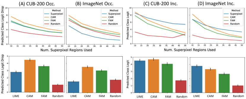
Figure 2: Expt. 1 Results: Salient Feature Occlusion (Occ.) and Inclusion (Inc.): The first row of lineplots show a comparison of the four different methods proposed in Section 3. The second row shows a comparison of the three latent-based methods against LIME, to see the difference between LIME and our superpixel method. Overall, all methods do significantly better than random occlusion/inclusion, LIME performs similarly to our superpixel method, and CAM performs best. Standard Error bars are shown.

4 Experiment 1: Test Image Highlighting

Kenny & Keane Kenny and Keane (2019) proposed FAMs as (to the best of our knowledge) the only post-hoc method thus far for CBR-based XAI linking an area in the test image to an area in the training one, but the method has two clear drawbacks. Firstly, FAMs cannot isolate multiple clear feature “parts” for an explanation, despite this being argued as a better approach Chen et al. (2019). Secondly (and most importantly), FAMs were assumed to be the best method for adding feature highlighting to CBR post-hoc, as no comparative tests were ever performed by the authors, despite recent criticisms of feature attribution methods Adebayo et al. (2018); Zhou et al. (2022). We address the first issue in our algorithms proposed in Section 3 (which allow multiple clear feature parts to be used in an explanation), and the second issue is addressed by comparing FAMs against Class Activation Mapping (CAM), Random maps, LIME Ribeiro et al. (2016), and our own superpixel method in Section 3.3 in large a large-scale ablation study next.

4.1 Method and Datasets

These tests worked via two methods, by (1) keeping the salient region in the pixel image (whilst occluding the rest), and (2) by occluding the salient region (and keeping the rest). In the first case, the method that produces the highest logit in the original predicted class does best after a forward pass in the ANN, and in the second the method which produces the highest drop is best (n.b., if the prediction changes the same logit is recorded). For a fair test, the second ablation method was included because the first may be biased towards our Superpixel method which isolate salient regions based on maximizing such logit values [though results show this is not the case, see Fig. 2(D)]. To find equally sized regions between methods, a superpixel segment is first isolated, then the latent-based heatmaps are found by up-sampling their activation maps to the pixel-space, and isolating an equally sized region to the superpixel taken from the parts of highest saliency. Two datasets CUB-200 Welinder et al. (2010) and ImageNet Deng et al. (2009) were used, with the former fine-tuning ResNet34, and the latter using a pre-trained ResNet50 (see Appendix). The experiment is repeated with different segmentation options for superpixels (which changed how big the superpixel regions – feature parts – are). Tests used the first 500 validation images.

4.2 Results

Fig. 2(A/B) shows the results of occluding (Occ.) the region, and Fig. 2(C/D) of including (Inc.) it (and occluding the rest of the image). The top row shows the results of comparing the four saliency methods discussed in Section 3, whilst the bottom shows comparisons of latent-based methods against LIME. Note these LIME comparisons correspond to $\approx$5% of the test image being isolated, which corresponds to $\approx$30 superpixels used in the top row tests. Overall, all methods are significantly better than random. Superpixels perform best for inclusion, especially when the segment number is $>$ 30, but CAMs/FAMs are more consistently good (although FAMs are worse than CAMs). Perhaps most notably, all methods perform poorly when occluding in ImageNet, likely because ImageNet has many objects in an image which are used for classification, and removing a small region has little effect. All superpixel methods in particular do bad here (i.e., worse than random), likely because they still maintain the “shape” of the object during occlusion, whilst the latent-based methods (including random) always occlude smoother shapes which distorts the objects more. This hypothesis is likely true because this was not repeated in the inclusion experiments, and consistent across all superpixel methods, which is notable because LIME is thought to deliver good explanations Jeyakumar et al. (2020). So, taking the results as a whole, it is safe to posit that whilst all methods work well in isolating important regions in a test image, CAM does best overall.

5 Experiment 2: Linking to Training Data

The purpose of this experiment is to isolate the best hyperparameter values for $\alpha$ and $\beta$ in equations 3 and 4, respectively. Knowing these optimal values ensures that the highlighted regions in the explanatory cases are actually relevant to the classification, and not actively misleading end-users. Hence, potential explanatory features in the nearest neighbors “used” in classification were occluded in the training data, then the networks were fine-tuned, which allows us to see what regions are necessary to maintain test performance. First, $\alpha$ and $\beta$ are varied from one to infinity [the latter considered as all positive salient regions in Eq. (3/4)] to see their optimal value, then a comparative test is done. Eq. (3) and (4) cannot be directly compared because alpha and beta are relative constraints. However, a comparison was accomplished by (1) varying alpha, (2) closely matching the occlusion area by gradually introducing superpixels (in order of highest saliency value), and (3) readjusting the size of the latent-based methods area to match the superpixel area. In essence, we are doing a grid search to find the optimal values for the $\alpha$ and $\beta$ hyperparameters discussed in Section 3, to optimally instantiate our algorithms.

For each hyperparamter value, the networks were fine-tuned for 2500 iterations and test-accuracy sampled every 50, as this was found sufficient for our purposes (20 epochs were tested with no notable differences). This procedure gives us an indication of which regions of the training data images are actually responsible for test predictions (and what $\alpha$ and $\beta$ are best). As a sanity check, the networks were also tested by completely occluding all training images and were reduced to random guessing after 2500 iterations, thus verifying that features are being “unlearned”. Note this experiment requires a constant value for superpixel segmentation, so 30 was chosen as it was the smallest value which generalized best in Expt. 1.

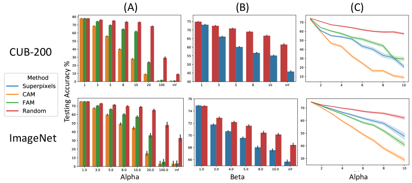
Figure 3: Expt. 2 Results: (A) Exploring the hyperparameter choice for alpha, (B) doing similar tests for beta. (C) A direct comparison between methods by varying alpha. Results show that all methods are better than the random baseline in nearly every test, FAMs and Superpixels are interchangeable, and CAM seems the best method.

5.1 Results

Fig. 3(A) shows $\alpha$ varied, where values between 3-20 produce statistically better results for CAM against FAM/Random (2-tailed ind. t-test; $p$ $<$ 0.05). Fig. 3(B) shows what happens to superpixels v. random when varying $\beta$, where an infinite value (i.e., using all positive superpixels) produces the most divergent results for CUB-200 (Acc. Rand=61.55 v. Superpixel=45.86) and ImageNet (Acc. Rand=68.41 v. Superpixel=65.68). Note even with $\beta=inf$ only $\sim$66% of the images are occluded in ImageNet on average for our superpixel method, which roughly equates to CAM at $\alpha=5$, so there is not a huge disparity when considering this. Fig. 3(C) shows a direct comparison, where CAM performs best, with FAMs and superpixels being interchangeable, and all methods outperforming the random baseline. Finally, it should be noted these are empirical tests on retrained networks and are to be treated with some caution, but similar tests have been done and accepted Hooker et al. (2019). Overall, these results show a converging results that CAM again is the most discriminative.

Computational Conclusions.

Expts. 1-2 showed CAM-based explanations to be best for locating discriminative regions, but superpixels can generalize beyond CNNs Du et al. (2022), and still performed well (but we evaluated them on CNNs so comparative tests were possible). Importantly, FAMs Kenny and Keane (2019) were shown to be less discriminative than CAM, and cannot generalize like Superpixels, thus our tests show a clear improvement upon previously proposed approaches. For hyperparameters, latent-based CAM should use $\alpha$=5, as it worked well and has other support Zhou et al. (2016). For superpixel methods, LIME should be used to find test image “parts” (it does slightly better than our superpixel method in Expt. 1), but our superpixel method should be used for finding the matching regions in the training data pool since it performs similarly, is much faster, and has experimental evidence in Expt. 2. Superpixel segmentation of 30 and $\beta$=$\infty$ in superpixels is recommended as it generalizes best. Lastly, note the latent-based algorithm is faster to compute compared to the superpixel one ($\sim$2sec v. $\sim$60; $n$=10; CPU).

6 User Study

Although highlighting CBR explanations with important features has become increasingly popular Chen et al. (2019); Kenny and Keane (2019); Crabbé et al. (2021); Kenny and Keane (2021); Donnelly et al. (2021), there exists no substantial user study which demonstrates whether such explanations have a useful effect on people. So, rather than focusing on comparative testing between various methods, this study examines the more pressing and fundamental question of whether such explanations have a different effect on people than traditional case-based explanation. Hence, a user study (N=163) was run to test case-plus-saliency v. case-only explanations, using CAM with $\alpha=5$, a neighbor pool of size $n$=50, and a single highlighted feature. Previous similar user studies have shown that case-based explanations changed people’s perceptions of the correctness of misclassifications Kenny et al. (2021). Hence, here it is examined whether explanatory examples with or without saliency (i.e., a Box v NoBox manipulation; see Fig. 4) do the same. So, the study presented participants with 32 test-images from the ImageNet dataset (i.e., 24 misclassifications, with 8 “fillers” that were correct classifications for attention checks) and were asked to make classification-correctness judgements of these items presented alongside one of the two explanation-types (NoBox or Box; i.e., no saliency or saliency). The 24 misclassifications were randomly divided into two material sets (A-set and B-set) to counterbalance the experiment; so, one group (N=82) received the A-set with case-only explanations (NoBox) and the B-set with case-plus-saliency explanations (Box) and the other group (N=81) received the A-set with case-plus-saliency explanations (Box) and the B-set with case-only explanations (NoBox; see Fig. 4(A) for example). The statistical analysis then collapsed across these counterbalanced groups controlling for the effects of the material-set.

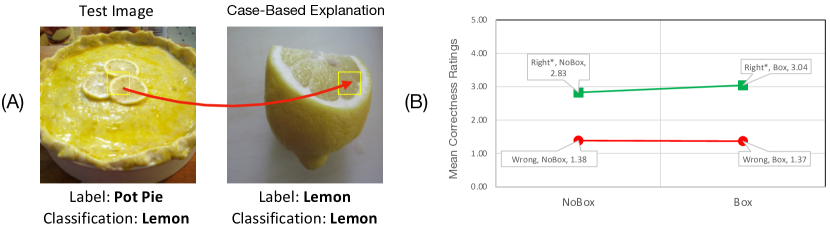
Figure 4: (A) A “Pot Pie” misclassified as “Lemon”. The explanation shows the test image and its relevant salient area alongside its explanatory nearest neighbor in the case-based explanation pointing to where it was “learned”. Glossed, the explanation says “I think this is a lemon, because it has a similar part to an image I saw before which I learned should be a lemon”. (B) Correctness ratings for material-set B broken out by “Right*” and Wrong classifications for the two explanation-types, NoBox (example-only) and Box (example-plus-saliency). Here, the Right*-Box ratings (M=3.04) are reliably different to the Right*-NoBox ratings (NoBox, M=2.83), reflecting people’s performance on ambiguous items in that material-set.

6.1 Method

Participants.

Participants (N=163) were recruited on Prolific.co. All were aged over 18, native English speakers, and lived in the U.S.A., U.K., or Ireland. Participants were paid £7.50/hr, which totalled £319.8. This N was chosen based on a power analysis for a low effect-size; this size was chosen because it was anticipated the addition of saliency “boxes” would have a quite nuanced effect over just explanation-by-example due to it already being heavily preferred by users Jeyakumar et al. (2020). This study passed ethics review of the institution ref. LS-E-19-148-KennyKeane.

Materials.

Twenty-four misclassifications were randomly sampled. These were actual test-image errors when the classification differed from the ground truth. The twin-system method Kenny and Keane (2019) was applied to find a nearest-neighbor CBR-explanation, and our latent-based algorithm (i.e., Section 3.2) was used to identify highlighted regions [shown as a Box; see Fig. 4(A)]. The materials were randomly assigned to two different sets (A-set and B-set) and counterbalanced. Importantly, the sampling constrained the images to be both varied and those involving classes people could easily understand (e.g., snail, lemon, etc.).

Procedure.

After being told the system “learned” to classify objects in images, people were told they would be shown several examples of its classifications (see Appendix). Their task was to rate the correctness (i.e., the question was “The program’s labelling of the image is correct.”) of the classification on a 5-point Likert-scale from “I disagree strongly” (1) to “I agree strongly” (5). Each participant was shown 24 misclassifications (12 NoBox and 12 Box explanations) along with 8 filler items that were all correct classifications appearing every fourth question for attention checks. The 24 incorrect items were randomly re-ordered for each person.

6.2 Results & Discussion

No users failed the attention checks. The analysis showed the items in the B-set that received the example-plus-saliency explanation (Box; M=1.93) were rated as less-incorrect than their equivalent items in Set-A (M=1.77); this difference between B-set-Box and A-set-Box was statistically reliable, $t$(161) = 2.15, $p$ = 0.03, 2-tailed using a two-sample t-test. This result shows that image-explanations with feature highlighting impact people’s perception of correctness for misclassifications, but only for certain items.

An ad-hoc analysis of this effect discovered that in both material-sets there were ambiguous materials that people consistently rated as more correct (i.e., mean $>$ 2) even though the ground-truth identified these items as incorrect (3/12 in A-set and 4/12 in B-set). So, the items were partitioned into two new categories, namely “Right*”-items (that people rated as more “correct”, even though they were incorrect classifications) and Wrong-items (that people confidently rated as incorrect, when they were incorrect) and then re-analyzed for each material-set (n.b., the asterisk on “Right*” signifies they are not really “Right”). This partitioning was objectively verified by clustering the material means (using $k$-means) 500 times and finding that the data consistently forms these two groups. Fig. 4(B) shows that in the B-set the correctness rating for the Right*-misclassifications with example-plus-saliency explanation (Box, M=3.04) is reliably higher than that for the example-only explanation (NoBox, M=2.83), $t$(162) = 1.8, $p$ = 0.036, using 1-tailed, two-sample t-test. This may raise ethical concerns as feature highlighting could give users the impression that “incorrect” classification’s seem less incorrect, but this concern is likely due to the fact that some images could plausibly be labelled as multiple different classes. To elaborate, Fig. 4(A) shows an example of these Right* items where a picture of a “Pot Pie” (decorated with lemons) is misclassified as “Lemon”. Here, the saliency explanation shows an image of a lemon and the “pulp of the lemon” as the feature that influenced the classification. When people see this explanation, it shows what the CNN is focusing on (i.e., the “Lemon” instead of the “Pot Pie”), leading them to rate the CNN classification as more correct (which makes sense), an effect which does not occur without using feature “parts” in the explanation.

7 Conclusion

This work advances two novel case-based approaches to (i) highlight important regions in a test image and (ii) link these regions back to corresponding relevant regions in the training data. Unlike previous work, our approach is not constrained to specific architectures and can highlight multiple regions in an ANN agnostic fashion. Large scale ablation testing revels that the proposed approaches are more faithful to the model and select more relevant regions in the training data than previous solutions. Results from a large scale user study indicate the utility of highlighting feature parts instead of just providing a relevant training example. Specifically, the study showed that the explanations help to appropriately calibrate people’s understanding of how correct a classifier is on ambiguous test images.

References

- Adebayo et al. [2018] Julius Adebayo, Justin Gilmer, Michael Muelly, Ian Goodfellow, Moritz Hardt, and Been Kim. Sanity checks for saliency maps. In Proceedings of the 32nd International Conference on Neural Information Processing Systems, pages 9525–9536, 2018.
- Chen et al. [2019] Chaofan Chen, Oscar Li, Daniel Tao, Alina Barnett, Cynthia Rudin, and Jonathan K Su. This looks like that: Deep learning for interpretable image recognition. Advances in Neural Information Processing Systems, 32:8930–8941, 2019.
- Crabbé et al. [2021] Jonathan Crabbé, Zhaozhi Qian, Fergus Imrie, and Mihaela van der Schaar. Explaining latent representations with a corpus of examples. Advances in Neural Information Processing Systems, 34, 2021.
- Deng et al. [2009] Jia Deng, Wei Dong, Richard Socher, Li-Jia Li, Kai Li, and Li Fei-Fei. Imagenet: A large-scale hierarchical image database. In 2009 IEEE Conference on Computer Vision and Pattern Recognition, pages 248–255, 2009.
- Donnelly et al. [2021] Jon Donnelly, Alina Jade Barnett, and Chaofan Chen. Deformable protopnet: An interpretable image classifier using deformable prototypes. arXiv preprint arXiv:2111.15000, 2021.
- Dosovitskiy et al. [2020] Alexey Dosovitskiy, Lucas Beyer, Alexander Kolesnikov, Dirk Weissenborn, Xiaohua Zhai, Thomas Unterthiner, Mostafa Dehghani, Matthias Minderer, Georg Heigold, Sylvain Gelly, et al. An image is worth 16x16 words: Transformers for image recognition at scale. arXiv preprint arXiv:2010.11929, 2020.
- Du et al. [2022] Xin Du, Benedicte Legastelois, Bhargavi Ganesh, Ajitha Rajan, Hana Chockler, Vaishak Belle, Stuart Anderson, and Subramanian Ramamoorthy. Vision checklist: Towards testable error analysis of image models to help system designers interrogate model capabilities. arXiv preprint arXiv:2201.11674, 2022.
- Goyal et al. [2019] Yash Goyal, Ziyan Wu, Jan Ernst, Dhruv Batra, Devi Parikh, and Stefan Lee. Counterfactual visual explanations. In International Conference on Machine Learning, pages 2376–2384. PMLR, 2019.
- Hanawa et al. [2021] Kazuaki Hanawa, Sho Yokoi, Satoshi Hara, and Kentaro Inui. Evaluation of similarity-based explanations. In Proceedings of the Ninth International Conference on Learning Representations, 2021.
- Hooker et al. [2019] Sara Hooker, Dumitru Erhan, Pieter-Jan Kindermans, and Been Kim. A benchmark for interpretability methods in deep neural networks. Advances in Neural Information Processing Systems, 32:9737–9748, 2019.
- Jeyakumar et al. [2020] Jeya Vikranth Jeyakumar, Joseph Noor, Yu-Hsi Cheng, Luis Garcia, and Mani Srivastava. How can i explain this to you? an empirical study of deep neural network explanation methods. Advances in Neural Information Processing Systems, 33, 2020.
- Kenny and Keane [2019] Eoin M Kenny and Mark T Keane. Twin-systems to explain artificial neural networks using case-based reasoning: Comparative tests of feature-weighting methods in ann-cbr twins for xai. In Twenty-Eighth International Joint Conferences on Artifical Intelligence (IJCAI), Macao, 10-16 August 2019, pages 2708–2715, 2019.
- Kenny and Keane [2021] Eoin M Kenny and Mark T Keane. Explaining deep learning using examples: Optimal feature weighting methods for twin systems using post-hoc, explanation-by-example in xai. Knowledge-Based Systems, page 107530, 2021.
- Kenny et al. [2021] Eoin M Kenny, Courtney Ford, Molly Quinn, and Mark T Keane. Explaining black-box classifiers using post-hoc explanations-by-example: The effect of explanations and error-rates in xai user studies. Artificial Intelligence, page 103459, 2021.
- Kim et al. [2014] Been Kim, Cynthia Rudin, and Julie A Shah. The bayesian case model: A generative approach for case-based reasoning and prototype classification. In Advances in neural information processing systems, pages 1952–1960, 2014.
- Leake and McSherry [2005] David Leake and David McSherry. Introduction to the special issue on explanation in case-based reasoning. The Artificial Intelligence Review, 24(2):103, 2005.
- Papernot and McDaniel [2018] Nicolas Papernot and Patrick McDaniel. Deep k-nearest neighbors: Towards confident, interpretable and robust deep learning. arXiv preprint arXiv:1803.04765, 2018.
- Patro and Namboodiri [2018] Badri Patro and Vinay P Namboodiri. Differential attention for visual question answering. In Proceedings of the IEEE conference on computer vision and pattern recognition, pages 7680–7688, 2018.
- Ribeiro et al. [2016] Marco Tulio Ribeiro, Sameer Singh, and Carlos Guestrin. Why should i trust you?: Explaining the predictions of any classifier. In Proceedings of the 22nd ACM SIGKDD international conference on knowledge discovery and data mining, pages 1135–1144. ACM, 2016.
- Rudin et al. [2022] Cynthia Rudin, Chaofan Chen, Zhi Chen, Haiyang Huang, Lesia Semenova, and Chudi Zhong. Interpretable machine learning: Fundamental principles and 10 grand challenges. Statistics Surveys, 16:1–85, 2022.
- Rymarczyk et al. [2021] Dawid Rymarczyk, Łukasz Struski, Michał Górszczak, Koryna Lewandowska, Jacek Tabor, and Bartosz Zieliński. Interpretable image classification with differentiable prototypes assignment. arXiv e-prints, pages arXiv–2112, 2021.
- Welinder et al. [2010] Peter Welinder, Steve Branson, Takeshi Mita, Catherine Wah, Florian Schroff, Serge Belongie, and Pietro Perona. Caltech-ucsd birds 200. In Computation & Neural Systems Technical Report. 2010-001. California Institute of Technology, Pasadena, CA., 2010.
- Werner and Rehkämper [2001] Christian W Werner and Gerd Rehkämper. Categorization of multidimensional geometrical figures by chickens (gallus gallus f. domestica): fit of basic assumptions from exemplar, feature and prototype theory. Animal Cognition, 4(1):37–48, 2001.
- Zhou et al. [2016] Bolei Zhou, Aditya Khosla, Agata Lapedriza, Aude Oliva, and Antonio Torralba. Learning deep features for discriminative localization. In Proceedings of the IEEE conference on computer vision and pattern recognition, pages 2921–2929, 2016.
- Zhou et al. [2022] Yilun Zhou, Serena Booth, Marco Tulio Ribeiro, and Julie Shah. Do feature attribution methods correctly attribute features? In Proceedings of the AAAI Conference on Artificial Intelligence, volume 36, pages 9623–9633, 2022.