On optimal control of reflected diffusions

Abstract.

We study a simple singular control problem for a Brownian motion with constant drift and variance reflected at the origin. Exerting control pushes the process towards the origin and generates a concave increasing state-dependent yield which is discounted at a fixed rate. The most interesting feature of the problem is that its solution can be more complicated than anticipated. Indeed, for some parameter values, the optimal policy involves two reflecting barriers and one repelling boundary, the action region being the union of two disjoint intervals. We also show that the apparent anomaly can be understood as involving a switch between two strategies with different risk profiles: The risk-neutral decision maker initially gambles on the more risky strategy, but lowers risk if this strategy underperforms.

1. Introduction

This paper explores an unanticipated and, as of yet, unknown feature of a class of optimal control problems for reflected diffusions. Our focus centers on the process $X=\{X_{t}\}_{t\geq 0}$ defined as

$$X_{t}=x+\mu t+\sigma W_{t}-{{\xi}}_{t}+{\mathscr{L}}_{t},\quad t\geq 0,$$ (1)

where $x\geq 0$ is an arbitrary initial condition, $\mu$ and $\sigma$ are constants, $W$ is a standard Brownian motion, and where ${{\xi}}$, the control process, is right-continuous, non-decreasing and non-anticipative (i.e., independent of future increments of $W$). Given $W$ and ${{\xi}}$, the non-decreasing process ${\mathscr{L}}$ is constructed so as to enforce a lower reflecting barrier at $0$. For the existence and characteristics of such a process, see [6, § 1] or [13, § 3].

Our problem can be interpreted in different ways (discussed below), but we are especially interested in the case when $X$ models the water level in a dam having a reflecting lower boundary (cf. [3, 34, 35]). In the absence of control, the water level evolves according to reflected Brownian motion with constant drift and variance. Extracting an amount $\varepsilon$ of water causes the water level to drop by the same amount and generates a yield of $\eta(X)\varepsilon$. Assume, as in [35], that the extraction costs increase with depth in such a way that $\eta(x)=(1-\frac{1}{x})^{+}$. Thus, $\eta$ vanishes in a neighborhood of zero and is concave increasing on its support. The problem (stated formally in Section 2) is to maximize the expected total yield over an infinite time horizon for an exogenously given discount rate of $r>0$.

As we show in this paper, despite the problem’s simplicity, its solution can be quite complicated. One might anticipate that control should be exerted when the state process exceeds a certain threshold $b>0$. Such a control policy serves to enforce an upper reflecting barrier at $b$. For most values of the three parameters ($\mu,\sigma$, $r$), the optimal policy indeed takes this simple form. Yet for a non-empty subset of the parameter space, the optimal policy is a ‘band policy’ with three boundaries, $b<\theta<\lambda$. A barrier is enforced at $\lambda$ until $X$ drops to $\theta$, and a barrier is enforced at $b$ from that point onward (see Figure 1).

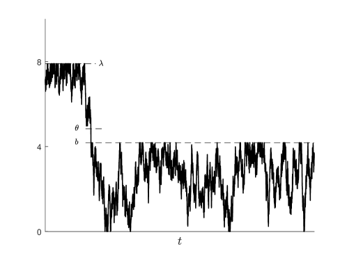
Figure 1. A sample path of (1) under optimal control.

This result, which is conjectured by Liu et al [24], appears eccentric enough to call the model into question. (Incidentally, of the people that were presented with the problem in discussion, none anticipated the stated result, and, when informed of the result, not one was able to provide a rationale or empiric basis for operating with three thresholds.) Liu et al [24] suggest that the result is caused by the choice of marginal yield function. A proper explanation of the result must in some way account for the reflection, however, because we will see that it is always optimal to use a single barrier in the absence of reflection, for any concave yield function (see Remark 6). With the benefit of hindsight and the recent results of Ferrari [14], we can interpret the band policy portrayed in Figure 1 as involving a switch between two modes of operation with different risk profiles. We postpone its discussion to our concluding remarks (Section 6).

The problem studied in this paper is closely related to the problem of Karatzas and Shreve [23] in which a reflected Brownian motion is controlled by a process of bounded variation. Versions of this problem arise as inventory and asset management problems where the last two terms in (1) are interpreted as ‘withdrawals’ and ‘deposits’, respectively [33, 12, 25, 15, 37]. The form of the optimal policy in these problems is well understood in the case when the marginal yield function is constant. In this case, the optimal policy (when one exists) involves a single upper barrier [32]. Ferrari [14] shows that the same holds true under a structural assumption on the yield function (see (7) below). The main contribution of this paper is to show that the optimal policy can be more complicated than anticipated.

We believe that our results will be of interest from a methodological perspective as well as from the point of view of applications. The methodological interest lies in the fact that the application of smooth fit becomes complicated when the structural condition from [14] is relaxed. More precisely, we find a partial lack of smooth fit, as the value function fails to be of class $C^{2}$ at the ‘repelling’ $\theta$-boundary. Smooth fit has proven highly effective in solving optimal control problems and there is a growing literature on its limitations [28, 17, 16, 9, 10]. It is known, for instance, that smooth fit may fail due to the non-convexity of the cost structure [10] or the irregularity of the scale function of the underlying diffusion [28]. We present what to our knowledge is the first example demonstrating that a lack of smooth fit can arise as a consequence of exogenous reflection.

Our practical interest in understanding the phenomenon portrayed in Figure 1 is motivated by the popularity of the reflected Brownian model (1) in applications of the aforementioned types. In applications, one typically wants to determine a single threshold at which control should be exerted. (We mention an exception to this rule in Section 6.) Much research effort has in fact focused on identifying conditions on the yield structure that guarantee the existence of optimal policies of barrier type [29, 14, 35, 1, 20]. There thus seems to be disagreement between the management of real world systems on the one hand and the model’s prescriptions on the other. We believe that this may lead many to wonder (as we have) if the phenomenon portrayed in Figure 1 is signalling a flaw in the model of how such systems evolve in time. As indicated above, we will suggest, on the contrary, that the phenomenon provides insight. At the same time, our results indicate that the phenomenon is very rare and that there is little to be gained by operating with three thresholds (see Remark 5). In practice, the structural condition from [14] thus seems rather unrestrictive.

The paper is organized as follows: In the next section we give a precise statement of the problem and of our main result. Section 3 describes the methods that we will use and presents some auxiliary results. As in [24], we use a guess-and-verify approach relying on a martingale formulation of the dynamic programming principle. In Sections 4 and 5 we prove the main result. Finally, in Section 6 we discuss the mode switch alluded to above.

2. Problem formulation and statement of results

2.1. Problem formulation

To formulate our problem in precise terms, we take as primitive a Brownian motion $W=\{W_{t}\}_{t\geq 0}$ on a complete probability space with a filtration $\{\mathscr{F}_{t}\}$ satisfying the usual assumptions. The right-continuous, non-decreasing, $\{\mathscr{F}_{t}\}$-adapted processes form the class ${\mathscr{A}}$ of admissible control policies. Given ${{\xi}}\in{\mathscr{A}}$, the non-decreasing process ${\mathscr{L}}$ pushes by the minimal amount needed to ensure that (1) stays non-negative. In the absence of control, ${\mathscr{L}}$ is just the local time at $0$ of a Brownian motion starting at $x$. In general, ${\mathscr{L}}$ may jump if needed to prevent $X$ from jumping across the origin. However, we will primarily be interested in policies for which ${\mathscr{L}}$ is a.s. continuous as a function of $t$.

In view of previous studies of similar problems (see [5, 4, 22]), we are especially interested in policies with singular (local-time-like) parts. Such a policy is here characterized by a closed set $\mathcal{A}\subset(0,\infty)$ of action and its complement (the region of inaction) as follows: If $X$ starts in the interior of $\mathcal{A}$, then control is exerted to instantaneously get to the boundary of $\mathcal{A}$; if $X$ starts in the complement of $\mathcal{A}$, then control is exerted by the minimal amount needed to prevent $X$ from crossing the boundary of $\mathcal{A}$. If ${{\xi}}$ has action region $[b,\infty)$, then ${{\xi}}$ serves to enforce an upper reflecting barrier at $b$. We refer to such a policy as a barrier policy. The barrier policy with threshold $b$ is denoted by ${{\xi}}^{(b)}$.

If ${{\xi}}\in{\mathscr{A}}$ is a.s. continuous as a function of $t$, the total discounted yield that ${{\xi}}$ generates over the interval $[s,t)\subset[0,\infty)$ is given by the random variable

$$\int_{s}^{t}e^{-{r}u}\eta(X_{u})d{{\xi}}_{u}.$$ (2)

For possibly discontinuous ${{\xi}}\in{\mathscr{A}}$, we are led to consider

$$\int_{[s,t)}e^{-{r}u}\eta(X_{u})\circ d{{\xi}}_{u}:= \int_{s}^{t}e^{-{r}u}\eta(X_{u})d{{\xi}}^{c}_{u}+\sum_{s\leq u<t}e^{-{r}u}\int_{X_{s}}^{X_{s_{-}}}\eta(u)du,$$ (3)

where ${{\xi}}^{c}$ is the continuous part of ${{\xi}}$ and where the sum is taken over the discontinuity points of ${{\xi}}$. The definition (3) represents the standard way of dealing with the fact that the Stieltjes integral (2) does not properly account for lump rewards generated at discontinuity points of ${{\xi}}$ [8, 36, 20]. If $s=0$ and ${{\xi}}_{0}>0$, the sum in (3) carries a leading term of $\int^{x}_{x-{{\xi}}_{0}}\eta(u)du$.

The value of ${{\xi}}\in{\mathscr{A}}$ is defined

$$V_{{\xi}}(x)=\mathbb{E}_{x}\int_{[0,\infty)}e^{-{r}t}\eta(X_{t})\circ d{{\xi}}_{t},$$ (4)

where $\mathbb{E}_{x}$ denotes expectation conditioned on the fact that $X$ starts at $x$. The problem is to maximize $V_{{\xi}}(x)$ over ${{\xi}}\in{\mathscr{A}}$. The value function, $V(x)$, is defined

$$V(x)=\sup_{{{\xi}}\in{\mathscr{A}}}V_{{\xi}}(x).$$ (5)

Our main result concerns the marginal yield function

$$\eta(x):=(1-\frac{1}{x})^{+}$$ (6)

from [24, 35]. Throughout, we make the following assumptions on $\eta$.

Assumption 1.

h

• $\eta\colon[0,\infty)\to[0,1]$ is increasing and concave on its support,

• $\eta(x^{\ast})=0$ for some $x^{\ast}>0$.

It is easy to show that $V$ would be infinite if $\eta(0)$ were strictly positive. 1 (ii) removes incentive to exert control near $0$ and ensures that $V$ is finite. A more general condition is formulated as Assumption 2.9 in [14].

2.2. Prior results

Aside from [24], the two works most closely related to our study are the papers by Zeitouni [35] and Ferrari [14]. Zeitouni [35] formulates and partially solves the problem that we have stated. More precisely, she identifies a subset of the parameter space on which the optimal policy involves a single upper barrier. Ferrari [14] obtains similar results for general reflected diffusions under a condition on the yield structure. In the case of constant coefficients, this structural condition states that

$$-r\cdot\eta(x)+\mu\cdot\eta^{\prime}(x)+\frac{\sigma^{2}}{2}\eta^{\prime\prime}(x)$$ (7)

changes sign at most once [14, p. 953]. Similar conditions are used by other authors to ensure the existence of optimal barrier policies (see, e.g., Theorem 2 in [1], Assumption 5 in [20] and Assumption 2.5 in [26]).

We remark that [14] concerns the more general problem of maximizing

$$\mathbb{E}_{x}\Bigl{(}\int_{[0,\infty)}e^{-{r}t}\eta(X_{t})\circ d{{\xi}}_{t}-\kappa\int_{0}^{\infty}e^{-rt}d{\mathscr{L}}\Bigr{)},$$ (8)

where $\kappa\geq\eta(0)$ is interpreted as the marginal cost for reflection. Costly (endogenous) reflection is considered in optimal harvesting and renewing problems and in optimal dividends problems with compulsory capital injections [33, 25, 37]. Our main result holds also with respect to the criterion (8), at least if $\kappa>0$ is small. (The condition $\kappa\geq\eta(0)$ holds for every $\kappa>0$ by 1 (ii).) Note, however, that the assumption of increasing marginal yield needs motivation in the optimal dividends interpretation of the problem, where it is commonly assumed that $\eta$ imposes proportional transaction costs on dividends (e.g., in the form of a constant tax rate).

2.3. The main result

Our main result is the following.

Theorem 1.

Let $\eta$ be as in (6). For some $\mu$, $\sigma$ and $r$, there are constants $0<b<\theta<\lambda$ such that (i) ${{\xi}}^{(b)}$ is optimal within the class of barrier policies, (ii) the optimal policy has action region $[b,\theta]\cup[\lambda,\infty)$, (iii) $V$ is twice continuously differentiable on $[0,\theta)\cup(\theta,\infty)$, but only once continuously differentiable at $x=\theta$.

3. The Bellman principle and the verification theorem

As in [24], we adopt a guess-and-verify-approach relying on the Bellman principle of optimality. The methods that we will use are similar to those in [2, 27, 31]. However, in contrast to these works, we will here need a verification theorem for non-$C^{2}$-functions (Lemma 2 below).

The Bellman principle here asserts that an optimal ${{\xi}}\in{\mathscr{A}}$ must be such that

$$V(X_{t})e^{-rt}=\mathbb{E}_{x}\Bigl{(}\int_{[t,\infty)}e^{-ru}\eta(X_{u})\circ d{{\xi}}_{u}\,\Big{|}\,\mathcal{F}_{t}\Bigr{)}\;\text{ for all }t>0.$$ (9)

That (9) is satisfied means that

$$Y_{t}:=V(X_{t})e^{-rt}+\int_{[0,t)}e^{-rs}\eta(X_{s})\circ d{{\xi}}_{s},\;t\geq 0,$$ (10)

is a $\{\mathscr{F}_{t}\}$-martingale. (The latter property of (10) is actually equivalent to (9).) To see this, note that if (9) holds, then (10) reads as

$$Y_{t}=\mathbb{E}_{x}\Bigl{(}\int_{[0,\infty)}e^{-ru}\eta(X_{u})\circ d{{\xi}}_{u}\,\Big{|}\,\mathcal{F}_{t}\Bigr{)},\;t>0.$$ (11)

By the tower property of conditional expectation, (11) implies that $\mathbb{E}_{x}(Y_{t}\,\big{|}\,\mathcal{F}_{s})=Y_{s}$ for $s<t$. Hence, if (9) holds, then (10) is a martingale.

The Bellman principle thus says that our search for $V$ and optimal ${\xi}$ can be restricted to pairs $(v,{{\xi}})$ for which

$$Y^{v,{{\xi}}}_{t}:=v(X_{t})e^{-rt}+\int_{[0,t)}e^{-rs}\eta(X_{s})\circ d{{\xi}}_{s},\;t\geq 0\;(Y^{v,{{\xi}}}_{0}:=v(x)),$$ (12)

is a martingale. The following result tells us how $v$ should be constructed for this to be so.

Lemma 1.

Suppose that $v\colon[0,\infty)\to\mathbb{R}$ has an absolutely continuous derivative. For ${{\xi}}\in{\mathscr{A}}$, let $Y^{v,{{\xi}}}$ be defined as in (12). Then

$$Y^{v,{{\xi}}}_{t} =Y_{0}+\sigma\int_{0}^{t}e^{-rs}dW_{s}+\int_{0}^{t}v^{\prime}(X_{s})d{\mathscr{L}}_{s}+\int_{0}^{t}{\mathcal{L}}v(X_{s})e^{-rs}ds$$ (13)

$$\sum_{0<s\leq t}e^{-rs}\int^{X_{s}}_{X_{s-}}{\mathcal{M}}v(u)du+\int_{0}^{t}{\mathcal{M}}v(X_{s})d{{\xi}}_{s}^{c},$$ (14)

where the sum in (14) are taken over the discontinuity points of $X$ and where

$${\mathcal{L}}v(x):= -rv(x)+\mu\cdot v^{\prime}(x)+\frac{\sigma^{2}}{2}v^{\prime\prime}(x),$$ (15)

$${\mathcal{M}}v(x):= \eta(x)-v^{\prime}(x).$$ (16)

From Lemma 1 we see that $Y^{v,{{\xi}}}$ is a martingale if all but the first two terms in (13)-(14) are $0$. In the case when $\xi$ is singular with action region $\mathcal{A}\subset(0,\infty)$, ${\mathscr{L}}$ is continuous and flat off $\{t\colon X_{t}=0\}$. Hence, the third term in (13) is $0$ if $v^{\prime}(0)=0$. The set $\{t\colon X_{t}\in\mathcal{A}\}$ has Lebesgue measure zero, so the last intergal in (13) is $0$ if ${\mathcal{M}}v$ vanishes on $\mathcal{A}$. The terms in (14) are both $0$ if ${\mathcal{M}}v$ vanishes off $\mathcal{A}$. Thus, $Y^{v,{{\xi}}}$ is a martingale if $v$ is such that

$${\mathcal{M}}v(x)=0\text{ for all }x\in\mathcal{A}\;\text{ and }\;{\mathcal{L}}v(x)=0\text{ for all }x\in\mathcal{A}^{c}.$$ (17)

Proof of Lemma 1.

The process (1) is a right-continuous semimartingale with stochastic differential

$$dX_{t}=\mu t+\sigma dW_{t}+d{\mathscr{L}}_{t}-d{{\xi}}_{t}.$$ (18)

That $v$ has an absolutely continuous derivative means that we can apply the Itô-Meyer formula (see [30, Theorem 71]) to $v(X)$. We then get

$$v(X_{t})= v(X_{0})+\int_{0}^{t}v^{\prime}(X_{s-})dX_{s}+\frac{\sigma^{2}}{2}\int_{0}^{t}v^{\prime\prime}(X_{s-})d[X,X]_{s}^{c}$$

$$+\sum_{0<s\leq t}\{v(X_{s})-v(X_{s-})-v^{\prime}(X_{s-})\triangle X_{s}\}.$$ (19)

Here, $[X,X]$ is the quadratic variation of $X$, sums are taken over discontinuity points of $X_{s},s\in(0,t]$, and $\triangle X_{s}:=X_{s}-X_{s-}$. Since ${{\xi}}$ is non-decreasing, $[X,X]_{s}=\sigma^{2}\cdot s$. The discontinuity points of $X_{s},s\in(0,t]$, are also discontinuity points of ${{\xi}}_{s},s\in(0,t]$, where $\triangle X_{s}=-\triangle{{\xi}}_{s}:=-({{\xi}}_{s}-{{\xi}}_{s-})$. Hence,

$$-\sum_{0<s\leq t}v^{\prime}(X_{s-})\triangle X_{s} =\sum_{0<s\leq t}v^{\prime}(X_{s-})\triangle{{\xi}}_{s}=\int_{0}^{t}v^{\prime}(X_{s-})d{{\xi}}_{s}-\int_{0}^{t}v^{\prime}(X_{s-})d{{\xi}}_{s}^{c}.$$

Writing $v(X_{s})-v(X_{s-})=-\int^{X_{s-}}_{X_{s}}v^{\prime}(s)ds$ and collecting terms in (19) gives

$$v(X_{t})= v(X_{0})+\sigma\int_{0}^{t}e^{-rs}dW_{s}+\mu\int_{0}^{t}v^{\prime}(X_{s-})ds+\frac{\sigma^{2}}{2}\int_{0}^{t}v^{\prime\prime}(X_{s-})ds$$

$$-\sum_{0<s\leq t}\int^{X_{s-}}_{X_{s}}v^{\prime}(s)ds-\int_{0}^{t}v^{\prime}(X_{s-})d{{\xi}}_{s}^{c}.$$ (20)

The corresponding representation for the product $v(X_{t})e^{-rt}$ is a straightforward consequence of (3) (cf. [11]). We get

$$v(X_{t})e^{-rt}= v(X_{0})+\sigma\int_{0}^{t}dW_{s}+\int_{0}^{t}(-r\cdot v(X_{s})+\mu\cdot v^{\prime}(X_{s-})+\frac{\sigma^{2}}{2}v^{\prime\prime}(X_{s-}))e^{-rs}ds$$

$$-\sum_{0<s\leq t}\int^{X_{s-}}_{X_{s}}v^{\prime}(s)e^{-rs}ds-\int_{0}^{t}v^{\prime}(X_{s-})e^{-rs}d{{\xi}}_{s}^{c}.$$ (21)

Adding

$$\int_{0}^{t}e^{-rs}\eta(X_{s})\circ d{{\xi}}_{s}=\int_{0}^{t}e^{-rs}\eta(X_{s})d{{\xi}}_{s}^{c}+\sum_{0\leq s\leq t}\int^{X_{s-}}_{X_{s}}e^{-rs}\eta(s)ds$$

to (21) obtains (13)-(14). ∎

The verification-part of our strategy for finding $V$ relies on the following result.

Lemma 2.

Suppose that $v\colon[0,\infty)\to\mathbb{R}$ has an absolutely continuous derivative, sub-exponential growth, and that $v^{\prime}(0)=0$. If, for all $x\in[0,\infty)$, we have

$${\mathcal{L}}v(x)\leq 0\;\text{ and }\;{\mathcal{M}}v(x)\leq 0,$$ (22)

then $v(x)\geq V(x)$, for all $x\in[0,\infty)$.

Proof.

Let ${{\xi}}\in{\mathscr{A}}$. By Lemma 1, the inequalities in (22) imply that the process $Y^{v,{{\xi}}}$ is a ${\mathscr{F}}_{t}$-supermartingale. Thus, $\mathbb{E}_{x}(Y^{v,{{\xi}}}_{t})\leq Y^{v,{{\xi}}}_{0}=v(x)$ for all $x,t\in[0,\infty)$. Since $\mathbb{E}_{x}(Y^{v,{{\xi}}}_{t})\to V_{{{\xi}}}(x)$ as $t\to\infty$, this means that $v(x)\geq V_{{\xi}}(x)$ for all $x\in[0,\infty)$ and hence, since ${{\xi}}\in{\mathscr{A}}$ was arbitrary, that $v(x)\geq V(x)$ for all $x\in[0,\infty)$. ∎

4. Finding the best barrier policy

The action region in Theorem 1 involves the value of $b$ that makes ${{\xi}}^{(b)}$ optimal within the class of barrier policies. We begin by finding this value using the strategy of [1], where the problem of finding the best barrier policy is treated as an optimization problem in a single real variable.

Let us first calculate the value of ${{\xi}}^{(b)}$, the barrier policy with threshold $b>0$. The action region of ${{\xi}}^{(b)}$ is the interval $[b,\infty)$. In view of (17), a candidate $v$ for $V_{{{\xi}}^{(b)}}$ should satisfy

$$v^{\prime}(0)=0,\;{\mathcal{L}}v(x)=0\;\text{ for all }x\in[0,b),\;{\mathcal{M}}v(x)=0\;\text{ for all }x\in(b,\infty).$$ (23)

The general solution to (23) can be written

$$v(x)=\begin{cases}&A\phi(x),\quad x\in[0,b),\\ &B+\int_{b}^{x}\eta(u)du,\quad x\in(b,\infty),\end{cases}$$

where

$$\phi(x):=\frac{e^{\gamma_{+}x}}{\gamma_{+}}-\frac{e^{\gamma_{-}x}}{\gamma_{-}},\;x\in[0,1],\quad\gamma_{\pm}:=\frac{-\mu\pm\sqrt{\mu^{2}+2r\sigma^{2}}}{\sigma^{2}}.$$

For $v^{\prime}$ to be (absolutely) continuous, it is both necessary and sufficient that

$$B=A\phi(b),\qquad\eta(b)=A\phi^{\prime}(b).$$ (24)

Solving for $A$ and $B$ gives

$$v(x)=\begin{cases}\frac{\eta(b)}{\phi^{\prime}(b)}\phi(x),\;x\in[0,b),\\ \frac{\eta(b)\phi(b)}{\phi^{\prime}(b)}+\int_{b}^{x}\eta(u)du,\;x\in[b,\infty).\end{cases}$$ (25)

With this $v$, $Y^{v,{{{\xi}}^{(b)}}}$ is a martingale by Lemma 1, so $\mathbb{E}_{x}(Y^{v,{{{\xi}}^{(b)}}}_{t})=Y^{v,{{{\xi}}^{(b)}}}_{0}=v(x)$ for all $x,t\in[0,\infty)$. Since $\mathbb{E}_{x}Y^{v,{{{\xi}}^{(b)}}}_{t}\to V_{{{\xi}}^{(b)}}(x)$ as $t\to\infty$, this means that $v\equiv V_{{{\xi}}^{(b)}}$.

Now consider the problem of maximizing $V_{{{\xi}}^{(b)}}(x)$ for fixed $x$. The derivative of (25) with respect to $b$ is

$$\frac{dV_{{{\xi}}^{(b)}}(x)}{db}=\begin{cases}&\frac{\phi(x)}{\phi^{\prime}(b)^{2}}\bigl{(}\eta^{\prime}(b)\phi^{\prime}(b)-\eta(b)\phi^{\prime\prime}(b)\bigr{)},\;x\in[0,b)\\ &\frac{\phi(b)}{\phi^{\prime}(b)^{2}}\bigl{(}\eta^{\prime}(b)\phi^{\prime}(b)-\eta(b)\phi^{\prime\prime}(b)\bigr{)},\;x\in[b,\infty).\end{cases}$$ (26)

Thus, for each fixed $x\in[0,1]$, $b$ is a critical point of the function $b\mapsto V_{{{\xi}}^{(b)}}(x)$ if and only if

$$\frac{\eta(b)\phi^{\prime\prime}(b)}{\phi^{\prime}(b)}=\eta^{\prime}(b).$$ (27)

We get the same equation using smooth fit, which here amounts to imposing $C^{2}$-smoothness on $V_{{{\xi}}^{(b)}}$. For the left- and (respectively) righthand side of (27) give the left and right second derivatives of (25) at $x=b$. Hence, $V_{{{\xi}}^{(b)}}$ (now considered as a function of $x$) is of class $C^{2}$ if and only if $b$ solves (27).

For ‘most’ values of the three parameters, (27) has a single root $b^{\ast}>0$ and ${{{\xi}}^{(b^{\ast})}}$ is optimal. However, (27) can have more than one root. To see this, let $\eta$ be defined as in (6). Then (27) can be written

$$b^{2}-b=\frac{e^{\gamma_{+}b}-e^{\gamma_{-}b}}{\gamma_{+}e^{\gamma_{+}b}-\gamma_{-}e^{\gamma_{-}b}}.$$ (28)

Fixing $\sigma$ and choosing $\mu$ and $r$ using a random number generator, one eventually finds values of $\sigma$, $\mu$ and $r$ for which (28) has three roots. We focus on just one such case:

$$\sigma=\sqrt{2},\quad\mu=0.508378,\quad r=0.00520074.$$ (29)

For these parameters, the three roots of the equation (28) are

$$b_{1}\approx 4.18138,\quad b_{2}\approx 5.760862,\quad b_{3}\approx 8.003166.$$ (30)

By our previous observation concerning (27), each $b_{i}$ is a critical point of $b\mapsto V_{{{\xi}}^{(b)}}$. As Figure 2(a) shows, $V_{{{\xi}}^{(b)}}$ has a local minimum at $b_{2}$ and local maxima at $b_{1}$ and $b_{3}$. The global maximum is attained at $b=b_{1}$, so ${{{\xi}}^{(b_{1})}}$ is optimal within the class of barrier policies. In particular, ${{{\xi}}^{(b_{1})}}$ slightly outperforms ${{{\xi}}^{(b_{3})}}$.

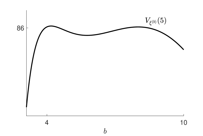
(a) $V_{{{\xi}}^{(b)}}(5)$ vs $b$.

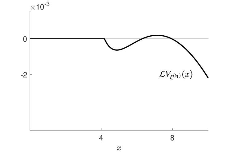
(b) ${\mathcal{L}}V_{{{\xi}}^{(b_{1})}}(x)$ vs $x$.

Figure 2. Graphs of $V_{{{\xi}}^{(b)}}(5)$ and ${\mathcal{L}}V_{{{\xi}}^{(b_{1})}}(x)$

To show that ${{{\xi}}^{(b_{1})}}$ is optimal, and not just the best barrier policy, we would need to complete the verification step. But, as Figure 2(b) shows, $V_{{{\xi}}^{(b_{1})}}(x)$ does not satisfy (22). (The same is true of $V_{{{\xi}}^{(b_{2})}}$ and $V_{{{\xi}}^{(b_{3})}}$.) We must therefore seek a new candidate for $V$.

Remark 1.

We emphasize that multiple roots of (28) does not rule out the existence of an optimal barrier policy. In fact, in most cases that we considered where (28) has three roots, the best barrier policy is optimal in ${\mathscr{A}}$ and smooth fit holds. As we have already noted, the roots of (28) are precisely the critical points of $b\mapsto V_{{{\xi}}^{(b_{1})}}$. In general, if (28) has three roots, then $b\mapsto V_{{{\xi}}^{(b_{1})}}$ has local maxima at the smallest and the largest of the three roots (compare Figure 2(a)). These maxima are related to the ‘two modes’ alluded to above.

Remark 2.

Liu et al [24] show that (28) has at most one root if $e^{\gamma_{-}-\gamma_{+}}<-\gamma_{+}/\gamma_{-}$. They also show that this equation has at most three roots. We have not been able to find a yield function (satisfying 1) for which the corresponding equation (27) has more than three roots.

5. Completing the proof of Theorem 1

Let $\eta$ be the function in (6), and let $\mu,\sigma$ and $r$ be as in (29). We aim to show that the optimal policy has action region $\mathcal{A}=[b_{1},\theta]\cup[\lambda,\infty)$, where $b_{1}$ is the smallest of the three roots of the equation (28) for a smooth fit. In view of (17), we define our candidate for $V$ as

$$v(x)=\begin{cases}A(\frac{e^{\gamma_{+}x}}{\gamma_{+}}-\frac{e^{\gamma_{-}x}}{\gamma_{-}}),\;&x\in[0,b_{1}],\\ B+\int_{b_{1}}^{x}\eta_{0}(u)du,\;&x\in(b_{1},\theta],\\ C_{1}e^{\gamma_{+}x}+C_{2}e^{\gamma_{-}x},\;&x\in(\theta,\lambda],\\ D+\int_{\lambda}^{x}\eta_{0}(u)du,\;&x\in(\lambda,\infty).\\ \end{cases}$$ (31)

Here, $A$ and $B$ are defined by $b_{1}$ and the relations (25). We let the remaining five constants $(C_{1},C_{2},D,\theta$ and $\lambda)$ be determined by $C^{2}$-smoothness at $x=\lambda$ and $C^{1}$-smoothness at $x=\theta$. These smoothness requirements lead to the equations

$$C_{1}e^{\gamma_{+}\theta}+C_{2}e^{\gamma_{-}\theta}-(B+\theta-b_{1}-\log(\theta/b_{1})) =0,$$

$$C_{1}\gamma_{+}e^{\gamma_{+}\theta}+C_{2}\gamma_{-}e^{\gamma_{-}\theta}-(1-1/\theta) =0,$$

$$C_{1}e^{\gamma_{+}\lambda}+C_{2}e^{\gamma_{-}\lambda}-D =0,$$ (32)

$$C_{1}\gamma_{+}e^{\gamma_{+}\lambda}+C_{2}\gamma_{-}e^{\gamma_{-}\lambda}-(1-\frac{1}{\lambda}) =0,$$

$$C_{1}\gamma_{+}^{2}e^{\gamma_{+}\lambda}+C_{2}\gamma_{-}^{2}e^{\gamma_{-}\lambda}-\frac{1}{\lambda^{2}} =0.$$

To verify that $V$ is indeed on the form (31), we must first specify (31), that is,

(i) provide a positive solution $$(C_{1},C_{2},D,\theta,\lambda) b_{1}<\theta<\lambda$$ to (32) with ,

and then

(ii) verify the inequalities (22) when (31) is specified by $$(b_{1},C_{1},C_{2},D,\theta,\lambda)$$. (33)

We only found one positive solution to (32) with $b_{1}<\theta<\lambda$:

$$(C_{1},C_{2},D,\theta,\lambda)\approx(0.817,\,1.58,\,0.885,\,4.84,\,7.95).$$ (34)

Now use this solution to define $v^{\ast}$ according to (31), and let ${{\xi}}^{\ast}$ be the singular policy with action region $\mathcal{A}=[b_{1},\theta]\cup[\lambda,\infty)$. Then $v^{\ast}$ meets the requirements in Lemma 1 and satisfies (17), so $Y^{v^{\ast},{{\xi}}^{\ast}}$ is a martingale. Conclude that $v^{\ast}=V_{{{\xi}}^{\ast}}$.

Turning to the verification step, Figure 3 displays the graphs of ${\mathcal{L}}v^{\ast}$ and ${\mathcal{M}}v^{\ast}$. (The discontinuity of ${\mathcal{L}}v^{\ast}$ at $x=\theta$ is a consequence of the discontinuity of the second derivative of $v^{\ast}$ at $x=\theta$.) We see that the inequalities in (22) do hold. Since $v^{\ast}$ satisfies the conditions in Lemma 2, this means that $v^{\ast}(x)\geq V(x)$, for all $x\geq 0$. We can now conclude that $v^{\ast}=V$, so that ${{\xi}}^{\ast}$ is optimal, and the proof of Theorem 1 is therefore complete.

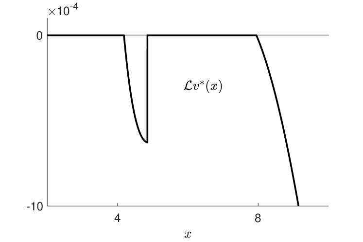
(a) ${\mathcal{L}}v^{\ast}$

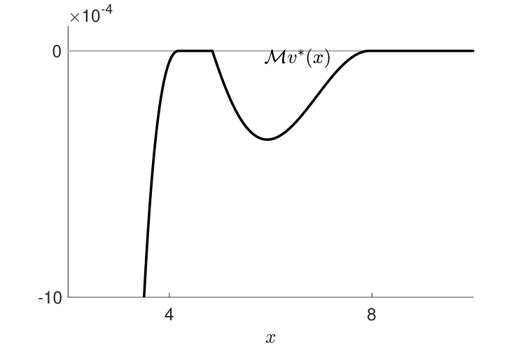
(b) ${\mathcal{M}}v^{\ast}$

Figure 3. Graphs of ${\mathcal{L}}v^{\ast}$ and ${\mathcal{M}}v^{\ast}$.

Remark 3.

We have not rigorously proved that (28) and (32) have solutions with the properties in (i)-(ii). However, it is easy to check that such a solution exists (see footnote 3). The difficult part of the proof was coming up with the correct guess that $V$ is merely once continuously differentiable at $\theta$. Here we have borrowed heavily from [24], where this result is conjectured without a verification argument for non-$C^{2}$-functions.

Remark 4.

Note that the agent makes at most one switch between $\lambda$ and $b_{1}$ when ${{\xi}}^{\ast}$ is used: once $X$ drops to $\theta$, a barrier is enforced at $b_{1}$. In the terminology of [7], $\theta$ is ‘repelling’ for the optimally controlled process. It is worth noting that the breakdown of smooth fit at the repelling boundary is consistent with [9, 10]. In retrospect, the mere $C^{1}$-smoothness of $V$ at $\theta$ is also in agreement with [7]. Indeed, the solution to our problem may be viewed as the solution to a problem involving control and stopping, where $\theta$ is the optimal stopping boundary.

Remark 5.

In the case (29) that we considered, the form of the optimal policy is quite sensitive to perturbations of the parameters. If $\mu$ is slightly decreased, then (28) has a unique solution $b\approx 4$ and (it turns out) the optimal policy is a barrier at this threshold. If $\mu$ is slightly increased, the optimal policy is a barrier at $b\approx 8$. (In view of this and the continuity of $v^{\ast}$, it should come as no surprise that the advantage of using ${{\xi}}^{\ast}$ over ${{{\xi}}^{(b_{1})}}$ is less than $0.01\,\%$.) Informally, the phenomenon that we have encountered arises on the boundary between two parts of the parameter space on which the optimal policies have distinct qualitative properties. We elaborate this interpretation in the next and final section of the paper.

Remark 6.

The phenomenon that we have encountered does not arise in the absence of reflection (i.e., if the reflection process ${\mathscr{L}}$ is removed from (1)). The analysis of this much simpler problem is similar to that of the problem that we have studied, but the condition $v^{\prime}(0)=0$ is no longer needed to ensure that (12) is a martingale. For any $\eta$ satisfying 1, the value of ${{\xi}}^{(b)}$ is given by (compare (25))

$$\widetilde{V}_{{{\xi}}^{(b)}}(x)=\begin{cases}&\gamma_{+}^{-1}\eta(b)\cdot e^{\gamma_{+}(x-b)},\quad x\in(-\infty,b],\\ &\gamma_{+}^{-1}\eta(b)+\int_{b}^{x}\eta(u)du,\quad x\in(b,\infty).\end{cases}$$ (35)

Smooth ($C^{2}$) fit at $x=b$ leads to the equation

$$\gamma_{+}\cdot\eta(b)=\eta^{\prime}(b).$$ (36)

By 1(i), the function $b\mapsto\gamma_{+}\eta(b)-\eta^{\prime}(b)$ is strictly increasing on $(0,\infty)$, so (36) has a unique solution $b^{\ast}\in(0,\infty)$. Using concavity of $\eta$, it is not difficult to prove that ${{\xi}}^{(b^{\ast})}$ is optimal in $\mathscr{A}$ (see [21]). Hence, in the absence of reflection, the value function is of class $C^{2}$ and there is always an optimal barrier policy.

6. Final remarks on the optimal policy

It remains to address the question of whether the phenomenon portrayed in Figure 1 should be viewed as a flaw of the reflected Brownian model (1) in applications of the type that we have mentioned. We will suggest that this phenomenon does in fact correspond to observed behavior, for which the model may thus provide a rational explanation. This interpretation should be compared with Henderson and Hobson’s [19] interpretation of a phenomenon which at first appears similarly puzzling.

Let us first note that although the band policy that we have encountered appears to be a new phenomenon, policies involving multiple thresholds are well known to arise in some problems of optimal control. One such problem is the stochastic cash balance problem studied by Harrison et al [18] in which the contents of a cash fund can be decreased or increased at proportional plus fixed costs. Under optimal control, the fund’s manager effectuates an upward jump to $q>0$ each time $0$ is hit, and a downward jump to $Q>q$ whenever the contents process reaches $S>Q$. As noted in [18], this form of the optimal policy is easily anticipated in view of the fixed transaction costs. When these costs tend to $0$, the optimal policy enforces a single upper barrier. The band structure of the optimal policy is thus a consequence of features of the problem that are not present in our model.

The band policy portrayed in Figure 1 is best understood as a switch between two modes of operation. The modes in question are related to local maxima of $b\mapsto V_{{{\xi}}^{(b)}}$. As previously noted (see Remark 1), this function has two local maxima if the equation (28) for a smooth fit has three roots, the maxima occurring at the smallest and the largest root. These roots may be thought of as providing the best representatives from each of two qualitatively different types of barrier policies. Policies of the first type exert control where marginal yield is high. These policies are risky in the sense that there may be long time intervals during which no yield is accumulated. The second type of policies accumulate yield closer to the origin and are therefore less risky in this sense. In the case (29) that we have studied, the optimal policy has an interesting interpretation: The risk-neutral decision maker initially gambles on the more risky strategy, but lowers risk if this strategy underperforms.

Such behavior can be observed in roughly the following situation: An agent may choose between two plans, $A$ and $B$, where $A$ has the potential of yielding high marginal reward while $B$ offers lower marginal reward at lower risk. Here, the idea of falling back on B if A underperforms is quite familiar. Our results suggest that such behavior can align with risk-neutral preferences if the expected reward of choosing A is close to that of choosing B. Additionally, the expected reward of choosing A should be smaller than that of choosing B; an expectation-maximizing agent would not have an incentive to abandon A if the opposite were true.

Acknowledgement

The problem dealt with in this paper was presented to me by Larry Shepp on my arrival to Rutgers University as a visiting student from KTH on July 5th, 2003. I am grateful for that highly stimulating summer, during which some of the results presented in this paper were obtained. I am also grateful to Naomi Zeitouni and Ofer Zeitouni for helpful discussions, in 2003 and in 2023.

References

- [1] Luis H. R. Alvarez. Singular stochastic control in the presence of a state-dependent yield structure. Stochastic processes and their applications, 86:323–343, 2000.
- [2] Luis H. R. Alvarez and Larry A. Shepp. Optimal harvesting of stochastically fluctuating populations. Journal of Mathematical Biology, 37:155–177, 1998.
- [3] F. A. Attia and P. J. Brockwell. The control of a finite dam. Journal of Applied Probability, 19(4):815–825, 1982.
- [4] Václav E. B., L. A. Shepp, and H. S. Witsenhausen. Some solvable stochastic control problems. Stochastics, 4(1):39–83, 1980.
- [5] John Bather and Herman Chernoff. Sequential decisions in the control of a space-ship (finite fuel). Journal of Applied Probability, 4(3):584–604, 1967.
- [6] M. Chaleyat-Maurel, N. El Karoui, and B. Marchal. Reflexion discontinue et systemes stochastiques. The annals of probability, 8(6):1049–1067, 1980.
- [7] M. H. A. Davis and M. A. Zervos. A problem of singular stochastic control with discretionary stopping. The Annals of Applied Probability, 4(1):226–240, 1994.
- [8] M. H. A. Davis and M. A. Zervos. A pair of explicitly solvable singular stochastic control problems. Applied Mathematics and Optimization, 38:327–352, 1998.
- [9] Tiziano De Angelis, Giorgio Ferrari, and John Moriarty. A nonconvex singular stochastic control problem and its related optimal stopping boundaries. SIAM Journal on Control and Optimization, 53(3):1199–1223, 2015.
- [10] Tiziano De Angelis, Giorgio Ferrari, and John Moriarty. A solvable two-dimensional degenerate singular stochastic control problem with nonconvex costs. Mathematics of Operations Research, 44(2):512–531, 2018.
- [11] Julia Eisenberg and Paul Krüner. On Itô’s formula for semimartingales with jumps and non- functions. Statistics and Probability Letters, 184:109369, 2022.
- [12] Julia Eisenberg and Hanspeter Schmidli. Discontinuous reflection, and a class of singular stochastic control problems for diffusions. Journal of Applied Probability, 4(3):733–748, 2011.
- [13] Nicole El Karoui and Ioannis Karatzas. Probabilistic aspects of finite-fuel, reflected follower problems. Acta Applicandae Mathematica, 11(3):223–258, 1988.
- [14] Giorgio Ferrari. On a class of singular stochastic control problems for reflected diffusions. Journal of Mathematical Analysis and Applications, 473:952–979, 2019.
- [15] Giorgio Ferrari and Patrick Schuhmann. An optimal dividend problem with capital injections over a finite horizon. SIAM Journal on Control and Optimization, 57(4):2686–2719, 2019.
- [16] Xin Guo and Pascal Tomecek. A class of singular control problems and the smooth fit principle. SIAM Journal on Control and Optimization, 47(6):3076–3099, 2009.
- [17] Xin Guo and Guoliang Wu. A class of singular control problems and the smooth fit principle. SIAM Journal on Control and Optimization, 48(2):594–617, 2009.
- [18] Michael J. Harrison, Thomas M. Sellke, and Allison J. Taylor. Impulse control of brownian motion. Mathematics of Operations Research, 8(3):454–466, 1983.
- [19] Vicky Henderson and David Hobson. An explicit solution for an optimal stopping/optimal control problem which models an asset sale. The Annals of Applied Probability, 18(5):1681–1705, 2008.
- [20] Andrew Jack, Timothy C. Johnson, and Mihail A. Zervos. A singular control model with application to the goodwill problem. Journal of Applied Probability, 118:2098–2124, 2008.
- [21] Adam Jonsson Oduya. Explicit solutions to a pair of continuous time stochastic control problems. PhD thesis, Rutgers University, 2008.
- [22] Ioannis Karatzas. A class of singular stochastic control problems. Advances in Applied Probability, 15(2):225–254, 1983.
- [23] Ioannis Karatzas and Steven E. Shreve. Connections between optimal stopping and singular stochastic control II. reflected follower problems. SIAM Journal on Control and Optimization, 86(3):443–451, 1968.
- [24] Jun Liu, Ben Logan, Eric Shepp, Lawrence A. Shepp, Naomi Zeitouni, and Ofer Zeitouni. Optimal pumping may be anomalous, 2003. manuscript.
- [25] Arne Løkka and Mihail Zervos. Optimal dividend and issuance of equity policies in the presence of proportional costs. Insurance: Mathematics and Economics, 42(3):954–961, 2008.
- [26] Pui Chan Lon and Mihail Zervos. A model for optimally advertising and launching a product. Mathematics of Operations Research, 36(2):363–376, 2011.
- [27] H. P. McKean and L. A. Shepp. The advantage of capitalism vs. socialism depends on the criterion. Zapiski Nauchnykh Seminarov POMI, 328:160–168, 2005.
- [28] Goran Peskir. Principle of smooth fit and diffusions with angles. Stochastics, 79(3-4):293–302, 2007.
- [29] Evan L. Porteus. On optimal dividend, reinvestment, and liquidation policies for the firm. Operations Research, 25(5):818–834, 1977.
- [30] Philip E. Protter. Stochastic Integration and Differential Equations. Stochastic Modelling and Applied Probability. Springer, 2005.
- [31] Roy Radner and Larry Shepp. Risk vs. profit-potential: A model for corporate strategy. Journal of Economic Dynamics and Control, 20(8):1373–1393, 1996.
- [32] S. E. Shreve, J. P. Lehoczky, and D. P. Gaver. Optimal consumption for general diffusions with absorbing and reflecting barriers. SIAM Journal on Control and Optimization, 22(1):55–75, 1984.
- [33] Ky Q. Tran, Bich T. N. Le, and George Yin. Harvesting of a stochastic population under a mixed regular-singular control formulation. Journal of Optimization Theory and Applications, 195(3):1106–1132, 2022.
- [34] Lam Yeh. Optimal control of a finite dam: Average-cost case. Journal of Applied Probability, 22(2):480–404, 1985.
- [35] Naomi Zeitouni. Optimal extraction from a renewable groundwater aquifer with stochastic recharge. Water Resources Research, 40(6):1–8, 2004.
- [36] Hang Zhu. Generalized solution in singular stochastic control: The nondegenerate problem. Applied Mathematics and Optimization, 25:225–245, 1992.
- [37] Jinxia Zhu and Hailiang Yang. Optimal capital injection and dividend distribution for growth restricted diffusion models with bankruptcy. Insurance: Mathematics and Economics, 70(2):259–271, 2016.