Renormalized Primordial Black Holes

G. Franciolini,¹ A. Ianniccari,² A. Kehagias, ^2,3 D. Perrone,² and A. Riotto,²

¹ CERN, Theoretical Physics Department, Esplanade des Particules 1, Geneva 1211, Switzerland

² Department of Theoretical Physics and Gravitational Wave Science Center (GWSC),
Université de Genève, CH-1211 Geneva

³ Physics Division, National Technical University of Athens, Athens, 15780, Greece

  Abstract
The formation of primordial black holes in the early universe may happen through the collapse of large curvature perturbations generated during a non-attractor phase of inflation or through a curvaton-like dynamics after inflation. The fact that such small-scale curvature perturbation is typically non-Gaussian leads to the renormalization of composite operators built up from the smoothed density contrast and entering in the calculation of the primordial black abundance. Such renormalization causes the phenomenon of operator mixing and the appearance of an infinite tower of local, non-local and higher-derivative operators as well as to a sizable shift in the threshold for primordial black hole formation. This hints that the calculation of the primordial black hole abundance is more involved than what generally assumed.

 

1 Introduction

The physics of Primordial Black Holes (PBHs) [1, 2, 3, 4] has recently attracted much attention thanks to the plethora of gravitational wave detections from the mergers of BH binaries [5, 6, 7, 8]. Maybe even more interesting, some of the LIGO/Virgo/KAGRA events might be in fact originating from the mergers of PBHs [9, 10, 11, 12, 13, 14, 15, 16]. Future gravitational wave experiments might help in shedding light on the possible existence of PBHs [17, 18, 19, 20, 21].

In this paper we will start from the rather standard point of view that PBHs are born in the radiation-dominated era by the collapse of large overdensities generated on small scales during a non-attractor phase of inflation or through a curvaton-like dynamics after inflation  [1].

Calculating the abundance of PBHs as precisely as possible is a crucial step in assessing if PBHs may account for a substantial fraction of the dark matter of the universe or if they satisfy the different observational constraints. Such computation is rendered difficult as PBHs are rare events and therefore the formation probability is sensitive to small changes in the various ingredients, such as the critical threshold of collapse [22, 23], the non-Gaussian nature of the fluctuations [24, 25], the choice of the window function to define smoothed observables [26], to mention a few. Furthermore it has been recently pointed out that non-linear corrections entering in the calculation of the PBHs abundance from the non-linear radiation transfer function and the determination of the true physical horizon crossing corrects the overdensity (on comoving orthogonal slices) by introducing many non-linear terms, even of non-local type [27]. This makes the calculation of the formation probability highly nontrivial.

In this paper we point out that the standard way of calculating the PBH abundance, which we will revise in the next section, overlooks a technical, but simple point. In the standard calculation one defines a smoothed density contrast $\delta_{m}(r_{m},\vec{x}_{\rm pk})$, which depends on the position $\vec{x}_{\rm pk}$ of the peak of the profile of the overdensity and on the distance $r_{m}$ from it where the compaction function has its maximum. This field turns out to be the sum of a field $\delta(r_{m},\vec{x}_{\rm pk})$, but also its square $\delta^{2}(r_{m},\vec{x}_{\rm pk})$. The latter is a composite operator, i.e., evaluated at the same point of space (and time), and receives loop contributions from all scales. This happens because $\delta(r_{m},\vec{x}_{\rm pk})$ is proportional to the gradient of the small-scale curvature perturbation and the latter is typically non-Gaussian (see e.g., [28]). In other words the curvature perturbation has cubic and quartic interactions, leading to the renormalization of the composite operator $\delta^{2}(r_{m},\vec{x}_{\rm pk})$ and therefore of $\delta_{m}(r_{m},\vec{x}_{\rm pk})$.

The renormalization procedure leads to the well-known phenomenon of operator mixing: the renormalized operator $\delta^{2}(r_{m},\vec{x}_{\rm pk})$ receives corrections from all possible operators compatible with the symmetries of the problem. We will show that indeed one-loop corrections assume the form of an infinite tower of operators, even non-local in $\delta(r_{m},\vec{x}_{\rm pk})$ and of the higher-derivative type. It is the interacting nature of the comoving curvature perturbation which gives rise to the phenomenon of operator mixing, which leads to a shift in the correlators and the threshold for PBH formation, as well as a modification of the formation probability.

The paper is organized as follows. In section 2 we set the stage and describe briefly the standard way of calculating the PBH abundance. In section 3 we remind the reader why PBH formation models are characterized by a non-Gaussian curvature perturbation. In section 4 we introduce the concept of renormalization of the PBHs and the Feynman rules we will adopt to calculate the operator mixing at one-loop, which we do in sections 5 and 6. Section 7 contains our conclusions, while we devote the appendices A and B to the technical details.

2 A brief summary of the standard PBH abundance calculation

The goal of this section is to set the stage and briefly recap what is the standard procedure to calculate the PBH abundance in the literature, see for instance Refs. [25, 29].

As we already wrote, our focus will be the PBH formation from the collapse of large overdensities which are generated during inflation and re-enter the Hubble radius in the radiation-dominated era. The key starting object is the curvature perturbation $\zeta$ appearing in the metric in the comoving uniform-energy density gauge

$${\rm d}s^{2}=-{\rm d}t^{2}+a^{2}(t)e^{2\zeta(\vec{x})}{\rm d}{\vec{x}}^{2}.$$ (2.1)

Here $a(t)$ is the scale factor in terms of the cosmic time. Applying the gradient expansion on superhoizon scales  [30], one can relate the non-linear density contrast $\delta_{\rm com}(\vec{x},t)$ on comoving orthogonal slicings and the time independent curvature perturbation $\zeta(\vec{x})$  [31]

$$\delta_{\rm com}(\vec{x},t)=-\frac{8}{9}\frac{1}{a^{2}H^{2}}e^{-5\zeta(\vec{x})/2}\nabla^{2}e^{\zeta(\vec{x})/2},$$ (2.2)

where $H$ is the Hubble rate. Cosmological perturbations may gravitationally collapse to form a PBH depending upon the amplitude measured at the peak of the compaction function, defined to be the mass excess compared to the background value in a given radius [31, 22, 32]. On superhorizon scales and assuming spherical symmetry, it reads

$$\mathcal{C}(r)=-\frac{2}{3}r\partial_{r}\zeta(r)\left[2+r\partial_{r}\zeta(r)\right].$$ (2.3)

The compaction function has a maximum at the comoving length scale $r_{m}$ such that

$$\left.\partial_{r}\zeta(r)+r_{m}\partial_{r}^{2}\zeta(r)\right|_{r=r_{m}}=0,$$ (2.4)

and one can define a smoothed perturbation amplitude as the volume average of the energy density contrast within the scale $r_{m}$ at the Hubble radius crossing time $t_{H}$ [22]

$$\delta_{m}=\frac{3}{\left(r_{m}e^{\zeta(r_{m})}\right)^{3}}\int_{0}^{r_{m}}{\rm d}r\,\delta_{\rm com}(r,t_{H})\left(re^{\zeta(r)}\right)^{2}\partial_{r}\left(re^{\zeta(r)}\right),$$ (2.5)

where a top-hat window function needs to be used for a proper treatment of the threshold [26].

The quantity $\delta_{m}$ is crucial in determining the abundance of PBHs. If computed at the Hubble radius crossing time $t_{H}$, that is

$$\epsilon(t_{H})=\frac{r_{H}}{r_{m}e^{\zeta(r_{m})}}=\frac{1}{r_{m}e^{\zeta(r_{m})}\,aH}=1,$$ (2.6)

it becomes

$$\delta_{m}=\delta_{l}-\frac{3}{8}\delta_{l}^{2},\qquad\delta_{l}=-\frac{4}{3}r_{m}\left.\partial_{r}\zeta(r)\right|_{r=r_{m}}.$$ (2.7)

The PBH abundance is subsequently calculated integrating the probability distribution function of the smoothed density contrast from a threshold value $\delta_{c}$ on

$$\beta=\int_{\delta_{c}}{\rm d}\delta_{m}\left(\frac{M_{\rm PBH}}{M_{H}}\right)P(\delta_{m}),$$ (2.8)

as a function of the PBH mass $M_{\rm PBH}$ and the mass $M_{H}$ enclosed in the Hubble volume. One can then use the conservation of probability to write [33, 25, 29, 34, 28, 35]

$$P(\delta_{l}){\rm d}\delta_{l}=P(\delta_{m}){\rm d}\delta_{m},$$ (2.9)

with threshold given by [25]

$$\delta_{l,c}=\frac{4}{3}\left(1-\sqrt{1-\frac{3}{2}\delta_{c}}\right),$$ (2.10)

where $\delta_{c}$ is the threshold routinely computed by running numerical simulations [22].

For Gaussian curvature perturbations, the probability of the linear density contrast is Gaussian and is exponentially sensitive to the threshold $\delta_{l,c}$ and the variance $\sigma^{2}_{l}$

$$P(\delta_{l}) =\frac{1}{\sqrt{2\pi}\sigma_{l}}e^{-\delta_{l}^{2}/2\sigma_{l}^{2}},$$

$$\sigma_{l}^{2} =\int\frac{{\rm d}k}{k}{\cal P}_{\delta_{l}}(k),$$ (2.11)

where ${\cal P}_{\delta_{l}}$ is the dimensionless power spectrum of the density contrast $\delta_{l}$.

3 The non-Gaussianity of the curvature perturbation

The probability (2) is valid only if the smoothed density contrast $\delta_{l}$ is linear (hence the _l subscript). Given the relation

$$\delta_{l}(r_{m})=-\frac{4}{3}r_{m}\left.\partial_{r}\zeta(r)\right|_{r=r_{m}},$$ (3.1)

one concludes that $\delta_{l}$ is indeed linear only if the curvature perturbation is linear. However, in all models in which a large fluctuation in the curvature perturbation is generated, the curvature perturbation is typically non-Gaussian (see, for instance, Ref. [28]). Non-Gaussianity among the modes interested in the growth of the curvature perturbation is generated either by their self-interaction during the ultra slow-roll phase [38] or after Hubble radius exit when the curvature perturbation is sourced by a curvaton-like field [39, 40].

Even though in general the exact relation between $\zeta$ and its corresponding Gaussian component $\zeta_{g}$ can be worked out model by model, we will adopt a cubic expansion to be model independent,

$$\zeta=\zeta_{g}+\frac{3}{5}f_{NL}\zeta_{g}^{2}+\frac{9}{25}g_{NL}\zeta_{g}^{3},$$ (3.2)

which is a good approximation if $(3/5)f_{NL}\zeta_{g}$ and $(9/25)g_{NL}\zeta^{2}_{g}\mathrel{\hbox to0.0pt{\lower 4.0pt\hbox{\hskip 0.5pt$\sim$}\hss}\raise 1.0pt\hbox{$<$}}1$. For instance, in models with a sharp transition between the ultra slow-roll phase and the subsequent slow-roll phase one has $f_{NL}\simeq 5/2$ and $g_{NL}\simeq 25/6$ (see, for instance, Ref. [38]) and therefore the expansion is motivated as long as $\zeta_{g}\mathrel{\hbox to0.0pt{\lower 4.0pt\hbox{\hskip 0.5pt$\sim$}\hss}\raise 1.0pt\hbox{$<$}}0.7$. The expansion is also justified if we perform a perturbative loop expansion and think the non-Gaussianity as leading to three-, four-point vertices, and so on.

The non-Gaussianity of the curvature perturbation is crucial in changing the PBH abundance. Indeed, around peaks of the power spectrum of the curvature perturbation, a positive $f_{NL}$ increases the abundance of the PBHs, while a negative $f_{NL}$ has the opposite effect, thus helping to interpret the recent pulsar timing array observation of a stochastic gravitational wave background [41, 42, 43, 44, 45, 46, 47, 48, 49] by using the scalar-induced gravitational waves sourced along with PBH formation [50, 51, 52, 53, 54, 55, 56, 57, 58].

The importance of the non-Gaussianity in the curvature perturbation will become clear in the following section, where we will go back to the smoothed density contrast $\delta_{m}$ and deal with the fact that it is a composite operator.

4 Renormalization in the PBHs

We start again from the expression (2.7) of the smoothed density contrast

$$\delta_{m}(r_{m},\vec{x}_{\rm pk})=\frac{3}{4\pi r_{m}^{3}}\int{\rm d}^{3}x\,\delta_{\rm com}(\vec{x},t_{H})\,\theta(r_{m}-|\vec{x}-\vec{x}_{\rm pk}|)=\delta(r_{m},\vec{x}_{\rm pk})-\frac{3}{8}\delta^{2}(r_{m},\vec{x}_{\rm pk}),$$ (4.1)

where this time we removed the subscript _l to account for the fact that $\delta_{l}$ is not a Gaussian field, since the curvature perturbation is not. Furthermore we have highlighted the fact that $\delta_{m}$ depends on the peak position $\vec{x}_{\rm pk}$ and from the distance $r_{m}$ from the peak.

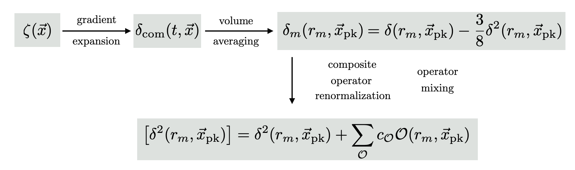
Figure 1: Schematic view of operations the leading to the composite operator renormalization.

The key point is that $\delta_{m}(r_{m},\vec{x}_{\rm pk})$ contains the composite operator $\delta^{2}(r_{m},\vec{x}_{\rm pk})$ which receives contributions from all scales, not only from the infrared ones. This is because two small-scale modes may combine in the loops to form a long mode. Such contributions may be therefore not small at all, even on large scales. One should also recall at this stage that, even in the presence of the window function cutting-off ultraviolet momenta, variances are typically dominated by integrating momenta corresponding to length scales well beneath the horizon [27].

One needs to renormalize the composite operator $\delta^{2}(r_{m},\vec{x}_{\rm pk})$ at the point $\vec{x}_{\rm pk}$ in such a way that all potentially large contributions can be systematically removed by adding local counterterms (canceling as well the dependence on an unphysical cut-off scale, if needed)

$$\left[\delta^{2}(r_{m},\vec{x}_{\rm pk})\right]\equiv\delta^{2}(r_{m},\vec{x}_{\rm pk})+\sum_{\cal O}c_{\cal O}{\cal O}(r_{m},\vec{x}_{\rm pk}),$$ (4.2)

where the square brackets indicate the renormalized operator. This means that the renormalized composite operator will mix with possibly all the other operators ${\cal O}(r_{m},\vec{x}_{\rm pk})$ which are allowed by the symmetries of the problem. It will also have an impact on the PBH abundance, being it so sensitive to minute changes in the threshold and/or in the variances.

The goal of the subsequent sections is to perform the systematic renormalization of the smoothed density contrast.

4.1 Feynman rules

Our starting point is the expression

$$\delta(r_{m},\vec{x}_{\rm pk})=-\frac{4}{3}r\partial_{r}\zeta(r_{m},\vec{x}_{\rm pk})=-\frac{4}{9}\int\frac{{\rm d}^{3}k}{(2\pi)^{3}}\;e^{i\vec{k}\cdot\vec{x}_{\rm pk}}k^{2}r_{m}^{2}W_{3}(kr_{m})\zeta_{\vec{k}},$$ (4.3)

whose Fourier transform reads

$$\delta_{\vec{k}}(r_{m})=-\frac{4}{9}k^{2}r_{m}^{2}W_{3}(kr_{m})\zeta_{\vec{k}}.$$ (4.4)

Here $W_{3}(kr_{m}$) is the Fourier transform of the top-hat window function in real space with radius $r_{m}$

$$W_{3}(x)=3\frac{\sin x-x\cos x}{x^{3}}=2^{3/2}\Gamma(5/2)\frac{J_{3/2}(x)}{x^{3/2}},$$ (4.5)

being $J_{\nu}(x)$ the Bessel function of the first kind. To simplify the notation we have absorbed the time-dependent radiation transfer function in the curvature perturbation $\zeta_{\vec{k}}$ (and in its power spectrum). All power spectra will be intended to be calculated at horizon crossing.

The renormalization of the composite operator $\delta^{2}(r_{m},\vec{x}_{\rm pk})$ will proceed through the following Feynman rules:

• draw every $N$-point connected graph and conserve momentum in each vertex;

• to each $(n+1)$ point vertex, with a solid line (in-going momentum) and $n$ dashed lines, it corresponds the following vertex

  $$=(-1)^{n-1}n!\,F_{n}\;\;\frac{(qr_{m})^{2}W_{3}(qr_{m})}{\left(\frac{4}{9}\right)^{n-1}\prod_{i=1}^{n}(q_{i}r_{m})^{2}W_{3}(q_{i}r_{m})},$$ (4.6)

  where in the numerator there is the factor $(4/9)(qr_{m})^{2}W_{3}(qr_{m})$ for the solid line and at the denominator a product of all the factors $(4/9)(q_{i}r_{m})^{2}W_{3}(q_{i}r_{m})$ for each dashed lines;

• the propagator, represented with a dashed line, corresponds to

  $$\parbox[c]{65.043pt}{\includegraphics[scale={0.9}]{Figures/D_propagator_t.pdf}}\ =P_{\delta}(q)=\frac{16}{81}r_{m}^{4}q^{4}\,W^{2}_{3}(qr_{m})P_{\zeta_{g}}(q);$$ (4.7)

• integrate for every loop

  $$\int_{\vec{q}}=\int\frac{d^{3}q}{(2\pi)^{3}};$$ (4.8)

• multiply a Dirac delta with all the external momenta, for the global momentum conservation

  $$(2\pi)^{3}\delta^{(3)}\left(\sum_{i=1}^{N}\vec{k}_{i}\right);$$ (4.9)

Here $F_{n}$ is a function that depends on the number of legs in the vertex, for example from Eq. (3.2)

$$F_{1}=1,\quad F_{2}=\frac{3}{5}f_{NL},\quad F_{3}=\frac{9}{25}g_{NL}.$$ (4.10)

Notice that for the $n=1$ vertex we have

$$\parbox[c]{56.3706pt}{\includegraphics[scale={0.9}]{Figures/D_2-point_t.pdf}}=\frac{(qr_{m})^{2}W_{3}(qr_{m})}{(q_{1}r_{m})^{2}W_{3}(q_{1}r_{m})}=1,$$ (4.11)

which is just a consequence of momentum conservation.

5 Renormalization at one-loop: linear operator mixing

By indicating the composite operator with the following vertex

$$\delta^{2}=\parbox[c]{33.9669pt}{\includegraphics[scale={0.8}]{Figures/D_composite_t.pdf}}$$ (5.1)

its expectation value is obtained from the Feynman diagram

$$\parbox[c]{37.5804pt}{\includegraphics[scale={0.8}]{Figures/D_loop_0legs_t.pdf}}\ =(2\pi)^{3}\delta^{(3)}(\vec{k})\int_{\vec{q}}P_{\delta}(q),$$ (5.2)

which gives

$$\langle\left(\delta^{2}\right)_{\vec{k}}\rangle^{\prime}=\int_{\vec{q}}P_{\delta}(q)=\frac{16}{81}r_{m}^{4}\int_{\vec{q}}q^{4}\,W^{2}_{3}(qr_{m})P_{\zeta_{g}}(q)=\sigma^{2}_{\delta(r_{m})}.$$ (5.3)

Here and in the following primes indicate that we remove the factors of $(2\pi)^{3}$ times the Dirac delta for the momentum conservation. This vacuum expectation value is removed by adding a constant counterterm

$$\left[\delta^{2}(r_{m},\vec{x}_{\rm pk})\right]=\delta^{2}(r_{m},\vec{x}_{\rm pk})-\sigma^{2}_{\delta(r_{m})}.$$ (5.4)

Subtracting this tadpole contribution ensures that the vacuum expectation value of $\delta_{m}$ vanishes at the loop level. Furthermore, in the following calculations this constant counterterm will only contribute to disconnected graphs.

The one-loop contribution to $\langle(\delta^{2})_{\vec{k}_{1}}\delta_{\vec{k}_{2}}\rangle$ is, diagramatically

$$\langle(\delta^{2})_{\vec{k}_{1}}\delta_{\vec{k}_{2}}\rangle^{\prime}=2\times\parbox[c]{37.5804pt}{\includegraphics[scale={0.8}]{Figures/D_loop_1leg_t.pdf}}\;,$$ (5.5)

which gives

$$\langle(\delta^{2})_{\vec{k}_{1}}\delta_{\vec{k}_{2}}\rangle^{\prime} = -\frac{12}{5}f_{NL}\int_{\vec{q}}\;\frac{(|\vec{k}_{1}-\vec{q}|r_{m})^{2}W_{3}(|\vec{k}_{1}-\vec{q}|r_{m})}{\frac{4}{9}(k_{2}r_{m})^{2}W_{3}(k_{2}r_{m})(qr_{m})^{2}W_{3}(qr_{m})}\;P_{\delta}(k_{2})P_{\delta}(q)$$

$$= -\frac{12}{5}\cdot\frac{4}{9}\cdot\frac{16}{81}f_{NL}\int_{\vec{q}}r_{m}^{6}q^{2}|\vec{k}_{1}-\vec{q}|^{2}k_{2}^{2}\;W_{3}\left(|\vec{k}_{1}-\vec{q}|r_{m}\right)W_{3}(k_{2}r_{m})W_{3}(qr_{m})P_{\zeta_{g}}(q)P_{\zeta_{g}}(k_{2}).$$

We now use Eq. (A.1) to perform the angular integral and obtain

$$\langle(\delta^{2})_{\vec{k}_{1}}\delta_{\vec{k}_{2}}\rangle^{\prime} = I^{(1)}_{\rm one-leg}+I^{(2)}_{\rm one-leg},$$

$$I^{(1)}_{\rm one-leg} = -\frac{256}{1215}f_{NL}\int_{\vec{q}}r_{m}^{6}q^{2}(q^{2}+k_{2}^{2})k_{2}^{2}\;W_{3}^{2}(k_{2}r_{m})W^{2}_{3}(qr_{m})P_{\zeta_{g}}(q)P_{\zeta_{g}}(k_{2})$$

$$I^{(2)}_{\rm one-leg} = -\frac{256}{1215}f_{NL}\int_{\vec{q}}r_{m}^{6}q^{2}k_{2}^{2}\;W^{2}_{3}(k_{2}r_{m})W^{2}_{3}(qr_{m})\left(\frac{q^{2}}{3}\frac{{\rm d}\ln W_{3}(k_{2}r_{m})}{{\rm d}\ln k_{2}r_{m}}+\;\frac{k_{2}^{2}}{3}\frac{{\rm d}\ln W_{3}(qr_{m})}{{\rm d}\ln qr_{m}}\right)$$

$$\cdot P_{\zeta_{g}}(q)P_{\zeta_{g}}(k_{2})\;.$$

The first integral gives

$$I^{(1)}_{\rm one-leg}=\frac{12}{5}f_{NL}\left(\sigma^{2}_{\delta(r_{m})}\langle\zeta_{g\vec{k}_{1}}(r_{m})\delta_{\vec{k}_{2}}(r_{m})\rangle^{\prime}+\frac{4}{9}\sigma^{2}_{\nabla\zeta_{g}(r_{m})}\langle\delta_{\vec{k}_{1}}(r_{m})\delta_{\vec{k}_{2}}(r_{m})\rangle^{\prime}\right),$$ (5.8)

where

$$\zeta_{g}(r_{m},\vec{x}_{\rm pk})=\int\frac{{\rm d}^{3}k}{(2\pi)^{3}}\,e^{i\vec{k}\cdot\vec{x}_{\rm pk}}\zeta_{g\vec{k}}(r_{m})=\int\frac{{\rm d}^{3}k}{(2\pi)^{3}}\,e^{i\vec{k}\cdot\vec{x}_{\rm pk}}W_{3}(kr_{m})\zeta_{g\vec{k}}$$ (5.9)

and

$$\sigma^{2}_{\nabla\zeta_{g}(r_{m})}=\int_{\vec{q}}r_{m}^{2}q^{2}W_{3}^{2}(qr_{m})P_{\zeta_{g}}(q).$$ (5.10)

The second integral gives

$$I^{(2)}_{\rm one-leg}=\frac{12}{5}f_{NL}\left[\frac{1}{3}\sigma^{2}_{\delta(r_{m})}\frac{{\rm d}}{{\rm d}\ln r_{m}}\langle\zeta_{g\vec{k}_{1}}(r_{m})\delta_{\vec{k}_{2}}(r_{m})\rangle^{\prime}+\frac{4}{9}\cdot\left(\frac{1}{6}\frac{{\rm d}\sigma^{2}_{\nabla\zeta_{g}(r_{m})}}{{\rm d}\ln r_{m}}-\frac{1}{3}\sigma^{2}_{\nabla\zeta_{g}(r_{m})}\right)\langle\delta_{\vec{k}_{1}}\delta_{\vec{k}_{2}}\rangle^{\prime}\right].$$

Therefore, the renormalized operator at the level of linear mixing becomes (see Appendix B)

$\displaystyle\left[\delta^{2}(r_{m},\vec{x}_{\rm pk})\right]_{\text{linear }}$ $\displaystyle=$ $\displaystyle\delta^{2}(r_{m},\vec{x}_{\rm pk})-\sigma^{2}_{\delta(r_{m})}-\frac{12}{5}f_{NL}\cdot\frac{4}{9}\left(\frac{2}{3}\sigma^{2}_{\nabla\zeta_{g}(r_{m})}+\frac{1}{6}\frac{{\rm d}\sigma^{2}_{\nabla\zeta_{g}(r_{m})}}{{\rm d}\ln r_{m}}\right)\delta(r_{m},\vec{x}_{\rm pk})$ $\displaystyle+$ $\displaystyle\frac{12}{5}f_{NL}\cdot\frac{5}{3}\cdot\sigma^{2}_{\delta(r_{m})}\zeta(r_{m},\vec{x}_{\rm pk}),$

$$= \hskip 14.22636pt\parbox[c]{37.5804pt}{\includegraphics[scale={0.8}]{Figures/D_loop_1leg_t.pdf}}\hskip 14.22636pt+\hskip 14.22636pt\parbox[c]{6.5043pt}{\includegraphics[scale={1}]{Figures/D_counter1_t.pdf}}$$ (5.12)

where we have added the corresponding Feynman diagram for the counterterm. We see that already at this level there appears a non-local operator in the density smoothed contrast field $\delta(r_{m},\vec{x}_{\rm pk})$ once the following identity

$$\zeta_{g}(r_{m},\vec{x}_{\rm pk})=\frac{9}{4r_{m}^{2}\nabla^{2}_{x_{\rm pk}}}\delta(r_{m},\vec{x}_{\rm pk})$$ (5.13)

is adopted.

6 Renormalization at one-loop: quadratic operator mixing

The one-loop contribution to $\langle[\delta^{2}]_{\vec{k}_{1}}\delta_{\vec{k}_{2}}\delta_{\vec{k}_{3}}\rangle$ is diagramatically

$$\langle[\delta^{2}]_{\vec{k}_{1}}\delta_{\vec{k}_{2}}\delta_{\vec{k}_{3}}\rangle^{\prime}\hskip 8.5359pt=\hskip 8.5359pt\parbox[c]{37.5804pt}{\includegraphics[scale={0.8}]{Figures/D_loop_2legs_1_t.pdf}}\hskip 8.5359pt+\hskip 8.5359pt2\times\parbox[c]{47.6982pt}{\includegraphics[scale={0.8}]{Figures/D_loop_2legs_2_t.pdf}}\hskip 8.5359pt+\hskip 8.5359pt\parbox[c]{27.4626pt}{\includegraphics[scale={0.85}]{Figures/D_counter2_t.pdf}}$$ (6.1)

Let us start with the first diagram, which gives

$$I^{(1)}_{\rm two-legs} = \frac{36}{25}f^{2}_{NL}P_{\delta}(k_{2})P_{\delta}(k_{3})\left(\frac{9}{4}\right)^{2}\int_{\vec{q}}P_{\delta}(q)\frac{(|\vec{k}_{3}+\vec{q}|r_{m})^{2}W_{3}(|\vec{k}_{3}+\vec{q}|r_{m})}{(qr_{m})^{2}W_{3}(qr_{m})(k_{3}r_{m})^{2}W_{3}(k_{3}r_{m})}$$ (6.2)

$$\cdot \frac{(|\vec{k}_{2}-\vec{q}|r_{m})^{2}\;W_{3}(|\vec{k}_{2}-\vec{q}|r_{m})}{(qr_{m})^{2}W_{3}(qr_{m})(k_{2}r_{m})^{2}W_{3}(k_{2}r_{m})}.$$

Expanding the power spectra we get

$$I^{(1)}_{\rm two-legs} = \frac{36}{25}f^{2}_{NL}\left(\frac{16}{81}\right)^{2}(k_{2}r_{m})^{2}W_{3}(k_{2}r_{m})P_{\zeta_{g}}(k_{2})(k_{3}r_{m})^{2}W_{3}(k_{3}r_{m})P_{\zeta_{g}}(k_{3})$$ (6.3)

$$\cdot \int_{\vec{q}}P_{\zeta_{g}}(q)\;(|\vec{k}_{3}+\vec{q}|r_{m})^{2}\;W_{3}(|\vec{k}_{3}+\vec{q}|r_{m})(|\vec{k}_{2}-\vec{q}|r_{m})^{2}\;W_{3}(|\vec{k}_{2}-\vec{q}|r_{m}).$$

The calculation is rather involved and we do not report it here in full length, the interested reader can find all the details in the Appendix A.2. The procedure once again is to disentangle the sum of the vectors in the window functions using the addition theorem of the Bessel functions. The integral (6.3) is then written as

$$I^{(1)}_{\rm two-legs} = \frac{36}{25}f^{2}_{NL}\left(\frac{4}{9}\right)^{4}(k_{2}r_{m})^{2}W_{3}(k_{2}r_{m})P_{\zeta_{g}}(k_{2})(k_{3}r_{m})^{2}W_{3}(k_{3}r_{m})P_{\zeta_{g}}(k_{3})$$

$$\cdot r_{m}^{4}\int_{\vec{q}}P_{\zeta_{g}}(q)\;\left[k_{2}^{2}k_{3}^{2}I^{00}(\cos\theta_{23})+2qk_{3}k_{2}^{2}I^{01}(\cos\theta_{23})+2qk_{2}k_{3}^{2}I^{10}(\cos\theta_{23})\right.$$

$$+ \left.q^{2}(k_{2}^{2}+k_{3}^{2})I^{00}(\cos\theta_{23})+4q^{2}k_{2}k_{3}I^{11}(\cos\theta_{23})+2q^{3}k_{3}I^{01}(\cos\theta_{23})\right.$$

$$+ \left.2q^{3}k_{2}I^{10}(\cos\theta_{23})+q^{4}I^{00}(\cos\theta_{23})\right],$$

where $\cos\theta_{23}=\vec{k}_{2}\cdot\vec{k}_{3}/k_{2}k_{3}$,

$$I^{ij}(\cos\theta_{23})=\sum_{k=0}^{\infty}\sum_{s=0}^{\infty}N_{ks}I^{ij}_{ks}(\cos\theta_{23}),$$ (6.5)

$$N_{ks} =\frac{4}{9}\left(\frac{3}{2}+k\right)\left(\frac{3}{2}+s\right)\left[(r_{m}q)^{k}\left(\frac{1}{(r_{m}q)}\frac{{\rm d}}{{\rm d}(r_{m}q)}\right)^{k}W_{3}(r_{m}q)\right]\left[(r_{m}q)^{s}\left(\frac{1}{(r_{m}q)}\frac{{\rm d}}{{\rm d}(r_{m}q)}\right)^{s}W_{3}(r_{m}q)\right]$$

$$~{}~{}\cdot\left[(r_{m}k_{2})^{k}\left(\frac{1}{(r_{m}k_{2})}\frac{{\rm d}}{{\rm d}(r_{m}k_{2})}\right)^{k}W_{3}(r_{m}k_{2})\right]\left[(r_{m}k_{3})^{s}\left(\frac{1}{(r_{m}k_{3})}\frac{{\rm d}}{{\rm d}(r_{m}k_{3})}\right)^{s}W_{3}(r_{m}k_{3})\right],$$ (6.6)

and

$$I^{00}_{ks} = \left(\frac{1+(-1)^{k+s}}{2}\right)\dfrac{{\rm d}}{{\rm d}\cos\theta_{23}}P_{{\rm min}(k,s)+1}(\cos\theta_{23})$$

$$I^{10}_{ks} = \left(\frac{1-(-1)^{k+s}}{2}\right)\left[\Theta(k-s)\frac{\rm d}{{\rm d}\cos\theta_{23}}P_{k+1}(\cos\theta_{23})+\Theta(s-k)\cos\theta_{23}\frac{\rm d}{{\rm d}\cos\theta_{23}}P_{s+1}(\cos\theta_{23})\right],$$

$$I^{01}_{ks} = \left(\frac{1-(-1)^{k+s}}{2}\right)\left[\Theta(s-k)\frac{\rm d}{{\rm d}\cos\theta_{23}}P_{k+1}(\cos\theta_{23})+\Theta(k-s)\cos\theta_{23}\frac{\rm d}{{\rm d}\cos\theta_{23}}P_{s+1}(\cos\theta_{23})\right],$$

$$I^{11}_{ks} = I^{01}_{k+1,s}-(k+2)\left\{\left(\frac{1+(-1)^{k+s}}{2}\right)\Theta(s-k-1)P_{k+1}(\cos\theta_{23})+\frac{s+1}{2s+3}\delta_{sk}P_{s+1}(\cos\theta_{23})\right\}.$$

This will contribute to an infinite tower of operators to subtract. The second diagram in Eq. (6.1) gives

$$I^{(2)}_{\rm two-legs} = g_{NL}\frac{108}{25}\left(\frac{9}{4}\right)^{2}P_{\delta}(k_{3})P_{\delta}(k_{2})\int_{\vec{q}}P_{\delta}(q)\frac{(|\vec{k}_{1}-\vec{q}|r_{m})^{2}\;W_{3}(|\vec{k}_{1}-\vec{q}|r_{m})}{(qr_{m})^{2}W_{3}(qr_{m})(k_{2}r_{m})^{2}W_{3}(k_{2}r_{m})(k_{3}r_{m})^{2}W_{3}(k_{3}r_{m})}$$ (6.8)

$$= g_{NL}\frac{108}{25}\left(\frac{16}{81}\right)^{2}(k_{2}r_{m})^{2}W_{3}(k_{2}r_{m})P_{\zeta_{g}}(k_{2})(k_{3}r_{m})^{2}W_{3}(k_{3}r_{m})P_{\zeta_{g}}(k_{3})$$

$$\cdot \int_{\vec{q}}(qr_{m})^{2}W_{3}(qr_{m})P_{\zeta_{g}}(q)\;(|\vec{k}_{1}-\vec{q}|r_{m})^{2}\;W_{3}(|\vec{k}_{1}-\vec{q}|r_{m}).$$

Using again Eq. (A.1), we can perform the angular integration, leading to

$$I^{(2)}_{\rm two-legs} = g_{NL}\frac{108}{25}\left(\frac{16}{81}\right)^{2}(k_{2}r_{m})^{2}W_{3}(k_{2}r_{m})P_{\zeta_{g}}(k_{2})(k_{3}r_{m})^{2}W_{3}(k_{3}r_{m})P_{\zeta_{g}}(k_{3})$$ (6.9)

$$\cdot \int_{\vec{q}}(qr_{m})^{2}W_{3}^{2}(qr_{m})P_{\zeta_{g}}(q)\;W_{3}(k_{1}r_{m})\left[(qr_{m})^{2}+(k_{1}r_{m})^{2}+\frac{(qr_{m})^{2}}{3}\frac{{\rm d}\ln W_{3}(k_{1}r_{m})}{{\rm d}\ln k_{1}r_{m}}\right.$$

$$+ \left.\frac{(k_{1}r_{m})^{2}}{3}\frac{{\rm d}\ln W_{3}(qr_{m})}{{\rm d}\ln qr_{m}}\right].$$

If we define the composite operator

$$\zeta^{2}(r_{m},\vec{x}_{\rm pk})=\int\frac{{\rm d}^{3}k}{(2\pi)^{3}}\,e^{i\vec{k}\cdot\vec{x}_{\rm pk}}W_{3}(kr_{m})(\zeta^{2}_{g})_{\vec{k}},$$ (6.10)

the operators to be added at this stage are

$$-\frac{9}{25}\cdot\frac{16}{81}\cdot 6\;g_{NL}\left(\frac{2}{3}\sigma^{2}_{\nabla\zeta_{g}(r_{m})}+\frac{1}{6}\frac{{\rm d}\sigma^{2}_{\nabla\zeta_{g}(r_{m})}}{{\rm d}\ln r_{m}}\right)r_{m}^{2}\nabla^{2}_{x_{\rm pk}}\zeta^{2}(r_{m},\vec{x}_{\rm pk})-\frac{9}{25}\cdot 6\;g_{NL}\;\sigma^{2}_{\delta(r_{m})}\left(1+\frac{1}{3}\frac{{\rm d}}{{\rm d}\ln r_{m}}\right)\zeta^{2}(r_{m},\vec{x}_{\rm pk}).$$ (6.11)

Finally, from the third diagram in Eq. (6.1) the operators to add are trivially

$$\frac{3}{5}f_{NL}\cdot\frac{4}{9}\left[-\frac{12}{5}f_{NL}\cdot\frac{4}{9}\left(\frac{2}{3}\sigma^{2}_{\nabla\zeta_{g}(r_{m})}+\frac{1}{6}\frac{{\rm d}\sigma^{2}_{\nabla\zeta_{g}(r_{m})}}{{\rm d}\ln r_{m}}\right)r_{m}^{2}\nabla^{2}_{x_{\rm pk}}\zeta^{2}(r_{m},\vec{x}_{\rm pk})+\frac{12}{5}f_{NL}\cdot\frac{5}{3}\cdot\sigma^{2}_{\delta(r_{m})}\zeta^{2}(r_{m},\vec{x}_{\rm pk})\right].$$ (6.12)

Summing up all the contributions from $I^{(2)}_{\rm two-legs}$ and $I^{(3)}_{\rm two-legs}$, and writing only the first terms for $I^{(1)}_{\rm two-legs}$, we obtain at the level of quadratic mixing

$\displaystyle\left[\delta^{2}(r_{m},\vec{x}_{\rm pk})\right]_{\text{quadratic }}$ $\displaystyle=$ $\displaystyle\delta^{2}(r_{m},\vec{x}_{\rm pk})-\frac{18}{25}f_{NL}^{2}\sigma^{2}_{\zeta_{g}(r_{m})}\delta^{2}(r_{m},\vec{x}_{\rm pk})$ (6.13) $\displaystyle+$ $\displaystyle\frac{16}{25}f_{NL}^{2}\sigma^{2}_{\nabla\zeta(r_{m})}\zeta(r_{m},\vec{x}_{\rm pk})\delta(r_{m},\vec{x}_{\rm pk})$ $\displaystyle+$ $\displaystyle\frac{256}{675}f_{NL}^{2}\sigma^{2}_{\nabla\zeta(r_{m})}\nabla_{x_{\rm pk}^{i}}\zeta(r_{m},\vec{x}_{\rm pk})\nabla^{x_{\rm pk}^{i}}\zeta(r_{m},\vec{x}_{\rm pk})$ $\displaystyle-$ $\displaystyle\left(\frac{32}{75}f_{NL}^{2}+\frac{64}{225}g_{NL}\right)\left(\frac{2}{3}\sigma^{2}_{\nabla\zeta_{g}(r_{m})}+\frac{1}{6}\frac{{\rm d}\sigma^{2}_{\nabla\zeta_{g}(r_{m})}}{{\rm d}\ln r_{m}}\right)r_{m}^{2}\nabla^{2}_{x_{\rm pk}}\zeta^{2}(r_{m},\vec{x}_{\rm pk})$ $\displaystyle-$ $\displaystyle\left[\frac{54}{25}g_{NL}\;\sigma^{2}_{\delta(r_{m})}\left(1+\frac{1}{3}\frac{{\rm d}}{{\rm d}\ln r_{m}}\right)-\frac{26}{75}f^{2}_{NL}\;\sigma^{2}_{\delta(r_{m})}\right]\zeta^{2}(r_{m},\vec{x}_{\rm pk})$ $\displaystyle+$ $\displaystyle\cdots.$

Eqs. (5.12) and (6.13) are the main results of this paper. In the last expression, we have indicated by the dots the infinite series of operators with higher-derivatives applied either to the operators or to the window functions.

To evaluate the impact of the renormalization and operator mixing, one has to recall that, calling $k_{\star}$ the typical momentum at which PBHs form, one has typically (at the linear level) $k_{\star}r_{m}\simeq{\cal O}(3)$ [59, 22]. For instance, for a monochromatic curvature spectrum peaked at $k_{\star}$, one has $k_{\star}r_{m}\simeq 2.7$. For a broad spectrum $k_{\star}$ coincides with the maximum momentum scale, as the PBH mass function peaks at that scale [60], and $k_{\star}r_{m}\simeq 3.5$. One would therefore expect that the higher-derivative terms are suppressed by powers of $1/k_{\star}r_{m}$, but having an infinite amount of terms one cannot exclude a priori that the infinite sum of operators give a sizable contribution. We will show some numerical insights in the next subsection.

6.1 The impact of renormalization

We consider the case of a peaked power spectrum in the curvature perturbation

$$\frac{k^{3}}{2\pi^{2}}P_{\zeta_{g}}(k)=A_{\zeta}k_{\star}\delta(k-k_{\star}),$$ (6.14)

where the amplitude $A_{\zeta}\simeq 1.8\cdot 10^{-2}$ is fixed by setting a PBH abundance $\beta\simeq 10^{-10}$, neglecting composite operator renormalization. With this assumption, the integrand in Eq. (6.3) greatly simplifies as all momenta are fixed to $k_{\star}$. To study the convergence of the result as a function of the sum in $k$ and $s$, we have plotted $N_{ks}$ in Fig. 2 as a function of index $k$ (and analogous scaling is obtained varying $s$).

The strong hierarchy observed between the different orders in the sum (6.5) results in a rapidly converging series. We can further investigate this by computing the angular integration

$${\cal I}_{3}=4\int{\rm d}\theta_{23}\left[I^{00}(\cos\theta_{23})+I^{01}(\cos\theta_{23})+I^{10}(\cos\theta_{23})+I^{11}(\cos\theta_{23})\right],$$ (6.15)

obtained from (6.5) in the limit of narrow power spectrum. We show the result as a function of the maximum index included in the series in Fig. 2. We see that already at order $k_{\text{\tiny max}}=s_{\text{\tiny max}}={\cal O}(3)$ the series converges towards the asymptotic value within sufficient accuracy.

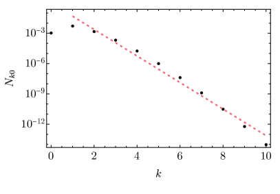
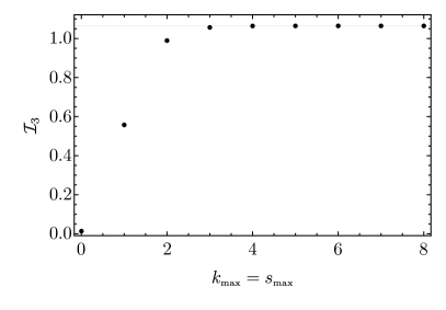
Figure 2: Left panel: Coefficients $N_{ks}$ as a function of k, fixing $s=0$. The red dashed line report a scaling $N_{k0}\propto 1/(k_{*}r_{m})^{3k}$. Right panel: Values of ${\cal I}_{3}$ as a function of the maximum index included in the sum (6.5).

Correction to the density variance. The effect of the renormalization of the composite operator can be quantified as follows. We first consider its impact on the variance of the field. With a narrow power spectrum, the Gaussian component of the curvature perturbation is characterised by a mean peak profile $\zeta_{g}(r)=\zeta_{\rm pk}\sin(k_{*}r)/(k_{*}r)$. We fix the amplitude of the curvature perturbation in such a way that it corresponds to a realisation of density contrast with the expectation value $\delta_{l}\approx\sigma_{\delta(r_{m})}$. We find

$$\left[\delta^{2}(r_{m},\vec{x}_{\rm pk})\right]=0.022+0.015\left(\frac{f_{NL}}{5/2}\right)+0.019\left(\frac{f_{NL}}{5/2}\right)^{2}-0.0016\left(\frac{g_{NL}}{25/6}\right),$$ (6.16)

which should be compared with the bare quantity $\delta^{2}(r_{m})\approx\sigma_{\delta(r_{m})}^{2}=0.022$. This propagates on the smoothed density contrast, which can be estimated as

$$\delta_{m}(r_{m},\vec{x}_{\rm pk})=0.14+0.00091\left(\frac{f_{NL}}{5/2}\right)-0.0070\left(\frac{f_{NL}}{5/2}\right)^{2}+0.00075\left(\frac{g_{NL}}{25/6}\right).$$ (6.17)

Correction to the threshold. In order to evaluate the correction to the PBH threshold for collapse, one should estimate the renormalization of the composite operators assuming the fields amplitude reach the threshold $\delta_{c}$. We fix the amplitude of the Gaussian curvature perturbation $\zeta_{g}$ assuming it leads to a collapsing overdensity with threshold amplitude $\delta_{m}=\delta_{c}$, where for a narrow spectrum we take $\delta_{c}=0.59$ [23]. This corresponds to $\delta_{l}=0.88$ and $\zeta_{\rm pk}=0.68$. In this case, we find

$$\left[\delta^{2}(r_{m},\vec{x}_{\rm pk})\right]=0.78+0.091\left(\frac{f_{NL}}{5/2}\right)+0.66\left(\frac{f_{NL}}{5/2}\right)^{2}-0.031\left(\frac{g_{NL}}{25/6}\right),$$ (6.18)

while its bare value is $\delta^{2}(r_{m})\approx 0.78$. In terms of smoothed density contrast, the renormalisation of the quadratic operators gives

$$\delta_{m}(r_{m},\vec{x}_{\rm pk})=0.59+0.20\left(\frac{f_{NL}}{5/2}\right)-0.25\left(\frac{f_{NL}}{5/2}\right)^{2}+0.020\left(\frac{g_{NL}}{25/6}\right).$$ (6.19)

7 Comments and conclusions

We have shown that in the renormalization of the quadratic power of the smoothed density contrast, a composite operator entering in the calculation of the PBH abundance, leads to the well-known phenomenon of operator mixing due to the non-Gaussian nature of the curvature perturbation. The mixing gives to an infinite tower of operators due to the necessary operation of smoothing out with the top-hat window function in real space. There are some comments we can offer at this stage:

1. The calculation of the PBH abundance is not as straightforward as standardly assumed. Not only non-linear corrections entering in the calculation of the PBH from the non-linear radiation transfer function and the determination of the true physical horizon crossing are important and lead to large uncertainties in the final result [27], but also the renormalization procedure leads to an infinite tower of operators, making the calculation of the formation probability of the PBH a difficult task. Our findings indicate a large impact on the threshold for PBH formation, depending on the sign of the non-Gaussianity parameters. Since in ultra-slow inflation the sign of the parameter $f_{NL}$ is always positive [61], our results indicate that the threshold might in fact decrease due to quadratic corrections ${\cal O}(f_{NL}^{2})$, thus increasing the PBH abundance and reversing the ${\cal O}(f_{NL})$ impact.

2. The one-loop operator mixing leads to an infinite tower of operators, made of quadratic powers of the density contrast $\delta$ and higher-derivatives thereof. Furthermore, the mixing occurs as well with non-local operators if considered from the point of view of the smoothed density contrast (or local if expressed in terms of the original curvature perturbation). Maybe one can intuitively understand why an infinite tower of operators is needed by the following argument. Around the peak of the curvature perturbation, one can perform a rotation of the coordinate axes to be aligned with the principal axes of length $\lambda_{i}$ ($i=1,2,3$) of the constant-curvature perturbation ellipsoid and Taylor expanding up to second-order gives [62]

   $$\zeta(r)\simeq\zeta_{\rm pk}-\frac{1}{2}\sum_{i=1}^{3}\lambda_{i}\left(x_{i}-x_{i}^{\rm pk}\right)^{2},$$ (7.1)

   and

   $$\delta(r_{m},\vec{x}_{\rm pk})=-\frac{4}{3}r_{m}\zeta^{\prime}(r_{m})\simeq\frac{8}{3}\left[\zeta_{\rm pk}-\zeta(r_{m})\right].$$ (7.2)

   This shows that already at the linear level, the statistics of the smoothed density contrast calculated in a volume of radius $r_{m}$ demands knowing all correlations of the curvature perturbation in two different spatial points [34] and therefore all its gradients.

3. In an idealized scenario, one might envisage to calculate the PBH abundance by involving only superhorizon physics to avoid the complications arising at horizon crossing, and thus relying on the fact that the comoving number of peaks which eventually will collapse into PBHs at horizon crossing remains constant on superhorizon scales. The renormalization procedure however must be applied as well on superhorizon scales as composite operators probe short scales and the latter may combine in the loops to generate long modes. Therefore, even on superhorizon scales calculating the PBH formation probability might be more involved than naively thought.

4. The probability of forming a PBH should not depend on any smoothing procedure, and therefore should be independent of any window function we decide to force into the calculation of the PBH abundance. The renormalization procedure is exactly performed to leave no sign of such arbitrary choice. Being the non-linear density contrast $\delta_{\rm com}(\vec{x},t)$ on comoving orthogonal slicings (2.2) a composite operator in terms of the time independent curvature perturbation $\zeta(\vec{x})$, one concludes that its renormalization should be performed in order to lead to a result independent of the choice of the smoothing procedure.

We intend to elaborate about these points in future work.

Acknowledgments.

We thank V. De Luca for useful discussions. A.I. and A.R. acknowledge support from the Swiss National Science Foundation (project number CRSII5_213497). D. P. and A.R. are supported by the Boninchi Foundation for the project “PBHs in the Era of GW Astronomy”.

Appendix A Integrals involving the Gegenbauer polynomials

A.1 Integral of one window function

The window function $W_{3}(|\vec{k}-\vec{q}|r_{m})$, defined as

$$W_{3}(x)=2^{3/2}\Gamma(5/2)\frac{J_{3/2}(x)}{x^{3/2}},$$ (A.1)

can be treated in the following way. First we use the property

$$\frac{J_{\nu}(|\vec{l}_{1}+\vec{l}_{2}|)}{|\vec{l}_{1}+\vec{l}_{2}|^{\nu}}=2^{\nu}\Gamma(\nu)\sum_{k=0}^{\infty}(\nu+k)\frac{J_{\nu+k}(l_{1})}{l_{1}^{\nu}}\frac{J_{\nu+k}(l_{2})}{l_{2}^{\nu}}C_{k}^{\nu}(\cos\theta),$$ (A.2)

where $C_{k}^{\nu}(\cos\theta)$ are the Gegenbauer polynomials and $\theta$ is the angle between the vectors $\vec{l}_{1}$ and $\vec{l}_{2}$. In general

$$\int_{0}^{\pi}{\rm d}\theta\,C^{\nu}_{k}(\cos\theta)\sin^{2\nu}\theta=0,\quad\forall\;k\neq 0.$$ (A.3)

Therefore,

$$\int\frac{{\rm d}\Omega}{4\pi}\frac{J_{1/2}(|\vec{l}_{1}+\vec{l}_{2}|)}{|\vec{l}_{1}+\vec{l}_{2}|^{1/2}} = 2^{1/2}\Gamma(1/2)\frac{1}{2}\frac{J_{1/2}(l_{1})}{l_{1}^{1/2}}\frac{J_{1/2}(l_{2})}{l_{2}^{1/2}}\int\frac{{\rm d}\Omega}{4\pi}C_{0}^{1/2}(\cos\theta)\;+$$ (A.4)

$$+ 2^{1/2}\Gamma(1/2)\sum_{k=1}^{\infty}(1/2+k)\frac{J_{1/2+k}(l_{1})}{l_{1}^{1/2}}\frac{J_{1/2+k}(l_{2})}{l_{2}^{1/2}}\int\frac{{\rm d}\Omega}{4\pi}C_{k}^{1/2}(\cos\theta).$$

Only the first term in the sum is not zero, leading to the simple relation

$$\int\frac{{\rm d}\Omega}{4\pi}\frac{J_{1/2}(|\vec{l}_{1}+\vec{l}_{2}|)}{|\vec{l}_{1}+\vec{l}_{2}|^{1/2}}=2^{1/2}\Gamma(1/2)\frac{1}{2}\frac{J_{1/2}(l_{1})}{l_{1}^{1/2}}\frac{J_{1/2}(l_{2})}{l_{2}^{1/2}}.$$ (A.5)

Now we can use the general relations

$$l\frac{{\rm d}}{{\rm d}l}\frac{J_{D/2-1}(l)}{l^{D/2-1}}=-\frac{J_{D/2}(l)}{l^{D/2-2}},$$ (A.6)

$$\frac{J_{D/2-1}(l)}{l^{D/2-1}}=l\frac{{\rm d}}{{\rm d}l}\frac{J_{D/2}(l)}{l^{D/2}}+D\frac{J_{D/2}(l)}{l^{D/2}},$$ (A.7)

to transform the equation above from $J_{1/2}$ to $J_{3/2}$, using the relation

$$l_{1}\partial_{l_{1}}\frac{J_{1/2}(|\vec{l}_{1}+\vec{l}_{2}|)}{|\vec{l}_{1}+\vec{l}_{2}|^{1/2}}=-(l_{1}^{2}+\vec{l}_{1}\cdot\vec{l}_{2})\frac{J_{3/2}(|\vec{l}_{1}+\vec{l}_{2}|)}{|\vec{l}_{1}+\vec{l}_{2}|^{3/2}}.$$ (A.8)

We take the derivative with respect to $l_{1}$ of Eq. (A.5), leading to

$$\int\frac{{\rm d}\Omega}{4\pi}W_{3}(|\vec{l}_{1}-\vec{l}_{2}|)\left(1-\frac{\vec{l}_{1}\cdot\vec{l}_{2}}{l_{1}^{2}}\right)=W_{3}(l_{1})W_{3}(l_{2})+W_{3}(l_{1})\;\frac{l_{2}}{3}\frac{{\rm d}}{{\rm d}l_{2}}W_{3}(l_{2}).$$ (A.9)

Multiplying both sides with $l_{1}^{2}$ and summing the same relation exchanging $l_{1}$ with $l_{2}$, we get

$$\int\frac{{\rm d}\Omega}{4\pi}W_{3}(|\vec{l}_{1}-\vec{l}_{2}|)\left(l_{1}^{2}+l_{2}^{2}-2\vec{l}_{1}\cdot\vec{l}_{2}\right)=\int\frac{{\rm d}\Omega}{4\pi}W_{3}(|\vec{l}_{1}-\vec{l}_{2}|)|\vec{l}_{1}-\vec{l}_{2}|^{2}=$$

$$=W_{3}(l_{1})W_{3}(l_{2})(l_{1}^{2}+l_{2}^{2})+W_{3}(l_{1})\;\frac{l_{1}^{2}l_{2}}{3}\frac{{\rm d}}{{\rm d}l_{2}}W_{3}(l_{2})+W_{3}(l_{2})\;\frac{l_{2}^{2}l_{1}}{3}\frac{{\rm d}}{{\rm d}l_{1}}W_{3}(l_{1})=$$

$$=W_{3}(l_{1})W_{3}(l_{2})\left(l_{1}^{2}+l_{2}^{2}+\frac{l_{1}^{2}l_{2}}{3W_{3}(l_{2})}\frac{{\rm d}}{{\rm d}l_{2}}W_{3}(l_{2})+\;\frac{l_{2}^{2}l_{1}}{3W_{3}(l_{1})}\frac{{\rm d}}{{\rm d}l_{1}}W_{3}(l_{1})\right).$$ (A.10)

A.2 Integral with two window functions

For the composite operator with two external legs, we have to evaluate the following momentum integral

$$I =\int_{\vec{l}_{1}}|\vec{l}_{1}+\vec{l}_{2}|^{2}W_{3}(|\vec{l}_{1}+\vec{l}_{2}|)|\vec{l}_{1}+\vec{l}_{3}|^{2}W_{3}(|\vec{l}_{1}+\vec{l}_{3}|)$$

$$=\int_{\vec{l}_{1}}(l_{1}^{2}+l_{2}^{2}+2l_{1}l_{2}\cos\theta_{12})W_{3}(|\vec{l}_{1}+\vec{l}_{2}|)(l_{1}^{2}+l_{3}^{2}+2l_{1}l_{3}\cos\theta_{13})W_{3}(|\vec{l}_{1}+\vec{l}_{3}|)$$

$$=\int_{\vec{l}_{1}}\Big{(}A_{00}+A_{10}\cos\theta_{12}+A_{01}\cos\theta_{13}+A_{11}\cos\theta_{12}\cos\theta_{13}\Big{)}W_{3}(|\vec{l}_{1}+\vec{l}_{2}|)W_{3}(|\vec{l}_{1}+\vec{l}_{3}|)$$

$$=2^{3}\Gamma^{2}(5/2)\int_{\vec{l}_{1}}\Big{(}A_{00}+A_{10}\cos\theta_{12}+A_{01}\cos\theta_{13}+A_{11}\cos\theta_{12}\cos\theta_{13}\Big{)}\frac{J_{3/2}(|\vec{l}_{1}+\vec{l}_{2}|)}{|\vec{l}_{1}+\vec{l}_{2}|^{3/2}}\frac{J_{3/2}(|\vec{l}_{1}+\vec{l}_{3}|)}{|\vec{l}_{1}+\vec{l}_{3}|^{3/2}},$$ (A.11)

where

$$A_{00}=l_{1}^{4}+l_{1}^{2}(l_{2}^{2}+l_{3}^{2})+l_{2}^{2}l_{3}^{2},~{}~{}~{}~{}~{}A_{10}=2l_{1}l_{2}(l_{1}^{2}+l_{3}^{2}),$$

$$A_{01}=2l_{1}l_{3}(l_{1}^{2}+l_{2}^{2}),~{}~{}~{}~{}~{}~{}~{}~{}~{}~{}~{}~{}~{}~{}~{}~{}~{}A_{11}=4l_{1}^{2}l_{2}l_{3}.$$ (A.12)

We have parametrized the vectors $\vec{l_{i}}$ as

$$\vec{l}_{2}=l_{2}\;(0,\;0,\;1),$$

$$\vec{l}_{3}=l_{3}\;(0,\;\sqrt{1-y^{2}},\;y),$$

$$\vec{l}_{1}=l_{1}\;(\cos\beta\sqrt{1-x^{2}},\;\sin\beta\sqrt{1-x^{2}},\;x),$$ (A.13)

so that

$$\cos\theta_{12}=x,~{}~{}~{}~{}~{}\cos\theta_{13}=xy+\sqrt{1-y^{2}}\sqrt{1-x^{2}}\sin\beta.$$ (A.14)

Using the addition theorem

$$\frac{J_{\nu}(|\vec{l}_{1}+\vec{l}_{2}|)}{|\vec{l}_{1}+\vec{l}_{2}|^{\nu}}\frac{J_{\nu}(|\vec{l}_{1}+\vec{l}_{3}|)}{|\vec{l}_{1}+\vec{l}_{3}|^{\nu}} =(2^{\nu}\Gamma(\nu))^{2}\sum_{k=0}^{\infty}\sum_{s=0}^{\infty}\frac{J_{\nu+k}(l_{1})}{l_{1}^{\nu}}\frac{J_{\nu+k}(l_{2})}{l_{2}^{\nu}}\frac{J_{\nu+s}(l_{1})}{l_{1}^{\nu}}\frac{J_{\nu+s}(l_{3})}{l_{3}^{\nu}}$$

$$\cdot(\nu+k)(\nu+s)C_{k}^{\nu}(\cos\theta_{12})C_{s}^{\nu}(\cos\theta_{13}),$$ (A.15)

we can express the integral (A.11) as

$$I =\int_{\vec{l}_{1}}\Big{(}A_{00}+A_{10}\cos\theta_{12}+A_{01}\cos\theta_{13}+A_{11}\cos\theta_{12}\cos\theta_{13}\Big{)}\sum_{k=0}^{\infty}\sum_{s=0}^{\infty}9\pi^{2}\left(\frac{3}{2}+k\right)$$

$$\cdot\left(\frac{3}{2}+s\right)\frac{J_{3/2+k}(l_{1})}{l_{1}^{3/2}}\frac{J_{3/2+k}(l_{2})}{l_{2}^{3/2}}\frac{J_{3/2+s}(l_{1})}{l_{1}^{3/2}}\frac{J_{3/2+s}(l_{3})}{l_{3}^{3/2}}C_{k}^{3/2}(\cos\theta_{12})C_{s}^{3/2}(\cos\theta_{13}).$$ (A.16)

Therefore, the integral (A.11) can be written as

$$I=\sum_{i,j=0}^{1}\int\frac{l^{2}{\rm d}l}{2\pi^{2}}A_{ij}I^{ij},$$ (A.17)

where

$$I^{ij}=\sum_{k=0}^{\infty}\sum_{s=0}^{\infty}N_{ks}I^{ij}_{ks}(y),$$ (A.18)

$$N_{ks} =9\pi^{2}\left(\frac{3}{2}+k\right)\left(\frac{3}{2}+s\right)\frac{J_{3/2+k}(l_{1})}{l_{1}^{3/2}}\frac{J_{3/2+k}(l_{2})}{l_{2}^{3/2}}\frac{J_{3/2+s}(l_{1})}{l_{1}^{3/2}}\frac{J_{3/2+s}(l_{3})}{l_{3}^{3/2}}$$

$$=\frac{4}{9}\left(\frac{3}{2}+k\right)\left(\frac{3}{2}+s\right)\left[l_{1}^{k}\left(\frac{1}{l_{1}}\frac{{\rm d}}{{\rm d}l_{1}}\right)^{k}W_{3}(l_{1})\right]\left[l_{1}^{s}\left(\frac{1}{l_{1}}\frac{{\rm d}}{{\rm d}l_{1}}\right)^{s}W_{3}(l_{1})\right]$$

$$~{}~{}\times\left[l_{2}^{k}\left(\frac{1}{l_{2}}\frac{{\rm d}}{{\rm d}l_{2}}\right)^{k}W_{3}(l_{2})\right]\left[l_{3}^{s}\left(\frac{1}{l_{3}}\frac{{\rm d}}{{\rm d}l_{3}}\right)^{s}W_{3}(l_{3})\right],$$ (A.19)

and

$$I^{ij}_{ks}(y=\cos\theta_{23})=\int\frac{{\rm d}\Omega}{4\pi}(\cos\theta_{12})^{i}(\cos\theta_{13})^{j}C_{k}^{3/2}(\cos\theta_{12})C_{s}^{3/2}(\cos\theta_{13}).$$ (A.20)

Therefore, in order to calculate Eq. (A.11), we need to calculate the four integrals

$$I^{00}_{ks}(y),~{}I^{10}_{ks}(y),~{}I^{01}_{ks}(y),~{}~{}~{}\mbox{and}~{}~{}~{}I^{11}_{ks}(y),$$ (A.21)

which we will do in the following. Inserting the angles (A.14) and using the fact that

$$\int_{0}^{2\pi}\frac{{\rm d}\beta}{2\pi}\,C_{k}^{3/2}\left(xy+\sqrt{1-y^{2}}\sqrt{1-x^{2}}\sin\beta\right) =\left\{\begin{array}[]{lll}{\displaystyle{\sum_{n={\rm even}}^{k}}}(2n+1)P_{n}(x)P_{n}(y)&~{}{\rm if}&~{}k=\mbox{even},\\ &&\\ {\displaystyle{\sum_{n={\rm odd}}^{k}}}(2n+1)P_{n}(x)P_{n}(y)&~{}{\rm if}&~{}k=\mbox{odd},\\ \end{array}\right.$$ (A.25)

and

$$C_{k}^{3/2}(x) =\frac{{\rm d}}{{\rm d}x}P_{k+1}(x)$$

$$=(2k+1)P_{k}(x)+\Big{(}2(k-2)+1\Big{)}P_{k-2}(x)+\Big{(}2(k-4)+1\Big{)}P_{k-4}(x)+\cdots,$$ (A.26)

the integration over the angles gives

$$I^{00}_{ks} =\int\frac{{\rm d}\Omega}{4\pi}C_{k}^{3/2}(x)C_{s}^{3/2}\left(xy+\sqrt{1-y^{2}}\sqrt{1-x^{2}}\sin\beta\right)=$$

$$\hskip 113.81102pt=\left\{\begin{array}[]{lll}\dfrac{{\rm d}}{{\rm d}y}P_{{\rm min}(k,s)+1}(y)&{\rm if}&(k,s)\in 2{\mathbb{N}},\\ &&\\ \dfrac{{\rm d}}{{\rm d}y}P_{{\rm min}(k,s)+1}(y)&{\rm if}&(k,s)\in 2{\mathbb{N}}+1,\\ &&\\ 0&{\rm otherwise},&\\ \end{array}\right.,$$ (A.32)

or

$$I^{00}_{ks}=\left(\frac{1+(-1)^{k+s}}{2}\right)\dfrac{{\rm d}}{{\rm d}y}P_{{\rm min}(k,s)+1}(y).$$ (A.33)

The next integral to evaluate is

$$I_{ks}^{10}(y)=\int\frac{{\rm d}\Omega}{4\pi}\,x\,C_{k}^{3/2}(x)C_{s}^{3/2}(\cos\theta_{13}).$$ (A.34)

To proceed, we need the recursive relation of Legendre polynomials

$$x\frac{{\rm d}P_{k+1}(x)}{{\rm d}x}=\frac{{\rm d}P_{k+2}(x)}{{\rm d}x}-(k+2)P_{k+1}(x),$$ (A.35)

which can be written as

$$x\,C_{k}^{3/2}(x)=C^{3/2}_{k+1}-(k+2)P_{k+1}(x).$$ (A.36)

Then, using Eq. (A.25), we can easily see that

$$\int_{0}^{2\pi}\frac{{\rm d}\Omega}{4\pi}\,P_{k+1}(x)C_{s}^{3/2}(\cos\theta_{13})=\left\{\begin{array}[]{lll}\Theta(s-k-1)\,P_{k+1}(y)&{\rm if}&(k,s)\in 2{\mathbb{N}},\\ &&\\ \Theta(s-k-1)\,P_{k+1}(y)&{\rm if}&(k,s)\in 2{\mathbb{N}}+1,\\ &&\\ 0&{\rm otherwise},&\\ \end{array}\right.$$ (A.42)

where $\Theta(n)=0$ for $n<0$ and $\Theta(n)=1$ for $n\geq 0$. Therefore, using Eqs. (A.36) and (A.42), we find that

$$I^{10}_{ks}=\left(\frac{1-(-1)^{k+s}}{2}\right)\left[\Theta(k-s)\frac{\rm d}{{\rm d}y}P_{k+1}(y)+\Theta(s-k)y\frac{\rm d}{{\rm d}y}P_{s+1}(y)\right]$$ (A.43)

To calculate $I^{01}$ we need the relation

$$\int_{0}^{2\pi}\frac{{\rm d}\beta}{2\pi}\, \cos\theta_{13}C_{k}^{3/2}\left(\cos\theta_{13}\right)=$$

$$=\left\{\begin{array}[]{lll}2(k+1)P_{k+1}(x)P_{k+1}(y)+{\displaystyle{\sum_{n={\rm odd}}^{k}}}2(2n+1)P_{n}(x)P_{n}(y)&~{}{\rm if}&~{}k=\mbox{even},\\ &&\\ 2(k+1)P_{k+1}(x)P_{k+1}(y)+{\displaystyle{\sum_{n={\rm even}}^{k}}}2(2n+1)P_{n}(x)P_{n}(y)&~{}{\rm if}&~{}k=\mbox{odd},\\ \end{array}\right.$$ (A.47)

Then, by using Eq. (A.26), we find that the integral

$$I^{01}_{ks} = \int\frac{{\rm d}\Omega}{4\pi}\,C^{3/2}_{k}(x)\cos\theta_{13}C_{s}^{3/2}(\cos\theta_{13})$$ (A.48)

turns out to be

$$I^{01}_{ks}=\left(\frac{1-(-1)^{k+s}}{2}\right)\left[\Theta(s-k)\frac{\rm d}{{\rm d}y}P_{k+1}(y)+\Theta(k-s)y\frac{\rm d}{{\rm d}y}P_{s+1}(y)\right].$$ (A.49)

The final integral $I^{11}_{ks}$ can be calculated using Eq. (A.36). The result is

$$I^{11}_{ks}=I^{01}_{k+1,s}-(k+2)\left\{\left(\frac{1+(-1)^{k+s}}{2}\right)\Theta(s-k-1)P_{k+1}(y)+\frac{s+1}{2s+3}\delta_{sk}P_{s+1}(y)\right\}.$$ (A.50)

Appendix B Non-local operators

To derive the expression (5.12), we start Eq. (4.3) which can be rewritten as

$$\frac{\delta(r_{m},\vec{x}_{\rm pk})}{r_{m}^{2}}=\frac{4}{9}\nabla^{2}_{x_{\rm pk}}\int_{\vec{k}}\;e^{i\vec{k}\cdot\vec{x}_{\rm pk}}W_{3}(kr_{m})\zeta_{\vec{k}}.$$ (B.1)

We now take the derivative $r_{m}\partial_{r_{m}}$ of both sides to get

$$\frac{1}{r_{m}}\partial_{r}\delta(r,\vec{x}_{\rm pk})\Big{|}_{r=r_{m}}=-2\frac{\delta(r_{m},\vec{x}_{\rm pk})}{r_{m}^{2}}+\frac{1}{r_{m}}\partial_{r}\delta(r,\vec{x}_{\rm pk})\Big{|}_{r=r_{m}}=\frac{4}{9}\nabla^{2}_{x_{\rm pk}}\int_{\vec{k}}\;e^{i\vec{k}\cdot\vec{x}_{\rm pk}}\zeta_{\vec{k}}\,r_{m}\partial_{r}W_{3}(kr)\Big{|}_{r=r_{m}}.$$ (B.2)

By using Eq. (2.4) we get

$$\partial_{r}\delta(r,\vec{x}_{\rm pk})\Big{|}_{r=r_{m}}=0,$$ (B.3)

and consequently

$$-2\frac{\delta(r_{m},\vec{x}_{\rm pk})}{r_{m}^{2}}=\frac{4}{9}\nabla^{2}_{x_{\rm pk}}\int_{\vec{k}}\;e^{i\vec{k}\cdot\vec{x}_{\rm pk}}\zeta_{\vec{k}}\,r_{m}\partial_{r}W_{3}(kr)\Big{|}_{r=r_{m}}$$ (B.4)

or

$$r_{m}\partial_{r}W_{3}(kr)\Big{|}_{r=r_{m}}\zeta_{\vec{k}}=-\frac{9}{2r_{m}^{2}}\int_{\vec{x}_{\rm pk}}\;e^{-i\vec{k}\cdot\vec{x}_{\rm pk}}\;\nabla^{-2}_{x_{\rm pk}}\delta(r_{m},\vec{x}_{\rm pk})$$ (B.5)

which is a non-local operator.

References

- [1] M. Sasaki, T. Suyama, T. Tanaka and S. Yokoyama, Primordial black holes—perspectives in gravitational wave astronomy, Class. Quant. Grav. 35 (2018) 063001, [1801.05235].
- [2] B. Carr, K. Kohri, Y. Sendouda and J. Yokoyama, Constraints on primordial black holes, Rept. Prog. Phys. 84 (2021) 116902, [2002.12778].
- [3] A. M. Green and B. J. Kavanagh, Primordial Black Holes as a dark matter candidate, J. Phys. G 48 (2021) 043001, [2007.10722].
- [4] LISA Cosmology Working Group collaboration, E. Bagui et al., Primordial black holes and their gravitational-wave signatures, 2310.19857.
- [5] LIGO Scientific, Virgo collaboration, B. P. Abbott et al., Observation of Gravitational Waves from a Binary Black Hole Merger, Phys. Rev. Lett. 116 (2016) 061102, [1602.03837].
- [6] LIGO Scientific, Virgo collaboration, B. P. Abbott et al., GWTC-1: A Gravitational-Wave Transient Catalog of Compact Binary Mergers Observed by LIGO and Virgo during the First and Second Observing Runs, Phys. Rev. X 9 (2019) 031040, [1811.12907].
- [7] LIGO Scientific, Virgo collaboration, R. Abbott et al., GWTC-2: Compact Binary Coalescences Observed by LIGO and Virgo During the First Half of the Third Observing Run, Phys. Rev. X 11 (2021) 021053, [2010.14527].
- [8] LIGO Scientific, VIRGO, KAGRA collaboration, R. Abbott et al., GWTC-3: Compact Binary Coalescences Observed by LIGO and Virgo During the Second Part of the Third Observing Run, 2111.03606.
- [9] S. Bird, I. Cholis, J. B. Muñoz, Y. Ali-Haïmoud, M. Kamionkowski, E. D. Kovetz et al., Did LIGO detect dark matter?, Phys. Rev. Lett. 116 (2016) 201301, [1603.00464].
- [10] M. Sasaki, T. Suyama, T. Tanaka and S. Yokoyama, Primordial Black Hole Scenario for the Gravitational-Wave Event GW150914, Phys. Rev. Lett. 117 (2016) 061101, [1603.08338].
- [11] S. Clesse and J. García-Bellido, The clustering of massive Primordial Black Holes as Dark Matter: measuring their mass distribution with Advanced LIGO, Phys. Dark Univ. 15 (2017) 142–147, [1603.05234].
- [12] Y. Ali-Haïmoud, E. D. Kovetz and M. Kamionkowski, Merger rate of primordial black-hole binaries, Phys. Rev. D 96 (2017) 123523, [1709.06576].
- [13] G. Hütsi, M. Raidal, V. Vaskonen and H. Veermäe, Two populations of LIGO-Virgo black holes, JCAP 03 (2021) 068, [2012.02786].
- [14] V. De Luca, G. Franciolini, P. Pani and A. Riotto, Bayesian Evidence for Both Astrophysical and Primordial Black Holes: Mapping the GWTC-2 Catalog to Third-Generation Detectors, JCAP 05 (2021) 003, [2102.03809].
- [15] G. Franciolini, V. Baibhav, V. De Luca, K. K. Y. Ng, K. W. K. Wong, E. Berti et al., Searching for a subpopulation of primordial black holes in LIGO-Virgo gravitational-wave data, Phys. Rev. D 105 (2022) 083526, [2105.03349].
- [16] G. Franciolini, I. Musco, P. Pani and A. Urbano, From inflation to black hole mergers and back again: Gravitational-wave data-driven constraints on inflationary scenarios with a first-principle model of primordial black holes across the QCD epoch, Phys. Rev. D 106 (2022) 123526, [2209.05959].
- [17] Z.-C. Chen and Q.-G. Huang, Distinguishing Primordial Black Holes from Astrophysical Black Holes by Einstein Telescope and Cosmic Explorer, JCAP 08 (2020) 039, [1904.02396].
- [18] O. Pujolas, V. Vaskonen and H. Veermäe, Prospects for probing gravitational waves from primordial black hole binaries, Phys. Rev. D 104 (2021) 083521, [2107.03379].
- [19] V. De Luca, G. Franciolini, P. Pani and A. Riotto, The minimum testable abundance of primordial black holes at future gravitational-wave detectors, JCAP 11 (2021) 039, [2106.13769].
- [20] S. Barsanti, V. De Luca, A. Maselli and P. Pani, Detecting Subsolar-Mass Primordial Black Holes in Extreme Mass-Ratio Inspirals with LISA and Einstein Telescope, Phys. Rev. Lett. 128 (2022) 111104, [2109.02170].
- [21] S. S. Bavera, G. Franciolini, G. Cusin, A. Riotto, M. Zevin and T. Fragos, Stochastic gravitational-wave background as a tool for investigating multi-channel astrophysical and primordial black-hole mergers, Astron. Astrophys. 660 (2022) A26, [2109.05836].
- [22] I. Musco, Threshold for primordial black holes: Dependence on the shape of the cosmological perturbations, Phys. Rev. D 100 (2019) 123524, [1809.02127].
- [23] I. Musco, V. De Luca, G. Franciolini and A. Riotto, Threshold for primordial black holes. II. A simple analytic prescription, Phys. Rev. D 103 (2021) 063538, [2011.03014].
- [24] V. De Luca, G. Franciolini, A. Kehagias, M. Peloso, A. Riotto and C. Ünal, The Ineludible non-Gaussianity of the Primordial Black Hole Abundance, JCAP 07 (2019) 048, [1904.00970].
- [25] S. Young, I. Musco and C. T. Byrnes, Primordial black hole formation and abundance: contribution from the non-linear relation between the density and curvature perturbation, JCAP 11 (2019) 012, [1904.00984].
- [26] S. Young, The primordial black hole formation criterion re-examined: Parametrisation, timing and the choice of window function, Int. J. Mod. Phys. D 29 (2019) 2030002, [1905.01230].
- [27] V. De Luca, A. Kehagias and A. Riotto, How well do we know the primordial black hole abundance: The crucial role of nonlinearities when approaching the horizon, Phys. Rev. D 108 (2023) 063531, [2307.13633].
- [28] G. Ferrante, G. Franciolini, A. Iovino, Junior. and A. Urbano, Primordial non-Gaussianity up to all orders: Theoretical aspects and implications for primordial black hole models, Phys. Rev. D 107 (2023) 043520, [2211.01728].
- [29] M. Biagetti, V. De Luca, G. Franciolini, A. Kehagias and A. Riotto, The formation probability of primordial black holes, Phys. Lett. B 820 (2021) 136602, [2105.07810].
- [30] M. Shibata and M. Sasaki, Black hole formation in the Friedmann universe: Formulation and computation in numerical relativity, Phys. Rev. D 60 (1999) 084002, [gr-qc/9905064].
- [31] T. Harada, C.-M. Yoo, T. Nakama and Y. Koga, Cosmological long-wavelength solutions and primordial black hole formation, Phys. Rev. D 91 (2015) 084057, [1503.03934].
- [32] A. Escrivà, C. Germani and R. K. Sheth, Universal threshold for primordial black hole formation, Phys. Rev. D 101 (2020) 044022, [1907.13311].
- [33] C. Germani and R. K. Sheth, Nonlinear statistics of primordial black holes from Gaussian curvature perturbations, Phys. Rev. D 101 (2020) 063520, [1912.07072].
- [34] V. De Luca and A. Riotto, A note on the abundance of primordial black holes: Use and misuse of the metric curvature perturbation, Phys. Lett. B 828 (2022) 137035, [2201.09008].
- [35] A. D. Gow, H. Assadullahi, J. H. P. Jackson, K. Koyama, V. Vennin and D. Wands, Non-perturbative non-Gaussianity and primordial black holes, EPL 142 (2023) 49001, [2211.08348].
- [36] N. Bartolo, E. Komatsu, S. Matarrese and A. Riotto, Non-Gaussianity from inflation: Theory and observations, Phys. Rept. 402 (2004) 103–266, [astro-ph/0406398].
- [37] Planck collaboration, Y. Akrami et al., Planck 2018 results. IX. Constraints on primordial non-Gaussianity, Astron. Astrophys. 641 (2020) A9, [1905.05697].
- [38] Y.-F. Cai, X. Chen, M. H. Namjoo, M. Sasaki, D.-G. Wang and Z. Wang, Revisiting non-Gaussianity from non-attractor inflation models, JCAP 05 (2018) 012, [1712.09998].
- [39] N. Bartolo, S. Matarrese and A. Riotto, On nonGaussianity in the curvaton scenario, Phys. Rev. D 69 (2004) 043503, [hep-ph/0309033].
- [40] M. Sasaki, J. Valiviita and D. Wands, Non-Gaussianity of the primordial perturbation in the curvaton model, Phys. Rev. D 74 (2006) 103003, [astro-ph/0607627].
- [41] NANOGrav collaboration, G. Agazie et al., The NANOGrav 15 yr Data Set: Evidence for a Gravitational-wave Background, Astrophys. J. Lett. 951 (2023) L8, [2306.16213].
- [42] NANOGrav collaboration, G. Agazie et al., The NANOGrav 15 yr Data Set: Observations and Timing of 68 Millisecond Pulsars, Astrophys. J. Lett. 951 (2023) L9, [2306.16217].
- [43] EPTA collaboration, J. Antoniadis et al., The second data release from the european pulsar timing array iii. search for gravitational wave signals, 2306.16214.
- [44] EPTA collaboration, J. Antoniadis et al., The second data release from the european pulsar timing array i. the dataset and timing analysis, 2306.16224.
- [45] EPTA collaboration, J. Antoniadis et al., The second data release from the european pulsar timing array: V. implications for massive black holes, dark matter and the early universe, 2306.16227.
- [46] D. J. Reardon et al., Search for an Isotropic Gravitational-wave Background with the Parkes Pulsar Timing Array, Astrophys. J. Lett. 951 (2023) L6, [2306.16215].
- [47] PPTA collaboration, A. Zic et al., The parkes pulsar timing array third data release, 2306.16230.
- [48] D. J. Reardon et al., The Gravitational-wave Background Null Hypothesis: Characterizing Noise in Millisecond Pulsar Arrival Times with the Parkes Pulsar Timing Array, Astrophys. J. Lett. 951 (2023) L7, [2306.16229].
- [49] H. Xu et al., Searching for the Nano-Hertz Stochastic Gravitational Wave Background with the Chinese Pulsar Timing Array Data Release I, Res. Astron. Astrophys. 23 (2023) 075024, [2306.16216].
- [50] G. Franciolini, A. Iovino, Junior., V. Vaskonen and H. Veermae, The recent gravitational wave observation by pulsar timing arrays and primordial black holes: the importance of non-gaussianities, 2306.17149.
- [51] L. Liu, Z.-C. Chen and Q.-G. Huang, Implications for the non-Gaussianity of curvature perturbation from pulsar timing arrays, 2307.01102.
- [52] S. Wang, Z.-C. Zhao, J.-P. Li and Q.-H. Zhu, Exploring the Implications of 2023 Pulsar Timing Array Datasets for Scalar-Induced Gravitational Waves and Primordial Black Holes, 2307.00572.
- [53] Y.-F. Cai, X.-C. He, X. Ma, S.-F. Yan and G.-W. Yuan, Limits on scalar-induced gravitational waves from the stochastic background by pulsar timing array observations, 2306.17822.
- [54] K. Inomata, K. Kohri and T. Terada, The Detected Stochastic Gravitational Waves and Sub-Solar Primordial Black Holes, 2306.17834.
- [55] D. G. Figueroa, M. Pieroni, A. Ricciardone and P. Simakachorn, Cosmological Background Interpretation of Pulsar Timing Array Data, 2307.02399.
- [56] Z. Yi, Q. Gao, Y. Gong, Y. Wang and F. Zhang, The waveform of the scalar induced gravitational waves in light of Pulsar Timing Array data, 2307.02467.
- [57] Q.-H. Zhu, Z.-C. Zhao and S. Wang, Joint implications of BBN, CMB, and PTA Datasets for Scalar-Induced Gravitational Waves of Second and Third orders, 2307.03095.
- [58] J. Ellis, M. Fairbairn, G. Franciolini, G. Hütsi, A. Iovino, M. Lewicki et al., What is the source of the PTA GW signal?, 2308.08546.
- [59] C. Germani and I. Musco, Abundance of Primordial Black Holes Depends on the Shape of the Inflationary Power Spectrum, Phys. Rev. Lett. 122 (2019) 141302, [1805.04087].
- [60] V. De Luca, G. Franciolini and A. Riotto, On the Primordial Black Hole Mass Function for Broad Spectra, Phys. Lett. B 807 (2020) 135550, [2001.04371].
- [61] H. Firouzjahi and A. Riotto, The Sign of non-Gaussianity and the Primordial Black Holes Abundance, 2309.10536.
- [62] J. M. Bardeen, J. R. Bond, N. Kaiser and A. S. Szalay, The Statistics of Peaks of Gaussian Random Fields, Astrophys. J. 304 (1986) 15–61.