Concurrent Design Optimization of Shared Powertrain Modules in a Family of Electric Vehicles

Abstract

We present a concurrent optimization framework to design shared modular powertrain components for a family of battery electric vehicles, whereby the modules’ sizes are jointly-optimized to minimize the family Total Cost of Ownership (TCO). As opposed to individually-tailoring the components, our approach can significantly reduce production costs due to the higher volumes of the same item. We instantiate a bi-level nested framework consisting of an inner convex optimization routine, which jointly optimizes the modules’ sizes and the powertrain operation for given driving cycles and modules’ multiplicities, and an outer loop comparing each configuration to identify the minimum-TCO family co-design solution with global optimality guarantees. Finally, we showcase our framework on a case study for the Tesla family in a benchmark design problem, considering the Model S, Model 3, Model X, and Model Y. Our results show that, compared to an individually tailored design, the application of our concurrent design optimization framework achieves a significant reduction of acquisition price for a minimal increase in operational costs, ultimately lowering the family TCO in the benchmark design problem by 3.5%. Moreover, in a sensitivity study on the market conditions considered, our concurrent design optimization methodology can reduce the TCO by up to 17%.

I Introduction

The wider diffusion of Battery Electric Vehicles (BEVs) is considered a key objective in the transition to more sustainable mobility [1]. As a matter of fact, BEVs are important tools in the fight against pollution in cities, lowering the environmental impact by significantly decreasing particulate matter [2] and CO₂ emissions [3]. Despite the efforts in promoting policies oriented to the purchase and use of BEVs [4], they still account for a small share of the total amount of vehicles due to a relatively higher price when compared to their conventional, fossil-fuel-powered counterparts [5]. The considerable upfront cost, combined with supply shortages affecting manufacturing [6], prevents the adoption of this technology by a larger share of the general public [3, 7]. In order to accelerate the transition to electric mobility, the Total Cost of Ownership (TCO) of BEVs must be reduced. Many companies have adopted design strategies aimed at developing remarkably efficient tailor-made designs [8]. However, these design choices imply considerable production costs, due to the highly specific components that are individually tailored to each vehicle model. Conversely, it is possible to reduce production costs by leveraging Economy-of-Scale (EoS) strategies, whereas increasing the amount of identical components produced reduces their specific production cost. However, this kind of approach requires large production volumes of the same item, involving a critical manufacturing ramp-up [9] and hindering diversification, pivotal to satisfying the wide range of customer needs. We aim to address these issues by investigating a module-based product family design approach (Fig. 1) to take full advantage of the EoS strategies, substantially lowering the vehicles’ TCO without limiting product diversification. Nevertheless, the mere identification of a feasible design of a shared module for multiple vehicles is a challenging task, which may result in excessive performance deterioration in the vehicles sharing the module [10]. For this reason, we resort to the application of numerical optimization to find the shared size and number of modules that every vehicle is equipped with (multiplicity), jointly optimized to minimize the TCO of the family instead of being individually tailored for every vehicle. Against this backdrop, this paper presents the concurrent design optimization framework shown in Fig. 2 to jointly optimize the size and multiplicity of shared battery and Electric Motor (EM) modules with the operations of a family of BEVs, minimizing the overall TCO.

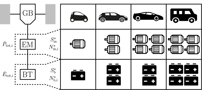
Figure 1: Family of battery electric vehicles designed leveraging a shared modular powertrain. Every vehicle type is equipped with $N_{\mathrm{m},i}^{\star}$ motor modules (EM) of size $S_{\mathrm{m}}^{\star}$ and $N_{\mathrm{b},i}^{\star}$ battery modules of size $S_{\mathrm{b}}^{\star}$, for a total maximum motor power of $\overline{P}_{\mathrm{tot},i}$ and maximum energy capacity of $\overline{E}_{\mathrm{tot},i}$.

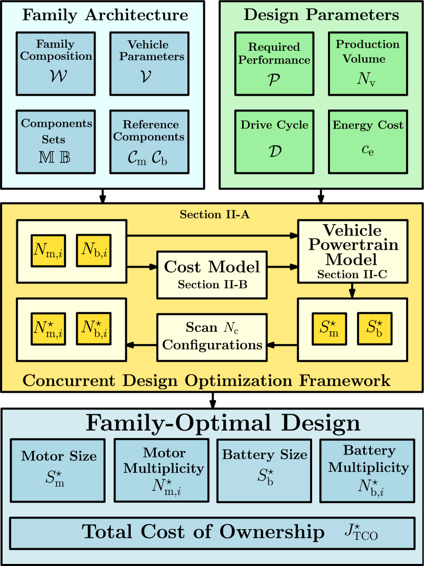
Figure 2: Concurrent design optimization methodology diagram.

Related Literature: This paper pertains to two main research lines: multi-product design and powertrain design optimization. Multi-product design is a design strategy leveraging commonality, modularity and standardization among products to reduce components’ costs, provide operational and logistical advantages in part sourcing, and quality control [11]. Moreover, it fosters the development and upgrade of differentiated products efficiently, increases flexibility and responsiveness in manufacturing processes [12], and generates substantial savings in research, testing, interface design, and integration [13]. Multi-product design consists of two main processes: platform design and product family design. The former entails the development of a product platform (consisting of a common product architecture, shared physical components and processes) from the company objectives and market research. The latter accounts for the design of products starting from the common platform. Industrial players have widely studied and employed these methodologies for different products to provide cost-effective variety and customization [14]: from the Sony Walkman [15, 16] to aircraft [17, 18] and spacecraft [19]. The automotive sector was perhaps one of the fields where multi-product design achieved the best results. Industrial giants like Volkswagen [20, 21] saved billions of dollars per year producing some of the most successful automotive platforms. In fact, “in the 1990s, automotive manufacturers that employed a platform-based product development approach gained a 5.1% market share per year while those that did not, lost 2.2%” [22]. However, the application of these strategies to electric vehicles has been delayed due to the smaller production volumes compared to conventional vehicles [1], the lack of standardization [23], and the challenges in design due to the unripened technology.

The second research stream concerns powertrain design optimization. This discipline has been thoroughly studied over the years, producing a considerable number of methods and applications [24]. In the last decade, powertrain design in BEVs has witnessed significant developments due to the blossoming of new system-level design optimization strategies [25, 26] involving higher complexity and larger design space. There are many examples of design strategies focusing on the joint optimization of the system and controls, aiming at reducing energy consumption [27, 28, 29, 30, 31, 32], thus driving down the operation costs of the vehicle. Nevertheless, none of these methods considers the trade-off between the energy efficiency of a vehicle-tailored design against the significant manufacturing cost reduction prompted by designing shared modules serving a whole family of vehicles. The application of product family design concepts to hybrid electric vehicles can be found in one recent paper [33], where the author proposed a tool to compare different topologies and sizes from a predefined set to minimize the costs for the manufacturer. However, the algorithm can only compare a limited number of size values from predefined sets for each component in the powertrain, and the cost model does not consider the savings owing to the EoS effects. To the best of the authors’ knowledge, there are no product family design optimization frameworks for electric powertrains capturing the impact of the EoS with global optimality guarantees.

Statement of Contribution: In this paper, we present a methodology to design family-optimal shared modules for a family of BEVs, explicitly accounting for the effects of production volumes. In particular, we instantiate a bi-level nested framework jointly optimizing the battery and EM modules’ size and multiplicity with vehicles’ operations to minimize the family TCO. In furtherance of this goal, we develop:

• A cost model estimating the vehicle’s TCO by capturing the influence of production volumes, energy cost, and modules’ size and multiplicity.

• A vehicle and powertrain operation model, including scalable EM and battery modules, taking into account changing modules’ sizing and multiplicities.

• A low-level convex optimization routine, jointly optimizing the sizing of the modules with the vehicles’ operations to minimize the family TCO.

• A high-level algorithm exploring all the vehicles’ multiplicity configurations of the family, each with its own optimized modules’ size, to identify the one globally minimizing the overall TCO.

A preliminary version of this paper [34] was presented at the IFAC Symposium on Advances in Automotive Control in 2022. This extension, compared to the preliminary version, includes a broader literature review, considers a transmission in the vehicle model, introduces a cost model explicitly accounting for production volumes, thus enabling the TCO minimization, and allows for the optimization of the modules’ multiplicity together with their sizing. Furthermore, it shows a real-world case study, considering a leading manufacturer vehicle family, and comprises a sensitivity study on the energy costs and production volumes.

Organization: The remainder of this paper is organized as follows: Section II introduces the concurrent optimization design methodology, describes the vehicle’s cost and powertrain models, frames the optimization problem formulation, and discusses the assumptions and limitations of our approach. In Section III, we demonstrate the applications of our framework with a benchmark problem where we identify the optimal modules’ size and multiplicity for the Tesla vehicle family. Furthermore, we produce a sensitivity analysis of the methodology advantages under different energy costs and production volumes. The conclusions are drawn in Section IV, together with an outlook on future research.

II Methodology

In this section, we illustrate our framework in detail. Section II-A describes the concurrent design optimization problem, while Sections II-B and II-C characterize the cost and powertrain model, respectively. Finally, we formalize the optimization problem formulation in Section II-D and discuss the assumptions and limitations of our approach in Section II-E.

II-A Problem Definition: Concurrent Design Optimization

The large high-efficiency area in an EM torque map allows for merely small power losses in many different operating points, as opposed to the conventional internal combustion engine’s relatively tight sweet spot region. This feature enables differently-sized vehicles to share the same motor with limited drawbacks, which can be further reduced when employing a modular design, taking advantage of the topologies enabled by the technology. Furthermore, the battery is an intrinsically modular component and can be easily manufactured in packs of the family-optimal size, satisfying the energy requirements with the optimal number of modules and fostering customization and diversification (range-extended variants). The great advantage of using the same module for many different vehicles lies in the EoS effects triggered by the increased production volumes. Compared to a vehicle-tailored design, where every vehicle features components specifically optimized for its design and operations, in concurrent design the manufacturer can amortize overhead costs on a larger number of items, reducing their specific cost. However, due to the asymptotic behavior of the phenomenon, usually described as the “law of diminishing returns”, an increase in production volumes will bear relatively smaller advantages in module cost every time. Despite the module cost reduction, the standardization of the components could lead to underwhelming performance or excessively high energy consumption, negatively impacting the end-user of the vehicle. For these reasons, we introduce some performance constraints and minimize the TCO of the family, accounting for both the end-users and manufacturer through its two constituents: the cost of operations and the vehicle acquisition price, which can be related to the manufacturing cost [35]. We exploit numerical optimization techniques to strike the optimal balance between energy efficiency and EoS cost reduction, taking into account all the constraints from each of the vehicles in the family simultaneously to avoid performance degradation. We devise a bi-level, nested algorithm exploring every configuration of modules in the family and leveraging convex properties to rapidly converge to the globally optimal solution. Subsequently, we compare the optimally sized configurations to identify the lowest TCO while retaining information on the other sub-optimal solutions.

Hereby, we present the design variables of the problem: the motor scaling factor $S_{\mathrm{m}}$, the battery scaling factor $S_{\mathrm{b}}$, and the respective number of modules (multiplicity) $N_{\mathrm{m},i}$ and $N_{\mathrm{b},i}$. The subscript $i$ indicates that the quantity differs from one vehicle type to the other, as opposed to their common sizing. We denote the minimum and maximum value of a variable $X$ by introducing a line over and under its symbol, $\underline{X}$ and $\overline{X}$, respectively. We devise our model using a reference motor and a reference battery for the identification of the parameters. In order to preserve a clean notation, these parameters are included in the sets of reference components $\mathcal{C_{\mathrm{m}}}$ and $\mathcal{C_{\mathrm{b}}}$

$$\mathcal{C}_{\mathrm{m}}=\left\{P_{\mathrm{0}},\beta,\alpha,m_{\mathrm{m,o}},\overline{P}_{\mathrm{m,o}},\omega_{\mathrm{r}},\gamma,r_{\mathrm{FWD}},r_{\mathrm{AWD}}\right\},$$

$$\mathcal{C}_{\mathrm{b}}=\left\{a_{k},b_{k},m_{\mathrm{b,o}},\overline{E}_{\mathrm{b,o}},\underline{\xi},\overline{\xi}\right\},$$

where the motor loss coefficients $P_{\mathrm{0}}$, $\beta$, and $\alpha$ are dependent on the motor speed $\omega$ and subject to identification. Similarly, the battery loss coefficients $a_{k}$ and $b_{k}$, $k\in\{1,...,K\}$, are identified from a reference battery and used to determine the short-circuit power $P_{\mathrm{sc}}$ of the battery, a measure of efficiency described in Section II-C5. The constants $m_{\mathrm{m,o}}$ and $m_{\mathrm{b,o}}$ are the reference masses of the motor and battery, respectively. The parameters $\underline{\xi}$ and $\overline{\xi}$ are the minimum and maximum state-of-charge operational limits, while $r_{\mathrm{FWD}}$ and $r_{\mathrm{AWD}}$ are the regenerative braking fraction for a Front-Wheel Drive and an All-Wheel Drive. Finally, $\gamma$ is the gear ratio and $\omega_{\mathrm{r}}$ is the speed at which the maximum torque and maximum power curves intersect, also called rated speed. Consistently, we assume that the vehicle’s maximum output power of the motor(s) $\overline{P}_{\mathrm{tot},i}$ and the maximum energy of the battery pack $\overline{E}_{\mathrm{tot},i}$ are obtained by linearly scaling the reference motor’s maximum output power $\overline{P}_{\mathrm{m,o}}$ and reference battery maximum energy capacity $\overline{E}_{\mathrm{b,o}}$, taking into account the modules’ multiplicity

$$\overline{P}_{\mathrm{tot},i}=S_{\mathrm{m}}\cdot N_{\mathrm{m},i}\cdot\overline{P}_{\mathrm{m,o}},$$ (1)

$$\overline{E}_{\mathrm{tot},i}=S_{\mathrm{b}}\cdot N_{\mathrm{b},i}\cdot\overline{E}_{\mathrm{b,o}}.$$ (2)

Nonetheless, these approximations are only valid in the range of scales

$$S_{\mathrm{m}}\in\left[\underline{S}_{\mathrm{m}},\overline{S}_{\mathrm{m}}\right]\subseteq\mathbb{R_{+}},$$ (3)

$$S_{\mathrm{b}}\in\left[\underline{S}_{\mathrm{b}},\overline{S}_{\mathrm{b}}\right]\subseteq\mathbb{R_{+}},$$ (4)

while the possible multiplicities of the modules in the vehicles are listed in the sets $\mathbb{M},\mathbb{B}$

$$N_{\mathrm{m},i}\in\mathbb{M}=\left\{\underline{N}_{\mathrm{m}},...,\overline{N}_{\mathrm{m}}\right\}\subseteq\mathbb{N_{+}},$$ (5)

$$N_{\mathrm{b},i}\in\mathbb{B}=\left\{\underline{N}_{\mathrm{b}},...,\overline{N}_{\mathrm{b}}\right\}\subseteq\mathbb{N_{+}}.$$ (6)

Moreover, we introduce the Family Composition $\mathcal{W}$ and Vehicle Parameters $\mathcal{V}$ sets from the Family Architecture block of Fig. 2,

$$\mathcal{W}=\left\{w_{1},w_{2},...,w_{i}\right\},$$

$$\mathcal{V}_{i}=\left\{m_{\mathrm{g},i},{m}_{\mathrm{p},i},\eta_{\mathrm{gb}},\eta_{\mathrm{inv}},r_{\mathrm{w},i},c_{\mathrm{r},i},c_{\mathrm{d},i},A_{\mathrm{f},i},P_{\mathrm{aux}}\right\}\subseteq\mathcal{V},$$

where the $w_{i}$ are the fractions of the total number of vehicles $N_{\mathrm{v}}$ of the $i$-th type, while the set $\mathcal{V}$ includes $N$ subsets $\mathcal{V}_{i}$, one for each vehicle type considered. Each subset $\mathcal{V}_{i}$ contains, respectively, the glider mass $m_{\mathrm{g},i}$, the payload mass ${m}_{\mathrm{p},i}$, the gearbox efficiency $\eta_{\mathrm{gb}}$, the inverter efficiency $\eta_{\mathrm{inv}}$, the wheel radius $r_{\mathrm{w},i}$, the frontal area $A_{\mathrm{f},i}$, and the rolling resistance $c_{\mathrm{r},i}$ and aerodynamic drag $c_{\mathrm{d},i}$ coefficients. Furthermore, we include the required performance that the vehicle has to satisfy in the set $\mathcal{P}$, with its $N$ subsets

$$\mathcal{P}_{i}=\left\{\overline{t}_{\mathrm{a},i},v_{\mathrm{f}},\underline{v}_{\mathrm{t},i},\underline{d}_{\mathrm{r},i},\underline{v}_{\mathrm{m},i},\underline{\theta}_{i}\right\}\in\mathcal{P},$$

where $\overline{t}_{\mathrm{a},i}$ is the maximum time needed to accelerate from $0$ to $v_{\mathrm{f}}$, $\underline{v}_{\mathrm{t},i}$ the minimum required top speed, $\underline{d}_{\mathrm{r},i}$ the minimum required range, $\underline{v}_{\mathrm{m},i}$ is the minimum speed at which the vehicle shall be able to drive facing a slope of at least $\underline{\theta}_{i}$.

Ultimately, using our concurrent design optimization framework, we are able to identify the family-optimal sizes $S_{\mathrm{m}}^{\star},S_{\mathrm{b}}^{\star}$ and multiplicities $N_{\mathrm{m},i}^{\star},N_{\mathrm{b},i}^{\star}$ of the modules minimizing the family TCO $J_{\mathrm{TCO}}^{\star}$ by striking the optimal compromise between production and operational costs.

II-B Cost Model

The majority of authors who developed a cost model for BEVs predominantly analyze the decline in costs over time. These analyses are based on technology-development predictions, which are affected by a high degree of uncertainty [36, 37, 38, 39, 40, 41]. We introduce an asymptotic dependence of the components’ cost on the production volume, based on manufacturing data, to account for the impact of EoS effects. In our concurrent design optimization methodology, the description of these effects enables analyzing the trade-off in TCO between a tailored design, where the components have larger production costs and higher efficiencies, and a family-shared design, with smaller costs and lower efficiencies. Hereby, we define the family TCO as the sum of the TCOs of all the vehicles in the family $j_{\mathrm{TCO},i}$:

$$J_{\mathrm{TCO}}=\sum_{i=1}^{N}w_{i}\cdot j_{\mathrm{TCO},i}.$$ (7)

Each vehicle’s TCO is composed of two main contributions: vehicle acquisition price $C_{\mathrm{a},i}$ and operation cost $C_{\mathrm{op},i}$

$$j_{\mathrm{TCO},i}=C_{\mathrm{a},i}+C_{\mathrm{op},i},$$ (8)

where $C_{\mathrm{a},i}$ can be related to the production costs by means of a fixed overhead costs percentage $k_{\mathrm{oh}}$ [42, 43]

$$C_{\mathrm{a},i}=\frac{C_{\mathrm{p},i}}{k_{\mathrm{oh}}},$$ (9)

while the operation costs are computed by multiplying the lifelong vehicle energy consumption $E_{\mathrm{v},i}$ and the energy cost $c_{\mathrm{e}}$,

$$C_{\mathrm{op},i}=E_{\mathrm{v},i}\cdot c_{\mathrm{e}}.$$ (10)

In turn, $E_{\mathrm{v},i}$ is computed from the distance-specific energy consumption $F_{\mathrm{v},i}$ from the powertrain model in Section II-C and the vehicle lifetime $d_{\mathrm{v,lt}}$ expressed as a distance

$$E_{\mathrm{v},i}=F_{\mathrm{v},i}\cdot d_{\mathrm{v,lt}}.$$ (11)

The vehicle production cost can be divided further into different contributions owing to the glider $C_{\mathrm{g}}$, motors $C_{\mathrm{m}}$, and battery pack $C_{\mathrm{b}}$

$$C_{\mathrm{p},i}=C_{\mathrm{g},i}+C_{\mathrm{m},i}+C_{\mathrm{b},i}.$$ (12)

II-B1 Glider Cost

The glider comprises the body, chassis, low-voltage electrical components, exterior, and interior [41, 44]. We also include the cost of the gearbox in the glider, as we assume it is not influenced by the production volumes [45]. For the context of our analysis, and without loss of generality, we will consider the glider’s cost a constant term depending exclusively on the vehicle class [38]. On the other hand, motor and battery costs are functions of the modules’ size, multiplicity on the specific vehicle, and production volumes.

II-B2 Motor Cost

We consider the motor module cost to scale linearly with its peak power $\overline{P}_{\mathrm{m}}$. Hence, depending on the number of modules the vehicle is equipped with, the total production cost of the motors becomes

$$C_{\mathrm{m},i}=c_{\mathrm{m}}\cdot S_{\mathrm{m}}\cdot N_{\mathrm{m},i}\cdot\overline{P}_{\mathrm{m,o}},$$ (13)

where $c_{\mathrm{m}}$ is the (peak) power-specific motor cost and is composed of two terms

$$c_{\mathrm{m}}=c_{\mathrm{m},y}+\frac{\lambda_{\mathrm{m,1}}}{(N_{\mathrm{m},i}\cdot N_{\mathrm{v}}\cdot N-1)^{\lambda_{\mathrm{m,2}}}}.$$ (14)

The first term $c_{\mathrm{m},y}$ includes all the costs independent of volumes, like materials and process efficiency, indirectly depending on the market and technology level, which varies every year [46]. The second term takes into account the effect of the EoS. For this contribution, we use an asymptotic fit to reckon all the costs that can be amortized on a variable number of produced items $N_{\mathrm{v}}$. The coefficients $\lambda_{\mathrm{m,1}}$ and $\lambda_{\mathrm{m,2}}$ are subject to identification, as reported in Appendix A.

II-B3 Battery Cost

The battery pack is one of the most expensive parts of an electric vehicle’s powertrain [39]. We assume its cost to linearly scale with the maximum battery module capacity

$$C_{\mathrm{b},i}=c_{\mathrm{b}}\cdot S_{\mathrm{b}}\cdot N_{\mathrm{b},i}\cdot\overline{E}_{\mathrm{b,o}},$$ (15)

where $c_{\mathrm{b}}$ is the capacity-specific cost and it is composed of two terms, in a similar fashion to the motor model

$$c_{\mathrm{b}}=c_{\mathrm{b},y}+\frac{\lambda_{\mathrm{b,1}}}{(N_{\mathrm{b},i}\cdot N_{\mathrm{v}}\cdot N-1)^{\lambda_{\mathrm{b,2}}}},$$ (16)

where the coefficients $\lambda_{\mathrm{b,1}}$ and $\lambda_{\mathrm{b,2}}$ of the asymptotic term are identified from data available in the literature, as shown in Appendix A.

II-C Vehicle Powertrain Model

In this section, we describe the equations employed to model the powertrain behavior. In accordance with common practices in this field [24, 47], we apply a quasi-static modeling technique to predict the components’ behavior and estimate the distance-specific energy consumption. This formulation allows for the identification of the family-optimal modules’ sizes for every configuration of modules in the family, accounting for their impact on energy consumption while still preserving convexity and its properties. Fig. 3 displays the vehicle powertrain model as well as the cost model described in Section II-B, showing inputs, outputs, and interconnections. Section II-C1 presents the vehicle’s longitudinal dynamics, and Section II-C2 gives insights into the mass model, taking into account the modules’ size and number. Section II-C4 introduces the EM model, whilst Section II-C5 refers to the battery pack, and Section II-C6 presents the required performance constraints that the vehicles need to satisfy. For the sake of simplicity, we drop dependence on time $t$ whenever it is clear from the context.

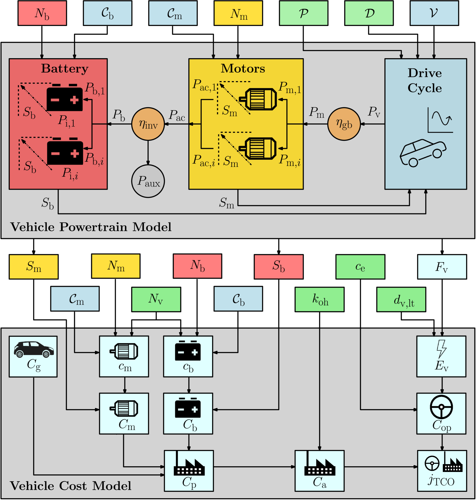
Figure 3: Flow diagram explaining the algorithm employed in computing the objective function (TCO) of our concurrent design optimization framework.

II-C1 Longitudinal Dynamics

We optimize the design of the vehicles for a given driving cycle $\mathcal{D}$ of length $d$ with exogenous longitudinal speed, acceleration, and slope trajectories $v(t)$, $a(t)$, and $\theta(t)$. Hence, the required power at the wheels $P_{\mathrm{v}}$ can be expressed as

$$P_{\mathrm{v},i}=m_{i}\cdot v\cdot\left(c_{\mathrm{r},i}\cdot g\cdot\cos(\theta)+g\cdot\sin(\theta)+a\right)+\\ +\frac{1}{2}\cdot\rho\cdot c_{\mathrm{d},i}\cdot A_{\mathrm{f},i}\cdot v^{3},$$ (17)

where $m_{i}$ is the total mass of each vehicle, $g$ is the gravitational acceleration, $\rho$ is the density of the air, $c_{\mathrm{d},i}$ is the aerodynamic drag coefficient, and $c_{\mathrm{r},i}$ is the rolling resistance coefficient.

II-C2 Mass

The vehicle’s mass $m_{i}$ consists of several contributions: the glider mass $m_{\mathrm{g},i}$, the constant driver mass $m_{\mathrm{d}}$, the payload mass $m_{\mathrm{p},i}$, and the motor and battery mass, computed by scaling $m_{\mathrm{m,o}}$ and $m_{\mathrm{b,o}}$, accounting for the number of modules

$$m_{i}=m_{\mathrm{g},i}+m_{\mathrm{d}}+m_{\mathrm{p},i}+m_{\mathrm{m.o}}\cdot S_{\mathrm{m}}\cdot N_{\mathrm{m},i}+m_{\mathrm{b,o}}\cdot S_{\mathrm{b}}\cdot N_{\mathrm{b},i}.$$ (18)

II-C3 Transmission

We assume that the required power at the wheels $P_{\mathrm{req}}$ is equally divided among the $N_{\mathrm{m}}$ motor modules through fixed-gear transmissions (Fig. 4), whereby we consider the gear ratio $\gamma$ specifically designed for the motor speed interval considered. The transmissions introduce losses that we model via a constant efficiency $\eta_{\mathrm{gb}}$:

$$P_{\mathrm{m},i}=\begin{cases}\frac{P_{\mathrm{v},i}}{\eta_{\mathrm{gb}}\cdot N_{\mathrm{m},i}}\quad&\text{if }P_{\mathrm{req},i}\geq 0\\ r_{\mathrm{b},i}\cdot\frac{\eta_{\mathrm{gb}}\cdot P_{\mathrm{v},i}}{N_{\mathrm{m},i}}\quad&\text{if }P_{\mathrm{req},i}<0\end{cases},$$

$$r_{\mathrm{b},i}=\begin{cases}r_{\mathrm{FWD}}\quad&\text{if FWD}\\ r_{\mathrm{AWD}}\quad&\text{if AWD}\end{cases},$$

where the parameter $r_{\mathrm{b}}$ accounts for the regenerative braking capabilities of the vehicle’s topology $r_{\mathrm{FWD}}$ and $r_{\mathrm{AWD}}$, included in the set $\mathcal{C_{\mathrm{m}}}$. We can relax this constraint to an inequality without changing the problem solution (lossless relaxation) as

$$P_{\mathrm{m},i}\geq\frac{P_{\mathrm{v},i}}{\eta_{\mathrm{gb}}\cdot N_{\mathrm{m},i}},$$ (19)

$$P_{\mathrm{m},i}\geq r_{\mathrm{b},i}\cdot\frac{\eta_{\mathrm{gb}}\cdot P_{\mathrm{v},i}}{N_{\mathrm{m},i}}.$$ (20)

In fact, thanks to the particular problem structure, the optimal solution is located on the boundary, implying that these constraints will always hold with equality [48]. Ultimately, assuming any value higher than the strictly necessary would be sub-optimal since it would entail higher losses and thus additional costs.

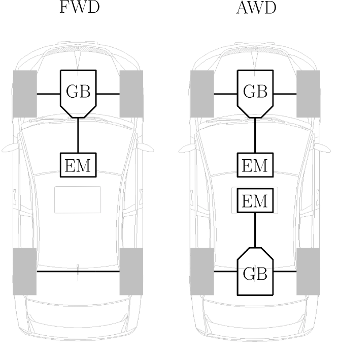
Figure 4: Vehicle topologies considered in this framework: Front-wheel drive (FWD) for vehicles equipping one motor module, and All-wheel drive (AWD) for two.

II-C4 Electric Motor

Analogously to our previous work [34], we make use of a second-order polynomial approximation of the reference motor losses $P_{\mathrm{m,o,loss}}$, extending a quadratic approximation [47] to retain accuracy, without losing convexity

$$P_{\mathrm{m,o,loss}}=P_{\mathrm{0}}(\omega)+\beta(\omega)\cdot P_{\mathrm{m,o}}+\alpha(\omega)\cdot P_{\mathrm{m,o}}^{2}.$$

Furthermore, we assume that the operational limits $\underline{P}_{\mathrm{m,o}}$ and $\overline{P}_{\mathrm{m,o}}$ scale linearly with respect to the reference values

$$P_{\mathrm{m},i}\in\left[\underline{P}_{\mathrm{m,o}},\overline{P}_{\mathrm{m,o}}\right]\cdot S_{\mathrm{m}}.$$ (21)

Following the same rationale, we can write $P_{\mathrm{m,loss}}$ for every motor module as

$$P_{\mathrm{m,loss},i}=\left(P_{\mathrm{0}}(\omega)+\beta(\omega)\cdot\frac{P_{\mathrm{m},i}}{S_{\mathrm{m}}}+\alpha(\omega)\cdot\frac{P_{\mathrm{m},i}^{2}}{S_{\mathrm{m}}^{2}}\right)\cdot S_{\mathrm{m}},$$

yielding

$$P_{\mathrm{m,loss},i}=P_{\mathrm{0}}(\omega)\cdot S_{\mathrm{m}}+\beta(\omega)\cdot P_{\mathrm{m},i}+\alpha(\omega)\cdot\frac{P_{\mathrm{m},i}^{2}}{S_{\mathrm{m}}}.$$

Finally, we obtain the AC input motor power $P_{\mathrm{ac},i}$ equation

$$P_{\mathrm{ac},i}=\left(P_{\mathrm{m},i}+P_{\mathrm{m,loss},i}\right),$$

and we replace the expression for the losses

$$P_{\mathrm{ac},i}=P_{\mathrm{m},i}+P_{\mathrm{0}}(\omega)\cdot S_{\mathrm{m}}+\beta(\omega)\cdot P_{\mathrm{m},i}+\alpha(\omega)\cdot\frac{P_{\mathrm{m},i}^{2}}{S_{\mathrm{m}}}.$$

Analogously to what has been done in Eq. (19), this equation can be losslessly relaxed for the purpose of retaining convexity, obtaining the second-order conic constraint

$$\left(P_{\mathrm{ac},i}-P_{\mathrm{m},i}-S_{\mathrm{m}}\cdot P_{\mathrm{0}}(\omega)-\beta(\omega)\cdot P_{\mathrm{m},i}\right)+\frac{S_{\mathrm{m}}}{\alpha(\omega)}\geq$$

$$\left\|\begin{matrix}2\cdot P_{\mathrm{m},i}\\ \left(P_{\mathrm{ac},i}-P_{\mathrm{m},i}-S_{\mathrm{m}}\cdot P_{\mathrm{0}}(\omega)-\beta(\omega)\cdot P_{\mathrm{m},i}\right)-\frac{S_{\mathrm{m}}}{\alpha(\omega)}\end{matrix}\right\|_{2}.$$ (22)

II-C5 Battery

Similarly to what has been implemented for the EM, for each vehicle of the $i$-th type, every module’s output battery power $P_{\mathrm{b},i}$ can be found starting from $P_{\mathrm{ac},i}$ by considering the inverter efficiency $\eta_{\mathrm{inv}}$, power consumption of auxiliary systems $P_{\mathrm{aux},i}$ (heating, air conditioning, lights, etc.), and motor and battery modules’ multiplicity $N_{\mathrm{m},i}$ and $N_{\mathrm{b},i}$. Following the assumption that every module supplies an equal amount of output power in the $i$-th vehicle,

$$P_{\mathrm{b},i}=\begin{cases}\frac{1}{N_{\mathrm{b},i}}\cdot\left(\frac{P_{\mathrm{ac},i}\cdot N_{\mathrm{m},i}}{\eta_{\mathrm{inv}}}+P_{\mathrm{aux},i}\right)\quad&\text{if }P_{\mathrm{ac},i}\geq 0\\ \frac{1}{N_{\mathrm{b},i}}\cdot\left(\eta_{\mathrm{inv}}\cdot P_{\mathrm{ac},i}\cdot N_{\mathrm{m},i}+P_{\mathrm{aux},i}\right)\quad&\text{if }P_{\mathrm{ac},i}<0\end{cases},$$

that can be relaxed to

$$P_{\mathrm{b},i}\geq\frac{1}{N_{\mathrm{b},i}}\cdot\left(\frac{P_{\mathrm{ac},i}\cdot N_{\mathrm{m},i}}{\eta_{\mathrm{inv}}}+P_{\mathrm{aux},i}\right),$$ (23)

$$P_{\mathrm{b},i}\geq\frac{1}{N_{\mathrm{b},i}}\cdot\left(\eta_{\mathrm{inv}}\cdot P_{\mathrm{ac},i}\cdot N_{\mathrm{m},i}+P_{\mathrm{aux},i}\right).$$ (24)

We model the battery’s internal losses using a function of the power that the battery would release when short-circuited: the “short circuit power” [34] $P_{\mathrm{sc},i}$. We make use of a convex piece-wise affine approximation of the function composed of $K$ parts, depending on the energy $E_{\mathrm{b},i}$ and size $S_{\mathrm{b}}$ [47]. Hence, for every battery module,

$$P_{\mathrm{i},i}=P_{\mathrm{b},i}+\frac{P_{\mathrm{i},i}^{2}}{P_{\mathrm{sc},i}},$$

where

$$P_{\mathrm{sc},i}=\min_{k\in\{1,...,K\}}\left\{a_{k}\cdot E_{\mathrm{b},i}+b_{k}\cdot S_{\mathrm{b}}\right\}.$$

However, the form of this constraint would not allow a convex formulation, therefore, we apply a lossless relaxation to treat a set of affine inequalities.

$$P_{\mathrm{sc},i}\leq a_{k}\cdot E_{\mathrm{b},i}+b_{k}\cdot S_{\mathrm{b}}\;\forall k.\in\{1,...,K\}.$$ (25)

Following the same logic applied in Section II-C4, we also relax the battery losses equation to

$$\left(P_{\mathrm{i},i}-P_{\mathrm{b},i}\right)+P_{\mathrm{sc},i}\geq\left\|\begin{matrix}2\cdot P_{\mathrm{i},i}\\ \left(P_{\mathrm{i},i}-P_{\mathrm{b},i}\right)-P_{\mathrm{sc},i}\end{matrix}\right\|_{2}.$$ (26)

The overall energy of the battery $E_{\mathrm{tot},i}$ is determined by each module’s size and the total number of modules per vehicle

$$E_{\mathrm{tot},i}\in\left[\ \overline{E}_{\mathrm{b,o}}\cdot\underline{\xi},\overline{E}_{\mathrm{b,o}}\cdot\overline{\xi}\ \right]\cdot S_{\mathrm{b}}\cdot N_{\mathrm{b},i},$$ (27)

while the dynamic of $E_{\mathrm{tot},i}$ is influenced by the internal power via

$$\frac{\mathrm{d}E_{\mathrm{tot},i}}{\mathrm{d}t}=-N_{\mathrm{b}}\cdot P_{\mathrm{i},i}.$$ (28)

Ultimately, we evaluate the distance-specific energy consumption $F_{\mathrm{v},i}$ by dividing $E_{\mathrm{tot},i}$ by driving cycle length $d$

$$F_{\mathrm{v},i}=\frac{E_{\mathrm{tot},i}(0)-E_{\mathrm{tot},i}(T)}{d}.$$ (29)

Since we consider a variable efficiency of the battery through $P_{\mathrm{sc},i}$, we include a constraint to ensure that the operations are conducted around the half-capacity level of the battery by averaging the maximum capacity at the start and the minimum capacity at the end of the driving cycle

$$E_{\mathrm{tot},i}(0)=S_{\mathrm{b}}\cdot\overline{\xi}\cdot\overline{E}_{\mathrm{b,o}}\cdot N_{\mathrm{b},i},$$

$$E_{\mathrm{tot},i}(T)=S_{\mathrm{b}}\cdot\underline{\xi}\cdot\overline{E}_{\mathrm{b}}\cdot N_{\mathrm{b},i},$$

$$E_{\mathrm{tot},i}(0)+E_{\mathrm{tot},i}(T)=S_{\mathrm{b}}\cdot\left(\overline{\xi}+\underline{\xi}\right)\cdot\overline{E}_{\mathrm{b,o}}\cdot N_{\mathrm{b},i}.$$ (30)

II-C6 Performance Constraints

Besides the equations modeling the powertrain behavior during vehicles’ operations, we include constraints on the performance of each vehicle. Hence, we write in convex form the acceleration time, top speed, power gradability, torque gradability, and range constraints as

$$N_{\mathrm{m},i}\cdot S_{\mathrm{m}}\cdot t_{\mathrm{a},i}\leq\frac{\omega_{\mathrm{r}}\cdot r_{\mathrm{w},i}^{2}\cdot m_{i}}{\overline{T}_{\mathrm{m,o}}\cdot\gamma^{2}}+\frac{m_{i}\cdot\left(v_{\mathrm{f}}^{2}+\frac{\omega_{\mathrm{r}}^{2}}{\gamma^{2}}\cdot r_{\mathrm{w},i}^{2}\right)}{2\cdot\overline{P}_{\mathrm{m,o}}},$$ (31)

$$N_{\mathrm{m},i}\cdot S_{\mathrm{m}}\cdot\overline{P}_{\mathrm{m,o}}\geq\frac{1}{2}\cdot\rho\cdot c_{\mathrm{d},i}\cdot A_{\mathrm{f},i}\cdot\left(v_{\mathrm{t},i}\right)^{3},$$ (32)

$$N_{\mathrm{m},i}\cdot S_{\mathrm{m}}\cdot\overline{P}_{\mathrm{m},o}\geq m_{i}\cdot g\cdot v_{\mathrm{m},i}\cdot\sin(\theta_{i}),$$ (33)

$$N_{\mathrm{m},i}\cdot S_{\mathrm{m}}\cdot\overline{T}_{\mathrm{m,o}}\cdot\gamma\geq m_{i}\cdot g\cdot r_{\mathrm{w},i}\cdot\sin(\theta_{i}),$$ (34)

$$E_{\mathrm{tot},i}(0)-E_{\mathrm{tot},i}(T)\leq N_{\mathrm{b},i}\cdot S_{\mathrm{b}}\cdot\left(\overline{\xi}-\underline{\xi}\right)\cdot\overline{E}_{\mathrm{b,o}}\cdot\frac{d}{d_{\mathrm{r},i}},$$ (35)

where $\overline{T}_{\mathrm{m,o}}$ is the maximum reference torque

$$\overline{T}_{\mathrm{m,o}}=\frac{\overline{P}_{\mathrm{m,o}}}{\omega_{\mathrm{r}}}.$$

The values of the acceleration time $t_{\mathrm{a},i}$, top speed $v_{\mathrm{t},i}$, uphill speed $v_{\mathrm{m},i}$, slope $\theta_{i}$, and range $d_{\mathrm{r},i}$ are bounded by the required performance in the set $\mathcal{P}$

$$t_{\mathrm{a},i}<=\overline{t}_{\mathrm{a},i},$$ (36)

$$v_{\mathrm{t},i}>=\underline{v}_{\mathrm{t},i},$$ (37)

$$v_{\mathrm{m},i}>=\underline{v}_{\mathrm{m},i},$$ (38)

$$\theta_{i}>=\underline{\theta}_{i},$$ (39)

$$d_{\mathrm{r},i}>=\underline{d}_{\mathrm{r},i}.$$ (40)

II-D Optimization Problem Formulation

We formulate the concurrent design optimization problem with the objective of minimizing the TCO of the vehicle family by choosing the sizing of the shared modules and their multiplicity as follows.

Problem 1 (Concurrent Design Optimization Problem).

Given a family of battery electric vehicles with modular powertrains, the TCO-optimal shared modules’ sizes and multiplicity for the whole family are the solution of

$$\qquad\min_{S_{\mathrm{m}},S_{\mathrm{b}},N_{\mathrm{m},i},N_{\mathrm{b},i}}J_{\mathrm{TCO}}$$

s.t. Shared Constraints (1)-(6)

      Vehicle Constraints (8)-(40) $$\forall k\quad\forall i$$

This problem can be solved with global optimality guarantees in a nested fashion: For given $N_{\mathrm{m},i}$ and $N_{\mathrm{b},i}$, this problem can be framed as a second-order conic program and rapidly solved to global optimality with standard algorithms. Thus, we analyze each of the $N_{\mathrm{c}}$ possible configurations

$$N_{\mathrm{c}}=\left(\lvert\mathbb{M}\rvert\cdot\lvert\mathbb{B}\rvert\right)^{N},$$

leveraging the polynomial solving time of the convex approach, and identify the globally optimal solution through an exhaustive search.

II-E Discussion

A few comments are in order. First, we conservatively assumed that every vehicle has a fixed percentage of overhead costs, yet the methodology is still sound for every cost model incorporating the effect of EoS. Second, we scale the electric motor mass linearly as a function of the maximum power and the battery size only by acting on the number of cells in parallel, thus changing its energy without altering the battery voltage. These scaling methods are in line with high-level modeling approaches and optimal sizing design problems. Third, we assume that every vehicle is equipped with the same transmission modules. The gear ratio $\gamma$ is considered to be specifically designed for the motor speed range, which remains constant while linearly scaling the motor in torque. For a fair comparison, $\gamma$ is kept constant both in the individual vehicle-tailored design and in the concurrent design optimization. This assumption is in accordance with the common design practice among electric vehicle manufacturers of using a standard reduction gear. Finally, the problem could be solved as a Mixed Integer Second Order Conic Program (MISOCP) instead of applying a nested approach. Nevertheless, we leverage the fast solving time of convex programs to retain information on the other sub-optimal configurations, additionally obtaining sensitivity information.

III Results

In this section, we showcase our methodology with a benchmark design problem considering the family design of four different Tesla models: Model S, Model 3, Model X and Model Y. We compare the results of the concurrent strategy with a vehicle-tailored design optimization, whereby the modules’ sizes are optimized individually for a single vehicle. The vehicle-tailored design is computed with the same framework considering only one vehicle at the time, with $N_{\mathrm{b}}=1$ and $N_{\mathrm{m}}=2$ (AWD topology). In order to minimize the errors owing to market fluctuations, we adjusted the figures for inflation [49] and converted the dollars into euros where necessary [50]. In our analyses, we refer to market and technology from the year 2020. Table I gathers the parameters used for the cost model, Table III shows the reference parameters of the modules, whereas Table II contains vehicle parameters, performance parameters, and vehicle type fractions.

TABLE I: Cost model parameters [51, 52, 53]

Parameter	Value	Unit
$c_{\mathrm{b},2020}$	79	EUR/kWh
$\lambda_{\mathrm{b,1}}$	3911	EUR/kWh
$\lambda_{\mathrm{b,2}}$	0.3278	-
$c_{\mathrm{m},2020}$	2.2	EUR/kWh
$\lambda_{\mathrm{m,1}}$	537	EUR/kWh
$\lambda_{\mathrm{m,2}}$	0.4524	-
$C_{\mathrm{e}}$	0.4	EUR/kWh
$N_{\mathrm{v}}$	200000	-
$d_{\mathrm{v,lf}}$	200000	km
$k_{\mathrm{oh}}$	0.5350	-
$C_{\mathrm{g}}$	14736	EUR

TABLE II: Parameters from sets $\mathcal{V}$,$\mathcal{P}$,$\mathcal{W}$ [54, 55]

Tesla	Model S	Model 3	Model X	Model Y	Unit
$m_{\mathrm{g}}$	1105	1069	1328	1205	kg
$\eta_{\mathrm{gb}}$	0.98	0.98	0.98	0.98	-
$\eta_{\mathrm{inv}}$	0.96	0.96	0.96	0.96	-
$A_{\mathrm{f}}$	2.34	2.2	2.59	2.66	m^2
$c_{\mathrm{d}}$	0.24	0.23	0.24	0.23	-
$r_{\mathrm{w}}$	0.3518	0.3353	0.3759	0.3560	m
$c_{\mathrm{r}}$	0.007	0.007	0.007	0.007	-
$m_{\mathrm{p}}$	0	0	500	500	kg
$m_{\mathrm{d}}$	80	80	80	80	kg
$P_{\mathrm{aux}}$	500	500	500	500	W
$\overline{t}_{\mathrm{a}}$	3.3	6.1	3.9	6.9	s
$\underline{v}_{\mathrm{f}}$	100	100	100	100	km/h
$\underline{v}_{\mathrm{t}}$	261	225	262	217	km/h
$\underline{v}_{\mathrm{m}}$	10	10	10	10	km/h
$\underline{\theta}$	25	25	25	25	%
$\underline{d}_{\mathrm{r}}$	460	405	455	350	km
$w$	0.25	0.25	0.25	0.25	-

TABLE III: Reference motor and battery parameters

Symbol	Value	Unit
$\mathbb{M}$	$\left\{1,2\right\}$	-
$\overline{S}_{\mathrm{m}}$	4	-
$\underline{S}_{\mathrm{m}}$	0.25	-
$\gamma$	9.01	-
$m_{\mathrm{m,o}}$	81.6	kg
$\overline{P}_{\mathrm{m,o}}$	89.38	kW
$\omega_{\mathrm{r}}$	418.88	rad/s
$r_{\mathrm{FWD}}$	0.6	-
$r_{\mathrm{AWD}}$	1	-
$\mathbb{B}$	$\left\{1,2,3\right\}$	-
$\overline{S}_{\mathrm{b}}$	4	-
$\underline{S}_{\mathrm{b}}$	0.25	-
$m_{\mathrm{b,o}}$	138.6	kg
$\overline{E}_{\mathrm{b,o}}$	23.48	kWh
$\overline{\xi}$	0.9	-
$\underline{\xi}$	0.1	-

We consider the Class 3 Worldwide harmonized Light-duty vehicles Test Procedure (WLTP) for the speed and acceleration trajectories and we discretize Problem 1 using the Euler forward method with a sampling time of 1 s. Thereafter, we parse it with YALMIP [56] and solve it to global optimality with MOSEK [57], in 2 s for each of the possible $N_{\mathrm{c}}$ combinations. It is important to underline that the solution depends on the sets $\mathbb{M}$ and $\mathbb{B}$. In fact, they influence the possible ratios of motor power and battery capacity among the vehicles, thus potentially increasing efficiency and lowering costs. Also, having more elements in the sets means a higher number of possible configurations, therefore increasing the total computation time. Finally, in our benchmark problem, we consider equal fractions of vehicles of the $i$-th type, i.e., $w_{i}=25\%$. These parameters act like weights in the optimization, determining the vehicle types’ importance according to the market research outcome.

Fig. 5 shows the comparison of the TCO achieved by concurrent and tailored design optimization for an energy price 40 EUR cents per kWh, and 200 thousand vehicles, highlighting that sizing the powertrain modules for the benchmark problem using a concurrent design optimization approach achieves a reduction of the Family TCO of 3.5% compared to the individual vehicle-tailored optimization.

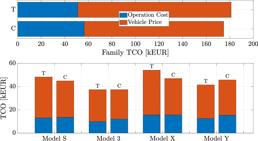
Figure 5: Comparison of costs between the concurrent design optimization (C) and the individual vehicle-tailored design (T). The bars on the top of the picture depict the overall TCO of the family, showing a slight increment in operation cost against a significant reduction of the vehicle selling price. Below we show the single contribution of each vehicle.

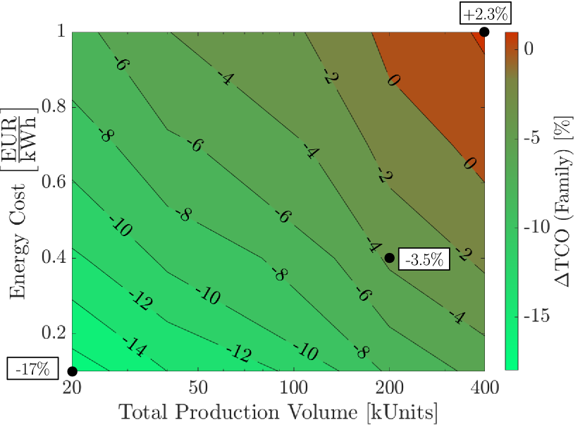
Figure 6: Profitability map of the concurrent design optimization approach for different market conditions of energy prices and production volumes. It is especially beneficial to share family-optimal modules for cheap energy prices and for small-scale production volumes.

Specifically, there is an advantageous trade-off in using standardized modules to significantly reduce the cost of manufacturing while observing a limited increase in the operation costs thanks to the higher versatility prompted by modularity. Interestingly, whilst always beneficial to the manufacturer, the family-optimal design could be disadvantageous to some users, ending up with a higher TCO compared to its vehicle-tailored design if it leads to a greater cost reduction for the rest of the family (Model Y in Fig. 5). Table IV reports the family design and performance specification of the concurrent design optimized family compared to its vehicle-tailored counterpart.

TABLE IV: Benchmark problem family design specifications compared to a vehicle-tailored design

Tesla	Model S	Model 3	Model X	Model Y	Unit
$j_{\mathrm{TCO}}$	44884	37381	46950	45730	EUR
$\Delta$	-6.98	+0.04	-13.28	+10.22	%
$m$	2232	1784	2455	2142	kg
$\Delta$	+6.57	+7.57	+0.60	+16.31	%
$d_{\mathrm{r}}$	533	405	462	471	km
$\Delta$	+15.88	0.00	+1.66	+34.62	%
$t_{\mathrm{a}}$	3.28	4.96	3.90	6.38	s
$\Delta$	-0.71	-18.72	=0.00	-7.60	%
$v_{\mathrm{t}}$	436	359	422	337	km/h
$\Delta$	+2.39	+9.79	+0.20	+7.97	%
$F_{\mathrm{v}}$	0.6101	0.5354	0.7031	0.6903	MJ/km
$\Delta$	+3.66	+21.61	+0.24	+22.13	%
$\overline{P}_{\mathrm{tot}}$	625	313	625	313	kW
$\Delta$	+7.33	+32.33	+0.60	+25.87	%
$\overline{E}_{\mathrm{tot}}$	113	75	113	113	kWh
$\Delta$	+20.12	+21.61	+1.91	+64.42	%
$S_{\mathrm{m}}$	2.33 (312 kW)				-
$\Delta$	+7.33	+164.67	+0.60	+151.75	%
$S_{\mathrm{b}}$	1.60 (37.64 kWh)				-
$\Delta$	-59.96	-39.20	-66.03	-45.19	%
$N_{\mathrm{m}}$	2	1	2	1	-
$\Delta$	0	-50	0	-50	%
$N_{\mathrm{b}}$	3	2	3	3	-
$\Delta$	+200	+100	+200	+100	%

We examine the sensitivity of the solution to different market conditions like energy price and production volume in Fig. 6. We consider electricity prices for household consumers in line with the statistics in the Netherlands [52, 51] and other European countries [53]. The electricity price linearly influences the operation cost, increasing the profitability of the concurrent design optimization methodology for affordable energy, whereby this strategy leverages a trade-off between energy efficiency and component costs. Furthermore, the relative profitability of the concurrent optimization methodology grows with decreasing production volumes up to a maximum theoretical limit, achieved for 1 unit per type produced. Since the absolute saving in production cost grows asymptotically with production volumes (law of diminishing returns), the maximum theoretical limit does not have a practical application. Therefore, in Fig. 6 we show typical production volumes of electric vehicle manufacturers from data of the latest years [58]. Hence, on the one hand, employing a shared modular design is always advantageous for the vehicle manufacturer, who aims to produce as much as possible to leverage the cost reduction fostered by the economy of scale. On the other hand, the final user of the vehicle will benefit from a reduction in the acquisition price, which outweighs the increment in operation costs of a sub-optimal energy-efficiency family design. Above a certain threshold, depending on the production volumes, this trade-off is no longer beneficial, and an individual vehicle-tailored design is more favorable.

IV Conclusions

This paper presented a concurrent design optimization framework to identify the family-optimal size and multiplicity configuration of motor and battery modules that are shared within a family of electric vehicles, explicitly accounting for economy of scale effects. To this end, we devised a cost model capturing the influence of production volumes, energy cost, modules’ size and multiplicity on the vehicle’s Total Cost of Ownership (TCO), and a powertrain model to account for its operations. The resulting framework enables to compute minimum-TCO vehicle family design solutions with global optimality guarantees. When applied to a real-world case-study for the design of the Tesla vehicle family, our methodology achieves a reduction of 3.5% in the family TCO compared to vehicle-tailored design solutions, whilst maintaining outstanding performance. However, the profitability of the approach ranges from a saving in family TCO of 17% for cheap energy prices and small production volumes to an increase of 2.3% for very expensive energy and large production volumes, where the increase in production brought by sharing modules minimally reduces the production costs, due to the asymptotic behavior of the cost function. Overall, concurrent design optimization proved to be advantageous for a wide range of volumes and electricity prices, creating an opportunity to support the transition to electric mobility by substantially reducing the vehicle’s upfront cost, one of the major factors hindering its adoption.

This work opens the field for the following extensions: First, we aim to sophisticate the framework by incorporating the optimization of the transmission and more powertrain architectures. Second, we would like to assess the vehicles’ environmental impact via life cycle analysis, and study the effect of its minimization on the design solutions.

Appendix A Cost Model

After a careful review of the literature, we developed a cost model able to portray the influence of EoS strategies on battery packs and motor costs. We report the data [39, 40, 59, 60, 61, 62] used to identify $c_{\mathrm{b},2020}$, $\lambda_{\mathrm{b,1}}$, $\lambda_{\mathrm{b,2}}$, $c_{\mathrm{m},2020}$, $\lambda_{\mathrm{m,1}}$, and $\lambda_{\mathrm{m,2}}$ in Table VI, portraying the identified functions in Figures 8 and 8. Furthermore, we indicate the glider cost depending on the vehicle type in Table VII. Finally, we compute the selling price from the manufacturing cost by considering the overhead costs to be a constant fraction [35] $k_{\mathrm{oh}}$, as shown in Fig. 10. The prediction of the cost model has been validated with a set of different BEVs, achieving good results in modeling vehicle price using just the vehicle type, battery capacity, and motor power, assuming an average hundred thousand vehicles produced (Table V and Fig. 9). However, the error in the prediction increases for luxury brands, where the price is heavily influenced by factors which are not strongly coupled with manufacturing.

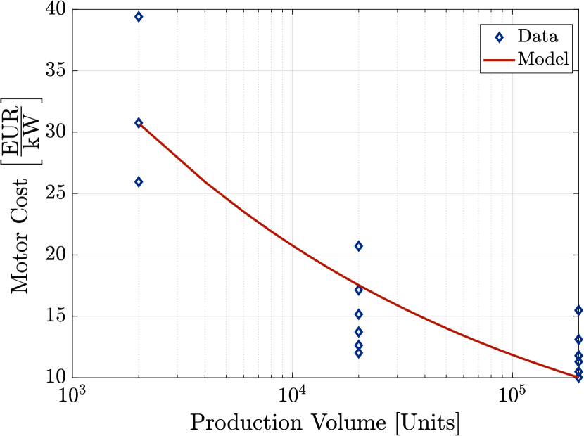
Figure 7: Production volumes impact on the motor cost in Euro per kW.

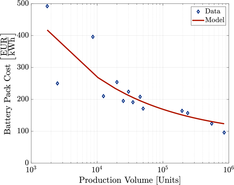
Figure 8: Production volumes impact on the battery pack cost in Euro per kWh.

TABLE V: Validation of the vehicle’s cost model assuming an average production volume of a hundred thousand vehicles per type

Vehicle	Capacity	Power	Pred.	Price
	kWh	kW	EUR	EUR
City (Seg. A-B)
Mitsubishi i-MiEV	16	47	20188	19990 [63]
Peugeot iOn	16	47	20188	22360 [64]
Citroen C-Zero	16	47	20188	21800 [64]
Smart EQ fortwo	17.6	60	20746	23995 [64]
Renault Twingo E	23	60	22450	22105 [65]
Dacia Spring Electric	26.8	33	23537	21750 [66]
Opel Corsa-e	50	100	31134	30999 [67]
Peugeot e-208	50	100	31134	33220 [68]
Renault Zoe Q90	52	100	31765	33590 [64]
Compact (Seg. C)
Nissan Leaf	40	110	33222	35090 [64]
Citroen e-C4 X	50	100	36336	40140 [69]
ORA Funky Cat Ied	51	126	36758	38990 [64]
Renault Zoe R135	52	100	36967	36295 [64]
Kia Niro EV	68	150	42221	43850 [70]
Large (Seg. D-E)
Tesla Model 3	60	208	47333	42993 [54]
Tesla Model Y	60	220	47382	47993 [54]
Polestar 2	69	200	50222	51200 [71]
Polestar 2 LR	82	220	54324	55200 [71]
Polestar 2 Dual LR	82	310	54695	59900 [71]

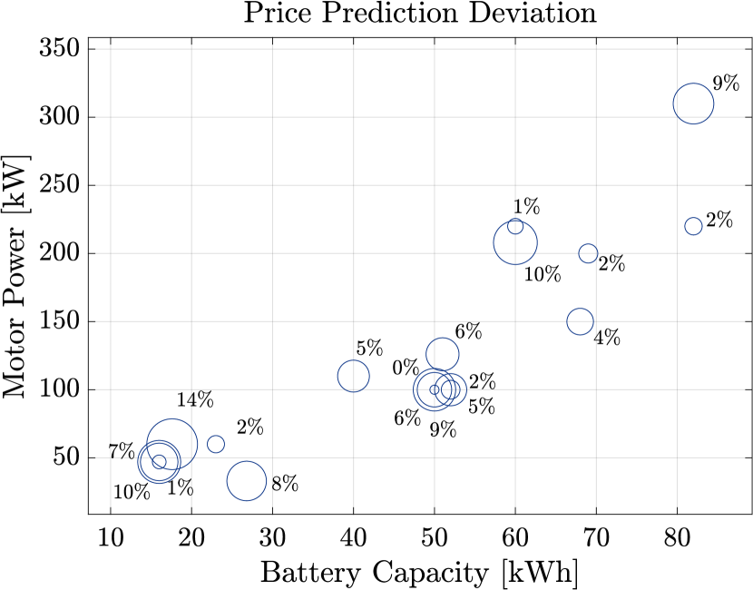
Figure 9: Percentage deviation of the model prediction from vehicles’ price.

TABLE VI: Peak-power-specific cost by production volumes [72, 73] (left), and Battery Pack capacity-specific cost by production volumes [35, 46, 74] (right)

Motor	Cost	Battery Pack	Cost
Units	[EUR/kW(p)]	Units	[EUR/kWh]
2000	39.40	1750	492
2000	30.75	2500	250
2000	25.95	8625	396
20000	20.71	12500	210
20000	17.14	20000	254
20000	15.15	25000	195
20000	13.72	30000	224
20000	12.62	35000	191
20000	12.01	45000	208
200000	15.48	50000	171
200000	13.10	95000	164
200000	11.78	237500	157
200000	11.29	550000	124
200000	10.47	850000	96
200000	10.02

TABLE VII: Glider Costs in 2020 [38, 75]

Vehicle Type	Glider Cost [EUR]
City Cars	7996
Compact Cars	10779
Large Cars	14736

Figure 10: Price breakdown of a new vehicle [35, 43].

References

- [1] IEA, “Global EV outlook 2021,” International Energy Agency, Tech. Rep., 2021.
- [2] E. McTurk, “Do electric vehicles produce more tyre and brake pollution than petrol and diesel cars?” Plug Life Consulting for the RAC, Tech. Rep., 2022.
- [3] IEA, “Global EV outlook 2020,” International Energy Agency, Tech. Rep., 2020.
- [4] UNEP and D. Partnership, “Emissions gap report 2021: The heat is on – a world of climate promises,” United Nations Environment Programme and Technical University of Denmark, Tech. Rep., 2021.
- [5] IEA, “Global EV outlook 2022,” International Energy Agency, Tech. Rep., 2022.
- [6] L. Paoli. (2022) Electric cars fend off supply challenges to more than double global sales,. Paris. International Energy Agency. Https://www.iea.org/commentaries/electric-cars-fend-off-supply-challenges-to-more-than-double-global-sales.
- [7] Avicenne Energy, “European Union and UK Automotive ICE vs EV Total Cost of Ownership,” Nickel Institute, Tech. Rep., 2021.
- [8] Lightyear. (2022) Producing worldś most efficient car to date, under every weather condition and speed. Online. Lightyear. Https://lightyear.one/articles/producing-worlds-most-efficient-car-to-date-under-every-weather-condition-and-speed.
- [9] K. Medini, A. Pierné, J. A. Erkoyuncu, and C. Cornet, “A Model for Cost-Benefit Analysis of Production Ramp-up Strategies,” in Proc. of Advances in Production Management Systems, B. Lalic, V. Majstorovic, U. Marjanovic, G. von Cieminski, and D. Romero, Eds. Springer International Publishing, 2020, pp. 731–739.
- [10] Advanced Manufacturing Office, “Improving motor and drive system performance,” US Department of Energy: Energy Efficiency & Renewable Energy, Tech. Rep., 2014.
- [11] J. Jiao, T. W. Simpson, and Z. Siddique, “Product family design and platform-based product development: a state-of-the-art review,” Journal of Intelligent Manufacturing, vol. 18, no. 1, pp. 5–29, 2007.
- [12] D. Robertson and K. Ulrich, “Planning for product platforms,” The Wharton Annual, vol. 39, no. 4, pp. 19–31, 1998.
- [13] K. Otto, K. Hölttä-Otto, T. W. Simpson, D. Krause, S. Ripperda, and S. K. Moon, “Global views on modular design research: Linking alternative methods to support modular product family structure design,” ASME Journal of Mechanical Design, vol. 138, no. 7, p. 071101, 2016.
- [14] T. W. Simpson, Z. Siddique, and J. Jiao, Product Platform and Product Family Design Methods and Applications, 1st ed. Springer US, 2006.
- [15] S. W. Sanderson and M. Uzumeri, “Managing product families: The case of the sony walkman,” Research Policy, vol. 24, no. 5, pp. 761–782, 1995.
- [16] ——, Managing Product Families, 2nd ed. McGraw-Hill Publishing Co., 1997.
- [17] K. Sabbagh, Twenty-First Century Jet: The Making and Marketing of the Boeing 777, 1st ed. Scribner, 1996, new York, NY.
- [18] R. Rothwell and P. Gardiner, Robustness and Product Design Families, 1st ed. Basil Blackwell Inc., Cambridge MA, 1990, ch. Design Management: A Handbook of Issues and Methods, pp. 279–292.
- [19] R. T. Caffrey, T. W. Simpson, R. Henderson, and E. Crawley, “The Technical Issues with Implementing Open Avionics Platforms for Spacecraft,” in 40th AIAA Aerospace Sciences Meeting, 2022.
- [20] R. Bremmer, “Cutting-Edge Platforms,” Financial Times Automotive World, vol. 1999, no. 6, pp. 30–38, 1999.
- [21] ——, “Big, Bigger, Biggest,” Automotive World, vol. 2000, no. 6, pp. 36–44, 2000.
- [22] K. Nobeoka and M. A. Cusumano, Thinking Beyond Lean: How Multi-project Management is Transforming Product Development at Toyota and Other Companies, 1st ed., Simon and Schuster, Eds. Free Press, 1997.
- [23] P. G. Pereirinha and J. P. Trovão, “Standardization in electric vehicles,” in 12th Portuguese-Spanish Conference on Electerical Engineering, 2011.
- [24] L. Guzzella and A. Sciarretta, Vehicle propulsion systems: Introduction to Modeling and Optimization, 2nd ed. Springer Berlin Heidelberg, 2007.
- [25] E. Silvas, T. Hofman, N. Murgovski, P. Etman, and M. Steinbuch, “Review of optimization strategies for system-level design in hybrid electric vehicles,” IEEE Transactions on Vehicular Technology, vol. 66, no. 1, pp. 57–70, 2016.
- [26] Z. Wang, J. Zhou, and G. Rizzoni, “A review of architectures and control strategies of dual-motor coupling powertrain systems for battery electric vehicles,” Renewable and Sustainable Energy Reviews, vol. 162, no. 1, p. 112455, 2022.
- [27] T. Hofman and M. Salazar, “Transmission ratio design for electric vehicles via analytical modeling and optimization,” in IEEE Vehicle Power and Propulsion Conference, 2020.
- [28] S. Radrizzani, G. Riva, G. Panzani, M. Corno, and S. S. M., “Optimal sizing and analysis of hybrid battery packs for electric racing cars,” IEEE Transactions on Transportation Electrification, pp. 1–1, 2023.
- [29] F. J. R. Verbruggen, V. Rangarajan, and T. Hofman, “Powertrain design optimization for a battery electric heavy-duty truck,” in Proc. of the American Control Conference, 2019.
- [30] O. Borsboom, C. A. Fahdzyana, T. Hofman, and M. Salazar, “A convex optimization framework for minimum lap time design and control of electric race cars,” IEEE Transactions on Vehicular Technology, vol. 70, no. 9, pp. 8478–8489, 2021.
- [31] D. Da Silva, L. Kefsi, and A. Sciarretta, “Analytical models for the sizing optimization of fuel cell hybrid electric vehicle powertrains,” in 16th International Conference on Engines & Vehicles. IFP Energies Nouvelles Inst. Carnot IFPEN Transports Energie, 2023, pp. 0133–0151.
- [32] O. Borsboom, M. Salazar, and T. Hofman, “Electric motor design optimization: A convex surrogate modeling approach,” in Symposium on Advances in Automotive Control, 2022.
- [33] P. Anselma, “Electric powertrain sizing for vehicle fleets of car makers considering total ownership costs and emission legislation scenario,” Applied Energy, vol. 1, no. 314, p. 118902, 2022.
- [34] M. Clemente, M. Salazar, and T. Hofman, “Concurrent Powertrain Design for a Family of Electric Vehicles,” in 10th Advances in Automotive Control, 2022.
- [35] A. König, L. Nicoletti, D. Schröder, S. Wolff, A. Waclaw, and M. Lienkamp, “An Overview of Parameter and Cost for Battery Electric Vehicles,” World Electric Vehicle Journal, vol. 12, no. 1, pp. 21–50, 2021.
- [36] A. Hoekstra, A. Vijayashankar, and V. Sundrani, “Modelling the Total Cost of Ownership of Electric Vehicles in the Netherlands,” in Proc. of the Int. Symp. on Electric Vehicles 30th edition, 2017.
- [37] S. Simeu and N. Kim, “Standard driving cycles comparison (iea) & impacts on the ownership cost,” in InPreceedings of the SAE World Congress & Exibition, 2018.
- [38] K. Simeu, N. Kim, and B. Dupont. (2021) Bean. Online. Argonne National Laboratory. Https://vms.taps.anl.gov/tools/bean/.
- [39] M. Fries, M. Kerler, S. Rohr, M. Sinning, and M. Lienkamp, “An Overview of Costs for Vehicle Components, Fuels, Greenhouse Gas Emissions and Total Cost of Ownership,” Technische Universität München, Tech. Rep., 2017, update 2017.
- [40] R. Kochhan, S. Fuchs, B. Reuter, P. Burda, S. Matz, and M. Lienkamo, “An Overview of Costs for Vehicle Components, Fuels, Greenhouse Gas Emissions and Total Cost of Ownership,” 2014, 2014.
- [41] A. Brooker, J. Gonder, L. Wang, E. Wood, S. Lopp, and L. Ramroth, “FASTSIM: A Model to Estimate Vehicle Efficiency, Cost and Performance,” SAE Technical Paper, vol. 1, p. 0973, 2015.
- [42] Office of Energy Efficiency and Renewable Energy, “United states industrial electric motor systems market opportunities assessment,” U.S. Department of Energy, Tech. Rep., 1998.
- [43] WirtschaftsWoche. (2014) Zusammensetzung des preises eines neuwagens in deutschland. Online. Statista.
- [44] A. Del Duce, M. Gauch, and H. Althaus, “Electric passenger car transport and passenger car life cycle inventories in ecoinvent version 3,” Int. Journal of Life Cycle Assessment, vol. 2014, no. 21, pp. 1314–1326, 2014.
- [45] I. Barnes, Automotive Gearbox Overhaul Manual, 1st ed. Haynes Manuals Inc., 1998.
- [46] M. Anderman, “Extract from the xEV insider report,” Total Battery Consulting, Tech. Rep., 2019.
- [47] F. J. R. Verbruggen, M. Salazar, M. Pavone, and T. Hofman, “Joint design and control of electric vehicle propulsion systems,” in European Control Conference, 2020.
- [48] S. Ebbesen, M. Salazar, P. Elbert, C. Bussi, and C. H. Onder, “Time-optimal control strategies for a hybrid electric race car,” IEEE Transactions on Control Systems Technology, vol. 26, no. 1, pp. 233–247, 2018.
- [49] Alioth Finance. (2022) Inflation Calculator 1 Dollar in 1991 to 2022. Online. Official Inflation Data. Https://www.officialdata.org/us/inflation/1991?amount=1.
- [50] Google Finance. (2022) USD/EUR conversion. Online. Google. Available: https://www.google.com/finance/quote/USD-EUR?hl=en&window=1M.
- [51] Ministry of Economic Affairs and Climate Policy. (2023) Price cap for gas, electricity and district heating. Online. Government of the Netherlands. Acccessed on 19/09/23.
- [52] Centraal Bureau voor de Statistiek. (2023) Average energy prices for consumers 2018-2023. Online. CBS. Accessed on 04/08/2023.
- [53] Eurostat. (2022) Electricity prices for households in the European Union (eu-27/eu-28) from 1st half 2010 to 1st half 2022 (in euro cents per kilowatt-hour). Online. Statista. Available: https://www.statista.com/statistics/418049/electricity-prices-for-households-in-eu-28/.
- [54] Tesla. (2023) Tesla website. Online. Tesla. Https://www.tesla.com/.
- [55] EVDatabase. (2022) Electric vehicle database. Available at https://ev-database.uk.
- [56] J. Löfberg, “YALMIP : A toolbox for modeling and optimization in MATLAB,” in IEEE Int. Symp. on Computer Aided Control Systems Design, 2004.
- [57] M. ApS. (2017) MOSEK optimization software. Available at https://mosek.com/.
- [58] Tesla. (2023) Number of tesla vehicles produced worldwide from 1st quarter 2016 to 2nd quarter 2023 (in units). Online. Statista. Available: https://www.statista.com/statistics/715421/tesla-quarterly-vehicle-production/.
- [59] K. Rajashekara and R. Martin, “Electric vehicle propulsion systems present and future trends,” Journal of Circuits, Systems, and Computers, vol. 5, no. 1, pp. 109–219, 1995.
- [60] A. Vyas, R. Cuenca, and L. Gaines, “An assessment of electric vehicle life cycle cost to consumers,” SAE Technical Paper, vol. 982182, 1998.
- [61] O. of Technology Assessment, Advanced Automotive Technology: Visions of a Super-Efficient Family Car, C. Clark, Ed. Princeton, 1995.
- [62] J. de Santiago, H. Bernhoff, B. Ekergard, S. Eriksson, S. Ferhatovic, and R. Waters, “Electrical motor drivelines in commercial all electric vehicles: a review,” Transactions of Vehicular Techonologiy, vol. 61, no. 2, pp. 475–484, 2012.
- [63] Autoweek. (2023) Mitsubishi I-MIEV. Online. Autoweek.nl. Https://www.autoweek.nl/auto/59111/mitsubishi-i-miev/.
- [64] Elektrische Voertuigen Database. (2023) EV Database. Online. EV Database. v4.4.
- [65] Autoweek. (2023) Renault twingo electric collection. Online. Autoweek.nl. Https://www.autoweek.nl/auto/100944/renault-twingo-electric-collection/.
- [66] DACIA. (2023) DACIA spring. Online. DACIA Van Mossel. Https://www.vanmossel.nl/dacia/acties/dacia-spring/.
- [67] OPEL. (2023) Opel corsa-e. Online. OPEL. Https://www.opel.nl/personenwagens/corsa-modellen/corsa-electric/overzicht.html.
- [68] Peugeot. (2023) Peugeot official website. Online. Peugeot. Https://www.peugeot.nl/elektrisch-en-hybride.
- [69] CITROEN. (2023) Prijslist. Online. CITROEN. Https://www.citroen.nl/content/dam/citroen/netherlands/b2c/local-content/brochures-prijslijsten/model/c4/consumentenprijslijst-e-c4.358875.pdf.
- [70] Kia. (2023) Kia Niro EV pricelist. Online. Kia. January.
- [71] Polestar. (2023) Polestar website. Online. Polestar. Https://www.polestar.com/nl/polestar-2/specifications/.
- [72] T. Lipman, “The Cost of Manufacturing Electric Vehicle Drivetrains,” Univ. of California, Berkeley, Tech. Rep., 1999.
- [73] R. Cuenca, “Simple cost model for EV traction motors,” in Proceedings of the Second World Car Conference, University of California at Riverside, 1995.
- [74] M. Philippot, G. Alvarez, E. Ayerbe, J. Van Mierlo, and M. Messagie, “Eco-efficiency of a lithium-ion battery for electric vehicles: Influence of manufacturing country and commodity prices on ghg emissions and costs,” Batteries, vol. 5, no. 23, p. 17, 2019.
- [75] E. Sabri Islam, R. Vijayagopal, A. Moawad, N. Kim, B. Dupont, D. Nieto Prada, and A. Rousseau, “A detailed vehicle modeling & simulation study quantifying energy consumption and cost reduction of advanced vehicle technologies through 2050,” U.S. Dept. of Energy Contract ANL/ESD-21/10, Tech. Rep., 2021.