Flat band based delocalized-to-localized transitions in a non-Hermitian diamond chain

Abstract

In this paper, we investigate the influence of quasiperiodic perturbations on one-dimensional non-Hermitian diamond lattices that possess flat bands with an artificial magnetic flux $\theta$. Our study shows that the symmetry of these perturbations and the magnetic flux $\theta$ play a pivotal role in shaping the localization properties of the system. When $\theta=0$, the non-Hermitian lattice exhibits a single flat band in the crystalline case, and symmetric as well as antisymmetric perturbations can induce accurate mobility edges. In contrast, when $\theta=\pi$, the clean diamond lattice manifests three dispersionless bands referred to as an ”all-band-flat” (ABF) structure, irrespective of the non-Hermitian parameter. The ABF structure restricts the transition from delocalized to localized states, as all states remain localized for any finite symmetric perturbation. Our numerical calculations further unveil that the ABF system subjected to antisymmetric perturbations exhibits multifractal-to-localized edges. Multifractal states are predominantly concentrated in the internal region of the spectrum. Additionally, we explore the case where $\theta$ lies within the range of $(0,\pi)$, revealing a diverse array of complex localization features within the system.

I Introduction

Anderson localization is a fundamental quantum phenomenon in which quantum waves become localized due to disorder Anderson1958 ; Lee1985 ; Wiersma1997 ; Topolancik2007 ; Schwartz2007 ; Lopez2012 ; Manai2015 ; Whitney2014 in their environment. This phenomenon was initially investigated by Philip W. Anderson in 1958 and has since been observed in various systems, including cold atoms Billy2008 ; R0ati2008 ; Kon2011 ; Jen2011 ; Seme2015 ; Pas2017 , acoustic waves Hu2008 , microwave cavities Cha2000 ; Pradhan2000 , and more. In a three-dimensional (3D) scenario with uncorrelated disorder, the system exhibits an energy-dependent transition from extended to localized eigenstates. This critical energy level, denoted as $E_{c}$, is known as the mobility edge Mott1987 . The mobility edge plays a crucial role in shaping the properties and behavior of the system, including its conductivity Herrera2023 ; YWang2022 , thermoelectric response Chiaracane2020 ; Yamamoto2017 , and other transport properties Zhou2023 ; WZhang2022 .

In contrast to traditional Anderson models with uncorrelated disorder, where even a minuscule amount of disorder leads to complete localization in 1D and 2D cases, the 1D Aubry-André (AA) model with a quasiperiodic modulation demonstrates a metal-insulator transition at a finite value of the onsite potential’s amplitude Aubry1980 ; Lahini2009 . In the standard AA model, all eigenstates shift from extended to localized states, driven by its self-dual property Longhi2019 ; Long2019 . By introducing energy-dependent self-duality, various generalized AA models with exact mobility edges have been devisedBiddle2010 ; Liu2020 ; Wang2020 ; Tliu2020 ; Xu2022 . These models include 1D AA models with long-range hoppings Biddle2010 and a unique form of onsite incommensurate modulation Ganeshan2015 ; Li2017 ; Deng2019 ; Xu2020 . Recent research has explored a class of more general models that go beyond the dual transformation and can be solved using mathematical techniques. Importantly, quasiperiodic systems can give rise to a third category of states known as multifractal states Dai2023 , which exhibit both extended and non-ergodic properties. Consequently, in addition to the mobility edge, a novel type of mobility edge between multifractal and localized states has been proposed Liu2022 . This concept holds significant importance in developing models with multifractal states.

On the other hand, localization can also be attained in the absence of disorder, particularly in certain translation-invariant systems with energy bands that lack dispersion, denoted as flat bands Maksymenko2012 ; Leykam2018 ; Rhim2021 ; Talkington2022 ; Morfonios2021 ; Kuno2020 ; DLeykam2013 ; Pal2018 ; Zhang2021 ; Ramezani2017 ; Hyr2013 ; Derzhko2010 ; Goda2006 ; Huber2010 ; Green2010 . These flat bands are characterized by having energy levels independent of the momentum, $E(k)=E$, resulting in a large-scale degeneracy at the energy $E$. This extensive degeneracy leads to the presence of compact localized states (CLSs) within the flat bands Hyr2013 ; Derzhko2010 ; Goda2006 ; Huber2010 ; Green2010 , where the eigenstates are confined to a finite number of sites Sutherland1986 ; Aoki1996 . CLSs have been observed in specially engineered lattices Leykam2017 , including cross-stitch Gne2018 ; Toy2018 , diamond Vidal2000 ; Muk2018 , kagome Chern2014 , dice Kolo2018 , and pyrochlore lattices Mizoguchi2019 .

Systems featuring flat bands are of significant interest due to their potential to exhibit exotic and emergent phenomena. These systems often display strong correlations, giving rise to unconventional phases of matter, such as high-temperature superconductivity Tian2023 , unconventional magnetism Tasaki1992 , or topologically non-trivial states Peo2015 . Recent theoretical studies have explored the introduction of a disordered potential to break the macroscopic degeneracy in flat band systems Longhi2021 ; Wang2022 ; Li2022 ; Zhang2023 . By incorporating quasiperiodic modulations into certain flat band geometries Bodyfelt2014 ; Daneli2015 , precise engineering and fine-tuning of mobility edges become possible. Notably, when a small amount of quasiperiodic AA disorder is introduced to a compactly localized ABF diamond chain, the resulting eigenstates exhibit multifractality Ahmed2022 ; Lee ; Lee2023 , and an exact transition from multifractal to localized states is observed.

In recent times, non-Hermitian systems have garnered significant attention in both experimental and theoretical domains Liu2019 ; Chen2019 ; Shen2019 ; Schomerus2020 ; Bender1998 ; Zhao2018 ; Poli2015 ; Malzard2015 ; Ghaemi2021 ; Zhou2018 ; Zhang2023 ; Jiang2023 ; Wetter2023 ; Qzhang2023 ; Gchen2023 ; Jezequel2023 ; QWang2023 ; Shen2023 ; Gxu2023 . These systems exhibit remarkable properties that lack counterparts in Hermitian systems. Notable among these properties are the non-Hermitian skin effect Yao2018 ; SYao2018 ; Gong2018 ; Jiang2019 ; Xu2021 , the breakdown of the bulk-boundary correspondence in certain nonreciprocal systems, and the sensitivity of the system’s spectrum to boundary conditions. The interplay between non-Hermiticity and disorder has ignited a fresh perspective on localization characteristics Hatano1996 ; Hatano1997 ; Hatano1998 . When nonreciprocal hopping is coupled with uncorrelated disorder, as seen in the Hatano-Helson modelGong2018 ; Hatano1996 ; Hatano1997 ; Hatano1998 , a finite transition from extended to localized states is observed. The coincidence of the real-complex transition, the topological phase transition, and the localization transition is detected in the generalized non-Hermitian AA modelsJiang2019 ; Xu2021 . Furthermore, exact solvable non-Hermitian quasiperiodic models have been proposed for 1D and 2D systems. These intriguing explorations in the realm of non-Hermitian disordered systems have spurred consideration of the non-Hermitian effect within the context of flat band models with quasiperiodic modulation.

This paper systematically studys the impact of quasiperiodic modulation on a diamond lattice featuring flat bands with nonreciprocal hoppings. The symmetry of the external perturbations and the synthetic magnetic flux parameter $\theta$ play a pivotal role in shaping the localization properties. For $\theta=0$, the system exhibits a single flat band in the crystalline limit. Symmetric and antisymmetric perturbations lead to the emergence of exact mobility edges. However, when $\theta=\pi$, the system becomes an ABF system without disorder. In this case, symmetric disorder perturbs the degeneracy completely, while the corresponding CLSs persist. In contrast, the application of antisymmetric modulation disrupts compact localization, giving rise to multifractal states for any finite modulation amplitude. We employ numerical calculations to derive the expression for the transition from multifractal to localized states, offering insights into this multifractal-to-localized edge. Furthermore, we explore cases where $\theta$ lies within the range $(0,\pi)$, revealing complex localization features within the system.

The current arrangement of this paper is as follows: In Sec.ii@, the non-Hermitian diamond chain, as well as the quasiperiodic AA perturbations, are described. In Sec.iii@, we discuss the effects of applying of the AA perturbation in the symmetric and antisymmetric configurations for different $\theta$. Finally, a conclusion is presented in Sec.iv@.

II Model

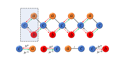
Figure 1: (Color online) Schematic diagram of a non-Hermitian diamond lattice chain consisting of three sites labeled as $(a,b,c)$ per unit cell, enclosed within a black dashed box. Nonreciprocal couplings $Je^{h}$ ($Je^{-h}$) are marked by red (green) solid-line arrows between sublattices $a$ and $c$ in the same unit cell, and sublattices $b$ and $c$ in adjacent unit cells. Synthetic magnetic flux $\theta$ is applied in each closed diamond loop via Peierls’ substitution of the coupling constant between sublattices $b$ and $c$ in the same unit cell.

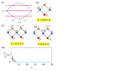
Figure 2: (Color online) Crystalline Case: (a) Energy dispersion $E(k)$ for $\theta=0$ (blue dashed lines) and $\theta=\pi$ (red solid lines). (b)-(d) The CLS occupations of the non-Hermitian diamond lattice in different flat bands for different $\theta$. (e) Density distributions $\rho_{n}^{(l)}$ for six randomly selected eigenstates in dispersive bands with $\theta=0$ under OBCs.

We consider a non-Hermitian diamond chain with quasiperiodic perturbations. In the clean case as schematically illustrated in Fig. 1, there are three sublattices labeled by $a$, $b$, and $c$ in each unit cell. We introduce nonreciprocal couplings marked by solid-line arrows between sublattices $a$ and $c$ in the same unit cell, and sublattices $b$ and $c$ in adjacent unit cells. Moreover, a synthetic magnetic flux $\theta$ is applied in each closed diamond loop via Peierls’ substitution of the coupling constant between sublattices $b$ and $c$ in the same unit cell. Consider the eigenvalue problem of a generalized tight-binding model

$$E\psi_{n}=-J\left[\hat{V}\psi_{n}+\hat{T}_{1}\psi_{n-1}+\hat{T}_{2}\psi_{n+1}\right]+\hat{\epsilon}_{n}\psi_{n},$$ (1)

with

$$\hat{V}=\left(\begin{matrix}0&0&e^{-h}\\ 0&0&e^{-i\theta}\\ e^{h}&e^{i\theta}&0\end{matrix}\right),\hat{T}_{1}=\left(\begin{matrix}0&0&0\\ 0&0&0\\ 1&e^{-h}&0\end{matrix}\right),\hat{T}_{2}=\left(\begin{matrix}0&0&1\\ 0&0&e^{h}\\ 0&0&0\end{matrix}\right),$$ (2)

where each component of the vector $\psi_{n}=(a_{n},b_{n},c_{n})^{T}$ represents a site of a periodic lattice in the $n$-th unit cell, $J$ is the coupling amplitude between adjacent sites with $J=1$ being set as the unit of energy. $h$ is a virtual gauge potential leading to nonreciprocal hoppings and non-Hermitian phenomena in the system. $\theta\in[0,\pi]$ is the synthetic magnetic flux, and the unit cell perturbation $\hat{\epsilon}_{n}$ of the Hamiltonian (1) is given by the diagonal square matrix $\hat{\epsilon}_{n}=\mathrm{diag}(\epsilon_{n}^{a},\epsilon_{n}^{b},\epsilon_{n}^{c})$.

In the crystalline case, where the on-site potential is set to be zero, the clean non-Hermitian model possesses three energy bands under periodic boundary conditions (PBCs) with the dispersion relations given by

$$E_{0}=0,\quad E_{\pm}(k)=\pm 2J\sqrt{1+\cos{\frac{\theta}{2}}\cos(\frac{\theta}{2}+k-ih)},$$ (3)

where $-\pi<k\leq\pi$ is the wave number. For $\theta\neq\pi$, there is only one flat band at energy $E_{0}$, and the other two energy bands are $k$-dependent, which is shown in Fig. 2(a) with $\theta=0$ marked by blue dashed lines. However, for $\theta=\pi$, all of the three bands are dispersionless with the energies $E_{0}=0$ and $E_{\pm}=\pm 2J$ shown in Fig. 2(a) marked by red solid lines. Like the Hermitian case, eigenmodes of our non-Hermitian model corresponding to those $k$-independent energies are CLSs whose amplitudes are nonzero only across a finite number of sites. Figure 2(b) illustrates the fundamental CLS for the $E=0$ state with $\theta=0$ in our cases, which occupies two sites and is localized in a single unit cell. When $\theta\neq 0$ and $E=0$, the fundamental CLSs occupy four sites, shown in Fig. 2(c). The states of the additional flat bands at $E=\pm 2J$ for $\theta=\pi$ host five-site CLSs which excite one of the bottleneck sites seen in Fig. 2(d). Due to the existence of the nonreciprocal hoppings, the states in a dispersive band display the non-Hermitian skin effect under open boundary conditions (OBCs). To display the non-Hermitian skin effect, we calculate the $l$-th eigenstate’s density distribution $\rho_{n}^{(l)}=\sum_{\beta\in\{a,b,c\}}|\psi_{n,\beta}^{(l)}|^{2}$, where $\psi_{n,\beta}^{(l)}$ represents the normalized probability amplitude of the $\beta$ site in the $n$-th unit cell for the $l$-th eigenstate with the number of the unit cell being $N$ and the lattice size being $L=3N$. In Fig. 2(e), we show $\rho_{n}^{(l)}$ for different eigenstates in dispersive bands with $h=0.6$, $\theta=0$, and $N=50$ under OBCs. According to Fig. 2(e), one can see that different states of dispersive bands show the non-Hermitian skin effect.

The effect of quasiperiodic AA perturbations is considered in the present work. The onsite perturbations $\{\epsilon_{n}^{\beta}\}$ for $\beta=\{a,b\}$ are defined as independent AA perturbations

$$\epsilon_{n}^{\beta}=\lambda_{\beta}\cos(2\pi\alpha n+\phi_{\beta}),$$ (4)

where the parameters $\lambda_{\beta}$ are positive real values controlling the quasiperiodic perturbative amplitude, $\phi_{\beta}$ is the phase shift, and $\alpha$ is an irrational number which is set to be the golden ratio $\alpha=(\sqrt{5}-1)/2$. Without loss of generality, we set the $a$-leg phase to be zero ($\phi_{a}=0$). Moreover, the $a$- and $b$-leg perturbation amplitudes are set to be equal to each other $\lambda_{\alpha}=\lambda_{\beta}=\lambda\geq 0$. The $c$-leg potential is a uniform perturbation with the amplitude $\epsilon_{n}^{c}=K\in\mathbb{R}$.

We utilize a local coordinate transformation to the unit cells, which rotates these lattices into a Fano defect form AE2010 ; Flach2014 ; Bodyfelt2014 . The rotation for our non-Hermitian system is defined by a real matrix $\hat{U}$

$$\begin{pmatrix}p_{n}\\ f_{n}\\ c_{n}\\ \end{pmatrix}=\hat{U}\begin{pmatrix}a_{n}\\ b_{n}\\ c_{n}\\ \end{pmatrix},\quad\hat{U}=\frac{1}{\sqrt{2}}\left(\begin{matrix}1&e^{-h}&0\\ e^{h}&-1&0\\ 0&0&\sqrt{2}\end{matrix}\right),$$ (5)

with $\varphi_{n}=(p_{n},f_{n},c_{n})^{T}$ being the rotated tight-binding representation of wave function of the $n$-th unit cell. Lastly, such local coordinate transformation also rotates the onsite perturbation. For the diamond chain, this gives

$$\epsilon_{n}^{\pm}=(\epsilon_{n}^{a}\pm\epsilon_{n}^{b})/2.$$ (6)

From Eq.(6), the remarkable correlations between the $a$- and $b$-leg perturbations appear and will be an object of our studies in this work; namely

$$\begin{aligned} \text{Symmetric:}\quad&\phi_{b}=0&\Leftrightarrow\quad&\epsilon_{n}^{-}=0,\\ \text{Antisymmetric:}\quad&\phi_{b}=\pi&\Leftrightarrow\quad&\epsilon_{n}^{+}=0.\end{aligned}$$ (7)

Since we have set the $a$-leg phase to be zeroed, according to Eq.(6), the correlations can be obtained from the $b$-leg phase, i.e., $\phi_{b}=0$ ($\phi_{b}=\pi$) for the symmetric (antisymmetric) case. In the coming sections, we study how these quasiperiodic modulations at $a$- and $b$-legs and the uniform perturbation at the $c$-leg affect the spectrum and the CLSs.

In the following paper, we utilize the exact diagonalization method to do our numerical calculations. We set $h=0.6$ and $K=0.7$ as a concrete example, and the PBCs are considered.

III Localization features

According to Eq.(5), the diamond lattice’s Eq.(1) become

$$Ep_{n}=\epsilon_{n}^{+}p_{n}+\epsilon_{n}^{-}e^{-h}f_{n}-\frac{1}{\sqrt{2}}(1+e^{-i\theta})e^{-h}c_{n}-\sqrt{2}c_{n+1},$$

$$Ef_{n}=\epsilon_{n}^{+}f_{n}+\epsilon_{n}^{-}e^{h}p_{n}-\frac{1}{\sqrt{2}}(1-e^{-i\theta})c_{n},$$

$$(E-K)c_{n}=-\frac{1}{\sqrt{2}}\left[(1+e^{i\theta})e^{h}p_{n}+(1-e^{i\theta})f_{n}\right]-\sqrt{2}p_{n-1}.$$ (8)

Based on Eq.(8), we discuss different choices of $\theta$ and correlations between the $a$- and $b$-leg perturbations on the system’s localization transitions.

To explore the localization properties of the eigenstates, one can calculate the $l$-th eigenstate’s $q$-dependent fractal dimension Evers2008 ; Ahmed2022 ; Lindinger2019 ; Mac2019 , which is defined as

$$D_{q}^{(l)}=\frac{1}{1-q}\frac{\ln I_{q}^{(l)}}{\ln L}$$ (9)

with the $q$-th order moments being

$$I_{q}^{(l)}=\sum_{n=1}^{N}\sum_{\beta\in\{a,b,c\}}\left|\psi_{n,\beta}^{(l)}\right|^{2q}.$$ (10)

When $q=2$, $I_{2}^{(l)}$ is the known inverse participation ratio (IPR). For a localized state, $I_{2}^{(l)}=O(1)$ in the thermodynamic limit and the corresponding $D_{2}^{(l)}\to 0$, while for an extended state, $I_{2}^{(l)}$ tends to zero in the large system size limit and the corresponding $D_{2}^{(l)}\to 1$. For a multifractal wave function, $D_{2}^{(l)}\in(0,1)$ and the value of $I_{2}^{(l)}$ approaches zero in the $L\to\infty$ limit.

The $q$-dependent fractal dimension $D_{q}^{(l)}$ in the thermodynamic limit can effectively determine the localization features of the system Evers2008 . For a perfectly extended state, $D_{q}^{(l)}\to 1$, where a wave function is distributed throughout the system. For a localized state, the Anderson localization can be observed with the vanishing $D_{q}^{(l)}$ for all $q>0$. $D_{q}^{(l)}\in(0,1)$ corresponds to a multifractal state, which is a feature that the state is delocalized but nonergodic. Furthermore, the multifractal state displays a $q(>0)$ dependence of the fractal dimension $D_{q}^{(l)}$.

To further verify the existence of the multifractal region in our system, we apply the mean inverse participation ratio of a given region $\mathrm{MIPR}(\sigma_{\tilde{\beta}})$ Zeng2017 , which is defined as:

$$\mathrm{MIPR}(\sigma_{\tilde{\beta}})=\frac{1}{\mathcal{N}_{\sigma_{\tilde{\beta}}}}\sum_{l\in\{\sigma_{\tilde{\beta}}\}}I_{2}^{(l)},$$ (11)

Where $\sigma_{\tilde{E}}$, $\sigma_{\tilde{M}}$, and $\sigma_{\tilde{L}}$ represent the spectra localized in the extended, multifractal, and localized regions, respectively, $\tilde{\beta}\in\{\tilde{E},\tilde{M},\tilde{L}\}$, and $\mathcal{N}_{\sigma_{\tilde{\beta}}}$ is the total amount of eigenvalues belonging to $\sigma_{\tilde{\beta}}$. For a finite size system, we use the function $\mathrm{MIPR}(\sigma_{\tilde{\beta}})=\tilde{a}\times(1/L)^{\tilde{b}}+\tilde{c}$ for fitting and obtain the fitting parameters $\tilde{a}$, $\tilde{b}$, and $\tilde{c}$. For a perfectly localized region, $\mathrm{MIPR}(\sigma_{\tilde{L}})$ maintains a constant that hardly changes with $L$. For a perfectly delocalized region, $\mathrm{MIPR}(\sigma_{\tilde{E}})$ varies linearly with $1/L$ and $\tilde{c}\to 0$. When we consider the multifractal region, we can find that the fitting parameter $\tilde{b}\in(0,1)$ with finite $\tilde{a}$, and the fitting parameter $\tilde{c}$ approaches zero Dai2023 .

In addition, many extensions to the AA model have recently been applied to the non-Hermitian systems, where one has systematically examined the relationship between the real-complex transition in energy and the delocalization-localization transition. In a class of AA models with nonreciprocal hoppings under PBCs, one discovered that delocalized states correspond to the complex and localized states to the real energies. Applying such properties, one can also detect the localization transitions of this class of non-Hermitian AA systems with nonreciprocal hoppings Tang2021 .

III.1 The $\theta=0$ cases

We first consider the $\theta=0$ cases, Eq.(8) reads

$$Ep_{n}=\epsilon_{n}^{+}p_{n}+\epsilon_{n}^{-}e^{-h}f_{n}-\sqrt{2}(e^{-h}c_{n}+c_{n+1}),$$

$$Ef_{n}=\epsilon_{n}^{+}f_{n}+\epsilon_{n}^{-}e^{h}p_{n},$$

$$(E-K)c_{n}=-\sqrt{2}(e^{h}p_{n}+p_{n-1}).$$ (12)

We reduce the Eq.(12) to a tight-binding form by expressing the $f_{n}$ and $c_{n}$ variables through the $p_{n}$ ones, which contains the $p_{n}$ variables only:

$$\left(E-\frac{4}{E-K}\right)p_{n}=\tilde{\epsilon}_{n}^{(1)}p_{n}+\frac{2}{E-K}(e^{-h}p_{n-1}+e^{h}p_{n+1}),$$ (13)

where the effective on-site potential

$$\tilde{\epsilon}_{n}^{(1)}=\epsilon_{n}^{+}+\frac{(\epsilon_{n}^{-})^{2}}{E-\epsilon_{n}^{+}}$$ (14)

is a function of the two on-site energies of the diamond lattice $\epsilon_{n}^{a,b}$ in Eq.(4). The effective hopping amplitude depends on the on-site energy $K$ of the $c$-chain.

Notice that regardless of the other system parameters in Eq.(12), it follows that at the energy $E=K$

$$p_{n}=f_{n}=0,\quad c_{n}=e^{h}c_{n+1}.$$ (15)

The state’s amplitudes reside on the $c$ sites. According to Eq.(15), an extended state exists under PBCs and a non-Hermitian skin state under OBCs at the energy $E=K$, independent of the modulation strength $\lambda$. Hence, if the system admits a mobility edge curve, it will diverge $\lambda_{c}(E_{c}=K)=\infty$, yielding a singularity.

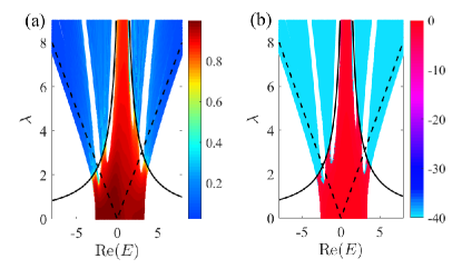
Figure 3: (Color online) Symmetric Case with $\theta=0$: (a) The real part of the spectrum $\sigma_{p,c}$ as a function of $\lambda$, where the color denote the value of the fractal dimension $D_{2}^{(l)}$. (b) $\ln{|\mathrm{Im}(E)|}$ as a function of $\lambda$ and $\mathrm{Re}(E)$. The black solid lines represent the mobility edges given by Eq. (19). The spectrum $\sigma_{f}$ is omitted, but its boundaries are indicated by black dashed lines. Here, $L=600$.

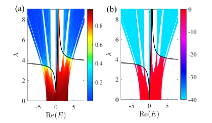
Figure 4: (Color online) Antisymmetric Case with $\theta=0$: (a) The real part of the spectrum as a function of $\lambda$, where the color denote the value of the fractal dimension $D_{2}^{(l)}$. (b) $\ln{|\mathrm{Im}(E)|}$ as a function of $\lambda$ and $\mathrm{Re}(E)$. The black solid lines represent the mobility edges given by Eq. (24). Here, $L=600$.

For the symmetric case $\epsilon_{n}^{-}=0$ obtained by setting $\phi_{b}=0$, Eq.(12) reads

$$Ep_{n}=\epsilon_{n}^{+}p_{n}-\sqrt{2}(e^{-h}c_{n}+c_{n+1}),$$

$$Ef_{n}=\epsilon_{n}^{+}f_{n},$$

$$(E-K)c_{n}=-\sqrt{2}(e^{h}p_{n}+p_{n-1}).$$ (16)

One can see that the $f_{n}$ variables decouple from both the $p_{n}$ and $c_{n}$ variables, producing two independent spectra $\sigma_{f}$ and $\sigma_{p,c}$. The $\sigma_{f}$ keeps its compact feature with the energies given by $E=\epsilon_{n}^{+}$. Hence, all the states belonging to the spectrum $\sigma_{f}$ are localized. In Fig.3, we show the spectrum from Eq.(16) as a function of $\lambda$. Due to the independence of the spectra $\sigma_{f}$ and $\sigma_{p,c}$, we indicate the boundaries of the Fano state spectrum $\sigma_{f}=\{\epsilon_{n}^{+}\}$ by dashed lines in Fig.3, which is equidistributed within the interval $[-\lambda,\lambda]$. To obtain the localization property of $\sigma_{p,c}$, we turn the rotated of Eq.(16) into

$$\tilde{E}^{(1)}p_{n}=\cos(2\pi\alpha n)p_{n}+\frac{2}{\lambda(E-K)}\left(e^{-h}p_{n-1}+e^{h}p_{n+1}\right),$$ (17)

with

$$\tilde{E}^{(1)}=\frac{1}{\lambda}(E-\frac{4}{E-K}).$$ (18)

The dispersive states $p_{n}$ are described by a non-Hermitian AA chain. The nonreciprocal hopping term in Eq.(17) leads to the non-Hermitian behavior of the system and the effective hopping amplitude depends on $\lambda$ and $E$. Referring to the discussion of the localization transition of the non-Hermitian AA model Jiang2019 , we can obtain the mobility edges of the Eq.(17)

$$\left\lvert\frac{2M}{\lambda_{c}(E_{c}-K)}\right\rvert=\frac{1}{2}\quad\Rightarrow\quad\lambda_{c}=\left\lvert\frac{4M}{E_{c}-K}\right\rvert,$$ (19)

with $M=\max\{e^{h},e^{-h}\}$. Figures 3(a) and 3(b) show the fractal dimension $D_{2}^{(l)}$ and the imaginary part of the spectrum $\sigma_{p,c}$ [$\ln{|\mathrm{Im}(E)|}$] of different eigenstates belonging to the spectrum $\sigma_{p,c}$, respectively, as a function of the real part of the corresponding $E$ and the modulation amplitude $\lambda$ with $\theta=0$, $\epsilon_{n}^{-}=0$ and $L=600$ under PBCs. The solid lines in Fig.3 are the analytical solution of mobility edges. The real-complex transition in energy coincides with the localization transition shown in Fig. 3(b). One can see that our analytical result is in excellent agreement with the numerical results.

For the antisymmetric case $\epsilon_{n}^{+}=0$ obtained by $\phi_{b}=\pi$, Eq.(12) transforms into

$$Ep_{n}=\epsilon_{n}^{-}e^{-h}f_{n}-\sqrt{2}(e^{-h}c_{n}+c_{n+1}),$$

$$Ef_{n}=\epsilon_{n}^{-}e^{h}p_{n},$$

$$(E-K)c_{n}=-\sqrt{2}(e^{h}p_{n}+p_{n-1}).$$ (20)

It shows that all flat band states are expelled from their unperturbed energy position $E_{0}$. Since $\epsilon_{n}^{-}\neq 0$, from the second equation of Eq.(20), it follows that at the flat band energy $E_{0}$, we can obtain

$$\epsilon_{n}^{-}e^{h}p_{n}=0\quad\Rightarrow\quad p_{n}=0.$$ (21)

Then, from the first and third equations of Eq.(20), we conclude $f_{n}=c_{n}=0$. Therefore, only the trivial state $(p_{n},f_{n},c_{n})=(0,0,0)$ satisfies Eq.(20) at the flat band energy $E_{0}$. In Figures 4(a) and 4(b), we respectively plot the fractal dimension $D_{2}^{(l)}$ and $\ln{|\mathrm{Im}(E)|}$ as the function of $\mathrm{Re}(E)$ and $\lambda$ in the case of antisymmetry and $\theta=0$ with $L=600$ under PBCs. In this case, mobility edges can be observed. We then derive its analytical forms. For the dispersive part, Eq.(13) reads

$$\tilde{E}^{(2)}p_{n}=\cos(4\pi\alpha n)p_{n}+\frac{4E}{\lambda^{2}(E-K)}\left(e^{-h}p_{n-1}+e^{h}p_{n+1}\right),$$ (22)

with

$$\tilde{E}^{(2)}=\frac{1}{\lambda^{2}}(2E^{2}-\frac{8E}{E-K})-1.$$ (23)

The model becomes a non-Hermitian AA chain eigenequation with the nonreciprocal hoppings and the $\lambda$ and $E$ dependent hopping amplitude. From Ref. Jiang2019 , we can obtain the analytic expression of the mobility edge $\lambda_{c}(E_{c})$:

$$\left\lvert\frac{4E_{c}M}{\lambda_{c}^{2}(E_{c}-K)}\right\rvert=\frac{1}{2}\quad\Rightarrow\quad\lambda_{c}=\sqrt{\left\lvert\frac{8E_{c}M}{E_{c}-K}\right\rvert}.$$ (24)

The analytic curve of the mobility edge Eq.(24) is plotted in Fig.4 marked by the solid lines, displaying agreement with our numerical results.

III.2 The $\theta=\pi$ cases

For the $\theta=\pi$ cases, Eq.(8) becomes

$$Ep_{n}=\epsilon_{n}^{+}p_{n}+\epsilon_{n}^{-}e^{-h}f_{n}-\sqrt{2}c_{n+1},$$

$$Ef_{n}=\epsilon_{n}^{+}f_{n}+\epsilon_{n}^{-}e^{h}p_{n}-\sqrt{2}c_{n},$$

$$(E-K)c_{n}=-\sqrt{2}(f_{n}+p_{n-1}).$$ (25)

We reduce the Eq.(25) to a tight-binding form by expressing the $f_{n}$ and $c_{n}$ variables through the $p_{n}$ ones, which contains the $p_{n}$ variables only:

$$\left(E-\frac{2}{E-K}\right)p_{n}= \tilde{\epsilon}_{n}^{(2)}p_{n}+\frac{2}{E-K}(\tilde{J}_{n}e^{-h}p_{n-1}$$

$$+\tilde{J}_{n+1}e^{h}p_{n+1}),$$ (26)

where the effective on-site perturbation amplitude

$$\tilde{\epsilon}_{n}^{(2)}=\epsilon_{n}^{+}+\frac{(\epsilon_{n}^{-})^{2}}{E-\epsilon_{n}^{+}-\frac{2}{E-K}}+\frac{(\frac{2}{E-K})^{2}}{E-\epsilon_{n+1}^{+}-\frac{2}{E-K}},\\$$ (27)

and

$$\tilde{J}_{n}=\frac{\epsilon_{n}^{-}}{E-\epsilon_{n}^{+}-\frac{2}{E-K}}.$$ (28)

The reduced topology displays a complex tight-binding form with the on-site perturbation term and the hopping terms being $\epsilon_{n}^{+}$, $\epsilon_{n}^{-}$, and $K$ dependent, which should present complex localization properties.

When we consider the symmetric case $\epsilon_{n}^{-}=0$, according to Eq.(25), the intracell and intercell information can be written as the matrix form:

$$\hat{V}^{(1)}=\left(\begin{matrix}0&0&0\\ 0&0&\sqrt{2}\\ 0&\sqrt{2}&0\end{matrix}\right),\quad\hat{T}^{(1)}=\left(\begin{matrix}0&0&0\\ 0&0&0\\ \sqrt{2}&0&0\end{matrix}\right).$$ (29)

And the lattice eigenvalue equation similar to Eq. (1) reads

$$E\varphi_{n}=-\left[\hat{V}^{(1)}\varphi_{n}+\hat{T}^{(1)}\varphi_{n-1}+\hat{T}^{(1)\dagger}\varphi_{n+1}\right]+\hat{\epsilon}_{n}^{(1)}\varphi_{n},$$ (30)

with the on-site disorder matrix $\hat{\epsilon}_{n}^{(1)}=\mathrm{diag}(\epsilon_{n}^{+},\epsilon_{n}^{+},K)$. A new unit cell can be identified considering the connected lattice sites $\tilde{\varphi}_{n}=(p_{n-1},f_{n},c_{n})$, which affirms that the CLS of the disorder-free limit stays in one unit cell. The corresponding information on the intracell and the intercell reads

$$\hat{V}^{(2)}=\left(\begin{matrix}0&0&\sqrt{2}\\ 0&0&\sqrt{2}\\ \sqrt{2}&\sqrt{2}&0\end{matrix}\right),\quad\hat{T}^{(2)}=\left(\begin{matrix}0&0&0\\ 0&0&0\\ 0&0&0\end{matrix}\right),$$ (31)

with the lattice eigenvalue equation

$$E\tilde{\varphi}_{n}=-\left[\hat{V}^{(2)}\tilde{\varphi}_{n}+\hat{T}^{(2)}\tilde{\varphi}_{n-1}+\hat{T}^{(2)\dagger}\tilde{\varphi}_{n+1}\right]+\hat{\epsilon}_{n}^{(2)}\tilde{\varphi}_{n},$$ (32)

where $\hat{\epsilon}_{n}^{(2)}=\mathrm{diag}(\epsilon_{n-1}^{+},\epsilon_{n}^{+},K)$. Observing the geometric information above, one can find that Eq.(32) displays the vanishing of the hopping between adjacent unit cells and the hopping term only exists within one unit cell. The extensive degeneracy is broken with the energy being modulation-dependent. With the help of the transformation, we display that the symmetric case with $\theta=\pi$ is made of three-site unit cells but with the absence of intercell hoppings, indicating the preservation of the CLSs even in the presence of the disorder. It means that all the states in such case are localized.

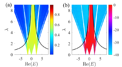
Figure 5: (Color online) Antisymmetric Case with $\theta=\pi$: (a) The real part of the spectrum as a function of $\lambda$, where the color denote the value of the fractal dimension $D_{2}^{(l)}$. (b) $\ln{|\mathrm{Im}(E)|}$ as a function of $\lambda$ and $\mathrm{Re}(E)$. The black solid lines represent the multifractal-to-localized edges given by Eq. (36). Here, $L=600$.

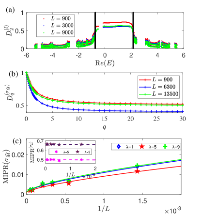
Figure 6: (Color online) Antisymmetric Case with $\theta=\pi$: (a) $D_{2}^{(l)}$ for each eigenstate at different system sizes with $\lambda=5$. (b) The $q$-dependent fractal dimension $D_{q}^{(\sigma_{\tilde{M}})}$ by averaging over all the eigenstates localized in the region between two multifractal-to-localized edges vs $q$ for various system sizes with $\lambda=5$. (c) The scaling of $\mathrm{MIPR}(\sigma_{\tilde{M}})$ for different $\lambda$. The inset shows the scaling of $\mathrm{MIPR}(\sigma_{\tilde{L}})$ for different $\lambda$.

For the antisymmetric case $\epsilon_{n}^{+}=0$, Eq.(25) reads

$$Ep_{n}=e^{-h}\epsilon_{n}^{-}f_{n}-\sqrt{2}c_{n+1},$$

$$Ef_{n}=e^{h}\epsilon_{n}^{-}p_{n}-\sqrt{2}c_{n},$$

$$(E-K)c_{n}=-\sqrt{2}(f_{n}+p_{n-1}).$$ (33)

For the $E=K$ case, one can obtain the equation of the tight-binding form by substituting $f_{n}$ and $c_{n}$ variables:

$$-2Kp_{n}=\lambda\left[\cos(2\pi n\alpha)e^{-h}p_{n-1}+\cos(2\pi(n+1)\alpha)e^{h}p_{n+1}\right].$$ (34)

This model is equivalent to the non-Hermitian off-diagonal Harper model Tang2021 , where the $E=K$ modes remain multifractal for all the modulation amplitude.

For the $E\neq K$ case, substituting the $f_{n}$, $c_{n}$ variables by the $p_{n}$ ones, we can obtain the following equation:

$$\tilde{E}^{(2)}p_{n}= \cos(4\pi\alpha n)p_{n}+\frac{4}{\lambda(E-K)}\big{\{}\cos(2\pi\alpha n)e^{-h}p_{n-1}$$

$$+\cos[2\pi\alpha(n+1)]e^{h}p_{n+1}\big{\}}.$$ (35)

This equation is similar to a generalized Harper model with nonreciprocal hoppings Tang2021 , but its on-site perturbation frequency is twice that of the hoppings. According to Refs. Dombrowski1978 ; Marx2017 , it has not been allowed extended states that the mode described by Eq.(35). We plot the fractal dimension $D_{2}^{(l)}$ and $\ln{|\mathrm{Im}(E)|}$ as the function of $\mathrm{Re}(E)$ and $\lambda$ in the case of antisymmetry and $\theta=\pi$ with $L=600$ under PBCs, shown in Figs. 5(a) and 5(b), respectively. According to the numerical calculation, we can obtain the delocalized-to-localized edges

$$\lambda_{c}=\left\lvert\frac{4M}{E_{c}-K}\right\rvert,$$ (36)

which are plotted in Fig.5 marked by the solid lines. In the Hermitian limit with $h=0$, Eq.(36) reduces to $\lambda_{c}=4/|E_{c}-K|$, which has been studied numerically in Ref. Ahmed2022 . One can see that in Fig. 5(a), the values of $D_{2}^{(l)}$ localized in the internal region between the two solid lines are around $0.55$ to $0.7$, indicating that the states in this region may be multifractal under PBCs.

To further determine the localization properties in this case, we consider the fractal dimensions $D_{2}^{(l)}$ for each eigenstate at different system sizes, which is shown in Fig. 6(a) with $\lambda=5$ and $\theta=\pi$ under PBCs. In the finite-size case, the fractal dimensions of the states in the localized regions extrapolate to $0$. In contrast, the fractal dimension’s values of the internal region between two analytical edges shown by Eq.(36) with $\lambda=5$ are away from $0$ and $1$ for different sizes, which implies that the states in this internal region are multifractal, and the analytical edges correspond to the multifractal-to-localized edges. We also calculate the $q$-dependent fractal dimensions $D_{q}^{(\sigma_{\tilde{M}})}$ by averaging over all the eigenstates localized in the region between two multifractal-to-localized edges as shown in Fig. 6(b) with $\lambda=5$ and $\theta=\pi$ under PBCs. We can see that for all $q>0$, $D_{q}^{(\sigma_{\tilde{M}})}\in(0,1)$ displays a nontrivial dependence on the moment $q$. This indicates that the states in the internal region exhibit multifractal behavior. Furthermore, we calculate $\mathrm{MIPR}(\sigma_{\tilde{M}})$ as a function of $1/L$ for different $L$ with $\theta=\pi$, which is shown in Fig.6(c). When $\lambda=1$, all the states are multifractal, and the corresponding fitting parameters of $\mathrm{MIPR}(\sigma_{\tilde{M}})$ are $\tilde{a}\approx 1.27$, $\tilde{b}\approx 0.705$, and $\tilde{c}\to 0$, respectively. For the $\lambda=5$ case, the mulitfractal-to-localized edges are at $E_{c1}\approx-0.75$ and $E_{c2}\approx 2.15$, and the corresponding fitting function is $\mathrm{MIPR}_{\lambda=5}(\sigma_{\tilde{M}})\approx 1.018L^{-0.699}$ with $\tilde{c}\to 0$. The mulitfractal-to-localized edges of $\lambda=9$ are at $E_{c1}\approx-0.1$ and $E_{c2}\approx 1.5$. The fitting function is $\mathrm{MIPR}_{\lambda=9}(\sigma_{\tilde{M}})\approx 1.061L^{-0.670}$ with $\tilde{c}\to 0$. According to the fitting parameters of the mean inverse participation ratios of the internal regions, we can further determine that the states in the internal regions are multifractal. We also show the scaling of $\mathrm{MIPR}(\sigma_{\tilde{L}})$ for $\lambda=5$ and $9$ in the inset of Fig. 6(c). Both cases display the $L$-independent behavior, and in the thermodynamic limit, $\mathrm{MIPR}(\sigma_{\tilde{L}})$ tend to finite values. Our results imply that the system has multifractal-to-localized edges for the $\theta=\pi$ and antisymmetric case, which can separate the multifractal states from the localized ones.

III.3 The $\theta\in(0,\pi)$ cases

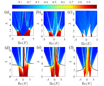
Figure 7: (Color online) $D_{2}^{(l)}$ as a function of $\lambda$ and $\mathrm{Re}(E)$ with $L=600$. The top row corresponds to the symmetric cases, and the bottom row corresponds to the antisymmetric cases. From the left column to the right column, $\theta=0.15\pi$, $0.5\pi$, and $0.9\pi$, respectively.

According to the above discussions, the system displays distinct localization features for the $\theta=0$ and $\theta=\pi$ cases. In this subsection, we consider when $\theta\in(0,\pi)$, the localization properties for both symmetric and antisymmetric cases.

For $\theta\in(0,\pi)$ and the symmetric case $\epsilon_{n}^{-}=0$, Eq. (8) reads

$$Ep_{n}=\epsilon_{n}^{+}p_{n}-\frac{1}{\sqrt{2}}(1+e^{-i\theta})e^{-h}c_{n}-\sqrt{2}c_{n+1},$$

$$Ef_{n}=\epsilon_{n}^{+}f_{n}-\frac{1}{\sqrt{2}}(1-e^{-i\theta})c_{n},$$

$$(E-K)c_{n}=-\frac{1}{\sqrt{2}}\left[(1+e^{i\theta})e^{h}p_{n}+(1-e^{i\theta})f_{n}\right]-\sqrt{2}p_{n-1}.$$ (37)

When $\theta=0$, according to Eq.(16), we can see that the system presents two independent spectra, $\sigma_{f}$ and $\sigma_{p,c}$, where the $\sigma_{f}$ keeps the localized properties and the $\sigma_{p,c}$ displays the mobility edges separating the extended states from the localized ones. Figures 7(a)-7(c) show the fractal dimension $D_{2}^{(l)}$ of different eigenstates as a function of $\mathrm{Re}(E)$ and the modulation amplitude $\lambda$ for $\epsilon_{n}^{-}=0$ with $\theta=0.15\pi$, $0.5\pi$, and $0.9\pi$, respectively. In the small $\theta$ case, the spectra $\sigma_{f}$ and $\sigma_{p,c}$ begin to couple together and display a weak coupling at the edges of the two spectra. With the increase of $\theta$, in the small $\lambda$ case, the proportion of the extended states gradually decreases in the band-edge regions. However, the band-center region gradually changes from a mixture regime with both extended and localized states to a multifractal regime to a localized regime. When $\theta\to\pi$, all the states become localized for an arbitrary finite $\lambda$. According to our numerical calculation, we can see that, in this case, the system displays a complex localization feature, and the existence of extended, localized, and multifractal regimes is detected.

For the antisymmetric case $\epsilon_{n}^{+}=0$, Eq.(8) reads

$$Ep_{n}=\epsilon_{n}^{-}e^{-h}f_{n}-\frac{1}{\sqrt{2}}(1+e^{-i\theta})e^{-h}c_{n}-\sqrt{2}c_{n+1},$$

$$Ef_{n}=\epsilon_{n}^{-}e^{h}p_{n}-\frac{1}{\sqrt{2}}(1-e^{-i\theta})c_{n},$$

$$(E-K)c_{n}=-\frac{1}{\sqrt{2}}\left[(1+e^{i\theta})e^{h}p_{n}+(1-e^{i\theta})f_{n}\right]-\sqrt{2}p_{n-1}.$$ (38)

We can obtain the exact extended-to-localized edges at $\theta=0$, and when $\theta=\pi$, the multifractal-to-localized edges are given by Eq.(36). To obtain the localization information for an arbitrary $\theta$, we plot $D_{2}^{(l)}$ as a function of $\mathrm{Re}(E)$ and the modulation amplitude $\lambda$ for $\epsilon_{n}^{+}=0$ with $\theta=0.15\pi$, $0.5\pi$, and $0.9\pi$ shown in Figs. 7(d)-7(f), respectively. We find that the delocalization-to-localization transition can be described by the equation

$$\lambda_{c}=2\sqrt{\Big{|}\frac{E_{c}M}{E_{c}-K}\Big{|}\sqrt{2(1+\cos\theta)}+\frac{2(1-\cos\theta)M^{2}}{(E_{c}-K)^{2}}},$$ (39)

which is plotted as the black solid lines in Figs. 7(d)-7(f). Despite the lack of analytical proof, the relation Eq.(39) works well in separating the delocalized and localized regimes, in this case, with different $\theta$. Eq.(39) can be considered an empirical combination of the corresponding analytical results under different limitations. When $\theta\to 0$, Eq.(39) reduces to Eq.(24), and for $\theta\to\pi$, Eq.(39) reduces to Eq.(36). Our results also suit the Hermitian cases with $h=0$. Moreover, as seen in Figs.7(d)-7(e), the multifractal states are induced by increasing $\theta$, and for an intermediate $\theta$, it displays an extended and multifractal mixture in the band-center region.

IV Conclusion

This paper investigates the effects of a quasiperiodic AA perturbation on a one-dimensional non-Hermitian diamond lattice featuring flat bands. In the crystalline limit, only one flat band at $E_{0}=0$ for $\theta\neq\pi$, while the other two bands exhibit a dependence on the wave vector $k$. However, for $\theta=\pi$, the non-Hermitian diamond lattice presents three dispersionless bands with energies $E_{0}=0$ and $E_{\pm}=\pm 2J$. We observe that the fate of the CLSs depends on the symmetry of the applied perturbation and the choice of the synthetic magnetic flux $\theta$. We examine the consequences of applying the perturbation in two distinct ways: symmetric and antisymmetric. In the $\theta=0$ cases, we find that the symmetric perturbation leads to the decoupling of the $f_{n}$ variables from the $p_{n}$ and $c_{n}$ ones, yielding two independent spectra $\sigma_{f}$ and $\sigma_{p,c}$. The $\sigma_{f}$ retains its compact characteristics, while the $\sigma_{p,c}$ exhibits analytical mobility edges as described in Eq.(19). In the antisymmetric case, the energies of CLSs are expelled from $E_{0}$. Furthermore, the dispersive part manifests exact mobility edges as expressed in Eq.(24). In the $\theta=\pi$ cases, when considering the diagonal perturbation symmetrically, all the eigenstates remain compactly localized, although the extensive degeneracy is disrupted. However, for antisymmetric perturbation, the degeneracy is broken, and the eigenstates no longer remain compactly localized. An exploration of the nature of the eigenstates using various observables reveals the emergence of the flat band based multifractal states. We determine the multifractal-to-localized edges using the numerical tools, as outlined in Eq.(36) . Finally, in the $\theta\in(0,\pi)$ cases, when studying the effect of the symmetric perturbation, localization features exhibit a complex evolution as $\theta$ increases from $0$ to $\pi$. In the antisymmetric case, we propose an expression for the delocalization-to-localization transition, which aligns well with our numerical findings.

- (1) P. W. Anderson, Phys. Rev. 109, 1492 (1958).
- (2) P. A. Lee and T. V. Ramakrishnan, Rev. Mod. Phys. 57, 287 (1985).
- (3) D. S. Wiersma, P. Bartolini, A. Lagendijk, and R. Righini, Nature (London) 390, 671 (1997).
- (4) J. Topolancik, B. Ilic, and F. Vollmer, Phys. Rev. Lett. 99, 253901 (2007).
- (5) T. Schwartz, G. Bartal, S. Fishman, and M. Segev, Nature (London) 446, 52 (2007).
- (6) M. Lopez, J.-F. Clément, P. Szriftgiser, J. C. Garreau, and D. Delande, Phys. Rev. Lett. 108, 095701 (2012).
- (7) I. Manai, J.-F. Clément, R. Chicireanu, C. Hainaut, J. C. Garreau, P. Szriftgiser, and D. Delande, Phys. Rev. Lett. 115, 240603 (2015).
- (8) R. S. Whitney, Phys. Rev. Lett. 112, 130601 (2014).
- (9) J. Billy, V. Josse, Z. Zuo, A. Bernard, B. Hambrecht, P. Lugan, D. Clément, L. Sanchez-Palencia, P. Bouyer, and A. Aspect, Nature (London) 453, 891 (2008).
- (10) G. Roati, C. D’Errico, L. Fallani, M. Fattori, C. Fort, M. Zaccanti, G. Modugno, M. Modugno, and M. Inguscio, Nature (London) 453, 895 (2008).
- (11) S. S. Kondov, W. R. McGehee, J. J. Zirbel, and B. DeMarco, Science 334, 66 (2011).
- (12) F. Jendrzejewski, A. Bernard, K. Müller, P. Cheinet, V. Josse, M. Piraud, L. Pezzé, L. Sanchez-Palencia, A. Aspect, and P. Bouyer, Nat. Phys. 8, 398 (2012).
- (13) G. Semeghini, M. Landini, P. Castilho, S. Roy, G. Spagnolli, A. Trenkwalder, M. Fattori, M. Inguscio, and G. Modugno, Nat. Phys. 11, 554 (2015).
- (14) M. Pasek, G. Orso, and D. Delande, Phys. Rev. Lett. 118, 170403 (2017).
- (15) H. Hu, A. Strybulevych, J. H. Page, S. E. Skipetrov, and B. A. van Tiggelen, Nat. Phys. 4, 945 (2008).
- (16) A. A. Chabanov, M. Stoytchev, and A. Z. Genack, Nature (London) 404, 850 (2000).
- (17) P. Pradhan and S. Sridhar, Phys. Rev. Lett. 85, 2360 (2000).
- (18) N. Mott, J. Phys. C 20, 3075 (1987).
- (19) I. F. Herrera-González and J. A. Méndez-Bermúdez, Phys. Rev. E 107, 034108 (2023).
- (20) Y. Wang, L. Zhang, W. Sun, T.-F. J. Poon, and X.-J. Liu, Phys. Rev. B 106, L140203 (2022).
- (21) C. Chiaracane, M. T. Mitchison, A. Purkayastha, G. Haack, and J. Goold, Phys. Rev. Res. 2, 013093 (2020).
- (22) K. Yamamoto, A. Aharony, O. Entin-Wohlman, and N. Hatano, Phys. Rev. B 96, 155201 (2017).
- (23) L. Zhou, Phys. Rev. B 108, 014202 (2023).
- (24) Y. Wang, J.-H. Zhang, Y. Li, J. Wu, W. Liu, F. Mei, Y. Hu, L. Xiao, J. Ma, C. Chin, and S. Jia, Phys. Rev. Lett. 129, 103401 (2022).
- (25) S. Aubry and G. André, Ann. Isr. Phys. Soc. 3, 133 (1980).
- (26) Y. Lahini, R. Pugatch, F. Pozzi, M. Sorel, R. Morandotti, N. Davidson, and Y. Silberberg, Phys. Rev. Lett. 103, 013901 (2009).
- (27) S. Longhi, Phys. Rev. Lett. 122, 237601 (2019).
- (28) S. Longhi, Phys. Rev. B 100, 125157 (2019).
- (29) J. Biddle and S. Das Sarma. Phys. Rev. Lett. 104, 070601 (2010).
- (30) Y. Liu, X.-P. Jiang, J. Cao, and S. Chen, Phys. Rev. B 101, 174205 (2020).
- (31) Y. Wang, X. Xia, L. Zhang, H. Yao, S. Chen, J. You, Q. Zhou, and X.-J. Liu, Phys. Rev. Lett. 125, 196604 (2020).
- (32) T. Liu, H. Guo, Y. Pu, and S. Longhi, Phys. Rev. B 102, 024205 (2020).
- (33) Z. Xu, X. Xia, and S. Chen, Sci. China: Phys. Mech. Astron. 65, 227211 (2022).
- (34) S. Ganeshan, J. H. Pixley, and S. D. Sarma, Phys. Rev. Lett. 114, 146601 (2015).
- (35) X. Li and S. Das Sarma, Phys. Rev. B 96, 085119 (2017).
- (36) X. Deng, S. Ray, S. Sinha, G. V. Shlyapnikov, and L. Santos, Phys. Rev. Lett. 123, 025301 (2019).
- (37) Z. Xu, H. Huangfu, Y. Zhang, and S. Chen, New J. Phys. 22, 013036 (2020).
- (38) Q. Dai, Z. Lu, and Z. Xu, Phys. Rev. B 108, 144207 (2023).
- (39) T. Liu, X. Xia, S. Longhi, and L. Sanchez-Palencia, SciPost Phys. 12, 027 (2022).
- (40) M. Maksymenko, A. Honecker, R. Moessner, J. Richter, and O. Derzhko, Phys. Rev. Lett. 109, 096404 (2012).
- (41) D. Leykam, A. Andreanov, and S. Flach, Adv. Phys.: X 3, 1473052 (2018).
- (42) J.-W. Rhim and B.-J. Yang, Adv. Phys.: X 6, 1901606 (2021).
- (43) S. Talkington and M. Claassen, Phys. Rev. B 106, L161109 (2022).
- (44) C. V. Morfonios, M. Röntgen, M. Pyzh, and P. Schmelcher, Phys. Rev. B 104, 035105 (2021).
- (45) Y. Kuno, T. Mizoguchi, and Y. Hatsugai, Phys. Rev. B 102, 241115(R) (2020).
- (46) D. Leykam, S. Flach, O. Bahat-Treidel, and A. S. Desyatnikov, Phys. Rev. B 88, 224203 (2013).
- (47) B. Pal and K. Saha, Phys. Rev. B 97, 195101 (2018).
- (48) W. Zhang, Z. Addison, and N. Trivedi, Phys. Rev. B 104, 235202 (2021).
- (49) H. Ramezani, Phys. Rev. A 96, 011802(R) (2017).
- (50) M. Hyrkäs, V. Apaja, and M. Manninen, Phys. Rev A 87, 023614 (2013).
- (51) O. Derzhko, J. Richter, A. Honecker, M. Maksymenko, and R. Moessner, Phys. Rev. B 81, 014421 (2010).
- (52) M. Goda, S. Nishino, and H. Matsuda, Phys. Rev. Lett. 96, 126401 (2006).
- (53) S. D. Huber and E. Altman, Phys. Rev. B 82, 184502 (2010).
- (54) D. Green, L. Santos, and C. Chamon, Phys. Rev. B 82, 075104 (2010).
- (55) B. Sutherland, Phys. Rev. B 34, 5208 (1986).
- (56) H. Aoki, M. Ando, and H. Matsumura, Phys. Rev. B 54, R17296(R) (1996).
- (57) D. Leykam, J. D. Bodyfelt, A. S. Desyatnikov, and S. Flach, Eur. Phy. J. B 90, 1 (2017).
- (58) C. Gneiting, Z. Li, and F. Nori, Phys. Rev. B 98, 134203 (2018).
- (59) M. Tovmasyan, S. Peotta, L. Liang, P. Törmä, and S. D. Huber, Phys. Rev. B 98, 134513 (2018).
- (60) J. Vidal, B. Douçot, R. Mosseri, and P. Butaud, Phys. Rev. Lett. 85, 3906 (2000).
- (61) S. Mukherjee, M. Di Liberto, P. Öhberg, R. R. Thomson, and N. Goldman, Phys. Rev. Lett. 121, 075502 (2018).
- (62) G.-W. Chern, C.-C. Chien, and M. Di Ventra, Phys. Rev. A 90, 013609 (2014).
- (63) A. R. Kolovsky, A. Ramachandran, and S. Flach, Phys. Rev. B 97, 045120 (2018).
- (64) T. Mizoguchi and M. Udagawa, Phys. Rev. B 99, 235118 (2019).
- (65) H. Tian, X. Gao, Y. Zhang, S. Che, T. Xu, P. Cheung, K. Watanabe, T. Taniguchi, M. Randeria, F. Zhang, C. N. Lau, and M. W. Bockrath, Nature (London) 614, 440 (2023).
- (66) H. Tasaki, Phys. Rev. Lett. 69, 1608 (1992).
- (67) S. Peotta and P. Törmä, Nat. Commun. 6, 8944 (2015).
- (68) S. Longhi, Opt. Lett. 46, 2872 (2021).
- (69) H. Wang, W. Zhang, H. Sun, and X. Zhang, Phys. Rev. B 106, 104203 (2022).
- (70) H. Li, Z. Dong, S. Longhi, Q. Liang, D. Xie, and B. Yan, Phys. Rev. Lett. 129, 220403 (2022).
- (71) W. Zhang, H. Wang, H. Sun, and X. Zhang, Phys. Rev. Lett. 130, 206401 (2023).
- (72) J. D. Bodyfelt, D. Leykam, C. Danieli, X. Yu, and S. Flach, Phys. Rev. Lett. 113, 236403 (2014).
- (73) C. Danieli, J. D. Bodyfelt, and S. Flach, Phys. Rev. B 91, 235134 (2015).
- (74) A. Ahmed, A. Ramachandran, I. M. Khaymovich, and A.Sharma, Phys. Rev. B 106, 205119 (2022).
- (75) S. Lee, A. Andreanov, and S. Flach, Phys. Rev. B 107, 014204 (2023).
- (76) S. Lee, S. Flach, and A. Andreanov, Chaos 33, 073125 (2023).
- (77) C. Liu, H. Jiang, and S. Chen, Phys. Rev. B 99, 125103 (2019).
- (78) C. Liu, and S. Chen, Phys. Rev. B 100, 144106 (2019).
- (79) H. Shen, B. Zhen, and L. Fu, Phys. Rev. Lett. 120, 146402 (2018).
- (80) H. Schomerus, Phys. Rev. Res. 2, 013058 (2020).
- (81) C. M. Bender and S. Boettcher, Phys. Rev. Lett. 80, 5243(1998).
- (82) H. Zhao, P. Miao, M. H. Teimourpour, S. Malzard, R. ElGanainy, H. Schomerus, and L. Feng, Nat. Commun. 9, 981 (2018).
- (83) C. Poli, M. Bellec, U. Kuhl, F. Mortessagne, and H. Schomerus, Nat. Commun. 6, 6710 (2015).
- (84) S. Malzard, C. Poli, and H. Schomerus, Phys. Rev. Lett. 115, 200402 (2015).
- (85) H. Ghaemi-Dizicheh and H. Schomerus, Phys. Rev. A 104, 023515 (2021).
- (86) H. Zhou, C. Peng, Y. Yoon, C. W. Hsu, K. A. Nelson, L. Fu, J. D. Joannopoulos, M. Soljacic, and B. Zhen, Science 359, 1009 (2018).
- (87) K. Zhang, C. Fang, and Z. Yang, Phys. Rev. Lett. 131, 036402 (2023).
- (88) H. Jiang and C. H. Lee, Phys. Rev. Lett. 131, 076401 (2023).
- (89) H. Wetter, M. Fleischhauer, S. Linden, and J. Schmitt, Phys. Rev. Lett. 131, 083801 (2023).
- (90) Q. Zhang, Y. Li, H. Sun, X. Liu, L. Zhao, X. Feng, X. Fan, and C. Qiu, Phys. Rev. Lett. 130, 017201 (2023).
- (91) G. Chen, F. Song, and J. L. Lado, Phys. Rev. Lett. 130, 100401 (2023).
- (92) L. Jezequel and P. Delplace, Phys. Rev. Lett. 130, 066601 (2023).
- (93) Q. Wang, C. Zhu, X. Zheng, H. Xue, B. Zhang, and Y. D. Chong, Phys. Rev. Lett. 130, 103602 (2023).
- (94) R. Shen, Y. Guo, and S. Yang, Phys. Rev. Lett. 130, 220401 (2023).
- (95) G. Xu, X. Zhou, Y. Li, Q. Cao, W. Chen, Y. Xiao, L. Yang, and C.-W. Qiu, Phys. Rev. Lett. 130, 266303 (2023).
- (96) H. Jiang, L.-J. Lang, C. Yang, S.-L. Zhu, and S. Chen, Phys. Rev. B 100, 054301 (2019).
- (97) S. Yao, F. Song, and Z. Wang, Phys. Rev. Lett. 121, 136802 (2018).
- (98) S. Yao and Z. Wang, Phys. Rev. Lett. 121, 086803 (2018).
- (99) Z. Gong, Y. Ashida, K. Kawabata, K. Takasan, S. Higashikawa, and M. Ueda, Phys. Rev. X 8, 031079 (2018).
- (100) Z. Xu, X. Xia, and S. Chen, Phys. Rev. B 104, 224204 (2021).
- (101) N. Hatano and D. R. Nelson, Phys. Rev. Lett. 77, 570 (1996).
- (102) N. Hatano and D. R. Nelson, Phys. Rev. B 56, 8651 (1997).
- (103) N. Hatano and D. R. Nelson, Phys. Rev. B 58, 8384 (1998).
- (104) A. E. Miroshnichenko, S. Flach, and Y. S. Kivshar, Rev. Mod. Phys. 82, 2257 (2010).
- (105) S. Flach, D. Leykam, J. D. Bodyfelt, P. Matthies, and A. S. Desyatnikov, Europhys. Lett. 105, 30001 (2014).
- (106) F. Evers and A. D. Mirlin, Rev. Mod. Phys. 80, 1355 (2008).
- (107) J. Lindinger, A. Buchleitner, and A. Rodríguez, Phys. Rev. Lett. 122, 106603 (2019).
- (108) N. Macé, F. Alet, and N. Laflorencie, Phys. Rev. Lett. 123, 180601 (2019).
- (109) Qi-B. Zeng, S. Chen, and R. Lü, Phys. Rev. A 95, 062118 (2017).
- (110) L.-Z. Tang, G.-Q. Zhang, L.-F. Zhang, and D.-W. Zhang, Phys. Rev. A 103, 033325 (2021).
- (111) J. Dombrowski, Proc. Amer. Math. Soc. 69, 95 (1978).
- (112) C. A. Marx and S. Jitomirskaya, Ergod. Th. Dynam. Sys. 37, 2353 (2017).