TabRepo: A Large Scale Repository of Tabular Model Evaluations and its AutoML Applications

Abstract

We introduce TabRepo, a new dataset of tabular model evaluations and predictions. TabRepo contains the predictions and metrics of 1206 models evaluated on 200 classification and regression datasets. We illustrate the benefit of our dataset in multiple ways. First, we show that it allows to perform analysis such as comparing Hyperparameter Optimization against current AutoML systems while also considering ensembling at no cost by using precomputed model predictions. Second, we show that our dataset can be readily leveraged to perform transfer-learning. In particular, we show that applying standard transfer-learning techniques allows to outperform current state-of-the-art tabular systems in accuracy, runtime and latency.

1 Introduction

Machine learning on structured tabular data has a long history due to its wide range of practical applications. Significant progress has been achieved through improving supervised learning models, with key method landmarks including SVM (Hearst et al., 1998), Random Forest (Breiman, 2001) and Gradient Boosted Trees (Friedman, 2001). While the performance of base models is still being improved by a steady stream of research, their performance has saturated and state-of-the-art methods now leverage AutoML techniques (He et al., 2021) or new paradigms such as the pretraining of transformer models (Hollmann et al., 2022).

AutoML solutions currently dominate tabular prediction benchmarks (Erickson et al., 2020; Gijsbers et al., 2022). Auto-Sklearn (Feurer et al., 2015a; 2020) was an early approach that proposed to select pipelines to ensemble from the Sklearn library and meta-learn the hyperparameter-optimization (HPO) with offline evaluations. The approach was successful and won several AutoML competitions. Several frameworks followed with other AutoML approaches such as TPOT (Olson & Moore, 2016), H2O AutoML (LeDell & Poirier, 2020), and AutoGluon (Erickson et al., 2020). AutoGluon particularly showed strong performance by combining ensembling (Caruana et al., 2004), stacking (Wolpert, 1992) and bagging (Breiman, 1996). While all techniques were shown to be important to reach good accuracy, they also bear a significant cost in terms of training time as models are fitted on several folds of the training data and the stacking of models strongly impacts inference latency.

The proliferation of AutoML and supervised learning methods led to several works focusing on benchmarking tabular methods. Recently, Gijsbers et al. (2022) proposed a unified benchmark called the AutoMLBenchmark to compare tabular methods. However, the cost of running such comparisons for new methods becomes quickly prohibitive. Evaluating a single method in the AutoMLBenchmark requires 40000 CPU hours of compute . This limits the number of methods present in the benchmark and restricts research and experimentation to those with access to sufficient computational resources. For instance, measuring the impact of ensembling requires retraining the base models which can easily become too expensive in particular given many datasets and seeds.

To address this issue, we introduce TabRepo, a dataset of model evaluations and predictions. The main contributions of this paper are:

• A large scale evaluation of tabular models comprising 723600 model predictions with 1206 models from 6 different families which are evaluated across 200 datasets and 3 seeds.

• We show how the repository can be used to study at no cost the performance of tuning models while considering ensembles by leveraging precomputed model predictions.

• We show that our dataset combined with transfer learning achieves a result competitive with state-of-the-art AutoML systems and outperforms others by a significant amount in accuracy and training time.

• We study the performance of transfer learning techniques on tabular methods across several novel angles such as data efficiency, training time, and prediction latency.

This paper first reviews related work before describing the TabRepo dataset. We then illustrate how TabRepo can be leveraged to compare HPO with ensemble against current state-of-the-art tabular systems and finally show how transfer-learning can be used to outperform current systems.

2 Related work

Acquiring and re-using offline evaluations to eliminate redundant computation has been proposed in multiple compute intensive fields of machine learning. In HPO, several works proposed to acquire a large number of evaluations to simulate the performance of different optimizers across many seeds which can easily become prohibitive otherwise, in particular when the blackbox function optimized involves training a large neural network (Klein & Hutter, 2019; Eggensperger et al., 2021). Similarly, tabular benchmarks were acquired for Neural Architecture Search (Ying et al., 2019; Dong & Yang, 2020) as it was observed that, due to the large cost of comparisons, not enough seeds were used to distinguish methods properly from random-search (Yang et al., 2020).

While the cost of tabular methods can be orders of magnitude lower than training large neural networks, it can still be significant in particular when considering many methods, datasets, and seeds. Several works proposed to provide benchmarks with precomputed results, in particular Gorishniy et al. (2021) and Grinsztajn et al. (2022). One key differentiator with those works is that our work exposes model predictions and prediction probabilities which enables to simulate instantaneously not only the errors of single models but also ensembles of any subset of available models. To the best of our knowledge, the only prior works that considered providing a dataset compatible with ensemble predictions is Borchert et al. (2022) in the context of time-series and Purucker & Beel (2022) in the context of tabular prediction. Our work differs from Purucker & Beel (2022) in several ways. First, they consider 31 classification datasets whereas we include 200 datasets both from regression and classification. Also, they only considered base models whereas our dataset contains AutoML system evaluations that allows to compare different strategies with state-of-the-art systems. Finally, another limitation is that different models were evaluated on each dataset, making it hard to learn fixed portfolios or model selections strategies and simulate their performance on a holdout dataset without the use of imputation.

Another important advantage of acquiring offline evaluations is that it allows to perform transfer-learning, e.g. to make use of the offline data to speed up the tuning of model hyperparameters. In particular, a popular transfer-learning approach is called Portfolio learning, or Zeroshot HPO, and consists in selecting greedily a set of models that are complementary and are then likely to perform well on a new dataset (Xu et al., 2010). Due to its performance and simplicity, the method has been applied in a wide range of applications ranging from HPO (Wistuba et al., 2015), time-series (Borchert et al., 2022), computer vision (Arango et al., 2023), tabular deep-learning (Zimmer et al., 2021), and AutoML (Feurer et al., 2015a; 2020).

The current state-of-the-art for tabular predictions in terms of accuracy is arguably AutoGluon (Erickson et al., 2020) in light of recent large scale benchmarks (Gijsbers et al., 2022). The method trains models from different families with bagging: each model is trained on several distinct non-overlapping random splits of the training dataset to generate out-of-fold predictions whose scores are likely to align well with performance on the test set. Then, another layer of models is trained whose inputs are both the original inputs concatenated with the predictions of the models in the previous layers. Finally, an ensemble is built on top of the last layer model predictions using ensemble selection (Caruana et al., 2004). Interestingly, this work showed that excellent performance could be achieved without performing HPO and instead using a fixed list of manually selected model configurations. However, the obtained model can be expensive for inference due to the use of model stacking and requires human experts to select default model configurations. Our work shows that using TabRepo, one can alleviate both caveats by learning default configurations which improves accuracy and latency when matching compute budget.

3 TabRepo

We now describe TabRepo and our notations to define its set of evaluations and predictions. In what follows, we denote $[n]=\{1,\dots,n\}$ to be the set of the first $n$ integers.

Model bagging.

All models are trained with bagging to better estimate their hold-out performance and improve their accuracy. Given a dataset split into a training set $({X}^{(\text{train})},{y}^{(\text{train})})$ and a test set $({X}^{(\text{test})},{y}^{(\text{test})})$ and a model $f^{\lambda}$ with parameters $\lambda$, we train $\mathcal{B}$ models on $\mathcal{B}$ non-overlapping cross-validation splits of the training set denoted $\{({X}^{(\text{train})}[b],{y}^{(\text{train})}[b]),({X}^{(\text{val})}[b],{y}^{(\text{val})}[b])\}_{b=1}^{\mathcal{B}}$. Each of the $\mathcal{B}{}$ model parameters are fitted by ERM, i.e. by minimizing the loss

$$\lambda_{b}=\operatorname*{arg\,min}_{\lambda}\mathcal{L}(f^{\lambda}({X}^{(\text{train})}[b]),{y}^{(\text{train})}[b]),\quad\text{ for }b\in[\mathcal{B}].$$

where the loss $\mathcal{L}$ is calculated via root mean-squared error (RMSE) for regression, the area under the receiver operating characteristic curve (AUC) for binary classification and log loss for multi-class classification. We choose these evaluation metrics to be consistent with the AutoMLBenchmark defaults (Gijsbers et al., 2022).

One can then construct out-of-fold predictions denoted as ${\tilde{y}}^{(\text{train})}$ that are computed on unseen data for each bagged model, i.e. predictions are obtained by applying the model on the validation set of each split i.e. $f^{\lambda_{b}}({X}^{(\text{val})}[b])$ which allows to estimate the performance on the training set for unseen data. To predict on a test dataset ${X}^{(\text{test})}$, we average the predictions of the $\mathcal{B}$ fitted models,

$${\tilde{y}}^{(\text{test})}=\frac{1}{\mathcal{B}{}}\sum_{b=1}^{\mathcal{B}}f^{\lambda_{b}}({X}^{(\text{test})}).$$ (1)

Datasets, predictions and evaluations.

We collect evaluations on $\mathcal{D}=200$ datasets from OpenML (Vanschoren et al., 2014). For selecting the datasets, we combined two prior tabular dataset suites. The first is from the AutoMLBenchmark (Gijsbers et al., 2022), and the second is from the Auto-Sklearn 2 paper (Feurer et al., 2020). Refer to Appendix C for a detailed description of the datasets.

For each dataset, we generate $\mathcal{S}=3$ tasks by selecting the first three of ten cross-validation fold as defined in OpenML’s evaluation procedure, resulting in $\mathcal{T}=\mathcal{D}\times\mathcal{S}$ tasks in total. The list of $\mathcal{T}$ tasks’ features and labels are denoted

$$\{(({X_{i}}^{(\text{train})},{y_{i}}^{(\text{train})}),({X_{i}}^{(\text{test})},{y_{i}}^{(\text{test})}))\}_{i=1}^{\mathcal{T}}$$

where $X_{i}^{s}\in\mathbb{R}^{\mathcal{N}_{i}^{s}\times d_{i}}$ and $y_{i}\in\mathbb{R}^{\mathcal{N}_{i}^{s}\times o_{i}}$ for each split $s\in\{\text{train},\text{test}\}$, $\mathcal{N}_{i}^{s}$ denotes the number of rows available in each split. Feature and label dimensions are denoted with $d_{i}$ and $o_{i}$ respectively. We use a loss $\mathcal{L}_{i}$ for each task depending on its type, in particular we use AUC for binary classification, log loss for multi-class classification and RMSE for regression.

For each task, we fit each model on $\mathcal{B}=8$ cross-validation splits before generating predictions with Eq. 1. The predictions on the training and test splits for any task $i\in[\mathcal{T}]$ and model $j\in[\mathcal{M}]$ are denoted as

$${\tilde{y}_{ij}}^{(\text{train})}\in\mathbb{R}^{{\mathcal{N}_{i}}^{(\text{train})}\times o_{i}},\quad\quad{\tilde{y}_{ij}}^{(\text{test})}\in\mathbb{R}^{{\mathcal{N}_{i}}^{(\text{test})}\times o_{i}}.$$ (2)

We can then obtain losses for all tasks and models with

$${\ell_{ij}}^{(\text{train})}=\mathcal{L}_{i}({\tilde{y}_{ij}}^{(\text{train})},{y_{i}}^{(\text{train})}),\quad\quad{\ell_{ij}}^{(\text{test})}=\mathcal{L}_{i}({\tilde{y}_{ij}}^{(\text{test})},{y_{i}}^{(\text{test})}).$$ (3)

For all tasks and models, we use the AutoGluon featurizer to preprocess the raw data prior to fitting the models (Erickson et al., 2020).

Models available.

For base models, we consider RandomForest (Breiman, 2001), ExtraTrees (Geurts et al., 2006), XGBoost (Chen & Guestrin, 2016), LightGBM (Ke et al., 2017), CatBoost (Prokhorenkova et al., 2018), and Multi-layer perceptron (MLP) . We evaluate all default configurations used by AutoGluon for those base models together with $200$ random configurations for each family yielding $\mathcal{M}=1206$ configurations in total. All configurations are run for one hour. For the models that are not finished in one hour, we early stop them and use the best checkpoint according to the validation score to generate predictions.

In addition, we evaluate 6 AutoML frameworks: Auto-Sklearn 1 and 2 (Feurer et al., 2015a; 2020), FLAML (Wang et al., 2021), LightAutoML (Vakhrushev et al., 2021), H2O AutoML (LeDell & Poirier, 2020) and AutoGluon (Erickson et al., 2020). AutoGluon is evaluated for the three presets ”medium”, ”high” and ”best” and all frameworks are evaluated for both 1h and 4h fitting time budget. We run all model configurations and AutoML frameworks via the AutoMLBenchmark (Gijsbers et al., 2022), using the implementations provided by the AutoML system authors.

For every task and model combination, we store losses defined in Eq. 3 and predictions defined in Eq. 2. Storing evaluations for every ensemble would be clearly infeasible given the large set of base models considered. However, given that we also store base model predictions, an ensemble can be fit and evaluated on the fly for any set of configurations by querying lookup tables as we will now describe.

Ensembling.

Given the predictions from a set of models on a given task, we build ensembles by using the Caruana et al. (2004) approach. The procedure selects models by iteratively picking the model such that the average of selected models’ predictions minimizes the error. Formally, given $\mathcal{M}{}$ model predictions $\{\tilde{y}_{1},\dots,\tilde{y}_{\mathcal{M}}{}\}\in\mathbb{R}^{\mathcal{M}}{}$, the strategy selects $\mathcal{C}{}$ models $j_{1},...,j_{\mathcal{C}}{}$ iteratively as follows

$$j_{1}=\operatorname*{arg\,min}_{j_{1}\in\mathcal{M}}{\mathcal{L}(\tilde{y}_{j_{1}},{y}^{(\text{train})})},\quad\quad j_{n}=\operatorname*{arg\,min}_{j_{n}\in\mathcal{M}}{\mathcal{L}(\frac{1}{n}\sum_{c=1}^{n}\tilde{y}_{j_{c}},{y}^{(\text{train})})}.$$

The final predictions are obtained by averaging the selected models $j_{1},\dots,j_{\mathcal{C}}{}$:

$$\frac{1}{\mathcal{C}{}}\sum_{c=1}^{\mathcal{C}}{}\tilde{y}_{j_{c}}.$$ (4)

Note that the sum is performed over the vector of model indices which allow to potentially select a model multiple times and justifies the term ”weight”. In practice, the number of selected models $\mathcal{C}{}$ is selected by early-stopping, i.e. by adding models as long as the validation error decreases.

Critically, the performance of any ensemble of configurations can be calculated by summing the predictions of base models obtained from lookup tables. This is particularly fast as it does not require any retraining but only recomputing losses between weighted predictions and target labels.

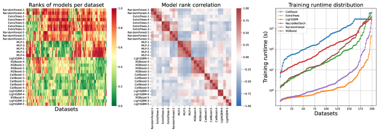
Figure 1: Cluster map of model rank for all datasets (left), correlation of model ranks (middle) and average runtime distribution over every dataset (right). For readability, only the first 5 configurations of each model family are displayed in the left and middle figures.

4 Comparing HPO and AutoML systems

We now show how TabRepo can be used to analyze the performance of base model families and the effect of tuning hyperparameters with ensembling against recent AutoML systems. All experiments are done at marginal costs given that they just require querying precomputed evaluations and predictions.

4.1 Model error and runtime distributions

In Fig. 1, we start by analyzing the performance of different base models. In particular, the rank of model losses over datasets shows that while some model families dominate in performance on aggregate such as gradient boosted methods CatBoost and LightGBM, in some tasks MLP are better suited. Looking at model correlations, we see interesting patterns as some model families are negatively correlated between each other such as MLP and XGBoost which hints at the potential benefit of ensembling.

Next, we plot the distribution of runtime configurations over all 600 tasks. We see that an order of magnitude separates respectively the training runtime of CatBoost from MLP, XGBoost and LightGBM, with the remaining methods being faster still. Importantly, while CatBoost obtains the strongest average rank among model families, it is also the most expensive which is an important aspect to take into account when considering possible training runtime constraints as we will see later in our experiments.

4.2 Effect of tuning and ensembling on model error

We now compare methods across all tasks by using both ranks and normalized errors. Ranks are computed over the $\mathcal{M}$ different models and all AutoML frameworks. Normalized errors are computed by reporting the relative distance to a topline loss compared to a baseline with

$$\frac{l_{\text{method}}-l_{\text{topline}}}{l_{\text{baseline}}-l_{\text{topline}}}$$

while clipping the denominator to 1e-5 and the final score value to $[0,1]$. We use respectively the top and median score among all scores to set the topline and baseline. The median allows to avoid having scores collapse when one model loss becomes very high which can happen frequently for regression cases in presence of overfitting or numerical instabilities.

Comparison.

In Fig. 2 and Tab. 1, we show respectively the whole distribution and the aggregate of our two metrics across all tasks.

For each model family, we evaluate the default hyperparameter, the best hyperparameter obtained after a random search of 4 hours and an ensemble built on top of the best 20 configurations obtained by this search. As previously seen in Fig. 1, CatBoost dominates other models and LightGBM is the runner-up.

In Fig. 2, we see that tuning model hyperparameters improves all models while ensembling allows LightGBM to match CatBoost. No model is able to beat state-of-the-art AutoML systems even with tuning and ensembling. This is unsurprising as all state-of-the-art tabular methods considered multiple model families in order to reach good performance and echoes the finding of Erickson et al. (2020).

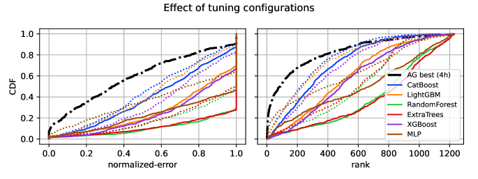
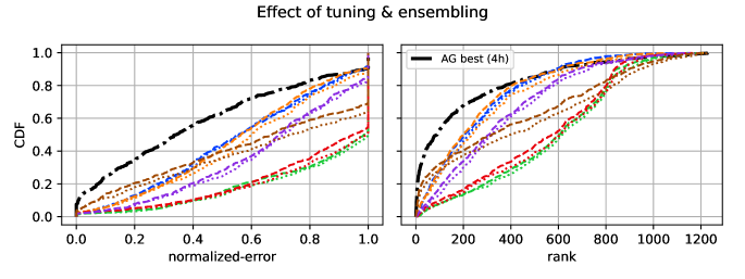
Figure 2: Cumulative distribution function of normalized-errors (left) and ranks (right) for all model families. The line-style denotes respectively the performance of the default configuration (top, solid), of the best configuration after 4h of tuning (top and bottom, dotted) and of an ensemble built on top of the best tuned configurations for the same budget (bottom, dashed).

Table 1: Normalized-error, rank, training and inference time averaged over all tasks given 4h training budget. Inference time is calculated as the prediction time on the test data divided by the number of rows in the test data.

	normalized-error	rank	time fit (s)	time infer (s)
method
Portfolio (ensemble)	0.394	172.0	6715.5	0.050
AutoGluon best	0.406	203.6	5565.3	0.062
Portfolio	0.462	230.7	6715.3	0.012
Autosklearn2	0.476	238.6	14415.9	0.013
AutoGluon high	0.482	276.6	5435.3	0.002
Lightautoml	0.490	240.8	9188.0	0.298
Flaml	0.531	310.1	14269.8	0.002
H2oautoml	0.544	329.9	13920.0	0.002
AutoGluon medium	0.549	304.7	367.7	0.001
CatBoost (tuned + ensemble)	0.557	260.6	9120.8	0.011
LightGBM (tuned + ensemble)	0.559	257.5	3507.5	0.009
CatBoost (tuned)	0.562	272.9	9124.4	0.002
LightGBM (tuned)	0.591	294.6	3527.2	0.001
MLP (tuned + ensemble)	0.610	394.5	5781.3	0.101
CatBoost (default)	0.614	332.4	443.7	0.002
MLP (tuned)	0.646	441.1	5775.5	0.014
XGBoost (tuned + ensemble)	0.657	346.7	4973.8	0.013
XGBoost (tuned)	0.670	368.4	4964.7	0.002
LightGBM (default)	0.747	478.7	54.2	0.001
XGBoost (default)	0.768	509.4	73.2	0.002
MLP (default)	0.782	611.3	39.7	0.015
ExtraTrees (tuned + ensemble)	0.800	526.1	597.4	0.001
ExtraTrees (tuned)	0.818	553.5	597.6	0.000
RandomForest (tuned + ensemble)	0.819	558.7	1507.9	0.001
RandomForest (tuned)	0.830	575.8	1507.3	0.000
ExtraTrees (default)	0.889	762.3	3.8	0.000
RandomForest (default)	0.896	749.4	17.5	0.000

Table 2: Win rate comparison for 4 hour time limit with the same methodology as Erickson et al. (2020). Win rate is computed against a portfolio ensemble (ties count as 0.5). The re-scaled loss is calculated by setting the best solution to 0 and the worst solution to 1 on each dataset, and then normalizing and taking the mean across all datasets. Rank, fit time, and infer time are averaged over all tasks.

method	winrate	$>$	$<$	=	time fit (s)	time infer (s)	loss (rescaled)	rank
Portfolio (ensemble) (4h)	0.500			200	6722.4	0.050	0.253	3.192
AutoGluon best (4h)	0.465	91	105	4	5565.3	0.062	0.287	3.433
Autosklearn2 (4h)	0.378	74	123	3	14415.9	0.013	0.395	4.330
Lightautoml (4h)	0.270	52	144	4	9188.0	0.298	0.429	4.638
CatBoost (tuned + ensemble) (4h)	0.235	46	152	2	9128.3	0.009	0.508	4.995
Autosklearn (4h)	0.302	59	138	3	14413.6	0.009	0.509	5.053
Flaml (4h)	0.310	60	136	4	14269.8	0.002	0.530	5.055
H2oautoml (4h)	0.233	45	152	3	13920.0	0.002	0.555	5.305

5 Portfolio learning with TabRepo

In the previous section, we saw how TabRepo can be leveraged to analyze the performance of frameworks when performing tuning and ensembling. In particular, we saw that ensembling a model family after tuning does not outperform current AutoML systems. We now show how TabRepo can be combined with transfer learning techniques to perform the tuning search offline and outperform current AutoML methods.

Portfolio learning.

To leverage offline data and speed-up model selection, Xu et al. (2010) proposed an approach to learn a portfolio of complementary configurations that performs well on average when evaluating all the configurations of the portfolio and selecting the best one.

Similarly to Caruana ensemble selection described in Eq. 4, the method iteratively selects $\mathcal{N}<\mathcal{M}$ configurations as follows

$$j_{1}=\operatorname*{arg\,min}_{j_{1}\in[\mathcal{M}]}{\mathbb{E}_{i\sim[\mathcal{T}]}[{\ell_{ij_{1}}}^{(\text{train})}]},\quad\quad j_{n}=\operatorname*{arg\,min}_{j_{n}\in[\mathcal{M}]}{\mathbb{E}_{i\sim[\mathcal{T}]}[~{}\min_{k\in[n]}{\ell_{ij_{k}}}^{(\text{train})}}].$$

At each iteration, the method greedily picks the configuration that has the lowest average error when combined with previously selected portfolio configuration.

Anytime portfolio.

Fitting portfolio configurations can be done in an any-time fashion given a fitting time budget. To do so, we evaluate portfolio configurations sequentially until the budget is exhausted and use only models trained up to this point to select an ensemble. In cases where the first configuration selected by the portfolio takes longer to run than the constraint, we instead report the result of a fast baseline as in Gijsbers et al. (2019).

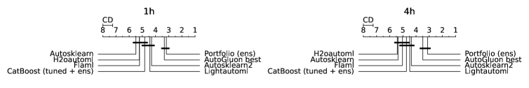
Figure 3: Top: scatter plot of average normalized error (left) and rank (right) against fitting training time budget. Bottom: Critical difference (CD) diagram showing average rank between method selected and which methods are tied statistically by a horizontal bar.

Evaluations.

We evaluate the anytime portfolio approach in a standard leave-one-out setting. When evaluating on the $i$-th dataset, we compute portfolio configurations on $\mathcal{D}-1$ training datasets by excluding the $i$-th test dataset to avoid potential leakage.

Results are reported in Tab. 1 when considering a 4h fitting budget constraint. We report both the performance of the best model according to validation error (”Portfolio”) and when ensembling the selected portfolio configurations (”Portfolio (ensemble)”). The portfolio combined with ensembling outperforms AutoGluon for accuracy and latency given the same 4h fitting budget even without stacking. When only picking the best model without ensembling, the portfolio still retains good performance and outperforms all frameworks other than AutoGluon while having a very low latency. We also report win rate following the methodology of Erickson et al. (2020) in Tab. 2 which confirms the same result, namely the portfolio obtained from TabRepo outperforms other AutoML methods.

In Fig. 3, we report the performance for different fitting budgets. Ensembles of portfolio configurations can beat all AutoML frameworks for all metrics for 1h, 4h and 24h budget without requiring stacking which allows to obtain a lower latency compared to AutoGluon. Critical difference (CD) diagrams from Demšar (2006) show that while portfolio has better aggregate performance than other methods, AutoGluon and Portfolio are tied statistically. Those two methods are the only methods that are statistically better than all baselines. Interestingly among AutoML systems besides AutoGluon, only AutoSklearn 2 and LightAutoML are better than a baseline consisting of tuning and ensembling CatBoost models although the methods are tied statistically to this baseline.

As in the previous section, all evaluations are obtained from pre-computed results in TabRepo. This demonstrates another potential use of TabRepo, namely to be able to design a system combining transfer learning and ensembling that can reach state-of-the-art performance and compare against a wide variety of methods at marginal compute cost.

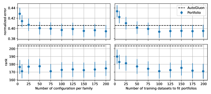
Figure 4: Effect of number of configuration per family (left) and number of training dataset (right) on normalized-error (top) and rank (bottom). All methods are fitted under a 4h fitting budget.

How much data is needed?

We have seen that TabRepo allows to learn portfolio configurations that can outperform state-of-the-art AutoML systems. Next, we analyze the question of how much data is needed for transfer learning to achieve strong results in two dimensions, namely: how many offline configurations and datasets are required to reach good performance? While important, these dimensions are rarely analyzed in previous transfer learning studies due to their significant cost, however they can be obtained in a cheap fashion with TabRepo.

In Fig. 4, we vary both of those dimensions independently. When evaluating on a test dataset, we pick a random subset of configurations $\mathcal{M}{}^{\prime}$ per model family in the first case and a random subset of $\mathcal{D}^{\prime}<\mathcal{D}$ datasets in the second case and report mean and standard error over 10 different seeds. Portfolio with ensembling starts outperforming AutoGluon at around 50 configurations or datasets. Having more datasets or more configurations in offline data both improve the final performance up to a certain point with a saturating effect around 100 offline configurations or offline datasets.

6 Limitations

Cost.

Evaluating offline configurations is expensive. In total, 26592 hours on a m6i.2xlarge instance on AWS were needed to complete all model evaluations of TabRepo which translates to 212736 CPU hours. However, performing the analysis done in this paper without leveraging precomputed evaluations and predictions would have costed 86415 hours on a m6i.2xlarge which translates to 691320 CPU hours which is $\sim 3.2{}$ times more expensive. We hope that the repository can be used to test more research ideas which would further amortize its cost.

Dataset features.

While previous works were able to demonstrate improvements when taking dataset features (Feurer et al., 2015b; Jomaa et al., 2021), we were not able to obtain similar improvement over simple portfolio methods. We postulate this may be due to a need of human feature engineering or it may also be that the large number of datasets used to learn the portfolios makes conditioning on dataset features less critical as seen in (Feurer et al., 2020).

Transformers.

We did not include transformer models e.g. (Gorishniy et al., 2021) as their training cost can be significantly higher and their performance against other tabular methods such as Gradient Boosted Trees is still being investigated (Grinsztajn et al., 2022).

7 Conclusion

In this paper, we introduced TabRepo, a benchmark of tabular models on a large number of datasets. Critically, the repository contains not only model evaluations but also predictions which allows to efficiently evaluate ensemble strategies. We showed that the benchmark can be used to analyze at no cost the performance of different tuning strategies combined with ensembling. We also showed how the dataset can be used to learn portfolio configurations that outperforms state-of-the-art tabular methods for accuracy, training time and latency.

The code for accessing evaluations from TabRepo and evaluating any ensemble will be made available with the camera ready together with the scripts used to generate all the paper results. We hope this paper will facilitate future research on new methods combining ideas from CASH, multi-fidelity and transfer-learning to further improve the state-of-the-art in tabular predictions.

Acknowledgments

We thank Garrett Idler for his contribution to make the computation of the receiver operating characteristic curve much faster in C++ and also Wenming Ye, Cedric Archambeau and Jacek Golebiovski for their support. Finally, we thank OpenML and AutoMLBenchmark which were very important for this work.

Appendix A Additional experiment details

Number of Caruana Steps.

In all our experiments, we set the number of Caruana steps to $\mathcal{C}{}=40$ when building ensembles of base models or portfolio configurations. We observe that values beyond 40 provide negligible benefit while linearly increasing the runtime of simulations in TabRepo.

Fallback method.

We use the default configuration of Extra-trees as a backup when the first configuration of a portfolio does not finish under the constraint which takes just a few seconds to evaluate.

Number of portfolio configurations.

When reporting results on a portfolio, we apply the anytime procedure described in Sec 5 and run at most $\mathcal{N}=200$ portfolio configurations. Setting this bound serves mostly as an upper-bound as all configurations are almost never evaluated given that all configurations have to be trained under the fitting budget. We investigate the effect of increasing the number of portfolio configurations in Fig. 5.

Hardware details.

All model configuration and AutoML framework results were obtained on AWS EC2 machines via AutoMLBenchmark’s AWS mode functionality. For all model and AutoML evaluations, we used m6i.2xlarge EC2 instances with 100 GB of gp3 storage. These instances have 8 virtual CPUs (4 physical CPUs) and 32 GB of memory. The Python version used for all experiments was 3.9.18. We chose m6i.2xlarge instances to align with the AutoMLBenchmark’s choice of m5.2xlarge instances. m5 instances have the same number of CPUs and memory, but the m6i instances were more cost-efficient due to faster CPUs.

All simulation paper experiments in Sec. 4 and 5 were done on a m6i.32xlarge to avoid memory issues and take less than one hour.

Critical difference diagrams.

We use Autorank (Herbold, 2020) to compute critical difference diagrams.

Appendix B API

In Listing 1, we show an example of calling TabRepo to retrieve the ensemble performance of a list of models. Because we store all model predictions, we are able to reconstruct the metrics of any ensemble among the $\mathcal{M}{}=1206{}$ models considered.

⬇

1from tabrepo import EvaluationRepository

2

3# load TabRepo with 200 datasets, 3 folds and 1416 configurations

4repository = EvaluationRepository.from_context(version="D244_F3_C1416_200")

5

6# returns in ~2s the tensor of metrics for each dataset/fold obtained after ensembling the given configurations

7metrics = repository.evaluate_ensemble(

8 datasets=["balance-scale", "page-blocks"], # dataset to report results on

9 folds=[0, 1, 2], # which folds to consider for each dataset

10 configs=["CatBoost_r42_BAG_L1", "NeuralNetTorch_r40_BAG_L1"], # configs that are ensembled

11 ensemble_size=40, # maximum number of Caruana steps

12)

13

14# returns the predictions on the val data for a given task and config

15val_predictions = repository.predict_val(

16 dataset="page-blocks", fold=2, config="ExtraTrees_r7_BAG_L1"

17)

18

19# returns the predictions on the test data for a given task and config

20test_predictions = repository.predict_test(

21 dataset="page-blocks", fold=2, config="ExtraTrees_r7_BAG_L1"

22)

Listing 1: Example of calling TabRepo to obtain performance scores on an ensemble configuration or model predictions on validation/test splits.

Appendix C Dataset details

For selecting the datasets, we combined two prior tabular dataset suites. The first is from the AutoMLBenchmark (Gijsbers et al., 2022), containing 104 datasets. The second is from the Auto-Sklearn 2 paper (Feurer et al., 2020), containing 208 datasets.

All datasets are publicly available via OpenML. After de-duplicating, the union contains 289 datasets. The AutoMLBenchmark datasets have been previously filtered from a larger set via a specific inclusion criteria detailed in section 5.1.1 of Gijsbers et al. (2022). Notably, they filter out datasets that are trivial, such that simple methods such as a random forest cannot perfectly solve them. We perform a similar operation by fitting a default Random Forest configuration on all 289 datasets and filtering any dataset that is trivial (AUC $>$ 0.999, log loss $<$ 0.001, or r2 $>$ 0.999). After filtering trivial datasets, we are left with 244 datasets.

We then run all AutoML baselines and model configurations on the 244 datasets (3 folds, for a total of 732 tasks). We performed re-runs on failed tasks when necessary to attempt to get results on all models and AutoML systems for every dataset, but sometimes this was not possible due to problems such as out-of-memory errors or AutoML system implementation errors outside our control. For datasets with model or AutoML system failures, we exclude them. We exclude datasets rather than impute missing values to ensure the results being computed are fully verifiable and replicable in practice. After excluding datasets with model or AutoML system failures, we have 211 datasets remaining.

Finally, we filter out the 11 largest datasets for practical usability purposes of TabRepo. This is because loading the prediction probabilities of 1206 model configurations on large (multi-class) datasets leads to significant challenges. As an example, the total size of the predictions for 211 datasets is 455 GB. By reducing to 200 datasets, the size decreases dramatically to 107 GB (The full 244 datasets is 4.5 TB).

In total, we use 105 binary classification datasets, 67 multi-class classification datasets and 28 regression datasets. We provide a table of dataset summary statistics in Tab. 3 and an exhaustive list of the 200 datasets used in TabRepo separated by problem type in Tab. 4, Tab. 5 and Tab. 6 where we list for each dataset the TaskID OpenML identifier, the dataset name, the number of rows $n$, the number of features $f$ and the number of classes $C$ which is always 2 for binary classification.

C.1 Train-test splits

For all datasets we use the OpenML 10-fold Cross-validation estimation procedure and select the first 3 folds for our experiments. For each task (a particular dataset fold), we use 90% of the data as training and 10% as test. We use identical splits to Gijsbers et al. (2022).

Table 3: Statistics of the 200 datasets in TabRepo

	n	f
mean	17722	570
std	55270	2161
min	100	3
5%	500	3
10%	575	5
25%	1107	10
50%	3800	20
75%	10027	60
90%	41173	506
95%	73134	1787
max	583250	10936

Table 4: Binary classification datasets used in TabRepo.

Task ID	name	n	f	C	Task ID	name	n	f	C
3593	2dplanes	40768	10	2	3783	fri_c2_500_50	500	50	2
168868	APSFailure	76000	170	2	3606	fri_c3_1000_10	1000	10	2
359979	Amazon_employee_acce	32769	9	2	3581	fri_c3_1000_25	1000	25	2
146818	Australian	690	14	2	3799	fri_c3_500_10	500	10	2
359967	Bioresponse	3751	1776	2	3800	fri_c3_500_50	500	50	2
359992	Click_prediction_sma	39948	11	2	3608	fri_c4_500_100	500	100	2
361331	GAMETES_Epistasis_2-	1600	1000	2	3764	fried	40768	10	2
361332	GAMETES_Epistasis_2-	1600	20	2	189922	gina	3153	970	2
361333	GAMETES_Epistasis_2-	1600	20	2	9970	hill-valley	1212	100	2
361334	GAMETES_Epistasis_3-	1600	20	2	3892	hiva_agnostic	4229	1617	2
361335	GAMETES_Heterogeneit	1600	20	2	3688	houses	20640	8	2
361336	GAMETES_Heterogeneit	1600	20	2	9971	ilpd	583	10	2
359966	Internet-Advertiseme	3279	1558	2	168911	jasmine	2984	144	2
359990	MiniBooNE	130064	50	2	3904	jm1	10885	21	2
3995	OVA_Colon	1545	10935	2	359962	kc1	2109	21	2
3976	OVA_Endometrium	1545	10935	2	3913	kc2	522	21	2
3968	OVA_Kidney	1545	10935	2	3704	kdd_el_nino-small	782	8	2
3964	OVA_Lung	1545	10935	2	3844	kdd_internet_usage	10108	68	2
4000	OVA_Ovary	1545	10935	2	359991	kick	72983	32	2
3980	OVA_Prostate	1545	10936	2	3672	kin8nm	8192	8	2
359971	PhishingWebsites	11055	30	2	190392	madeline	3140	259	2
361342	Run_or_walk_informat	88588	6	2	9976	madelon	2600	500	2
359975	Satellite	5100	36	2	3483	mammography	11183	6	2
125968	SpeedDating	8378	120	2	3907	mc1	9466	38	2
361339	Titanic	2201	3	2	3623	meta	528	21	2
190411	ada	4147	48	2	3899	mozilla4	15545	5	2
359983	adult	48842	14	2	3749	no2	500	7	2
3600	ailerons	13750	40	2	359980	nomao	34465	118	2
190412	arcene	100	10000	2	167120	numerai28.6	96320	21	2
3812	arsenic-female-bladd	559	4	2	190137	ozone-level-8hr	2534	72	2
9909	autoUniv-au1-1000	1000	20	2	361341	parity5_plus_5	1124	10	2
359982	bank-marketing	45211	16	2	3667	pbcseq	1945	18	2
3698	bank32nh	8192	32	2	3918	pc1	1109	21	2
3591	bank8FM	8192	8	2	3919	pc2	5589	36	2
359955	blood-transfusion-se	748	4	2	3903	pc3	1563	37	2
3690	boston_corrected	506	20	2	359958	pc4	1458	37	2
359968	churn	5000	20	2	190410	philippine	5832	308	2
146819	climate-model-simula	540	20	2	168350	phoneme	5404	5	2
3793	colleges_usnews	1302	33	2	3616	pm10	500	7	2
3627	cpu_act	8192	21	2	3735	pollen	3848	5	2
3601	cpu_small	8192	12	2	3618	puma32H	8192	32	2
168757	credit-g	1000	20	2	3681	puma8NH	8192	8	2
14954	cylinder-bands	540	39	2	359956	qsar-biodeg	1055	41	2
3668	delta_ailerons	7129	5	2	9959	ringnorm	7400	20	2
3684	delta_elevators	9517	6	2	3583	rmftsa_ladata	508	10	2
37	diabetes	768	8	2	43	spambase	4601	57	2
125920	dresses-sales	500	12	2	359972	sylvine	5124	20	2
9983	eeg-eye-state	14980	14	2	361340	tokyo1	959	44	2
219	electricity	45312	8	2	9943	twonorm	7400	20	2
3664	fri_c0_1000_5	1000	5	2	3786	visualizing_soil	8641	4	2
3747	fri_c0_500_5	500	5	2	146820	wilt	4839	5	2
3702	fri_c1_1000_50	1000	50	2	3712	wind	6574	14	2
3766	fri_c2_1000_25	1000	25	2

Table 5: Multi-class classification datasets used in TabRepo.

Task ID	name	n	f	C	Task ID	name	n	f	C
211986	Diabetes130US	101766	49	3	6	letter	20000	16	26
359970	GesturePhaseSegmenta	9873	32	5	359961	mfeat-factors	2000	216	10
360859	Indian_pines	9144	220	8	359953	micro-mass	571	1300	20
125921	LED-display-domain-7	500	7	10	189773	microaggregation2	20000	20	5
146800	MiceProtein	1080	81	8	359993	okcupid-stem	50789	19	3
361330	Traffic_violations	70340	20	3	28	optdigits	5620	64	10
168300	UMIST_Faces_Cropped	575	10304	20	30	page-blocks	5473	10	5
3549	analcatdata_authorsh	841	70	4	32	pendigits	10992	16	10
3560	analcatdata_dmft	797	4	6	359986	robert	10000	7200	10
14963	artificial-character	10218	7	10	2074	satimage	6430	36	6
9904	autoUniv-au6-750	750	40	8	359963	segment	2310	19	7
9906	autoUniv-au7-1100	1100	12	5	9964	semeion	1593	256	10
9905	autoUniv-au7-700	700	12	3	359987	shuttle	58000	9	7
11	balance-scale	625	4	3	41	soybean	683	35	19
2077	baseball	1340	16	3	45	splice	3190	60	3
359960	car	1728	6	4	168784	steel-plates-fault	1941	27	7
9979	cardiotocography	2126	35	10	3512	synthetic_control	600	60	6
359959	cmc	1473	9	3	125922	texture	5500	40	11
359957	cnae-9	1080	856	9	190146	vehicle	846	18	4
146802	collins	1000	23	30	9924	volcanoes-a2	1623	3	5
359977	connect-4	67557	42	3	9925	volcanoes-a3	1521	3	5
168909	dilbert	10000	2000	5	9926	volcanoes-a4	1515	3	5
359964	dna	3186	180	3	9927	volcanoes-b1	10176	3	5
359954	eucalyptus	736	19	5	9928	volcanoes-b2	10668	3	5
3897	eye_movements	10936	27	3	9931	volcanoes-b5	9989	3	5
168910	fabert	8237	800	7	9932	volcanoes-b6	10130	3	5
359969	first-order-theorem-	6118	51	6	9920	volcanoes-d1	8753	3	5
14970	har	10299	561	6	9923	volcanoes-d4	8654	3	5
3481	isolet	7797	617	26	9915	volcanoes-e1	1183	3	5
211979	jannis	83733	54	4	9960	wall-robot-navigatio	5456	24	4
359981	jungle_chess_2pcs_ra	44819	6	3	58	waveform-5000	5000	40	3
9972	kr-vs-k	28056	6	18	361345	wine-quality-red	1599	11	6
2076	kropt	28056	6	18	359974	wine-quality-white	4898	11	7
361344	led24	3200	24	10

Table 6: Regression datasets used in TabRepo.

Task ID	name	n	f	Task ID	name	n	f
233212	Allstate_Claims_Seve	188318	130	359936	elevators	16599	18
359938	Brazilian_houses	10692	12	359952	house_16H	22784	16
233213	Buzzinsocialmedia_Tw	583250	77	359951	house_prices_nominal	1460	79
360945	MIP-2016-regression	1090	144	359949	house_sales	21613	21
233215	Mercedes_Benz_Greene	4209	376	359946	pol	15000	48
167210	Moneyball	1232	14	359930	quake	2178	3
359941	OnlineNewsPopularity	39644	59	359931	sensory	576	11
359948	SAT11-HAND-runtime-r	4440	116	359932	socmob	1156	5
317614	Yolanda	400000	100	359933	space_ga	3107	6
359944	abalone	4177	8	359934	tecator	240	124
359937	black_friday	166821	9	359939	topo_2_1	8885	266
359950	boston	506	13	359945	us_crime	1994	126
359942	colleges	7063	44	359935	wine_quality	6497	11
233211	diamonds	53940	9	359940	yprop_4_1	8885	251

Appendix D Model details

For each model type, we used the latest available package versions when possible. The precise versions used for each model are documented in Tab. 7.

Table 7: Model versions.

model	benchmarked	latest	package
LightGBM	3.3.5	4.0.0	lightgbm
XGBoost	1.7.6	2.0.0	xgboost
CatBoost	1.2.1	1.2.2	catboost
RandomForest	1.1.1	1.3.1	scikit-learn
ExtraTrees	1.1.1	1.3.1	scikit-learn
MLP	2.0.1	2.0.1	torch

For each model family, we choose 201 configurations, 1 being the default hyperparameters, as well as 200 randomly selected hyperparameter configs.

The search spaces used are based on the search spaces defined in AutoGluon. We expanded the search range of various hyperparameters for increased model variety. Note that selecting the appropriate search space is a complex problem, and is not the focus of this work. TabRepo is built to work with arbitrary model configurations, and we welcome the research community to improve upon our initial baselines.

For all models we re-use the AutoGluon implementation for data pre-processing, initial hyperparameters, training, and prediction. We do this because choosing the appropriate pre-processing logic for an individual model is complex and introduces a myriad of design questions and potential pitfalls.

For maximum training epochs / iterations, instead of searching for an optimal value directly, we instead rely on the early stopping logic implemented in AutoGluon which sets the iterations to 10,000 for gradient boosting models and epochs to 500 for MLP.

D.1 Model Config Full Results

Refer to the supplementary file results_ranked_configs.csv for the complete set of results for all model configs on all tasks. This file includes the training runtime, inference time (per row), and metric error for all models on each task.

D.2 Model Config Hyperparameters

Refer to the supplementary files located in the folder configs/ for the hyperparameters used for each model config.

D.3 MLP

⬇

1{

2 ’learning_rate’: Real(1e-4, 3e-2, default=3e-4, log=True),

3 ’weight_decay’: Real(1e-12, 0.1, default=1e-6, log=True),

4 ’dropout_prob’: Real(0.0, 0.4, default=0.1),

5 ’use_batchnorm’: Categorical(False, True),

6 ’num_layers’: Int(1, 5, default=2),

7 ’hidden_size’: Int(8, 256, default=128),

8 ’activation’: Categorical(’relu’, ’elu’),

9}

D.4 CatBoost

⬇

1{

2 ’learning_rate’: Real(lower=5e-3, upper=0.1, default=0.05, log=True),

3 ’depth’: Int(lower=4, upper=8, default=6),

4 ’l2_leaf_reg’: Real(lower=1, upper=5, default=3),

5 ’max_ctr_complexity’: Int(lower=1, upper=5, default=4),

6 ’one_hot_max_size’: Categorical(2, 3, 5, 10),

7 ’grow_policy’: Categorical("SymmetricTree", "Depthwise")

8}

D.5 LightGBM

⬇

1{

2 ’learning_rate’: Real(lower=5e-3, upper=0.1, default=0.05, log=True),

3 ’feature_fraction’: Real(lower=0.4, upper=1.0, default=1.0),

4 ’min_data_in_leaf’: Int(lower=2, upper=60, default=20),

5 ’num_leaves’: Int(lower=16, upper=255, default=31),

6 ’extra_trees’: Categorical(False, True),

7}

D.6 XGBoost

⬇

1{

2 ’learning_rate’: Real(lower=5e-3, upper=0.1, default=0.1, log=True),

3 ’max_depth’: Int(lower=4, upper=10, default=6),

4 ’min_child_weight’: Real(0.5, 1.5, default=1.0),

5 ’colsample_bytree’: Real(0.5, 1.0, default=1.0),

6 ’enable_categorical’: Categorical(True, False),

7}

D.7 Extra-trees

For all Extra Trees models we use 300 trees.

⬇

1{

2 ’max_leaf_nodes’: Int(5000, 50000),

3 ’min_samples_leaf’: Categorical(1, 2, 3, 4, 5, 10, 20, 40, 80),

4 ’max_features’: Categorical(’sqrt’, ’log2’, 0.5, 0.75, 1.0)

5}

D.8 Random-forest

For all Random Forest models we use 300 trees.

⬇

1{

2 ’max_leaf_nodes’: Int(5000, 50000),

3 ’min_samples_leaf’: Categorical(1, 2, 3, 4, 5, 10, 20, 40, 80),

4 ’max_features’: Categorical(’sqrt’, ’log2’, 0.5, 0.75, 1.0)

5}

Appendix E AutoML Framework Details

For each AutoML framework we attempted to use the latest available versions where possible. The precise versions used for each framework are documented in Tab. 8. For FLAML, version 2.0 released after we had ran the experiments.

E.1 AutoML Framework Full Results

Refer to the supplementary file results_ranked_automl.csv for the complete set of results for all AutoML systems on all tasks. This file includes the training runtime, inference time (per row), and metric error for each task.

E.2 Auto-Sklearn 2

Meta-Learning.

Auto-Sklearn 2 uses meta-learning to improve the quality of its results. Since the datasets used to train its meta-learning algorithm are present in TabRepo, the performance of Auto-Sklearn 2 may be overly optimistic as it may be choosing to train model hyperparameters known to achieve strong test scores on a given dataset. This issue is detailed in section 5.3.3 of Gijsbers et al. (2022). Following Gijsbers et al. (2022), we ultimately decide to keep Auto-Sklearn 2’s results as a useful comparison point.

Regression.

Auto-Sklearn 2 is incompatible with regression tasks. For regression tasks, we use the result from Auto-Sklearn 1.

Table 8: AutoML framework versions.

framework	benchmarked	latest	package
AutoGluon	0.8.2	0.8.2	autogluon
auto-sklearn	0.15.0	0.15.0	auto-sklearn
auto-sklearn 2	0.15.0	0.15.0	auto-sklearn
FLAML	1.2.4	2.1.0	flaml
H2O AutoML	3.40.0.4	3.42.0.3	h2o
LightAutoML	0.3.7.3	0.3.7.3	lightautoml

Appendix F Additional results Portfolios

F.1 Portfolio win-rate comparison

We calculate win-rates, re-scaled loss, and average ranks between the Portfolio and the AutoML systems in Tab. 10 and Tab. 2 for 1 and 4 hour time limits respectively with the same evaluation protocol as Erickson et al. (2020). In both cases, Portfolio achieves the best win-rate, re-scaled loss, and average rank across all methods at the given time constraint.

F.2 Effect of runtime and number of portfolio configurations

In Fig. 5, we show the effect of increasing the time budget bound and the number of portfolio configuration bound $\mathcal{N}{}$. Increasing the fitting time limit yields constant improvement however increasing the number of portfolio configurations provides quickly diminishing returns given that a large number of configurations can rarely be evaluated given a reasonable time limit except for very small datasets.

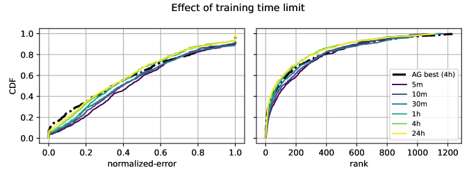
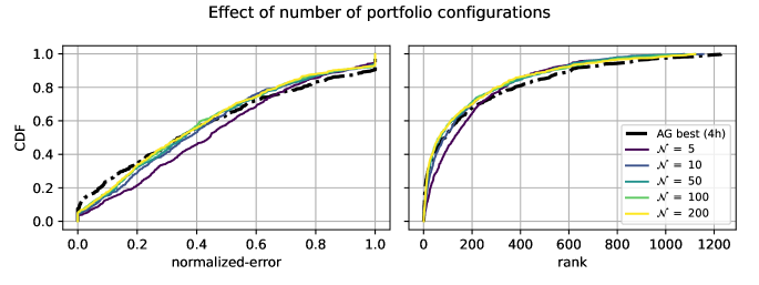
Figure 5: Effect on performance of fitting time (top) and number of portfolio configurations (bottom). In the second case, portfolios are fitted with a 4h fitting budget.

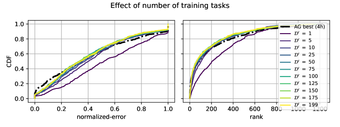
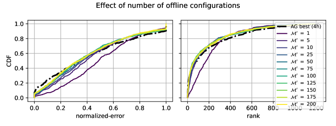
Figure 6: From top to bottom, effect of the number of training datasets and offline configurations per model family on distribution performance. All methods are fitted under a 4h fitting budget.

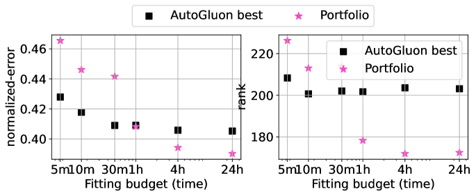
Figure 7: Scatter plot of average normalized error (left) and rank (right) against fitting smaller training time budget for portfolio and AutoGluon.

F.3 Performance on lower fitting budgets

In section 5, we reported results for 1h, 4h fitting budgets which are standard settings (Erickson et al., 2020; Gijsbers et al., 2022). Given space constraint, we only showed the full table for 4h results in the main, the results for 1h results is shown in Tab. 9. Here the anytime portfolio strategy matches AutoGluon on normalized-error and outperforms it on rank while having around 30% lower latency.

Table 9: Normalized-error, rank, training and inference time averaged over all tasks given 1h training budget.

	normalized-error	rank	time fit (s)	time infer (s)
method
Portfolio (ensemble)	0.408	178.3	2435.0	0.023
AutoGluon best	0.409	201.6	2283.6	0.033
AutoGluon high	0.477	273.1	2201.2	0.002
Autosklearn2	0.494	254.1	3611.2	0.010
Lightautoml	0.503	246.4	3007.9	0.099
H2oautoml	0.547	316.5	3572.8	0.002
Flaml	0.550	330.1	3622.9	0.001
AutoGluon medium	0.551	306.5	270.5	0.001
LightGBM (tuned + ensemble)	0.563	260.5	1622.5	0.009
CatBoost (tuned + ensemble)	0.576	281.8	2873.5	0.005
CatBoost (tuned)	0.588	296.0	2884.7	0.002
LightGBM (tuned)	0.597	300.7	1627.9	0.002
CatBoost (default)	0.614	332.4	443.7	0.002
MLP (tuned + ensemble)	0.622	405.1	2560.2	0.107
MLP (tuned)	0.653	447.2	2559.8	0.014
XGBoost (tuned + ensemble)	0.662	356.5	1860.1	0.012
XGBoost (tuned)	0.675	379.1	1856.6	0.002
LightGBM (default)	0.747	478.7	54.2	0.001
XGBoost (default)	0.768	509.4	73.2	0.002
MLP (default)	0.782	611.3	39.7	0.015
ExtraTrees (tuned + ensemble)	0.799	525.4	386.9	0.001
ExtraTrees (tuned)	0.818	553.7	386.8	0.000
RandomForest (tuned + ensemble)	0.818	559.0	676.4	0.001
RandomForest (tuned)	0.830	575.6	671.8	0.000
ExtraTrees (default)	0.889	762.3	3.8	0.000
RandomForest (default)	0.896	749.4	17.5	0.000

Table 10: Win rate comparison for 1 hour time limit with the same approach used as for Tab. 2.

method	winrate	$>$	$<$	=	time fit (s)	time infer (s)	loss (rescaled)	rank
Portfolio (ensemble) (1h)	0.500			200	2434.9	0.023	0.250	3.257
AutoGluon best (1h)	0.487	95	100	5	2283.6	0.033	0.273	3.308
Autosklearn2 (1h)	0.380	74	122	4	3611.2	0.010	0.392	4.280
Lightautoml (1h)	0.307	59	136	5	3007.9	0.099	0.411	4.423
CatBoost (tuned + ensemble) (1h)	0.233	45	152	3	2876.2	0.004	0.518	5.122
H2oautoml (1h)	0.263	51	146	3	3572.8	0.002	0.513	5.128
Autosklearn (1h)	0.310	60	136	4	3612.0	0.007	0.545	5.185
Flaml (1h)	0.278	53	142	5	3622.9	0.001	0.559	5.298

In Fig. 7, we also report the performance for 5m, 10m, 30m budgets in addition to 1h, 4h and 24h for both portfolio ensembles and AutoGluon. For budgets lower than 1h, we select portfolio configurations only among configurations whose runtime are under the constraint at least 95% of the time on available training datasets. For budgets lower than 1h, the performance of portfolio drops significantly. However, this result is overly pessimistic. Indeed, whenever the first configuration selected by the portfolio does not finish before the constraint, we return the result of a cheap baseline as we do not store all model checkpoints whereas AutoGluon instead uses the best checkpoint found until that point. To allow simulation under those cheaper settings, one would have to store more checkpoints per model (for instance at a 10 minute frequency or at 5m, 10m, 30m and 1h time points as done in Borchert et al. (2022)) but we decided against this option as the storage cost of TabRepo is already significant (roughly 107 GB).

References

- Arango et al. (2023) Sebastian Pineda Arango, Fabio Ferreira, Arlind Kadra, and Frank Hutter Josif Grabocka. Quick-tune: Quickly learning which pretrained model to finetune and how. arXiv preprint arXiv:2306.03828, 2023.
- Borchert et al. (2022) Oliver Borchert, David Salinas, Valentin Flunkert, Tim Januschowski, and Stephan Günnemann. Multi-objective model selection for time series forecasting, 2022.
- Breiman (1996) Leo Breiman. Bagging predictors. Machine learning, 24:123–140, 1996.
- Breiman (2001) Leo Breiman. Random forests. Machine learning, 45:5–32, 2001.
- Caruana et al. (2004) Rich Caruana, Alexandru Niculescu-Mizil, Geoff Crew, and Alex Ksikes. Ensemble selection from libraries of models. In Proceedings of the twenty-first international conference on Machine learning, pp. 18, 2004.
- Chen & Guestrin (2016) Tianqi Chen and Carlos Guestrin. Xgboost: A scalable tree boosting system. In Proceedings of the 22nd acm sigkdd international conference on knowledge discovery and data mining, pp. 785–794, 2016.
- Demšar (2006) Janez Demšar. Statistical comparisons of classifiers over multiple data sets. The Journal of Machine learning research, 7:1–30, 2006.
- Dong & Yang (2020) X. Dong and Y. Yang. NAS-Bench-201: Extending the scope of reproducible neural architecture search. Technical Report arXiv:2001.00326 [cs.CV], 2020.
- Eggensperger et al. (2021) Katharina Eggensperger, Philipp Müller, Neeratyoy Mallik, Matthias Feurer, René Sass, Aaron Klein, Noor H. Awad, Marius Lindauer, and Frank Hutter. Hpobench: A collection of reproducible multi-fidelity benchmark problems for HPO. CoRR, abs/2109.06716, 2021. URL https://arxiv.org/abs/2109.06716.
- Erickson et al. (2020) Nick Erickson, Jonas Mueller, Alexander Shirkov, Hang Zhang, Pedro Larroy, Mu Li, and Alexander Smola. Autogluon-tabular: Robust and accurate automl for structured data. 2020.
- Feurer et al. (2015a) Matthias Feurer, Aaron Klein, Katharina Eggensperger, Jost Springenberg, Manuel Blum, and Frank Hutter. Efficient and robust automated machine learning. Advances in neural information processing systems, 28, 2015a.
- Feurer et al. (2015b) Matthias Feurer, Jost Springenberg, and Frank Hutter. Initializing bayesian hyperparameter optimization via meta-learning. Proceedings of the AAAI Conference on Artificial Intelligence, 29(1), Feb. 2015b. doi: 10.1609/aaai.v29i1.9354. URL https://ojs.aaai.org/index.php/AAAI/article/view/9354.
- Feurer et al. (2020) Matthias Feurer, Katharina Eggensperger, Stefan Falkner, Marius Lindauer, and Frank Hutter. Auto-sklearn 2.0: The next generation. arXiv preprint arXiv:2007.04074, 24, 2020.
- Friedman (2001) Jerome H Friedman. Greedy function approximation: a gradient boosting machine. Annals of statistics, pp. 1189–1232, 2001.
- Geurts et al. (2006) Pierre Geurts, Damien Ernst, and Louis Wehenkel. Extremely randomized trees. Machine learning, 63:3–42, 2006.
- Gijsbers et al. (2019) Pieter Gijsbers, Erin LeDell, Janek Thomas, Sébastien Poirier, Bernd Bischl, and Joaquin Vanschoren. An open source automl benchmark. arXiv preprint arXiv:1907.00909, 2019.
- Gijsbers et al. (2022) Pieter Gijsbers, Marcos LP Bueno, Stefan Coors, Erin LeDell, Sébastien Poirier, Janek Thomas, Bernd Bischl, and Joaquin Vanschoren. Amlb: an automl benchmark. arXiv preprint arXiv:2207.12560, 2022.
- Gorishniy et al. (2021) Yury Gorishniy, Ivan Rubachev, Valentin Khrulkov, and Artem Babenko. Revisiting deep learning models for tabular data. Advances in Neural Information Processing Systems, 34:18932–18943, 2021.
- Grinsztajn et al. (2022) Léo Grinsztajn, Edouard Oyallon, and Gaël Varoquaux. Why do tree-based models still outperform deep learning on tabular data?, 2022.
- He et al. (2021) Xin He, Kaiyong Zhao, and Xiaowen Chu. Automl: A survey of the state-of-the-art. Knowledge-Based Systems, 212:106622, 2021.
- Hearst et al. (1998) Marti A. Hearst, Susan T Dumais, Edgar Osuna, John Platt, and Bernhard Scholkopf. Support vector machines. IEEE Intelligent Systems and their applications, 13(4):18–28, 1998.
- Herbold (2020) Steffen Herbold. Autorank: A python package for automated ranking of classifiers. Journal of Open Source Software, 5(48):2173, 2020. doi: 10.21105/joss.02173. URL https://doi.org/10.21105/joss.02173.
- Hollmann et al. (2022) Noah Hollmann, Samuel Müller, Katharina Eggensperger, and Frank Hutter. Tabpfn: A transformer that solves small tabular classification problems in a second. arXiv preprint arXiv:2207.01848, 2022.
- Jomaa et al. (2021) Hadi S Jomaa, Lars Schmidt-Thieme, and Josif Grabocka. Dataset2vec: Learning dataset meta-features. Data Mining and Knowledge Discovery, 35:964–985, 2021.
- Ke et al. (2017) Guolin Ke, Qi Meng, Thomas Finley, Taifeng Wang, Wei Chen, Weidong Ma, Qiwei Ye, and Tie-Yan Liu. Lightgbm: A highly efficient gradient boosting decision tree. Advances in neural information processing systems, 30, 2017.
- Klein & Hutter (2019) A. Klein and F. Hutter. Tabular benchmarks for joint architecture and hyperparameter optimization. Technical Report arXiv:1905.04970 [cs.LG], 2019.
- LeDell & Poirier (2020) Erin LeDell and Sebastien Poirier. H2o automl: Scalable automatic machine learning. In Proceedings of the AutoML Workshop at ICML, volume 2020. ICML, 2020.
- Olson & Moore (2016) Randal S Olson and Jason H Moore. Tpot: A tree-based pipeline optimization tool for automating machine learning. In Workshop on automatic machine learning, pp. 66–74. PMLR, 2016.
- Prokhorenkova et al. (2018) Liudmila Prokhorenkova, Gleb Gusev, Aleksandr Vorobev, Anna Veronika Dorogush, and Andrey Gulin. Catboost: unbiased boosting with categorical features. Advances in neural information processing systems, 31, 2018.
- Purucker & Beel (2022) Lennart Purucker and Joeran Beel. Assembled-openML: Creating efficient benchmarks for ensembles in autoML with openML. In First International Conference on Automated Machine Learning (Late-Breaking Workshop), 2022.
- Vakhrushev et al. (2021) Anton Vakhrushev, Alexander Ryzhkov, Maxim Savchenko, Dmitry Simakov, Rinchin Damdinov, and Alexander Tuzhilin. Lightautoml: Automl solution for a large financial services ecosystem. arXiv preprint arXiv:2109.01528, 2021.
- Vanschoren et al. (2014) Joaquin Vanschoren, Jan N. van Rijn, Bernd Bischl, and Luis Torgo. Openml: Networked science in machine learning. SIGKDD Explor. Newsl., 15(2):49–60, jun 2014. ISSN 1931-0145. doi: 10.1145/2641190.2641198. URL https://doi.org/10.1145/2641190.2641198.
- Wang et al. (2021) Chi Wang, Qingyun Wu, Markus Weimer, and Erkang Zhu. Flaml: A fast and lightweight automl library. Proceedings of Machine Learning and Systems, 3:434–447, 2021.
- Wistuba et al. (2015) Martin Wistuba, Nicolas Schilling, and Lars Schmidt-Thieme. Learning hyperparameter optimization initializations. In 2015 IEEE International Conference on Data Science and Advanced Analytics (DSAA), pp. 1–10, 2015. doi: 10.1109/DSAA.2015.7344817.
- Wolpert (1992) David H Wolpert. Stacked generalization. Neural networks, 5(2):241–259, 1992.
- Xu et al. (2010) Lin Xu, Holger Hoos, and Kevin Leyton-Brown. Hydra: Automatically configuring algorithms for portfolio-based selection. In Proceedings of the AAAI Conference on Artificial Intelligence, volume 24, pp. 210–216, 2010.
- Yang et al. (2020) Antoine Yang, Pedro M. Esperança, and Fabio M. Carlucci. Nas evaluation is frustratingly hard, 2020.
- Ying et al. (2019) Chris Ying, Aaron Klein, Eric Christiansen, Esteban Real, Kevin Murphy, and Frank Hutter. NAS-bench-101: Towards reproducible neural architecture search. In Kamalika Chaudhuri and Ruslan Salakhutdinov (eds.), Proceedings of the 36th International Conference on Machine Learning, volume 97 of Proceedings of Machine Learning Research, pp. 7105–7114. PMLR, 09–15 Jun 2019. URL https://proceedings.mlr.press/v97/ying19a.html.
- Zimmer et al. (2021) Lucas Zimmer, Marius Lindauer, and Frank Hutter. Auto-pytorch tabular: Multi-fidelity metalearning for efficient and robust autodl, 2021.