Light-scattering reconstruction of transparent shapes using neural networks

Abstract

We propose a cheap non-intrusive high-resolution method of visualising transparent or translucent objects which may translate, rotate and change their shape. We propose a method of reconstructing a strongly deformed time-evolving surface from a time-series of noisy clouds of points using a lightweight neural network. We benchmark the method against three different geometries and varying levels of noise and find that the Gaussian curvature is accurately recovered when the noise level is below $2\%$ of the diameter of the surface and the data from distinct regions of the surface do not overlap.

1 Introduction

The problem of visualisation of an object and reconstruction of its surface is encountered in a variety of fields ranging from X-ray tomography in medicine, insect reconstruction in biology [1], quality control in manufacturing [2], computer graphics [3], to the digitisation of archaeological artefacts [4] or in epigraphy to enhance the readability of inscriptions [5]. A common solution is using two-camera stereoscopic methods [6] to reconstruct a visualised object, which performs well provided that the slopes of the visualised surface are small i.e. when all of the area is in direct vision to both cameras. To overcome this major limitation, several methods involving a series of images from many ($>30$) viewpoints have been proposed [7, 8, 9, 10, 11, 3]. Several of these methods require placing an object on a turntable or pinning it to a rotating needle and recording it with one camera [9, 8, 1] from multiple points of view, which is possible only for solid and opaque standalone objects. A significantly more expensive approach involving up to 160 cameras allows for reconstructing the instantaneous shape of objects that can change their shape [3]. However, even these sophisticated methods cannot ensure that the whole surface is reconstructed. Consider, for instance, an opaque sheet (e.g. of paper) crumpled very strongly into a ball. The ball’s interior is entirely occluded by outer portions of the ball and cannot be reconstructed. One expensive way to optically access the interior of such a sheet is to make a Computed Tomography scan using X-rays penetrating the object. An alternative way to access the interior is to use a translucent or a transparent sheet, e.g. made of a polymer, but this renders the multi-view methods inappropriate [12] due to their reliance on image cross-correlation, which fails if the surface is either not opaque, or reflective or without visible non-repeating texture [13]. These requirements present a difficult challenge in the field of soft matter research, where non-textured, reflective and transparent materials are common, as well as in the reconstruction of transparent and reflective insect wings.

Some progress has been made in reconstructing transparent solid objects using light refraction, where an object is put on a turntable between a camera and a monitor displaying a series of structured patterns [14]. However, this method resolves only the parts where a light ray enters and exits the object only once, and multiple refractions are not resolved correctly. Thus, the method is not suitable for reconstructing the shape of the aforementioned crumpled sheet not only because of multiple refractions but also because the distortions of light rays are minuscule in a thin ($\sim 0.01$ mm) material, whose thickness is comparable to the noise of the reconstruction.

A successful reconstruction of a crumpled shape-shifting sheet was done by embedding small particles in the material and using a laser scanning system [15]. However, this method is intrusive and applicable only to non-translating sheets. Generalising it to moving objects would require a long, accurate and therefore costly translation stage.

This paper describes a low-cost, non-intrusive method for visualising a shape-shifting translating object, using one camera and one projector casting planes of lights which either scatter due to Rayleigh scattering in the volume of the translucent or transparent object or scatter at the surface of an opaque object. In the case of translucent objects, the main requirement is that light refraction be insignificant, either due to the small thickness of the object or due small difference between its refractive index and that of the environment in which it is placed. The output of the visualisation is a four-dimensional cloud of points corresponding either to the volume of a translucent object or a surface of an opaque object. For a more specific class of scenarios where the point cloud represents a time-dependent two-dimensional surface, (either a sheet or a surface of an opaque object), we propose a method of reconstructing the surface even when it is strongly crumpled.

Our method consists of the following three steps:

1. Visualisation of the sheet using a camera-projector system to scan the sheet and extract a 4-dimensional cloud of points

2. A neural network which fits a time-dependent parametric surface $\hat{x}(u,v,t),\hat{y}(u,v,t),\hat{z}(u,v,t)$ to that cloud of points as a function of the lower-dimensional space of parameters $u,v,t$.

3. Determination of the boundary of the surface in this $(u,v,t)$ parameter space.

The advantage of this method is its ability to reconstruct strongly wrinkled or crumpled sheets whose shape cannot be represented as a single-valued function $z(x,y)$. The reconstruction method does not assume the form of the shape of the sheet and is not limited by the slopes. Moreover, large resolution is easily achievable, for instance, using a 5Mpx camera and a projector with $\sim 2000$ pixels along its longer dimension, the method can accommodate up to 10 gigavoxels of resolution, where a voxel is a three-dimensional equivalent of a pixel. Finally, the use of a projector instead of a laser has fewer health and safety risks as the beam is not collimated. The main limitations of this method are (a) a limited time resolution, for instance, in the above example of a 10-gigavoxel scan, if the projector operates at 30 fps, the time between scans is 64 seconds, (b) a limited ability to visualise opaque sheets, because of shadows and occlusions which are likely to arise, (c) a large computational cost of training a neural network with every experiment (d) if two different parts of the sheet touch, the reconstruction may have errors in the sheet’s topology, bridging the touching parts.

The paper is organised as follows. Section 2 describes the camera-projector system used to reconstruct the 4-dimensional point cloud (referred to as the hypercloud). Section 3.1 describes the autoencoder which reconstructs the shape of the sheet by describing the surface parametrically. Section 3.2 describes the determination of the boundary of the sheet in that parametrisation. In Section 4 we test the performance of this reconstruction method on two synthetic datasets: one resembling a folding origami zig-zag, the other resembling strongly undulating wrinkles. Finally, in Section 5 we show a result from a real experiment of a crumpled PDMS sheet unwrinkling during its sedimentation in a viscous liquid. We then artificially add various levels of noise to the dataset to find the limiting cases where the point cloud is too diffuse to be correctly reconstructed.

2 Visualisation method

The visualisation system we discuss in this paper involves a camera observing an object in top view, while the projector illuminates the object from the side with light sheets produced by displaying a single horizontal row of pixels at any given moment. If the object is translucent, the light illuminates the portions of the object at the intersection and is scattered via Rayleigh scattering. If the object is opaque, the light is scattered only on the surface of the object. The camera registers the scattered light as a set of luminous points. Our first aim is to relate the camera pixel coordinates $(\xi,\upsilon)$ and the projector’s vertical coordinate $\zeta$ identifying the projected plane of light to the absolute position $(x,y,z)$ of that point in some conveniently chosen coordinate system associated with the laboratory. The second aim is to find a suitable policy controlling the projected planes of light as a function of time, depending on the size, motion and behaviour of the object. These aims are achieved in sections 2.1 and 2.2.

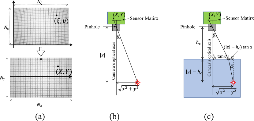
Figure 1: (a) Illustration of the lens distortion (top) and the applied correction together with the coordinate convention (b) Schematic describing the geometry of the camera-luminous point system in air (c) Schematic describing the object-camera system when the object is submerged in a liquid.

2.1 The optics of the object-camera system

We first correct for the lens distortion of the camera, illustrated in the top image of figure 1a, using a sheet of graph paper shown in the bottom image of the same figure. For convenience, we define a pair of auxiliary pixel coordinates $\Xi=\xi-N_{\xi}/2$ and $\Upsilon=\upsilon-N_{\upsilon}/2$ which have their origin at the centre of the image. If the raw camera image has the dimensions of $N_{\xi}\times N_{\upsilon}$ px² an arbitrary luminous point $(\xi,\upsilon)$ has the following corresponding coordinates $(X,Y)$ in the corrected image:

$$X(\Xi,\Upsilon)=\frac{\Xi}{1+K_{1}\left(\Xi^{2}+\Upsilon^{2}\right)}$$ (1)

$$Y(\Xi,\Upsilon)=\frac{\Upsilon}{1+K_{1}\left(\Xi^{2}+\Upsilon^{2}\right)}\,,$$ (2)

where $K_{1}$ is the first radial distortion coefficient of a particular lens, which can be determined by transforming the image until the corrected image is rectilinear (see bottom photograph in fig 1a). The corrected image can be treated as coming from a pinhole camera with the sensor size $N_{X}\times N_{Y}=2X(N_{\xi},0)\times 2Y(0,N_{\upsilon})$, which is larger than the original image if $K_{1}<0$ (see figure 1). The effective pinhole of the lens is the point where all the incoming rays converge and is therefore a convenient choice for the origin of the laboratory’s coordinate system. The position of the pinhole can be determined by photographing a ruler from a known distance, provided the field of view (FOV) angle $\theta_{\rm max}$ of the lens is known. This angle is defined as the angle between the optical axis and the ray arriving at the corner of the image $(X,Y)=(N_{X}/2,N_{Y}/2)$. If the FOV angle is not known, both the position of the pinhole and $\theta_{\rm max}$ can be determined by photographing the ruler multiple times at various known distances. We thus choose the $z$-axis of our coordinate system to be anti-parallel to the optical axis of the camera ($z$ increases in the upward direction) and $x$ and $y$-axes to be, by definition, aligned with the horizontal and vertical axes of the sensor matrix. From this alignment, we write down the first relation between the observed coordinates and the absolute position of the luminous point

$$\frac{x}{y}=\frac{X}{Y}.$$ (3)

The second relation uses the fact that, in a pinhole camera, the rays pass through the pinhole in straight lines, thus the right-angled triangle formed by the pinhole, the luminous point and the optical axis is similar to the triangle between the pinhole, the $(X,Y)$ point and the centre of the sensor matrix, as shown in figure 1b. From this, we calculate the angle $\theta$ between the arriving ray and the optical axis:

$$\tan(\theta)=\frac{\sqrt{X^{2}+Y^{2}}\tan(\theta_{\rm max})}{\sqrt{(N_{X}/2)^{2}+(N_{Y}/2)^{2}}}\,.$$ (4)

Thus, the distance of the luminous point from the optical axis is

$$\sqrt{x^{2}+y^{2}}=|z|\tan{\theta}\,.$$ (5)

If the visualised object is submerged in a liquid of refractive index $n_{f}$, whose surface is $h_{c}$ below the effective pinhole of the camera, (see figure 1), equation 5 becomes

$$\sqrt{x^{2}+y^{2}}=h_{c}\tan{\theta}+(|z|-h_{c})\tan{\alpha}\,,$$ (6)

where, from Snell’s law

$$\alpha=\arcsin{\left(\frac{\sin{\theta}}{n_{f}}\right)}.$$ (7)

2.2 Projection methods

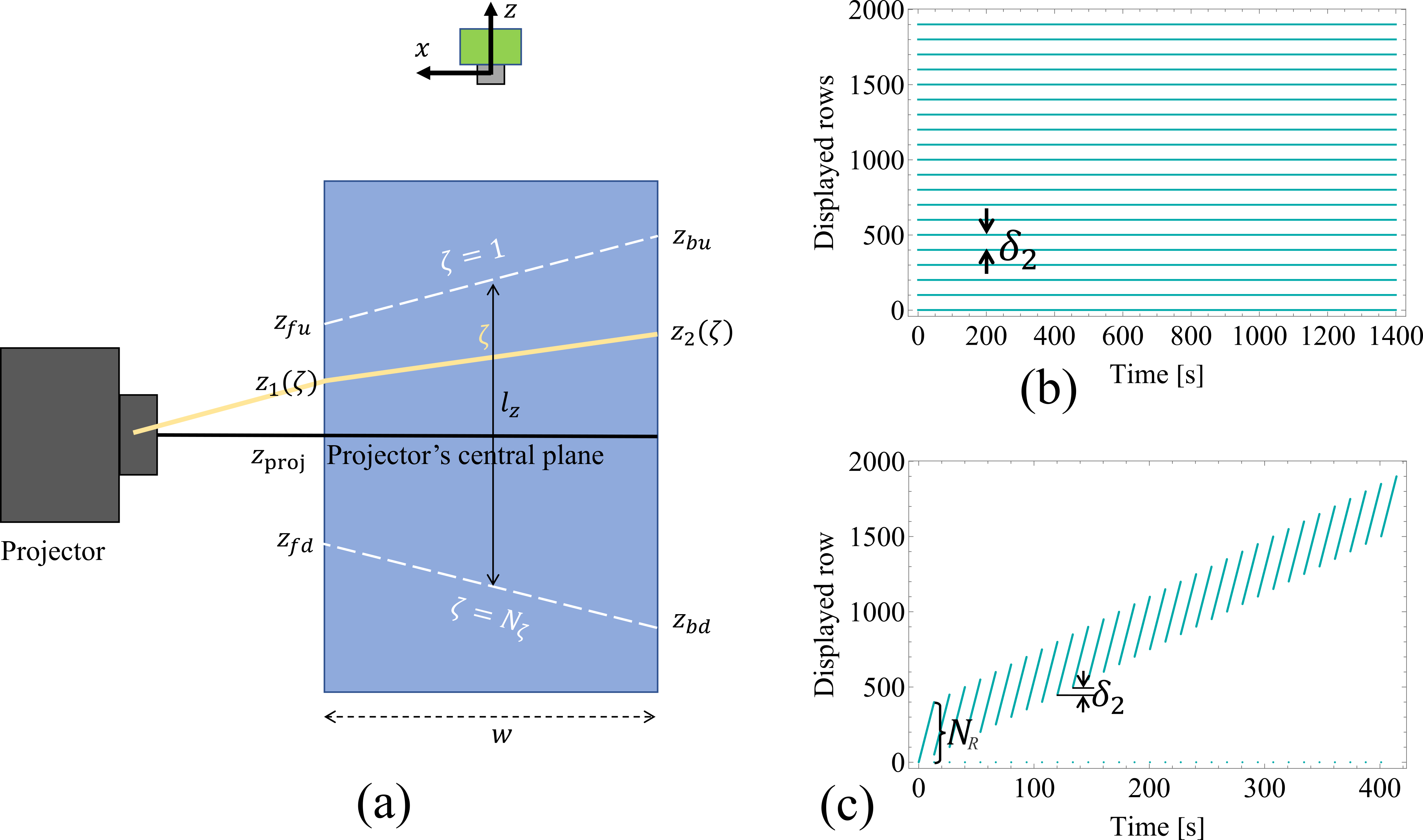
Figure 2: (a) Schematic of the projector system (b) and (c) Time-series of the rows of pixels which are illuminated in static and dynamic modes. In the static mode, (b), multiple rows of pixels spaced $\delta_{2}$ apart are displayed simultaneously. In the dynamic mode, (c), one row of pixels performs a scan in the region of interest of the size of $N_{R}$ after which the projector flashes and the region of interest jumps by $\delta_{2}$ pixels

So far we have constrained the position of a luminous point to a ray of light received by the camera, but to close the system of equations (1)-(7), we need to find the $z$-coordinate of the luminous point. The core principle of our method is that the object is illuminated by a light sheet produced by turning on a single row of pixels in a projector. In this section, we derive an equation $z(x,y,\zeta)$ describing the light sheet cast by the $\zeta^{\rm th}$ row of pixels (see figure 2a). The blue rectangle in figure 2a represents a cuboidal region of interest in which the object is visualised. If the object is submerged in the liquid, it represents the interior of the tank. Our method requires the projector to be aligned horizontally so that the middle light sheet enters and exists this region at the same level. Using the projector in a portrait orientation increases vertical resolution.

It is also important to position and orient the projector such that it doesn’t produce a trapezoidal image in the $yz$ plane ($y$ is out of page in figure 2a). The optics of most commercial projectors are designed with the specific purpose of projecting a rectilinear image onto a screen above the projector in landscape mode, so the beam exits asymmetrically from the lens of the projector. This means that to cast a rectilinear image in the middle of the region of interest when the projector is in portrait orientation, the body of the projector will, counter-intuitively, not align with the axes of the tank.

If the trapezoidal distortion is minimised, the rows of pixels are not tilted in the $y-z$-plane and the planes of light are inclined only in the $x-z$ plane, which is the plane of Figure 2a. The portrait image consists of $N_{\zeta}$ rows of pixels. The first and last rows of pixels cast sheets of light which enter the region at $z_{fu}$ and $z_{fd}$ at the front and exit at the back of the region at $z_{bu}$ and $z_{bd}$. The equations describing the entry point $z_{1}(\zeta)$ and exit point $z_{2}(\zeta)$ of the $\zeta^{\rm th}$ row of pixels are

$$z_{1}(\zeta)=z_{proj}+\left(1-\frac{2\zeta}{N_{\zeta}+1}\right)\left(\frac{z_{fu}-z_{fd}}{2}\right),$$ (8)

$$z_{2}(\zeta)=z_{proj}+\left(1-\frac{2\zeta}{N_{\zeta}+1}\right)\left(\frac{z_{bu}-z_{bd}}{2}\right),$$ (9)

from which the equation for the sheet of light associated with the $\zeta^{\rm th}$ row is

$$z(x,y,\zeta)=\frac{z_{1}(\zeta)+z_{2}(\zeta)}{2}+x\frac{z_{1}(\zeta)-z_{2}(\zeta)}{w}.$$ (10)

Solving equations (1)-(10) gives a unique point $(x,y,z)$ associated with a pixel $(\xi,\upsilon)$ when that point is illuminated by projector’s $\zeta^{\rm th}$ row of pixels. We refer to the solution of these equations as the reconstructor function.

To scan an object with our system, it is necessary that the light sheets move relative to the object. We propose two modes of operating the projector: static, which relies on the visualised object moving through stationary light sheets (displayed simultaneously, see figure 2b) and dynamic, which relies on a light sheet moving from top to bottom at a speed larger than sedimentation speed (see figure 2 for an example time-series of $\zeta(t)$). We will now describe the two modes and provide criteria for choosing the optimal mode for a given scenario.

To ensure that, in the static mode, the falling object is illuminated by at most one light sheet at a given time, the spacing $S$ between the light sheets must be larger than the vertical dimension of the object $s_{z}$. If the vertical dimension of the region of interest is $l_{z}=\frac{z_{fu}+z{b_{u}}-z_{fd}-z_{bd}}{2}$ (see 2a), then the number of scans in the experiment is $l_{z}/S$ and the pixel separation between the lines is $\delta_{2}=SN_{\zeta}/l_{z}$ (see figure 2b). If the average vertical velocity of the object is $\bar{v}_{z}$, then the average time between scans $\bar{T}=S/\bar{v}_{z}$ and the temporal resolution is better the faster the object moves.

One practical issue with the stationary mode is tracking which video frames belong to which scan i.e. we need to split the video into individual scans associated with each light sheet through which the object was passing. This can be done manually by inspecting the video and writing down the timestamps of the frames between each scan, but we propose the following method to automatically detect these frames based on the peaks and troughs of the luminance of the frames. Since the object is not illuminated between the scans, the total brightness of the image is much lower than during the scan. Finding these dark moments enables us to automatically partition the video into the intervals corresponding to separate scans. To do find the dark moments, we first quantify the thermal noise of the camera by capturing several frames of the background, without the object in the system and we calculate the standard deviation of each pixel’s value across the sample. We then average these standard deviations to obtain a mean level of the camera’s thermal noise $\sigma_{t1}$. Then, for each frame in the video taken at time $t$, we calculate the average image of frames between $t-T$ and $t+T/2$, where $T$ is the average time between scans. We divide the current frame by this average and binarize the result with a threshold of $1+3\sigma_{t1}$. This results in the parts of the image corresponding to illuminated portions of the object having a value of 1 and the rest having a value of 0. We count the number of bright pixels and plot the time series of this count across all frames, as shown in figure 3 in blue. We then apply a low-pass filter with a cut-off frequency 30 times smaller than the framerate, shown in orage in figure 3 and apply peak detection to find the minima corresponding to frames between scans. These minima split our video into individual scans.

The main strengths of the static method are: (a) its independence from the projector’s refresh rate, which translates to (b) the lack of need to synchronize the camera with the projector, which allows simple and direct control of the temporal resolution of each scan through camera’s framerate, as well as (c) the lack of need to synchronise the projector with the motion of the object which makes the method applicable to any arbitrarily large velocity and velocity variation of the particle, which translates to (d) the simplicity of setting up the experiment without prior information about the particle’s motion. The main downside of this method is its inapplicability to stationary objects and the poor temporal resolution when the object is translating very slowly.

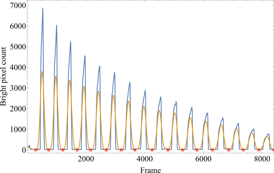
Figure 3: Blue line: The time series of the total brightness of a binarized image as the object passes through stationary planes of light. Orange line: A low-pass filtered version of the time-series, whose minima (red points) are the basis for splitting the video into separate scans in the static mode.

In the dynamic mode, the projector is operated by a video of a descending row of pixels. To save time between scans, the scan is limited to a region of interest of $N_{R}$ rows, and the line moves $\delta_{1}$ pixels every frame (see figure 2c). After the scan is completed, the projector flashes with a fully white frame to signify the end of the scan and the scan repeats with its region of interest being lower by $\delta_{2}$ pixels to keep up with the object. The framerate of the video matches the framerate $f$ of the camera, which must be an integer divisor of the nominal framerate of the projector. The flashes, which are $N_{R}+1$ frames apart, allow verifying whether the camera has captured all the frames or not.

We now proceed to derive several expressions useful for making the optimal choice of the parameters $N_{R},\delta_{1},\delta_{2},f,l_{z}$ based on the object’s vertical dimension $s_{z}$, vertical velocity $v_{z}(t)$, whose average is $\bar{v}_{z}$ and the desired temporal resolution represented by the time between scans $T$. For simplicity, we will assume that $N_{R}\gg 1$ so that $N_{R}\approx N_{R}+1$. The scanning speed of the projector is

$$v_{s}=\frac{\delta_{1}l_{z}}{N_{\zeta}}f\,,$$ (11)

which must be strictly larger than $v_{z}$ or the dynamic mode cannot be used.

The most optimal size of the region of interest is the smallest necessary to encompass the size of the sheet $s_{z}$ plus the amount it translates during the scan. If the sheet translates steadily with velocity $\bar{v}_{z}$, the time it takes to scan the sheet is $s_{z}/(v_{s}-\bar{v}_{z})$. If the sheet translates with a variable velocity $v(t)$, the region of interest must be enlarged by a sufficient margin $m$ so that the sheet does not escape the region of interest, and thus the time between scans is given by:

$$T=\frac{s_{z}+m}{v_{s}-\bar{v}_{z}}\approx\frac{(s_{z}+m)N_{\zeta}}{\delta_{1}l_{z}f}\,,$$ (12)

Where the last approximation holds for $v_{s}\gg\bar{v}_{z}$. Thus, if the sheet changes its shape rapidly, requiring frequent scans, $T$ can be decreased by increasing the product $\delta_{1}l_{z}f$. Intuitively, for a shape-shifting or reorienting particle, $T$ must be at least an order of magnitude shorter than the shortest of the timescales associated with the change of shape or reorientation, which typically translates to reorientation rates less than $\sim 18\degree$ between scans and to the rate of motion of boundary points relative to the centroid of the sheet less than $\sim 0.1a$, where $a$ is the lengthscale of the sheet. Once $T$ is selected, the appropriate value of $N_{R}$ is

$$N_{R}=T\delta_{1}f=\left(\frac{s_{z}+m}{v_{s}-\bar{v}_{z}}\right)\delta_{1}f\approx\frac{(s_{z}+m)N_{\zeta}}{l_{z}}\,.$$ (13)

where the last inequality, again, holds when $v_{s}\gg\bar{v}_{z}$.

To find the optimal choice of $\delta_{2}$ we need to consider the speed at which the region of interest follows the object

$$v_{f}=\frac{\delta_{2}l_{z}}{N_{\zeta}T},$$ (14)

and equate it to the average falling speed $\bar{v}_{z}$. Substituting $T$ from equation (12) we get

$$\delta_{2}=\frac{N_{\zeta}(s_{z}+m)}{l_{z}}\frac{v_{z}}{v_{s}-\bar{v}_{z}}\approx\frac{N_{\zeta}^{2}(s_{z}+m)\bar{v}_{z}}{l_{z}^{2}\delta_{1}f}$$ (15)

where, as before, the final approximation applies when $v_{s}\gg v_{z}$. Finally, we note the following condition for when it is better to use the dynamic mode as opposed to the static mode:

$$T<\frac{s_{z}}{\bar{v}_{z}}\Leftrightarrow\bar{v}_{z}<\frac{s_{z}(v_{s}-\bar{v_{z}})}{s_{z}+m}\,.$$ (16)

This means, the dynamic mode is more suitable for slowly-moving objects with small velocity variation so as not to require a large choice of the margin $m$.

2.3 Image processing and data extraction

Once the experiment is finished, the frames captured by the camera must be processed to address three challenges: (a) the biased and noisy signal from the camera sensor; (b) the background illumination of the object caused by the fact that projectors have finite contrast i.e. even the black pixels emit some light; (c) the inevitable presence of specks of dust which are also illuminated by the projector.

We first calibrate the camera sensor using the flat-field correction which involves subtracting the electronic bias of the camera and compensating for the varying pixel sensitivities. The bias field is determined by taking a series of images in darkness (e.g with a cap on the lens) while the pixel sensitivities are determined by taking a set of ’flat’ frames i.e. frames where the incoming signal is uniform, such as when photographing a stack of light diffusers. The average level of brightness of a flat frame $\langle{\rm flat}-{\rm bias}\rangle$ should ideally be of the order of 0.5. Thus, to compensate for varying pixel biases and sensitivities, the corrected image is computed by the formula:

$${\rm calibrated}=({\rm input}-{\rm bias})\frac{\langle{\rm flat}-{\rm bias}\rangle}{{\rm flat}-{\rm bias}}\,.$$ (17)

Finally, the sensors of digital cameras always have some level of thermal noise $\sigma_{t1}$ which can be calculated by taking a standard deviation of the set of flat images. From now on, we assume all images are calibrated and their level of thermal noise is known.

Because some specks of dust can be highly reflective they may appear brighter than the illuminated object itself, so prior to the rest of the analysis we multiply every image by a constant $A$ chosen such that the typical brightness of the light scattered by the object is close to 1 and we clip the pixel values above 1 to 1. This way the specs of dust are no brighter than the signal we want to observe. To remove the background illumination of the object coming from the ambient light of the projector and the environment, we subtract from each frame the average image of the scan to which this frame belongs. Then, for each scan, we stack thus background-subtracted images into a 3D image containing $N_{\xi}\times N_{\upsilon}\times N_{R}$ voxels. Then, we perform a 3D convolution with a small Gaussian kernel of 1.5-voxel standard deviation which reduces the level of noise approximately tenfold to $\sigma_{t2}=\sim 0.1A\sigma_{t1}$. We binarize this 3D image with a threshold of $3\sigma_{t2}$ (see figure 4a for an example image after applying this threshold) which means that only statistically-significant signal remains bright which includes the sheet and the visible dust. We call this 3D image $I_{1}$.

To remove the specks of dust present in $I_{1}$ we must estimate the density field of the image and use the fact that on intermediate length scales (between the size of the specks and the size of the object), the density of white voxels corresponding to the object is higher than the density of the voxels corresponding to the specks of dust. We, therefore, compute two voxel-counting convolutions $I_{2}$ and $I_{3}$ with two different cubical kernel sizes $s_{2}$ and $s_{3}$, respectively, which use uniform kernels whose entries have a constant value of 1. This way, the output of each convolution counts the number of white voxels in $I_{1}$ contained in the cubes of dimension $s_{2}\times s_{2}\times s_{2}$ and $s_{3}\times s_{3}\times s_{3}$, respectively. The $I_{2}$ image is strongly blurred and uses the size $s_{2}$ much larger than the largest specks of dust while being an order of magnitude smaller than the visualised object. Relative to the size of the kernel, the dust is point-like, while the surface or volume of the object is one-, two-, or three-dimensional. Thus, the appropriate threshold for removing dust and preserving the object is $\sim s_{2}^{d}$, where $d$ is the object’s dimensionality. This, however, preserves the specks of dust in the vicinity of the object’s surface. To remove these, a finer convolution $I_{3}$ of $I_{1}$ is applied with a kernel size $s_{3}$ by no more than one order of magnitude larger than the typical size of the speck of dust in $I_{1}$. The appropriate threshold is again $\sim s_{3}^{d}$. To compute the cleaned result we take the product $I_{4}=I_{1}I_{2}I_{3}$, an example of which is shown in figure 4b.

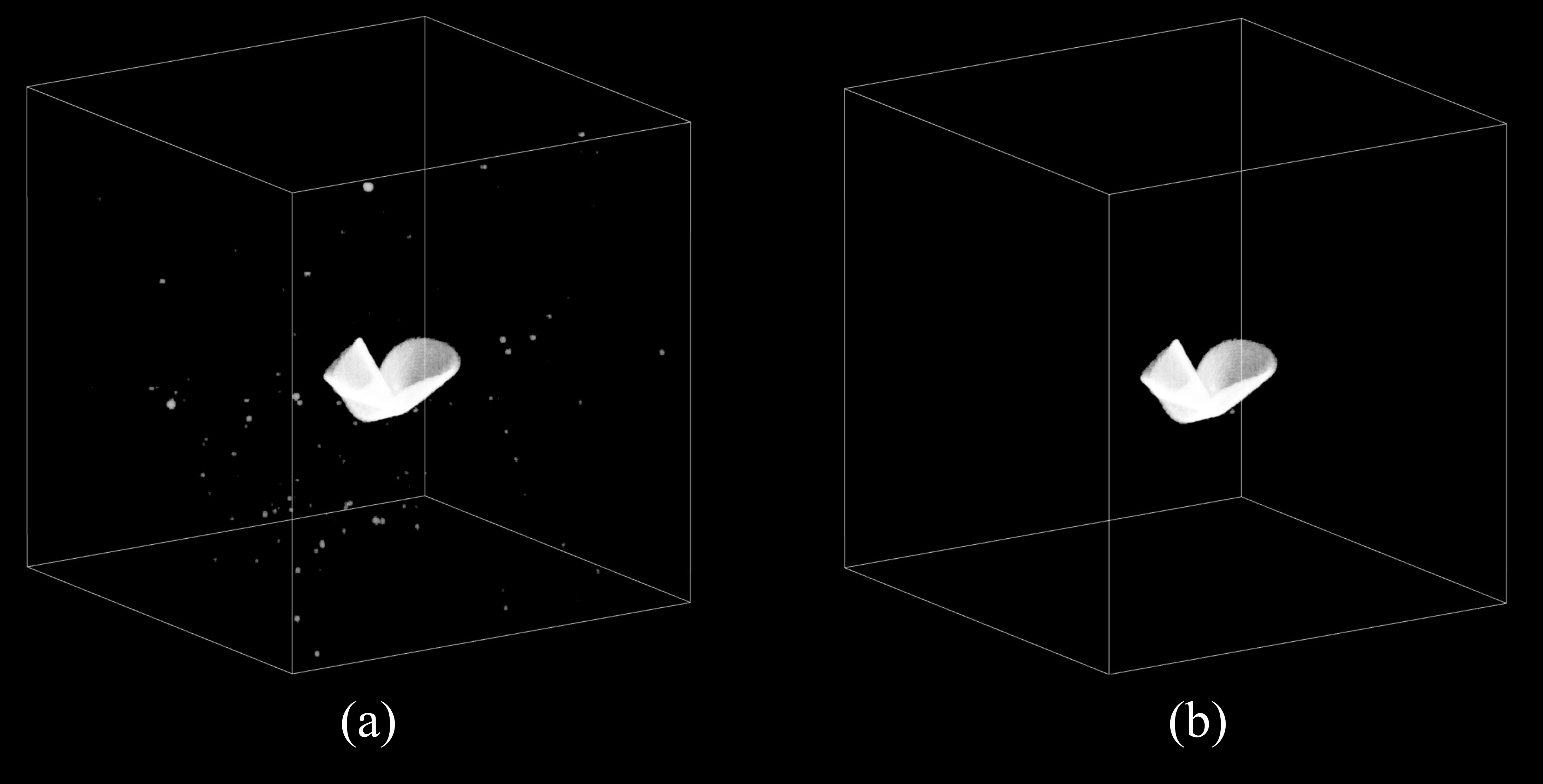
Figure 4: (a) An example 3D image of a sheet scanned in the dynamic mode after the first convolution, before the removal of the specks of dust. (b) The cleaned dataset after removing the specks of dust

The data is now ready for reconstruction. We apply the reconstructor function to the coordinates $(\xi,\upsilon,\zeta)$ of every bright voxel in $I_{4}$ and obtain the (x,y,z) coordinates of that luminous voxel. By also including the time at which each voxel was scanned, we generate a series of four-dimensional clouds of points $\{(x_{ij},y_{ij},z_{ij},t_{ij})\}_{\rm raw}$ where $i$ labels individual scans and $j$ labels individual points in the $i^{\rm th}$ scan. We refer to this dataset as the hypercloud.

2.4 Rolling shutter

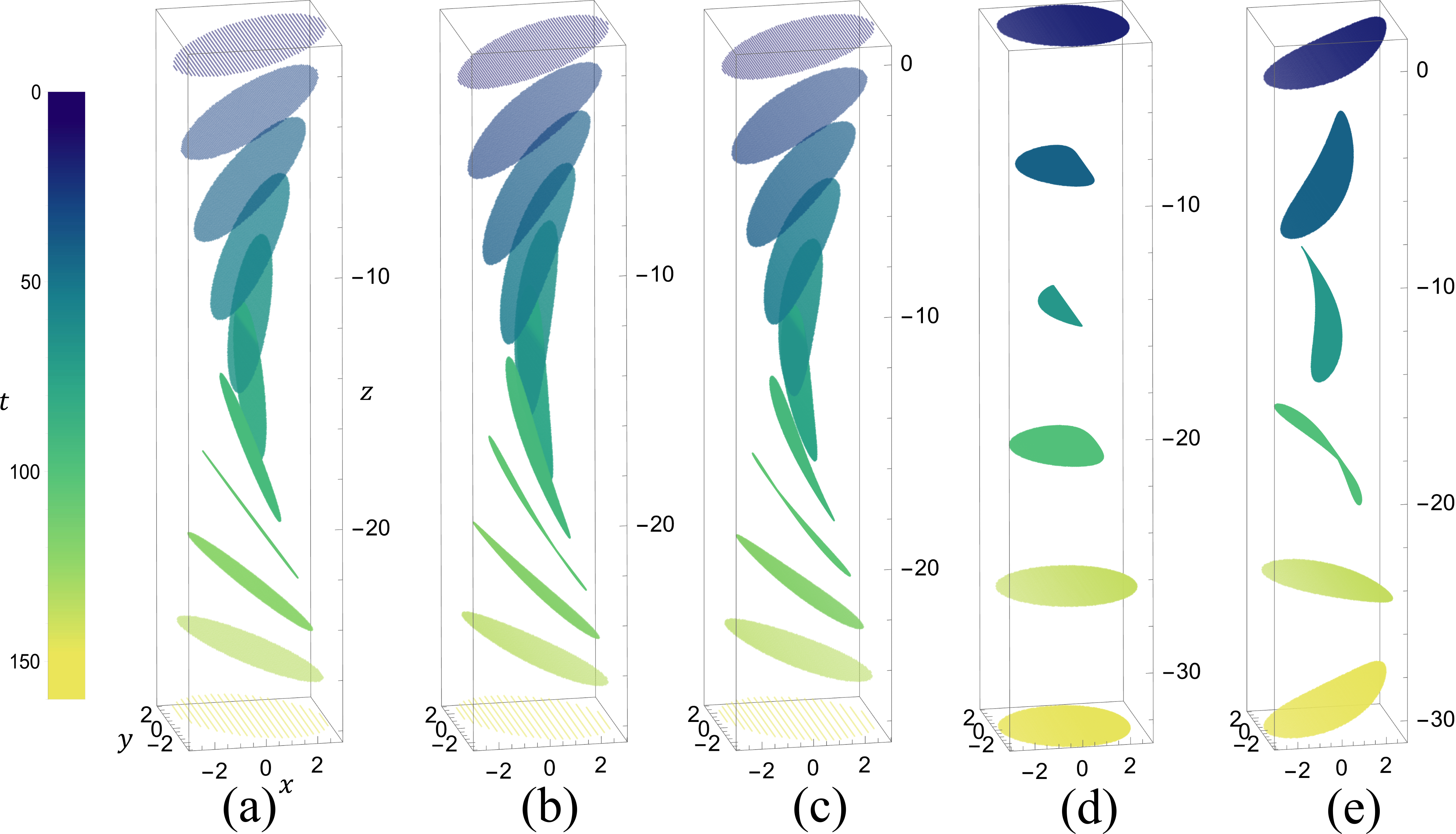
Figure 5: A simulated spatial components of the hypercloud for a translating and rotating synthetic disk scanned at two different speeds. (a) At a slow scanning speed, rolling-shutter distortions are present in the form of elongated and curved appearance. (b) At ten times higher speed, the disk these distortions are negligible.

A nuanced consequence follows from the fact that the scanning speed is finite: the spatial components $(x,y,z)$ of the hypercloud exhibit a rolling-shutter distortion caused by the fact that the upper and lower portions of the sheet are scanned at different moments in time. In the dynamic mode, the upper portions are scanned before the lower portions, whereas in the dynamic mode the lower portions are scanned first. Figure 5 illustrates these distortions on a simulated dataset of a sedimenting and reorienting flat disk of radius $R=3$ cm, with downward velocity of $2$ mm/s, and angular velocity $1.3\degree$/s in the y-direction, starting from the initial inclination of $5\degree$. In subfigure (a), the simulated scanner casts $N_{\zeta}=400$ consecutive horizontal lines spaced $0.3$/,mm apart. The framerate is $300$ fps and $\delta_{1}=1$, so the scanning velocity is $90$ mm/s. In subfigure (b), on the other hand, the framerate is $30$ fps, so the scanning speed is $9$ mm/s. Comparing the two images, we see that, in the dynamic mode, the rolling-shutter distortion manifests itself in two ways. First, the fact that the disk translates during the scan causes the disk in subfigure (b) to be elongated in the z-direction relative to subfigure (a), especially when the disk is near-vertical. The second feature is caused by the fact that the disk rotates during a scan which causes the output in (b) to be curved.

A more drastic distortion appears in the stationary mode shown in subfigure (d). All spatial data associated with one scan is degenerated to the 2D plane of the stationary light sheet involved in that scan. In this mode, all of the three-dimensional information about the sheet is encoded in the time component of the dataset.

It is important to note that these distortions are not errors of the hypercloud dataset. However, they make it necessary for the surface reconstruction method to involve fitting a full 4D model which takes temporal information into account. It is also important to note that when comparing the spatial part of the hypercloud against the output of thus fitted model for a particular moment in time, the fit will appear of poor quality: the distorted data will not perfectly match the non-distorted reconstruction. To alleviate some of these plotting problems, it is possible to compensate for the translational distortion of the dataset by computing the velocity $\boldsymbol{v}(t)$ of the centre of mass of the sheet using finite differences between scans. Assuming the velocity varies slowly on the timescale of a scan, an auxiliary dataset ${x_{ij}^{\prime},y_{ij}^{\prime},z_{ij}^{\prime}}$ can be constructed:

$$x_{ij}^{\prime} =x_{ij}+v_{x}(t_{ij}-t_{is})$$ (18)

$$y_{ij}^{\prime} =y_{ij}+v_{y}(t_{ij}-t_{is})$$ (19)

$$z_{ij}^{\prime} =z_{ij}+v_{z}(t_{ij}-t_{is})$$ (20)

$$t_{ij}^{\prime} =t_{is}$$ (21)

where $t_{is}$ is the time at the start of the $i^{\rm th}$ scan. The auxiliary datasets for the data corresponding to subfigure (b) is shown in figure (c). We see that the vertical elongation is reduced and matches that of figure (a). The auxiliary dataset for the static mode is shown in (e). We see that the size and approximate orientation is recovered, but the nonlinear distortion is in the opposite direction caused by the fact that the lower portions of the disk are scanned first.

3 Shape reconstruction

3.1 Fitting parametric surface

Given a hypercloud of $N_{p}$ data points $(x_{ij},y_{ij},z_{ij},t_{ij})$, where $i$ labels individual scans and $j$ labels individual point in the scan, we want to fit a time-evolving surface represented parametrically i.e. represented by a set of bounded functions $\hat{x}(u,v,\tau)$, $\hat{y}(u,v,\tau)$ and $\hat{z}(u,v,\tau)$, where $u$ and $v$ are surface parameters and $\tau$ is the time parameter. However, the functional form of this parametric representation is not known a priori, and the data points are disordered i.e. we don’t know the mapping from the direct $(x,y,z,t)$ space into $(u,v,\tau)$ parameter space. In particular, we don’t know which of the points in the hypercloud are at the boundary of the sheet. The only order the hypercloud has is in time, making the mapping between $t$ and $\tau$ trivial, by setting $\tau=t$. Therefore, we need to find two mappings: the first one identifies a data point $(x_{ij},y_{ij},z_{ij},t_{ij})$ with the parameters $(u_{ij},v_{ij},t_{ij})$ and the second one which parametrises the surface, mapping the $(u,v,t)$-space onto $(\hat{x},\hat{y},\hat{z})$ in a way that minimises the Mean Euclidean Distance (TED) between the fitted surface and the data points:

$${\rm MED}=\frac{1}{N_{p}}\sum_{ij}\sqrt{(x_{ij}-\hat{x}_{ij})^{2}+(y_{ij}-\hat{y}_{ij})^{2}+(z_{ij}-\hat{z}_{ij})^{2}}\,,$$ (22)

but also ignores the noise i.e. the mapping does not overfit the points, but is smooth enough to follow the shape of the surface. We propose guessing both mappings with an autoencoder neural network [16] which is a fitting procedure designed to parametrise higher-dimensional noisy data with a lower-dimensional manifold. Neural networks typically have a large number ($10^{4}-10^{12}$) of optimisable parameters making them suitable to approximate any arbitrary function of unknown form to any desired level of detail. They also provide an easy way to ensure that the resulting parametrisation is smooth so that useful quantities such as normals and curvatures can be computed.

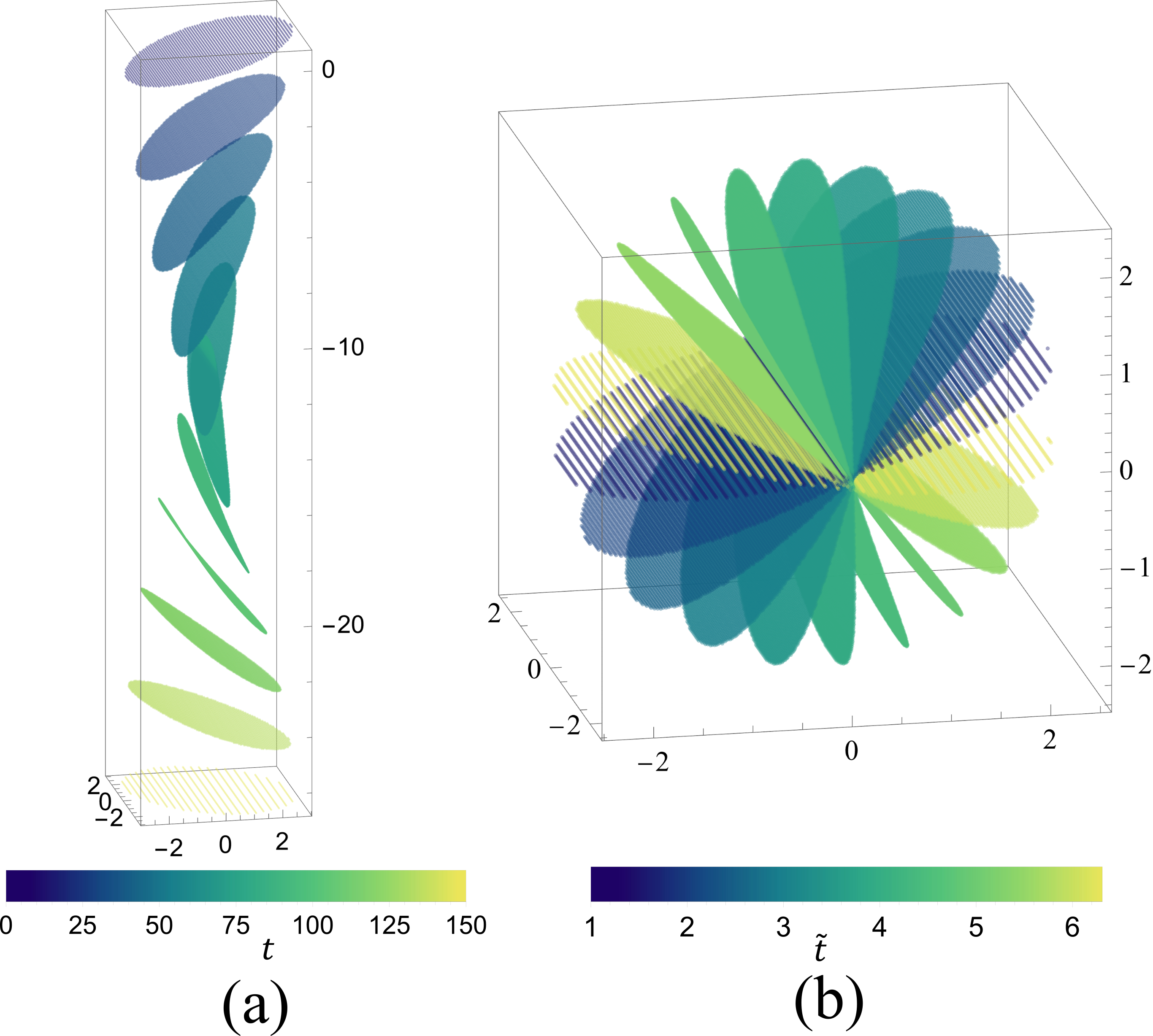
Figure 6: (a) An example hypercloud of input $(x,y,z,t)$ points (b) The dataset after normalization following equations (23)-(12)

Before we introduce the details of this fitting procedure, we should discuss the preparation of the dataset. For reasons detailed in reference [17], both accuracy and the speed of convergence of machine-learning algorithms are often significantly hindered if the inputs are highly correlated or unnormalised. If, for example, our surface translates by a large distance, say, in the z-direction (see figure 6 for illustration), the input’s $z$-component will be highly correlated to the time component. Thus, it is beneficial for convergence to approximate the translational motion of the sheet $\bar{x}(t),\bar{y}(t)$ and $\bar{z}(t)$ and remove it from the dataset. This translational motion can be computed by calculating for each scan $i$ the average $\bar{x}_{i}$, $\bar{y}_{i}$, $\bar{z}_{i}$ and $\bar{t}_{i})$ and fitting, for example, a first or second-order polynomial to each component’s time-series. The removal of the translational motion not only decorrelates the input but also helps to ensure that the large-scale features of the trajectory do not overshadow (in terms of their contribution to the TED) the small-scale features of the shape of the sheet. Thus created dataset should then be normalised by rescaling it homothetically by dividing each component by $\sigma=(\sigma_{x}+\sigma_{y}+\sigma_{z})/3$, where $\sigma_{x},\sigma_{y},\sigma_{z}$ are the respective standard deviations of all values $x_{ij},y_{ij},z_{ij}$ in the hypercloud. Thus, we propose the following set of transformations:

$$\tilde{x}_{ij} =\frac{x_{ij}-\bar{x}(t_{ij})}{\sigma}$$ (23)

$$\tilde{y}_{ij} =\frac{y_{ij}-\bar{y}(t_{ij})}{\sigma}$$ (24)

$$\tilde{z}_{ij} =\frac{z_{ij}-\bar{z}(t_{ij})}{\sigma}\,.$$ (25)

The exact optimal choice of rescaled time $\tilde{t}$ is, however, data-dependent but several useful guidelines can be provided. Because we want our model to ignore the high-frequency noise of the data, this also imposes a limitation in resolving high-frequency detail in the time domain. Therefore, the usual consideration of normalising the time domain to a size of the order of unity must be balanced against the fact that the model converges better when the sheet does not evolve too rapidly i.e. when the average rates of change $|d\tilde{x}/d\tilde{t}|$, $|d\tilde{y}/d\tilde{t}|$, $|d\tilde{z}/d\tilde{t}|$ of material points of the sheet do not exceed the order of unity. If the time between scans $T$ is selected as advised in the discussion of equation (12), these conditions are satisfied when time is rescaled by $T$. However, such rescaling means that exactly one scan populates a unit of time $\tilde{t}$ which, in the course of trial and error we found was too sparse causing significant errors in the interpolation between scans. Moreover, we noticed that, for no obvious reason, most of the autoencoders we tested generate discontinuities in the vicinity of $\tilde{t}=0$, so we heuristically offset the time-domain to all $\tilde{t}_{ij}>1$. Thus, we propose the following transformation:

$$\tilde{t}_{ij}=\frac{t_{ij}}{2T}+1\,.$$ (26)

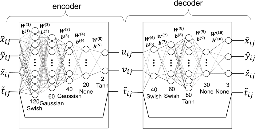
Figure 7: Caption

The autoencoder (see figure 7) is effectively composed of two neural neural networks connected back-to-back: the encoder, which finds the mapping from the higher dimensional space in which data is distributed to a lower-dimensional latent space, and the decoder, which finds the mapping from the lower-dimensional latent space back to the higher-dimensional direct space. Unlike the simplest neural networks which are used to learn labelled data sets $(\rm input_{i},target_{i})$, where each input has an externally provided target (e.g. the MNIST dataset contains images of hand-written digits and human-labelled "ground truth" answers [18]), the autoencoder’s task is to predict its own input as accurately as possible, under the dimensionality-reduction constraint. The main premise of the autoencoder is that the most optimal way to fit a lower-dimensional manifold to higher-dimensional noisy data is to eliminate the noise.

It is important to emphasise a further subtle difference between our use of an autoencoder and canonical forms of machine learning. In most cases, such as image classification, neural networks learn a diverse set of examples to the end of applying them to previously unseen examples. For that purpose, the neural network’s performance is evaluated on a set of validation data not encountered previously by the network. By contrast, our method focuses on a single experiment, with the objective of memorising the hypercloud dataset as accurately as possible under the constraints of the dimension-reduction task. Thus, there is no benefit in using a validation set.

The details of the architecture of the autoencoder we propose are shown in Figure 7. The flow of information is from left to right. The autoencoder can be treated as a stack of two modules: the encoder and the decoder. Because the mapping of time is trivial, the time output is the same as the time input in both modules. The spatial mappings, on the other hand, are determined using two neural networks.

Each of the neural networks is a stack of five neural layers. Each layer passes its output as an input to the next layer. Mathematically, an $n^{\rm th}$ neural layer produces an output vector $\boldsymbol{X}^{(n)}$ which is calculated by applying a tunable weight matrix $\boldsymbol{W}^{(n)}$ to the input vector $\boldsymbol{X}^{(n-1)}$, adding a tunable bias vector $\boldsymbol{b}^{(n)}$ and applying an activation function $f^{(n)}$ to each element of thus produced vector:

$$\boldsymbol{X}^{(n)}=f^{(n)}(\boldsymbol{W}^{(n)}\boldsymbol{X}^{(n-1)}+\boldsymbol{b}^{(n)})\,\,.$$ (27)

The number of columns of the weight matrix $\boldsymbol{W}^{(n)}$ is the dimension of $\boldsymbol{X}^{(n-1)}$ and the number of rows is the chosen number of neurons for this layer i.e. the dimension of $\boldsymbol{X}^{(n)}$. If the input vector is $\boldsymbol{X}^{(0)}$, then the functional form of the encoder’s neural network is

$$\boldsymbol{X}_{(5)}=f^{(5)}\left(\boldsymbol{W}^{(5)}f^{(4)}\left(\boldsymbol{W}^{(4)}f^{(3)}\left(\boldsymbol{W}^{(3)}f^{(2)}\left(\boldsymbol{W}^{(2)}f^{(1)}\left(\boldsymbol{W}^{(1)}\boldsymbol{X}^{(0)}+\boldsymbol{b}^{(1)}\right)+\boldsymbol{b}^{(2)}\right)+\boldsymbol{b}^{(3)}\right)+\boldsymbol{b}^{(4)}\right)+\boldsymbol{b}^{(5)}\right)\,,$$ (28)

which is a length-2 vector mapping a $(\tilde{x}_{ij},\tilde{y}_{ij},\tilde{z}_{ij},\tilde{t}_{ij})$ point onto a $(u_{ij},v_{ij})$ latent point. Appending to this output the $\tilde{t}_{ij}$ point we get the full output of the encoder $\boldsymbol{X}_{\rm enc}$ which is then fed to the decoder, whose neural network has the following functional form:

$$\boldsymbol{X}^{(10)}=f^{(10)}\left(\boldsymbol{W}^{(10)}f^{(9)}\left(\boldsymbol{W}^{(9)}f^{(8)}\left(\boldsymbol{W}^{(8)}f^{(7)}\left(\boldsymbol{W}^{(7)}f^{(6)}\left(\boldsymbol{W}^{(6)}\boldsymbol{X}_{\rm enc}+\boldsymbol{b}^{(6)}\right)+\boldsymbol{b}^{(7)}\right)+\boldsymbol{b}^{(8)}\right)+\boldsymbol{b}^{(9)}\right)+\boldsymbol{b}^{(10)}\right)\,.$$ (29)

To ensure the smoothness of the fitted manifold, only smooth activation functions were considered in the design of the network. These include the ${\rm Swish}(x)=x/(1+e^{-x})$, the ${\rm Gaussian}(x)=e^{-x^{2}}$, and the $\tanh$ function. The selection of the activation functions and the number of neurons in each layer was done in a process of trial and error which does not guarantee the most optimal configuration, but we found the performance to be robust for a wide range of datasets, as discussed in sections 4 and 5. The total number of adjustable parameters in the encoder is $N_{e}=11162$ and in the decoder is $N_{d}=10023$, which, relatively speaking, is a very lightweight neural network. Below each neural layer in figure 7, we list the number of neurons and the activation functions for that layer. We write "None" for the layers which do not have a nonlinear activation function and, instead, perform only an affine transformation of the input. This is mathematically equivalent to applying $f(x)=x$. To ensure the latent space is bounded, we use $\tanh$ as encoder’s last activation function.

We now proceed to describe the training of the neural network which is a process in which the weights and biases of all neural layers are found. As with every optimisation process, we start with an initial guess, called the initialisation of the neural network. Typically, the biases are all zero, while the weights are initialised using a variety of methods. We found the best initialisation for our encoder’s weights is obtained by using Kaiming’s method [19], while the weights of the decoder are suitably initialised using identity initialisation [20], which, ensures that the decoder initially parametrises an approximately flat sheet. Training of a neural network is a process which seeks to find the values of the tunable parameters which minimise the loss function, which in our case is MED (see equation (22). As is the case in all gradient-based optimisation methods, this requires us to compute the gradient of the loss function with respect to every weight and bias. If traditional non-linear optimisation methods were used, the calculation of this gradient would be prohibitively slow, requiring $N_{p}\times(N_{e}+N_{d})\approx N_{p}\times 2\times 10^{4}$ evaluations of the neural network, each of which takes about a millisecond. One way to speed up the process is to split the dataset into smaller batches and approximate the gradient by calculating it relative to each batch. This means that if the batch size is ${B}$, the network is updated $N_{p}/B$ times before it has seen all the data points. The iterations associated with each cycle of $N_{p}/B$ iterations is called an epoch. Using a low $B$ increases the number of batches per epoch, at the cost of the accuracy in gradient approximation. However, this alone would still be prohibitively slow, taking about 20 seconds per example. The advantage of using a neural network, as opposed to general nonlinear fitting, comes from the fact that the gradients can be calculated through backprogapagtion without the need to evaluate the network for each parameter. Equation 27 can be rewritten as

$$\boldsymbol{Z}^{(n)} =\boldsymbol{W}^{(n)}\boldsymbol{X}^{(n-1)}+\boldsymbol{b}^{(n)}$$ (30)

$$\boldsymbol{X}^{(n)} =f^{(n)}(\boldsymbol{Z}^{(n)})\,.$$ (31)

The gradients are given by the following recurrence [17]

$$\frac{\partial C}{\partial\boldsymbol{Z}^{(n)}} =f^{\prime}(\boldsymbol{Z}^{(n)})\frac{\partial C}{\partial\boldsymbol{X}^{(n)}}$$ (32)

$$\frac{\partial C}{\partial\boldsymbol{X}^{(n-1)}} =(\boldsymbol{W}^{(n)})^{T}\frac{\partial C}{\partial\boldsymbol{Z}^{(n)}}$$ (33)

$$\frac{\partial C}{\partial\boldsymbol{W}^{(n)}} =\frac{\partial C}{\partial\boldsymbol{Z}^{(n)}}\boldsymbol{X}^{(n-1)}$$ (34)

$$\frac{\partial C}{\partial\boldsymbol{b}^{(n)}} =\frac{\partial C}{\partial Z^{(n)}}\,.$$ (35)

This means, that if we know $\frac{\partial C}{\partial\boldsymbol{X}^{(n)}}$, we can calculate $\frac{\partial C}{\partial\boldsymbol{Z}^{(n)}}$ from which we can calculate the gradients of the $n^{\rm th}$ layer as well as $\frac{\partial C}{\partial\boldsymbol{X}^{(n-1)}}$ needed to calculate the gradients of the previous layer and so on all the way to the first layer. This means only the gradients of the loss function with respect to the output layer need to be evaluated and the remaining gradients are obtained very quickly. The network is ready for optimisation.

We recommend training the network with a batch size of $B=512$ using the ADAM optimizer [21]. We perform training in three stages: 1.5 million iterations (updates after each batch) with the step size (also called learning rate) of $10^{-3}$, followed by 0.8 million iterations with the step size of $10^{-4}$ and 0.1 million iterations with a step size of $10^{-5}$. The initial larger step size speeds up the learning of the large-scale structure of the dataset, after which the following stages gradually fine-tune the model. We test the training on a laptop with an NVIDIA GeForce 1050Ti graphics card, and the training takes approximately 2.5 hours ($\sim 260$ iterations per second). The VRAM memory allocated to the training process on a dataset of $N_{p}=7\times 10^{6}$ data points is 1.3 gigabytes, which means the training can be performed on virtually any graphics card available on the market.

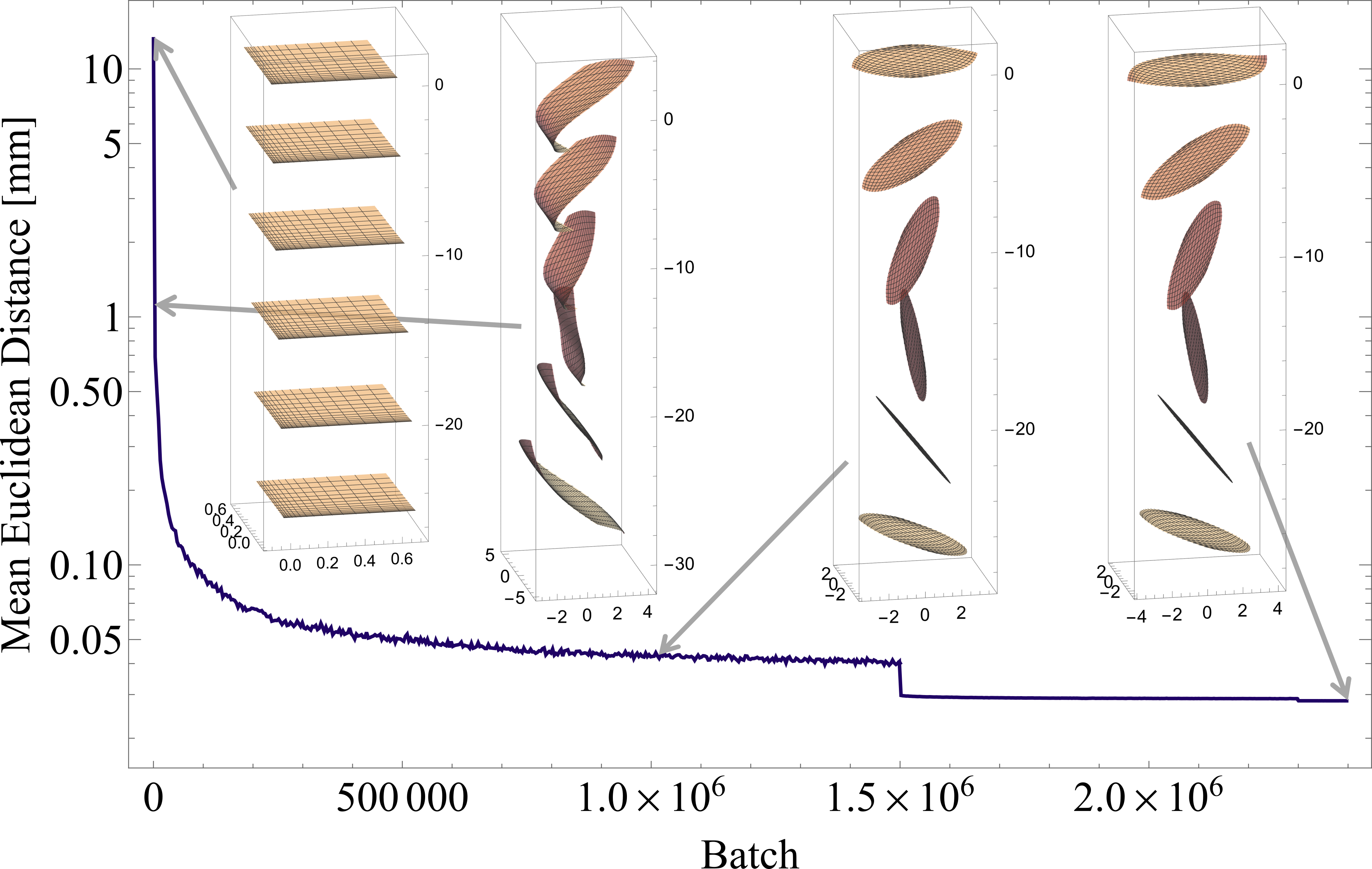
Figure 8: An example learning curve of the autoencoder showing the three stages of learning with decreasing learning rates. Insets show slices of parametrisation at selected stages of learning where $u$ and $v$ vary from $-1$ to $1$. First inset: Initial state prior to learning (0 batches). Second inset: after 1 epoch (2832 batches). Third inset: after 1.4M batches. Fourth inset: after 2.4M batches, when the training is finished

We track the progress of the training of the autoencoder by saving a copy of the network after the completion of each epoch and calculating the MED associated with it. An example learning curve showing how MED changed as training progressed is shown in figure 8. In the first stage of 1.5 million batches the neural network eventually plateaus and progress is slow. When the second stage begins, the model is fine-tuned and a noticeable dip in MED occurs. After the second stage is complete, the last stage of 100 thousand batches fine-tunes it again, but the drop in MED is significantly less pronounced demonstrating that the model has essentially converged. We can extract the decoder in real-time from the saved copies of the network to preview the current reconstructed shape. Recall that the decoder is the parametrisation of the surface in the scaled coordinates, so by inverting the scaling equations (23)-(26) we recover the sought-for functions $x(u,v,t)$, $y(u,v,t)$, $z(u,v,t)$. Plotting the functions over a square domain of $u$ and $v$ ranging from $-1$ to $1$, we can preview the parametrised manifold in real-time. Three time-slices of the manifold at various stages of the training process are shown in the insets of figure 8. The first inset shows the state prior to learning, a flat horizontal surface. After the first epoch, the shape has substantial error, but eventually, the correct shape is found and the fine-tuning process indeed makes only very small adjustments to the shape, as can be seen in the last two insets. It is important to note, however, that some portions of thus plotted manifold are extrapolations, which is due to the fact that we naively sampled the whole domain of the latent coordinates $u$ and $v$. The method for finding the boundary between the fitted and extrapolated regions is introduced in the next section. After the training is complete and the parametrisation is found, we can calculate all useful local quantities such as normal vectors, principal curvatures and principal directions of curvature, which is detailed in Appendix A.

3.2 Determination of the boundary

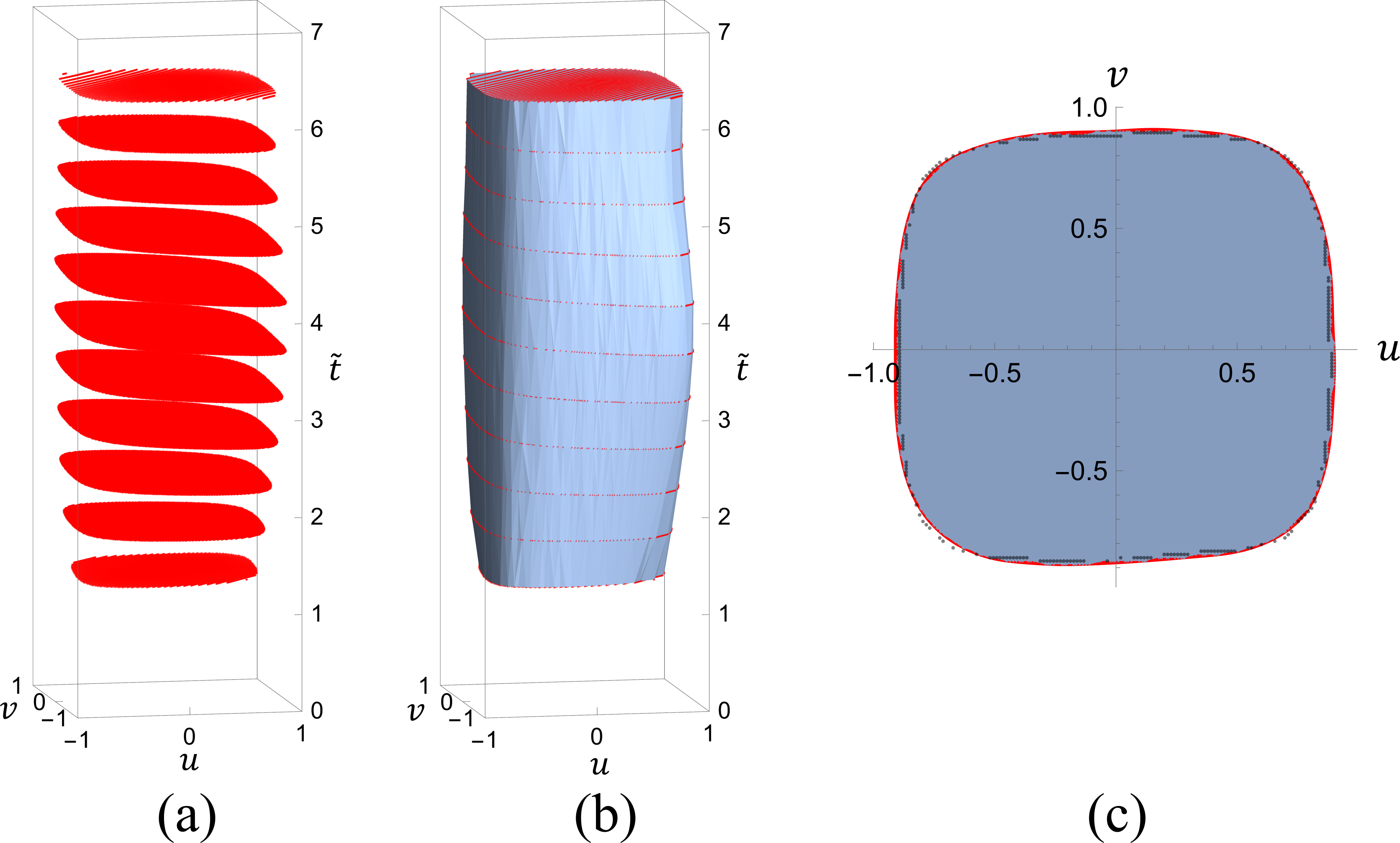
Figure 9: (a) The latent cloud of points produced by applying the encoder to the hupercloud. The points form surfaces associated with each scan. (b) The alpha shape used to interpolate the boundary of the sheet between the latent surfaces. (c) An example time-slice of the alpha shape. Black points lie closest to the boundary of the alpha shape, this boundary is jagged. Red: a smoothed version of the boundary obtained by constructing a B-spline from the black points. This red line demarkates the boundary of the sheet in the latent space

The final step in reconstructing the sheet is determining its boundary in the latent space $(u,v,t)$. For this purpose, we apply the encoder to the hypercloud to generate the latent cloud, whose points lie on surfaces belonging to each scan as shown in Figure 9a. These surfaces are not horizontal in the time dimension because the sheet is not scanned instantaneously, as discussed in section 2.4. This means we need to interpolate the boundary between the scans. An additional challenge is posed by the fact that, while these latent surfaces have the same topology as the sheet, $u$ and $v$ do not correspond, in general, to the material coordinates of the sheet. For example, a circular sheet may be mapped by the encoder onto a non-convex region. To interpolate between these latent surfaces, we encompass the dataset with a tight-fitting 3D mesh, in the following way: First, we temporarily scale down the time $\tilde{t}$ of the latent cloud by a factor of 10, so that the latent surfaces are a distance of 0.05 apart. Then we find the alpha complex of the data with ball radius $\alpha\simeq 0.15$. The definition of the alpha complex of a 3-dimensional point cloud $S$ is a subcomplex of Delaunay triangulation of $S$ which retains only those simplexes whose circumsphere is empty (i.e. does not contain any other points of $S$) and whose radius is smaller than $\alpha$ [22]. In our context, it is crucial that $\alpha$ be larger than the spacing between the latent surfaces but small enough to follow the concavities of the latent surfaces. Once the alpha complex is found, its time dimension is rescaled back by a factor of 10 to its original normalised time scale as shown in Figure 9b. Moreover, we are only interested in its boundary (called the alpha shape), which saves memory and shortens the time it takes to evaluate whether a point (u,v,t) lies inside or outside this boundary.

As can be seen in Figure 9b, the resulting alpha shape has a jagged surface. The size of these kinks is necessarily smaller than $\alpha$. Therefore, for a selected time-slice $\tilde{t}$, we discretize the $u-v$-space into a square $N_{\rm latent}\times N_{\rm latent}$ lattice and find the lattice points in the interior of the alpha shape the outermost of which are shown in black in Figure 9c. We propose smoothing the boundary with a B-Spline function of the order $N_{\rm spline}\sim N_{\rm bound}/2$, where $N_{\rm bound}$ is the number of these outermost points. This smoothed boundary should be enlarged by a factor of $1+2/N_{\rm latent}$ to compensate for the fact that the points to which it was fitted were already inside the accepted interior. Thus smoothed boundary is marked in red in Figure 9c with its interior filled in blue. Having selected the set of $(u,v)$ points which belong to the sheet at a chosen time $t$, we can feed them into the decoder and into the functions calculating the normals, principal curvatures, principal directions and surface elements and get a full reconstruction of the sheet.

4 Validation on synthetic datasets

We measure the accuracy of the autoencoder on two synthetic datasets: an origami zig-zag (see Figure 10 and a surface made to resemble undulating wrinkles (see Figure 11). The zig-zag dataset is inspired by the recent interest in origami structures as well as the fact that such a zig-zag also forms in nature [23]. The zig-zag is a piecewise linear function with curvature singularities, so fitting a smooth manifold must necessarily under-resolve the sharp folds. This provides a useful benchmark of the autoencoder’s ability to resolve short-wavelength details. The undulating surface, on the other hand, is a useful test of the autoencoder’s ability to reconstruct strongly wrinkled surfaces which cannot be represented as single-valued functions. The geometry is also suitable for testing the accuracy relative to varying levels of noise since, at large noise levels, the data from distinct portions of the sheet would overlap, confusing the encoder.

4.1 Origami zig-zag

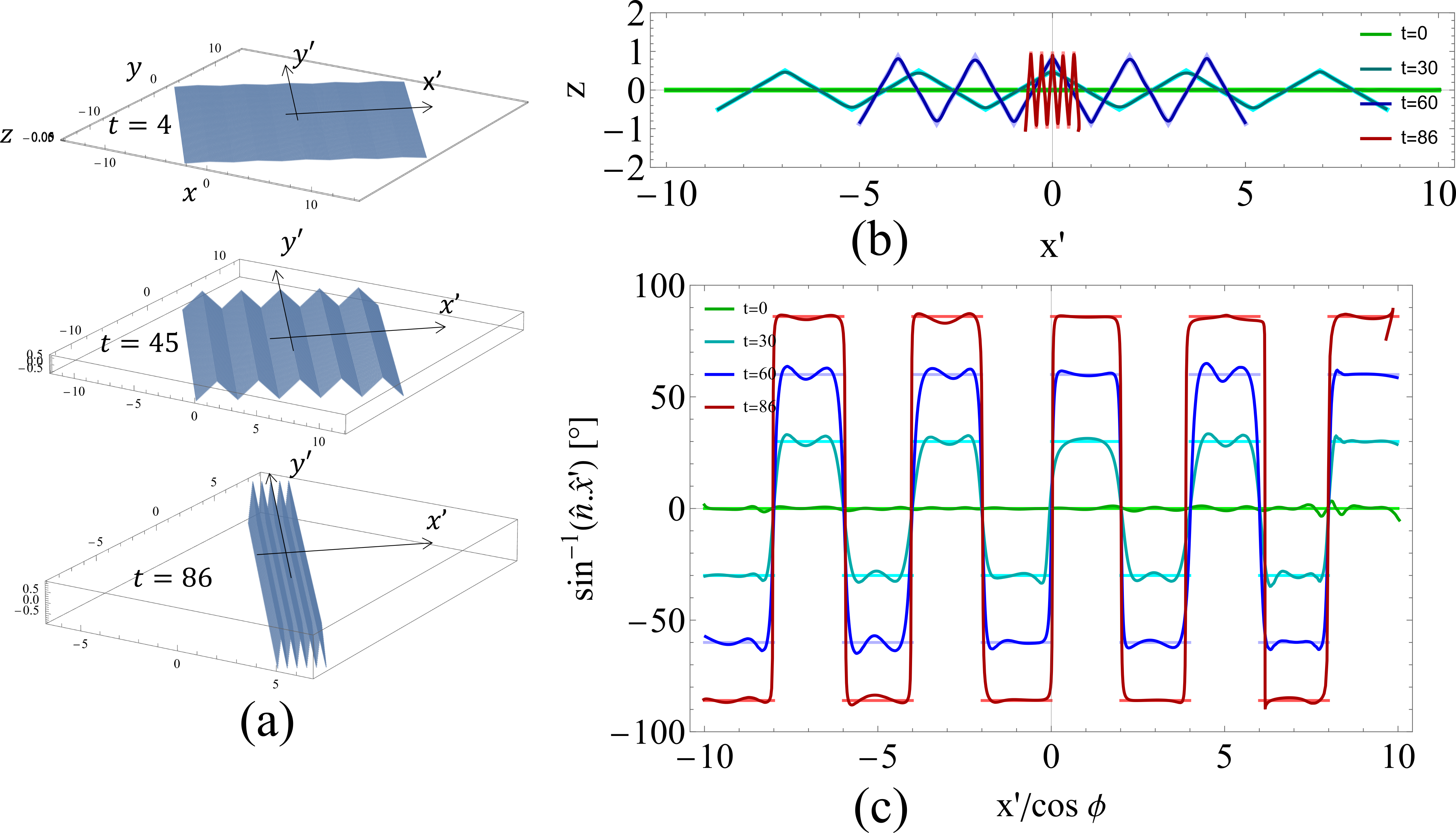
Figure 10: (a) Three selected time slices of the folding zig-zag dataset. (b) The $y^{\prime}=0$ cross-section of the reconstructed surface (dark thin lines) plotted on top of the ground truth for reference (bright thick lines). The reconstruction rounds the sharp corners. (c) The local inclination profile of the reconstructed surface (dark thin lines) plotted against the ground truth (bright thick lines).

The zig-zag’s shape at $t=0$ is a flat $20\times 20$ square, and as time progresses, the ten segments of the zig-zag fold: the angle $\phi$ between the vertical and the normal vector of any segment changes in time as $\phi=\degree t$, where t ranges from 0 to 89 in steps of 1. There are $4\times 10^{4}$ equally distributed points in each time slice. The zig-zag’s $x^{\prime}$-axis is rotated relative to the $x$-axis by an arbitrarily chosen angle of $37\degree$. We train the autoencoder.

The final mean euclidean distance between the reconstruction and the target was $2.4\times 10^{-4}$ of the side length of the square. Figure 10b shows $y^{\prime}=0$ cross-sections through the output (dark thin lines) on the background of the target shape of the zig-zag (bright thicker lines) for four selected time-slices: $t=0$, $t=30$, $t=60$ and $t=86$. The autoencoder has successfully reconstructed all ten segments of the zig-zag, irrespective of the slopes. It is visible that the largest discrepancy is at the folds, which appear rounded in the output. Figure 10c shows the inclination of the same output plotted against a rescaled coordinate $x^{\prime}/\cos\phi$.

At the centres of the segments, the inclination matches the target inclination, shown in corresponding brighter lines, to within $4\degree$. The zig-zag is flat along the $y^{\prime}$ axis, so the target radius of curvature in that direction is infinite. In the reconstructed zig-zag, the typical radius of curvature in this direction is $2500$, two orders of magnitude larger than the side length of the sheet 20.

4.2 Undulating wrinkles

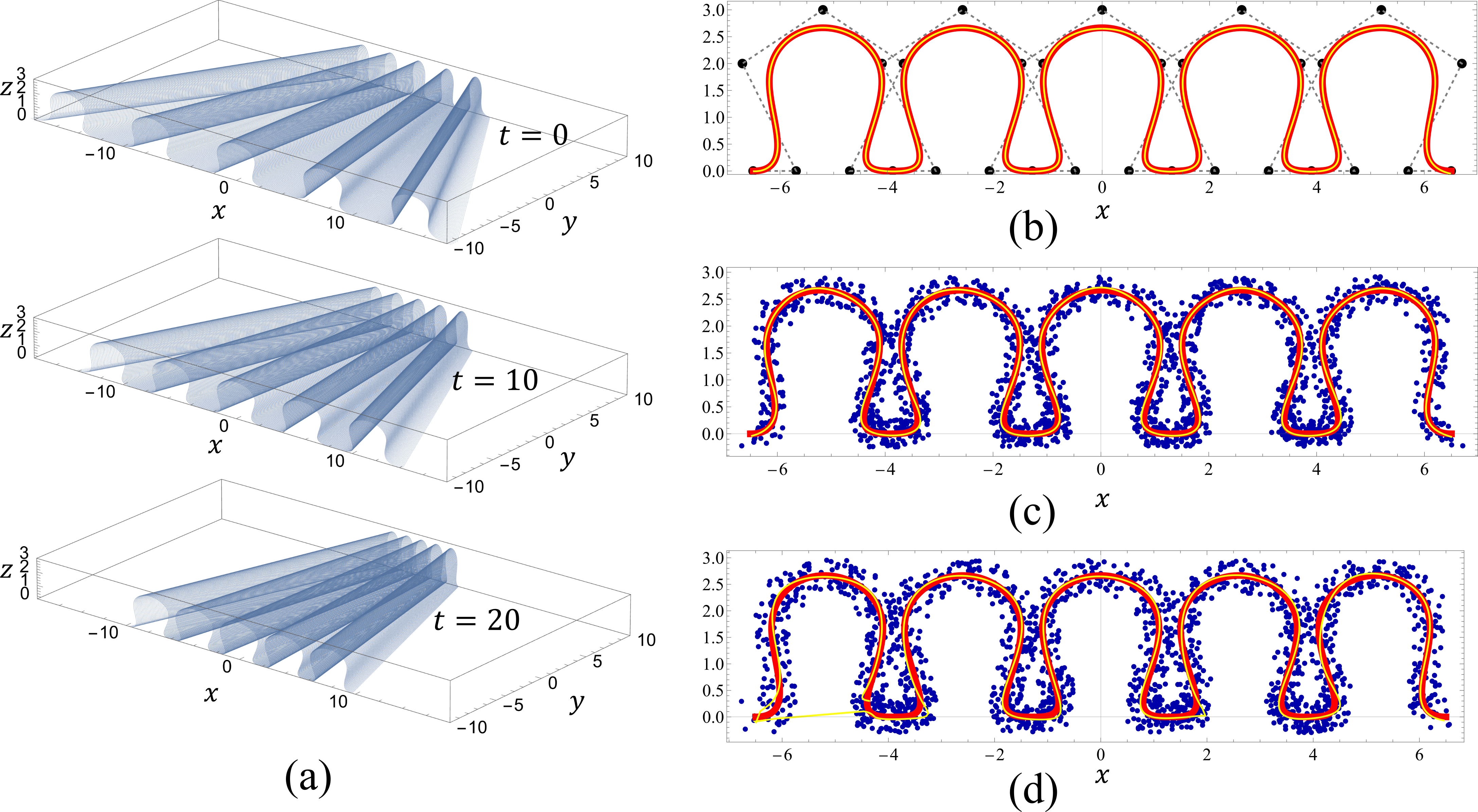
Figure 11: (a) Synthetic point clouds for three time-slices of the undulating surface. (b) Red line: a $y=0$, $t=20$ cross-section of the wrinkled surface, which is a B-spline function produced using the black points as control points in the order indicated with dashed line. Thin yellow line: a $y=0$, $t=20$ cross-section of the reconstructed surface. (c) Blue points: a slice of the noisy input data with $\lambda=0.25$, thin yellow line: a slice of the reconstructed surface and thick red line: the ground truth (unperturbed surface). (d) At $\lambda=0.3$ the reconstruction fails to find the correct ordering of points and thus creates a bridge seen in the bottom left of the image

The undulating wrinkled surface, whose first ($t=0$), middle ($t=10$) and last ($t=20$) time-slices are shown in figure 11a, was synthesised using B-spline functions with control points moving inwardly with time, as described in detail in appendix B. The control points of the last time slice and the resulting spline are shown in Figure 11b. The variation in $y$ is done by horizontally compressing the spline of each time slice by substituting the $x$-components with $(1-0.05y)x$. This linear dependence preserves the developability of the surface, making the wrinkles d-cones pointing radially towards a common apex at $(x,y)=(0,20)$. The size of the sheet in the $y$-direction is 20, whereas in the x-direction is variable. A cloud of 400k points is produced for each of the integer values of $t$. We train the autoencoder, and inspect the results with a particular focus on the last time slice, in which the wrinkles are separated by only $0.4$ at $y=0$.

The mean euclidean distance between the target and a central cross-section of the output of the autoencoder for $t=20$ was $4.2\times 10^{-3}$ which is $2.1\times 10^{-4}$ of the $y$-dimension of the sheet. Figure 11b shows the output as a thin yellow line on top of the target represented by the thicker red line.

We also repeated the training for a variety of noisy datasets, where each point was perturbed in every spatial dimension by a random value between $-\lambda$ and $+\lambda$. Here, we report the results for two selected values of $\lambda$: $0.25$ and $0.3$. Figures 11(c) and (d), show the $t=20$ and $y=0$ slices for each of these datasets respectively. In each figure, the dark blue points are the $z-x$-projection of the (perturbed) input datasets for this slice, and the thick red line is the slice of the unperturbed dataset (the ground truth), shown for reference. The thin yellow line is the corresponding slice of the reconstruction. We observe that the algorithm successfully reconstructs the surface at the noise levels up to $0.25$, which is approximately the borderline level at which points belonging to materially distant parts of the sheet touch. At this level, the average deviation, over the whole manifold, between the reconstructed surface and the reference surface is $1.9\times 10^{-2}$, which is $1.9\times 10^{-3}$ of the $y$-dimension of the sheet. The reconstruction of the dataset with the 0.3 noise level suffers from a bridge at the bottom-left part of Figure 11d. The encoder failed at correctly identifying the order in which the surface should pass through the points. The surface begins at $(x,y)=(-4.4,0.3)$ cm, wraps around the first wrinkle in the anti-clockwise direction before making a bridge to the second wrinkle. This additional bridge results in a larger total area of the reconstructed manifold, as well as significant curvature artefacts on either side of the bridge.

5 Experimental validation

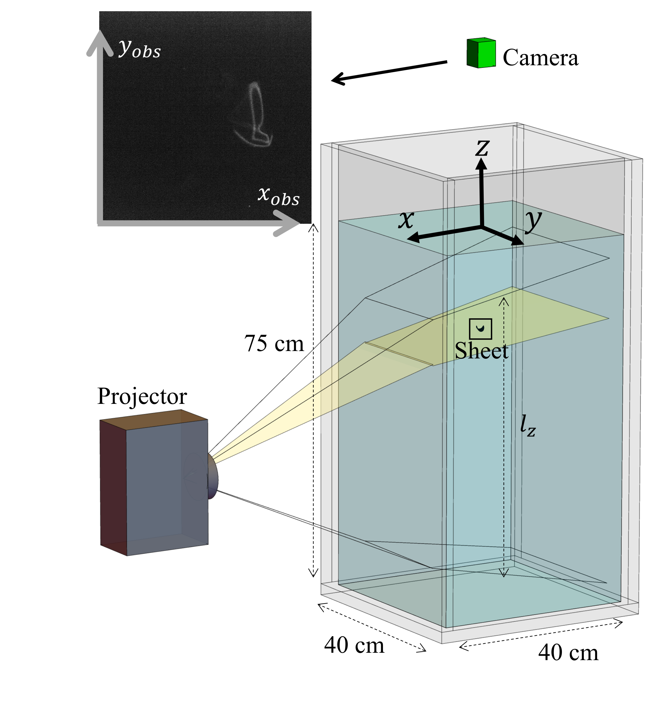
Figure 12: Schematic of the experimental set-up (to scale) operated in a dynamic mode, with a single plane of light shining through a sheet. The contours of the transparent planes show the first and last rows of pixels of the projector. Inset: an example image captured by the top-view camera during a scan of a crumpled sheet.

We validate our method on a particular experimental example of a PDMS sheet of radius $R=29.75\pm 0.16$ mm, and 100 μm thickness falling in a $40\times 40\times 90~{}{\rm cm}^{3}$ tank filled to a level of 75 cm with 1000 cSt silicone oil, as shown in Figure 12. We use an Optoma HD143X projector whose longer edge has a resolution of 1920 pixels placed such that in the middle of the tank, $l_{z}=56.8$ cm. Thus, the absolute vertical resolution is $l_{z}/1920=295$ μm. The projector is operated in a dynamic mode with $\delta_{1}=1$ and $\delta_{2}=40$ at the framerate of $f=30$ fps. We used a 5 Mpx (2560x2048) JAI GO-5000M-USB camera with a Kowa LM16HC lens with $K_{1}=-13.5\times 10^{-9}$ and $\theta_{\rm max}=44.3\degree$ and placed it 59.5 cm above the surface of the liquid. The example raw image captured by the camera of a crumpled sheet is shown in the inset of figure 12.

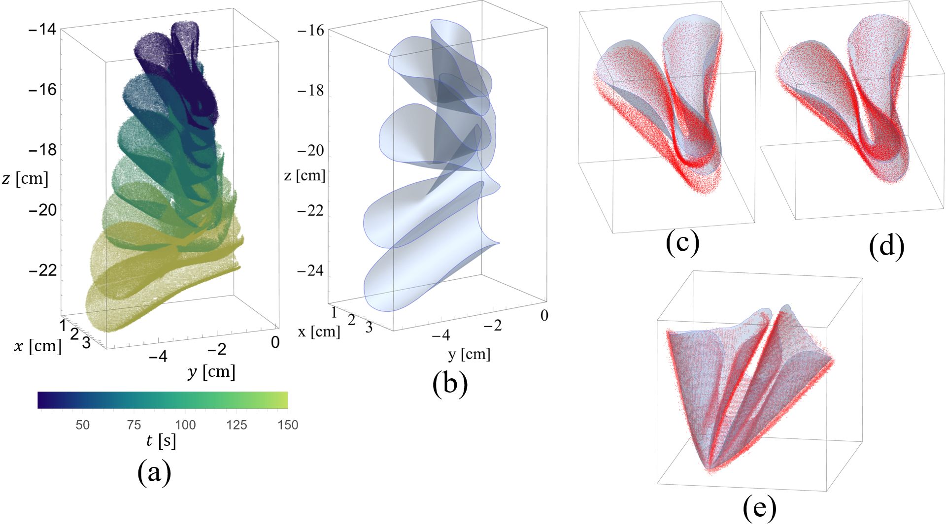
Figure 13: (a) A 4D hypercloud of points as extracted from an experiment in which an initially crumpled sheet unfolded. The points are colour-coded by time. (b) Four selected time-slices of the reconstructed surface of the sheet (c) The of the reconstructed surface and the hypercloud data suffering from the rolling-shutter. (d) The comparison with the auxiliary dataset where translational rolling-shutter was compensated (e) the same as in (d), but with the view onto the tip of the crumple

The experiment was initialised in a crumpled state (folded in four) and during the experiment, the sheet uncrumpled, as shown in the plot of the spatial component of the hypercloud in Figure 13a and the series of reconstructed shapes shown in figures 13b. The autoencoder successfully identified the configuration of the surface despite the fact that some areas, which materially belong to the opposite sides of the circle, find themselves in close proximity in 3D. Figure 13c shows the overlay of the spatial component of the second scan of the hypercloud, which happened during the interval between $2<\tilde{t}<3$ and its reconstruction for $\tilde{t}=2$. As discussed in 2.4, the point cloud is vertically stretched due to the rolling shutter effect, which was compensated for the purposes of comparison according to equations (18)-(21) and the result is shown from the front and from the back is in figure 13(d) and (e), respectively. The reconstruction fits the data very well, including the localised feature of the tip of the crumple. The effective radius across all time-slices, as calculated from its area, has a mean $R_{\rm eff}=\sqrt{A/\pi}=29.65$ mm, and fluctuates across time slices with standard deviation of 0.4 mm.

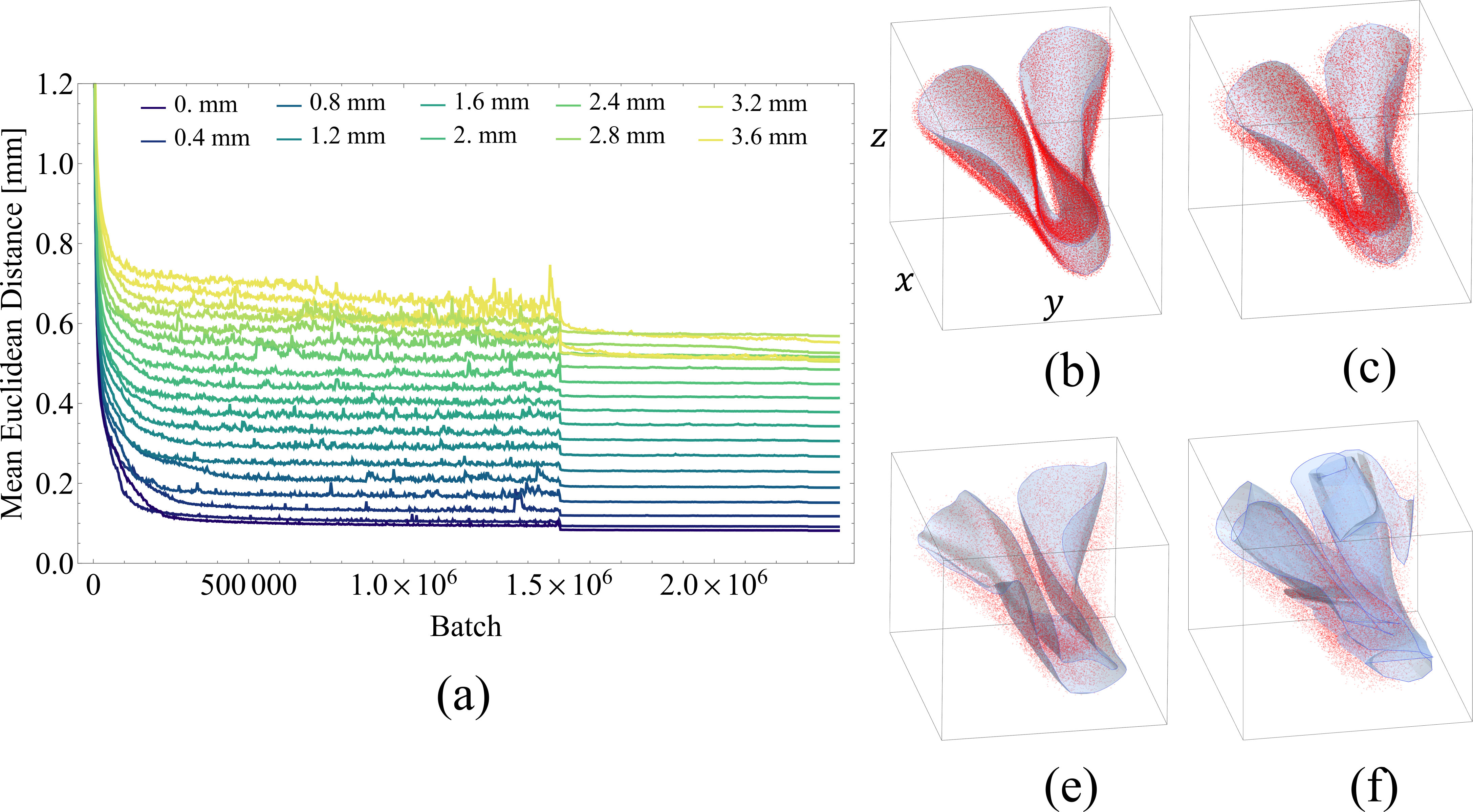
Figure 14: (a) Learning curves for the unwrinkling sheet with various levels of added noise. The sudden drops are a result of training switching to a lower learning rate. (b)-(e) Point clouds of the second scan of the sheet with artificially added noise and their reconstructed shapes: (b) $\lambda=0$, successful reconstruction (c) $\lambda=1.4$ mm, where the points belonging to materially distant regions are touching, successful reconstruction, (d) $\lambda=2.6$ mm, reconstruction has curvature artefacts, but correct large-scale configuration (e)$\lambda=3.4$ mm, failed reconstruction

To determine the limits of successful reconstruction, we artificially added different levels of noise by perturbing each point in the hypercloud by a random value between $-\lambda$ and $\lambda$ in the $x$ and $y$ dimensions, to imitate a scenario where the thickness of the scattered light, as observed by the camera is larger. The learning curves for different values of noise are shown in Figure 14(a). Each curve has three stages corresponding to the three consecutively smaller values of the learning curve mentioned in section 3.1. For $0.4<\lambda<3$ mm, we observe a linear dependance between the final value of MED and $\lambda$. The intercept at $\lambda=0$ of this linear trend is ${\rm MED}=40\pm 2$ μm, which is below the vertical resolution of the projector and 10 μm below the half-thickness of the sheet’s material, indicating that the image thresholding has accepted only a thin portion of the observed luminous lines. However, at $\lambda=0$, the final value of MED is $82{\rm\mu m}$ which is a factor of 2 higher than the intercept of the linear trend. This discrepancy is $7\times 10^{-3}$ of the diameter of the sheet, consistent with our tests on synthetic datasets described in section 4, indicating that the autoencoder reached the limit of its resolution. At $\lambda>3$ mm, the learning curves are qualitatively different: the values break away from the monotonic trend and the learning has not reached a plateau in the second stage. This suggests that the dataset is so diffuse that the shape is irreconstructible.

To visualise the effect noise has on the reconstruction, we show the perturbed datasets and thei respective reconstructions in figures 14(b)-(e) for $\lambda$ equal to 0, 1.4 mm, 2.6 mm and 3.4 mm, respectively. At $\lambda=1.4$ mm the reconstruction approximately preserves developability. At $\lambda=2.8$ mm the surface has prominent curvature artefacts, but the overall shape has a correct large-scale configuration. At $\lambda=3.6$ mm the reconstruction failed to capture even the large-scale features, contains extra folds and even self-intersections. Similarly to the case of undulating wrinkles, the noise level at which the reconstruction begins to exhibit bridging happens at $\lambda=1.8$ mm and corresponds approximately to a scenario where point clouds from materially distant portions of the sheet begin to overlap. For $\lambda>1.8$ mm, the significant overlap between different portions of the point cloud prohibits the encoder from correctly identifying which data points belong to which parts of the sheet. This misidentification, in turn, distorts the parameterisation. Eventually, at large levels of noise ($\lambda>3$ mm), successful reconstruction is impossible.

Another effect that the noise has on the reconstruction is the Gaussian curvature of the sheet. Figure 15(a) shows the average Gaussian curvature of the sheet in its final, uncrumpled U-shaped state as a function of $\lambda$. In this state, the target Gaussian curvature is zero, since the sheet is developable everywhere, so it will have zero extrinsic curvature in a "flat" direction, parallel to the spine of the U. We set an upper bound on the desired curvature in the "flat" direction to be one order of magnitude lower than $1/R$ i.e. such that in non-dimensional terms $\tilde{\kappa}_{2}=\kappa_{2}R<0.1$.

Since the other principal curvature in the direction perpendicular to the spine of the sheet is $\kappa_{1}=60$ m^-1, we find that the upper bound of the Gaussian curvature is $\sim 200$ m^-2, which we plot as the dashed line in Figure 15a. Thus, we conclude that the reconstruction meets our criterion for $\lambda<1.1$ mm. For $\lambda$ between 1.8 mm and 3 mm, which is the regime where curvature artefacts are prominent, Gaussian curvature fluctuates significantly, as would be expected from random curvature artefacts. For $\lambda>3$ mm, Gaussian curvature increses rapidly, which is consistent with our observations from the learning curves and figure 14 that reconstruction fails.

Finally, we examine the effect the noise has on the reconstructed effective radius of the sheet, which is shown as points in figure 15b. The error bars in the figure show the standard deviation of the area across the time dimension. For reference, we show the solid line corresponding to the measured radius of the sheet with the thickness corresponding to the measurement uncertainty. For $\lambda<1.4$ mm, the results are consistent. As $\lambda$ increases, the reconstructed area also increases. Beyond $\lambda=2.8$ mm, the reconstructed radius is significantly overestimated and shows large temporal fluctuations.

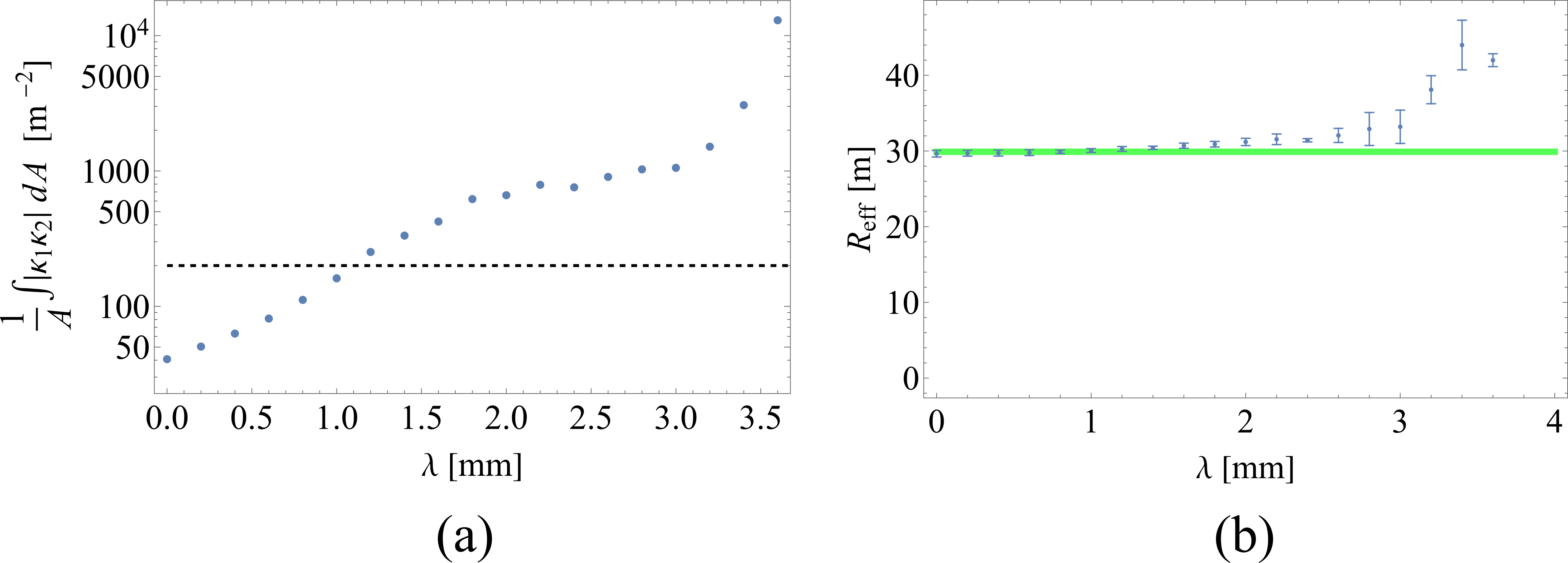
Figure 15: (a) The dependence of Gaussian curvature of the reconstructed sheet on the level of added noise $\lambda$, measured at the final time-slice when the sheet is fully-uncrumpled and U-bent. The dashed line is the level below which the sheet can be approximated as developable. (b) Blue points: the reconstructed effective radius of the sheet as a function of the level of added noise $\lambda$. The error bars are the standard deviation across different time-slices. The solid line is the measured radius of the sheet and its thickness corresponds to the mearsurement uncertainty.

6 Conclusions

The visualisation method we propose is a relatively cheap and non-intrusive way of observing three-dimensional objects. Using a 5 Mpx camera and a commercial Full-HD procjector, we are able to perform 10 gigavoxel scans. The absolute resolution of the system is limited primarily by the optics of the projector which are typically built to cast images onto large screens. Typically, to obtain a sharp image (in air), the longer edge of the screen must be at least 0.7 m which gives a resolution limit of $360$ μm for Full-HD projectors and $180$ μm for 4K projectors.

Our method of fitting a time-evolving surface embedded in space to a cloud of points using an autoencoder is robust for a wide range of geometries. When applied to perfect data, the typical accuracy of the autoencoder is $~{}10^{-4}$ relative to the size of the surface. When applied to noisy data, Gaussian curvature can be recovered with good accuracy when the dataset has a noise level up to $2\%$ of the diameter of the surface. The noise level at which reconstruction starts to fail is shape-dependent and typically corresponds to a scenario where materially distant portions of the surface touch.

Appendix A Calculation of normal vectors and extrinsic curvatures of the surface

$$\boldsymbol{\hat{n}}=\frac{\left(\partial_{u}x,\partial_{u}y,\partial_{u}z\right)\times\left(\partial_{v}x,\partial_{v}y,\partial_{v}z\right)}{\lVert\left(\partial_{u}x,\partial_{u}y,\partial_{u}z\right)\times\left(\partial_{v}x,\partial_{v}y,\partial_{v}z\right)\rVert}\,,$$ (36)

where $\times$ symbol represents the cross-product of the two 3D vecotrs. The extrinsic principle curvatures $\kappa_{1}$ and $\kappa_{2}$, and the associated slopes of principal directions in the latent space $v_{1}=\left(\frac{dv}{du}\right)_{1}$ and $v_{2}=\left(\frac{dv}{du}\right)_{2}$ are given by [24]

$$\kappa_{1,2}=\frac{2(DD^{\prime\prime}-D^{\prime 2})}{(ED^{\prime\prime}-2FD^{\prime}+GD)\pm\sqrt{(ED^{\prime\prime}-2FD^{\prime}+GD)^{2}-4(DD^{\prime\prime}-D^{\prime 2})(EG-F^{2})}}\,,$$ (37)

$$v_{1,2}=\frac{(ED^{\prime\prime}-GD)\mp\sqrt{(ED^{\prime\prime}-GD)^{2}-4(GD^{\prime}-FD^{\prime\prime})(FD-ED^{\prime})}}{2(GD^{\prime}-FD^{\prime\prime})}\,,$$ (38)

where

$$E=\left(\partial_{u}x\right)^{2}+\left(\partial_{u}y\right)^{2}+\left(\partial_{u}z\right)^{2}$$ (39)

$$F=\partial_{u}x\cdot\partial_{v}x+\partial_{u}y\cdot\partial_{v}y+\partial_{u}z\cdot\partial_{v}z$$ (40)

$$G=\left(\partial_{v}x\right)^{2}+\left(\partial_{v}y\right)^{2}+\left(\partial_{v}z\right)^{2}$$ (41)

$$D=\frac{d}{\sqrt{EG-F^{2}}}$$ (42)

$$D^{\prime}=\frac{d^{\prime}}{\sqrt{EG-F^{2}}}$$ (43)

$$D^{\prime\prime}=\frac{d^{\prime\prime}}{\sqrt{EG-F^{2}}}$$ (44)

$$d=\begin{vmatrix}\partial_{uu}x&&\partial_{uu}y&&\partial_{uu}z\\ \partial_{u}x&&\partial_{u}y&&\partial_{u}z\\ \partial_{v}x&&\partial_{v}y&&\partial_{v}z\end{vmatrix}$$ (45)

$$d^{\prime}=\begin{vmatrix}\partial_{uv}x&&\partial_{uv}y&&\partial_{uv}z\\ \partial_{u}x&&\partial_{u}y&&\partial_{u}z\\ \partial_{v}x&&\partial_{v}y&&\partial_{v}z\end{vmatrix}$$ (46)

$$d^{\prime\prime}=\begin{vmatrix}\partial_{vv}x&&\partial_{vv}y&&\partial_{vv}z\\ \partial_{u}x&&\partial_{u}y&&\partial_{u}z\\ \partial_{v}x&&\partial_{v}y&&\partial_{v}z\end{vmatrix}\,.$$ (47)

We sort the pairs $\{\kappa_{1},v_{1}\}$ and $\{\kappa_{2},v_{2}\}$ by the magnitude of curvature to obtain $\{\kappa_{\rm max},v_{\rm max}\}$ $\{\kappa_{\rm min},v_{\rm min}\}$ the latter pair of which should have the curvature close to zero for developable surfaces. We want to convert the local slopes $v_{\rm max}$ and $v_{\rm min}$ in latent space into unit vectors $\boldsymbol{\hat{v}}_{\rm max}$ and $\boldsymbol{\hat{v}}_{\rm max}$ in the direct space such that, at any point $(u,v)$, the set ($\boldsymbol{\hat{v}}_{\rm min},\boldsymbol{\hat{v}}_{\rm max},\boldsymbol{\hat{n}}$) is right-handed i.e. $\boldsymbol{\hat{v}}_{\rm min}\times\boldsymbol{\hat{v}}_{\rm max}=\boldsymbol{\hat{n}}$ and each of these vector fields (vector bundles?) is smooth. Smoothness is of particular concern when the ridges of the surface are encoded approximately parallel to the $u$ and $v$ axes, which, from our observation of test cases mentioned in section 4, is one of the most likely outcomes, and which results in discontinuous changes in the sign of $v_{\rm min}$ or $v_{\rm max}$. To avoid this sign switching and to ensure right-handedness, we define the following 2D latent vectors $\boldsymbol{V}_{\rm max},\boldsymbol{V}_{\rm min}$:

$$\boldsymbol{\hat{V}}_{\rm min}=\begin{cases}(1,v_{\rm min})/\lVert(1,v_{\rm min})\rVert,&\text{if }|v_{\rm min}|\leq 1\\ (\frac{1}{v_{\rm min}},1)/\lVert(\frac{1}{v_{\rm min}},1)\rVert,&\text{if }|v_{\rm min}|>1\end{cases},$$ (48)

$$\boldsymbol{\hat{V}}_{\rm max}=\begin{cases}(\frac{1}{v_{\rm max}},1)/\lVert(\frac{1}{v_{\rm max}},1)\rVert,&\text{if }|v_{\rm min}|\leq 1\\ (-1,-v_{\rm max})/\lVert(-1,-v_{\rm max})\rVert,&\text{if }|v_{\rm min}|>1\end{cases}.$$ (49)

By this convention, $\boldsymbol{\hat{V}}_{\rm max}$ is always anti-clockwise relative to $\boldsymbol{\hat{V}}_{\rm min}$ in the $u-v$ space, which in turn always points in the top-right half-plane of $u-v$ space.

Appendix B Precise definition of the undulating wrinkled shape

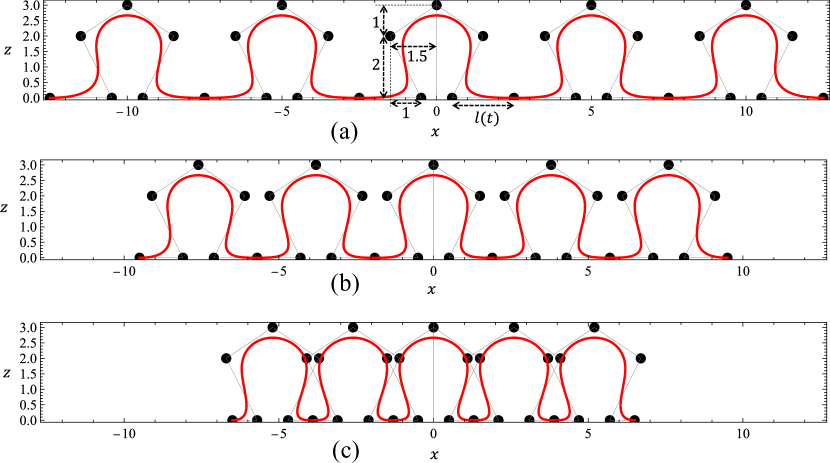
Figure 16: B-splines (red) of the control points (black) for three values of $t$: (a) $t=0$, (b) $t=10$, (c) $t=20$

Figure 16 shows how the control points of the B-spline function are constructed. A wrinkle is constructed from a set of five points whose relative distances are fixed. Midway between each pair of neighbouring pentagons there is an additional point at a time-dependent distance $l(t)=2.5-0.06t$. Thus, as time progresses, the pentagons rigidly translate towards $x=0$.

References

- [1] F Plum and D Labonte “scAnt-an open-source platform for the creation of 3D models of arthropods (and other small objects)” In PeerJ 9, 2021, pp. 1–29 DOI: 10.7717/peerj.11155
- [2] Stemmer Imaging “LMI Gocator 3000” URL: https://www.stemmer-imaging.com/en-gb/products/series/lmi-gocator-3100/
- [3] Canon Europe “3D photogrammetry explained” URL: https://www.canon-europe.com/pro/stories/3d-photogrammetry/
- [4] Harold Mytum and John Robert Peterson “The Application of Reflectance Transformation Imaging (RTI) in Historical Archaeology” In Historical Archaeology 52, 2018, pp. 489–503
- [5] M Limongello, S Antinozzi, L Vecchio and F Fiorillo “Digital survey and reconstruction for enhancing epigraphic readings with erode surface” In Journal of Physics: Conference Series 2204.1 IOP Publishing, 2022, pp. 012014 DOI: 10.1088/1742-6596/2204/1/012014
- [6] Rene Ranftl, Stefan Gehrig, Thomas Pock and Horst Bischof “Pushing the limits of stereo using variational stereo estimation” In IEEE Intelligent Vehicles Symposium, Proceedings, 2012, pp. 401–407 DOI: 10.1109/IVS.2012.6232171
- [7] S. Galliani, Katrin Lasinger and Konrad Schindler “Massively Parallel Multiview Stereopsis by Surface Normal Diffusion” In 2015 IEEE International Conference on Computer Vision (ICCV), 2015, pp. 873–881 URL: https://api.semanticscholar.org/CorpusID:9067666
- [8] L.M. Galantucci, M. Pesce and F. Lavecchia “A powerful scanning methodology for 3D measurements of small parts with complex surfaces and sub millimeter-sized features, based on close range photogrammetry” In Precision Engineering 43, 2016, pp. 211–219 DOI: https://doi.org/10.1016/j.precisioneng.2015.07.010
- [9] Lucio Tommaso De Paolis et al. “Photogrammetric 3D Reconstruction of Small Objects for a Real-Time Fruition” In Augmented Reality, Virtual Reality, and Computer Graphics Cham: Springer International Publishing, 2020, pp. 375–394
- [10] Antigoni Panagiotopoulou et al. “Super-Resolution Techniques in Photogrammetric 3D Reconstruction from Close-Range UAV Imagery” In Heritage 6.3, 2023, pp. 2701–2715 DOI: 10.3390/heritage6030143
- [11] Rasmus Jensen et al. “Large Scale Multi-view Stereopsis Evaluation” In 2014 IEEE Conference on Computer Vision and Pattern Recognition, 2014, pp. 406–413 DOI: 10.1109/CVPR.2014.59
- [12] Bryan D. Sandoval-Gaytan, Lili-Marlene Camacho and Carlos Vazquez-Hurtado “Point Cloud Generation of Transparent Objects: A Comparison between Technologies” In 2023 IEEE Global Engineering Education Conference (EDUCON), 2023, pp. 1–3 DOI: 10.1109/EDUCON54358.2023.10125143
- [13] Zhaoshuo Li et al. “Neuralangelo: High-Fidelity Neural Surface Reconstruction” In IEEE Conference on Computer Vision and Pattern Recognition (CVPR), 2023
- [14] Bojian Wu et al. “Full 3D Reconstruction of Transparent Objects” In ACM Trans. Graph. 37.4 New York, NY, USA: Association for Computing Machinery, 2018 DOI: 10.1145/3197517.3201286
- [15] Hillel Aharoni and Eran Sharon “Direct observation of the temporal and spatial dynamics during crumpling” In Nature materials 9, 2010, pp. 993–7 DOI: 10.1038/nmat2893
- [16] G.. Hinton and R.. Salakhutdinov “Reducing the Dimensionality of Data with Neural Networks” In Science 313.5786, 2006, pp. 504–507 DOI: 10.1126/science.1127647
- [17] Yann A. LeCun, Léon Bottou, Genevieve B. Orr and Klaus-Robert Müller “Efficient BackProp” In Neural Networks: Tricks of the Trade: Second Edition Berlin, Heidelberg: Springer Berlin Heidelberg, 2012, pp. 9–48 DOI: 10.1007/978-3-642-35289-8_3
- [18] Li Deng “The mnist database of handwritten digit images for machine learning research” In IEEE Signal Processing Magazine 29.6 IEEE, 2012, pp. 141–142
- [19] Kaiming He, Xiangyu Zhang, Shaoqing Ren and Jian Sun “Delving Deep into Rectifiers: Surpassing Human-Level Performance on ImageNet Classification” In 2015 IEEE International Conference on Computer Vision (ICCV), 2015, pp. 1026–1034 DOI: 10.1109/ICCV.2015.123
- [20] Shohei Kubota, Hideaki Hayashi, Tomohiro Hayase and Seiichi Uchida “Layer-Wise Interpretation of Deep Neural Networks using Identity Initialization” In ICASSP 2021 - 2021 IEEE International Conference on Acoustics, Speech and Signal Processing (ICASSP), 2021, pp. 3945–3949 DOI: 10.1109/ICASSP39728.2021.9414873
- [21] Diederik P. Kingma and Jimmy Ba “Adam: A Method for Stochastic Optimization” In CoRR abs/1412.6980, 2015
- [22] Herbert Edelsbrunner and Ernst P. Mücke “Three-Dimensional Alpha Shapes” In ACM Trans. Graph. 13.1 New York, NY, USA: Association for Computing Machinery, 1994, pp. 43–72 DOI: 10.1145/174462.156635
- [23] Zhongying Wang et al. “Wrinkled, wavelength-tunable graphene-based surface topographies for directing cell alignment and morphology” BIOMEDICAL APPLICATIONS OF CARBON NANOMATERIALS In Carbon 97, 2016, pp. 14–24 DOI: https://doi.org/10.1016/j.carbon.2015.03.040
- [24] I.. Bronshtein, K.. Semendyayev, Gerhard Musiol and Heiner Mühlig “Geometry” In Handbook of Mathematics Berlin, Heidelberg: Springer Berlin Heidelberg, 2015, pp. 129–268 DOI: 10.1007/978-3-662-46221-8_3