Non-intrusive model combination
for learning dynamical systems

Abstract

In data-driven modelling of complex dynamic processes, it is often desirable to combine different classes of models to enhance performance. Examples include coupled models of different fidelities, or hybrid models based on physical knowledge and data-driven strategies. A key limitation of the broad adoption of model combination in applications is intrusiveness: training combined models typically requires significant modifications to the learning algorithm implementations, which may often be already well-developed and optimized for individual model spaces. In this work, we propose an iterative, non-intrusive methodology to combine two model spaces to learn dynamics from data. We show that this can be understood, at least in the linear setting, as finding the optimal solution in the direct sum of the two hypothesis spaces, while leveraging only the projection operators in each individual space. Hence, the proposed algorithm can be viewed as iterative projections, for which we can obtain estimates on its convergence properties. To highlight the extensive applicability of our framework, we conduct numerical experiments in various problem settings, with particular emphasis on various hybrid models based on the Koopman operator approach.

1 Introduction

Model combination plays a crucial role in learning dynamics by bridging different approaches, effectively tackling difficulties like incomplete physical models [1, 2, 3, 4, 5], multi-fidelity data [6], and model stabilization [7]. The main idea behind model combination is to utilize domain knowledge to handle the difficulties caused by nonlinearity and high-dimensionality in complex dynamical systems. There are two primary ways where model combination can be beneficial. First, there may be partial physical models that can be leveraged, and data-driven components model the corrections to these models to improve prediction accuracy [8, 9, 10, 11, 12, 5]. Second, general structural information on the underlying dynamics may point to effective ways of model combination. For example, the Koopman operator approach [13, 14, 15] can effectively model nonlinear dynamics, but it requires the judicious choice of dictionary functions that becomes challenging for high-dimensional systems. However, for dynamics with a known structure such as reaction-diffusion equations, this difficulty can be alleviated by combining a high-dimensional linear model (diffusion) and a nonlinear point-wise Koopman model (reaction). The latter only requires the approximation of 1D functions, thus the choice of dictionary is much easier (see examples in section 4).

While model combination is desirable, the current algorithmic approaches suffer from two main limitations. The first is sub-optimality, which manifests itself in a number of works on “residual learning”, which learn data-driven corrections to existing theoretical models [2, 3, 4]. These methods first select a model in the known physical model space (the first hypothesis space) and then learn the correction using a data-driven method (the second hypothesis space). We will show in section 3 that in general, this approach does not give the best possible combined model, even if each of the above steps achieves minimal error individually in its fitting process. An alternative to the two steps process is to train the two models simultaneously. Examples include coupled physics-informed neural networks [1, 16], the combination of neural networks and the finite-element method [5] and the combination of linear and nonlinear neural networks for model stabilization [7]. Although these joint-training processes ensure better optimality, they bring about the second limitation of intrusiveness as implementing them typically requires significant modification to the underlying code. Non-intrusiveness is a highly desirable algorithmic property in the analysis of dynamical systems. For instance, in the context of model reduction, many studies employ neural networks to perform non-intrusive dimensionality reduction on commercial simulation software [17, 18]. Additionally, an intrusive approach to combination can give rise to additional challenges. For instance, certain data-driven methods have well-developed optimization techniques (e.g., we can achieve fast convergence when solving linear regression problems using the GMRES method [19]). Intrusively combining these two kinds of data-driven methods may result in the loss of the favorable properties associated with optimization. Also, the combination of two simple models could lead to a complex problem to be jointly solved. An example of this complexity is evident in robust principal component analysis [20], where the objective is to find a representation of the target matrix as a combination of one sparse matrix and one low-rank matrix. Taking into consideration the limitation above, proposing a non-intrusive model combination approach is a significant challenge in learning dynamics.

To tackle these challenges, in this work we propose an efficient framework, referred to as the iterative model combination algorithm, which provides a non-intrusive approach to combining two data-driven models through additive combination. Moreover, unlike residual learning, our approach is provably optimal in the linear setting when both hypothesis spaces are closed subspaces of a Hilbert space. In this case, the algorithm is equivalent to alternatively projecting the residual vector onto the orthogonal complements of the two hypothesis spaces respectively. We prove that our algorithm converges linearly, with explicit a priori and a posteriori estimates for the trajectory error. The latter can be used as a principled stopping criterion. Additionally, we introduce an accelerated version of this algorithm, which is highly efficient for specific classes of problems where one model hypothesis space is low-dimensional. We validate these methods across various problem settings, including diffusion-reaction equations, forced PDE-ODE coupled models in cardiac electrophysiology, and parameterized tail-accurate control systems, highlighting the extensive applicability of our framework. We pay particular attention to Koopman operator-based methods [13, 21, 22, 23] as candidate hypothesis spaces for data-driven methods, due to their wide applicability in learning nonlinear dynamics. Following this introduction, in section 2 we introduce the problem formulation of non-intrusive model combination in learning dynamical systems with a simple example of reaction-diffusion equation. In section 3, we propose a linearly convergent iterative model combination algorithm and its acceleration scheme. We then provide theoretical analysis and experimental evidence validating the convergence patterns. Section 4 showcases numerical results on three different problem settings and choices of model hypothesis spaces. Eventually, conclusions are prospects are drawn in section 5. The implementation of our method and the reproduction of presented experiments are found in [24].

2 Problem formulation

2.1 Learning dynamics by data-driven methods

Let us consider a dynamical system in state space $X\subset\mathbb{R}^{K}$ with a high-dimensional, nonlinear evolution function $F:X\to X$. The states $x_{k}\in X$ satisfy $x_{k+1}=F(x_{k})$ for $k=0,1,2,3,\ldots,N$. Our objective is to learn the evolution function $F$ using data-driven methods and then address both predictive and control problems for this dynamical system. That is, we aim to find a model $\tilde{F}$ such that

$$\tilde{F}=\mathrm{argmin}_{\hat{F}\in\mathcal{G}}\mathbb{E}[L(F(x),\hat{F}(x))].$$ (1)

In this context, $\mathcal{G}$ is the hypothesis space of a selected data-driven model class, $\mathbb{E}$ represents the expectation over the distribution of states $x$, and $L(y,\hat{y})$ is the loss function which measures how different the prediction of a hypothesis $\hat{F}$ is from that of the true outcome $F$. Here, we choose the loss function $L(y,\hat{y})$ as mean square error

$$L(y,\hat{y})=\|y-\hat{y}\|^{2}.$$ (2)

For illustration, in this paper we abstract the fitting or learning process on data generated by a ground truth dynamics driven by $F$ (i.e, solving the minimization problem (1)), using a hypothesis space $\mathcal{G}$ as a projection operator $P_{\mathcal{G}}$

$$\tilde{F}=P_{\mathcal{G}}(F)=\mathrm{argmin}_{\hat{F}\in\mathcal{G}}\|F-\hat{F}\|.$$ (3)

which means the optimal solution of minimization problem (1) is a projection of $F$ onto the hypothesis space $\mathcal{G}$.

Suppose we have some snapshots ${x_{0}^{j},x_{1}^{j},\ldots,x_{k}^{j},\ldots,x_{m}^{j}}$ from a set of trajectories generated from initial values $x_{0}^{j},\ j=1,2,3,\ldots,s$. We can rearrange these snapshots into a set of pairs $\mathcal{D}=[(x_{k}^{j},x_{k+1}^{j})],\ k=0,1,2,\ldots,m-1,\ j=1,2,3,\ldots,s$. Since calculating the expectation over the entire state set $X$ is challenging, we typically solve the optimization problem based on empirical risk:

$$\tilde{F}=\mathrm{argmin}_{\hat{F}\in G}\sum_{(x,y)\in\mathcal{D}}L(y,\hat{F}(x)).$$ (4)

For convenience, in presenting our method and analysis, we do not distinguish between the solutions of the optimization problems in (1) and (4).

Numerous machine learning techniques can be employed as the described projection. For example, linear regression involves projecting onto a linear subspace defined by explanatory variables. The Koopman operator approximates the evolution function projected onto a linear subspace spanned by the dictionary observables [15]. Similarly in the nonlinear case, neural networks [25] act as solvers for projecting onto a nonlinear composition function space.

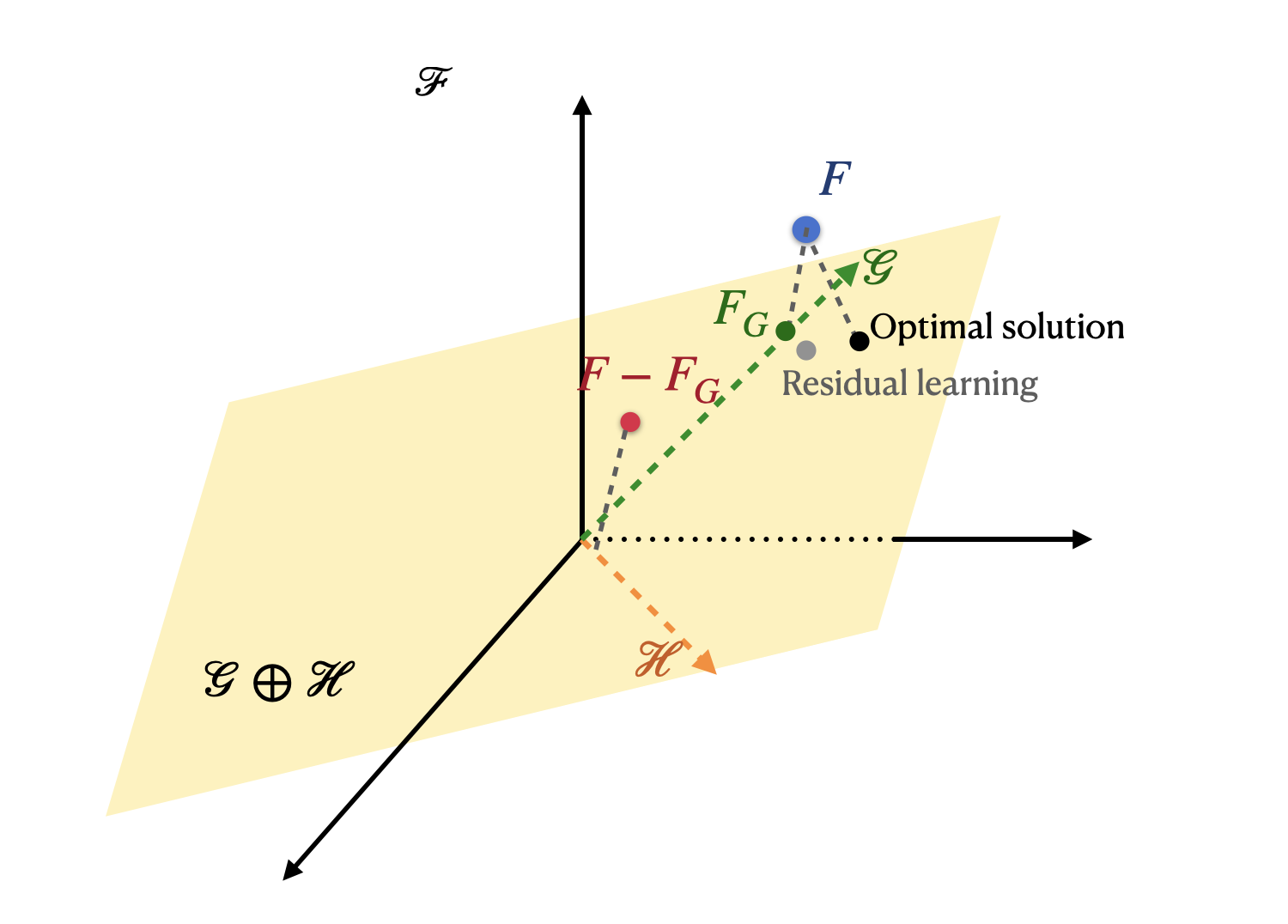
Figure 1: A cartoon for model combination. Suppose we aim to understand the evolution function $F$ within a broad, high-dimensional space denoted as $\mathcal{F}$. We can break down the model into two lower-dimensional components, $\mathcal{G}$ and $\mathcal{H}$, and subsequently learn $F$ within a direct-sum subspace. $P_{\mathcal{G}\oplus\mathcal{H}}(F)$ is plotted as the black point in the yellow plane, which represents the optimal approximation. However, if we conduct the residual learning process, projecting $F$ to $\mathcal{G}$ to find $F_{\mathcal{G}}$ (the green point) and then project the residual $F-F_{\mathcal{G}}$ (the red point) onto $\mathcal{H}$, the final solution is plotted as the grey point, which is visually not the optimal approximation.

2.2 An example: reaction-diffusion equation

Purely data-driven methods may face challenges in learning dynamics due to high dimensionality and complexity of dynamical systems. However, combining models can effectively solve this problem. High-dimensional problems can often be decomposed into a number of much simpler problems using a divide and conquer strategy and modelling different parts of dynamics with different data-driven methods. Additionally, if some structural information about the dynamics is already known, combining models can help incorporate this prior knowledge to enhance prediction or control performance.

Here, we illustrate the benefits of model combination with a simple example of reaction-diffusion equation:

$$\frac{du}{dt}=\mu\frac{d^{2}u}{dz^{2}}+R_{\eta}(u).$$ (5)

In this equation, $u(z,t)$ is a one-dimensional variable, $z\in[0,1]$ and $t\in[0,0.05]$. $u(z,0)$ is randomly selected following uniform distribution in $[0,1]$ after discretization, and $u(0,t)=u(1,t)=0$. We observe that (5) can be divided into two distinct components: the diffusion term $u(z,t)\mapsto\mu\frac{d^{2}u}{dz^{2}}(z,t)$ represents a linear model which is related to the space complexity of the discretization, while the reaction term $u(z,t)\mapsto R_{\eta}(u(z,t))$ is a nonlinear and pointwise function that depends on a parameter $\eta$, but remains independent of the spatial dimension. Considering this information, we can model these two components separately and add them together. One involves learning the diffusion term as a linear model that relates $u(z_{i},t_{j+1})$ to $u(z_{i},t_{j})$ and its neighboring values. The other part involves learning the reaction term as a nonlinear problem based on $u(z_{i},t_{j})$ for any $z_{i}$ within the discretization mesh. This combination can decompose the high-dimensional problem into simpler components while preserving the structure of the reaction-diffusion equation. An example of application of this scheme is the data-driven modelling of intrinsic self-healing materials [26]. Detailed numerical results for learning the reaction-diffusion equation are presented in section 4.2. Furthermore, if we consider a control problem involving the adjustment of $\mu$ in (5), we can model the equation as two parts: $u_{n+1}=F_{1}(u_{n},\mu)+F_{2}(u_{n},\eta)$, and maintain the convexity of the optimization problem through specific structures for $F_{1}$ and $F_{2}$. A numerical example of this type is shown in section 4.4.

2.3 General problem formulation of model combination

With the previous motivation in mind, let us now introduce the general formulation of model combination. We start with the direct-sum space: for two subsets $\mathcal{G}$ and $\mathcal{H}$ of a Hilbert space, the direct-sum space of $\mathcal{G}$ and $\mathcal{H}$ is defined as:

$$\mathcal{G}\oplus\mathcal{H}=\{F_{\mathcal{G}}+F_{\mathcal{H}}:F_{\mathcal{G}}\in\mathcal{G},F_{\mathcal{H}}\in\mathcal{H}\}.$$ (6)

Suppose we have two methods that can respectively obtain the projection in the hypothesis spaces $\mathcal{G}$ and $\mathcal{H}$, and the snapshots of the dynamical system $(X,F,x_{0})$ are known. In the combination of two models, we aim to approximate the evolution function $F$ in the direct-sum space of $\mathcal{G}$ and $\mathcal{H}$, i.e.,

$$\begin{split}\tilde{F}&=\mathrm{argmin}_{\hat{F}\in\mathcal{G}\oplus\mathcal{H}}\|F-\hat{F}\|\\ &=\tilde{F}_{\mathcal{G}}+\tilde{F}_{\mathcal{H}},\\ \mathrm{where}\quad\tilde{F}_{\mathcal{G}},\tilde{F}_{\mathcal{H}}&=\mathrm{argmin}_{\hat{F}_{\mathcal{G}}\in\mathcal{G},\hat{F}_{\mathcal{H}}\in\mathcal{H}}\|F-(\hat{F}_{\mathcal{G}}+\hat{F}_{\mathcal{H}})\|.\\ \end{split}$$ (7)

The notation of projection is described in (3) and the hypothesis spaces $\mathcal{G},\mathcal{H}$ are subsets in a Hilbert space.

According to the discussion of non-intrusiveness in section 1, we assume that we only have access to the projection operators for each individual hypothesis space. This can be legacy codes or highly optimized available routines. A key challenge in addressing the optimization problem is to find the optimal solution $\tilde{F}_{\mathcal{G}}+\tilde{F}_{\mathcal{H}}$ in a non-intrusive manner. In other words, we only have access to $P_{\mathcal{G}}$ and $P_{\mathcal{H}}$, and do not have access to the projection operator onto $\mathcal{G}\oplus\mathcal{H}$, corresponding to the learning algorithms already developed for each hypothesis space. The formulation of non-intrusive model combination is thus: how can we obtain an approximation $\tilde{F}$ in (7) using only the individual learning algorithms $P_{\mathcal{G}}$ and $P_{\mathcal{H}}$? In section 3, we propose an algorithm to address this problem.

3 Methodology

3.1 Non-optimality of the residual learning

Since solving for the optimal solution jointly might not be possible in a non-intrusive manner, the goal is to identify the corresponding $F_{\mathcal{G}}\in\mathcal{G}$ and $F_{\mathcal{H}}\in\mathcal{H}$ through the individual models. One approach to address this problem, referred to as residual learning [2, 3], involves obtaining an initial $F_{\mathcal{G}}$ within the hypothesis space $\mathcal{G}$ and subsequently, employing a correction model $P_{\mathcal{H}}$ to learn and refine the difference $F-F_{\mathcal{G}}$. This leads to an integrated approximation denoted as $F\approx F_{\mathcal{G}}+P_{\mathcal{H}}(F-F_{\mathcal{G}})$. However, the selection of an appropriate $F_{\mathcal{G}}$ could be a challenging task. One potential strategy is to utilize a fitting process to choose the approximation $F_{\mathcal{G}}=P_{\mathcal{G}}(F)$ of $F$ within $\mathcal{G}$.

Nonetheless, this residual learning process may not yield the closest approximation, even in simple problem settings. We visually illustrate the failure of residual learning using figure 1. Here, we first project $F$ (the blue point) onto the subspace $\mathcal{G}$, and then learn a correction by projecting $F-F_{\mathcal{G}}$ (the red point) onto the subspace $\mathcal{H}$. We can immediately observe that the residual learning procedure does not give the best approximation in the direct sum space. We will show later in section 4.2 that for typical problems, residual learning is non-optimal.

3.2 The iterative model combination algorithm

By observing figure 1, a logical progression of residual learning would be to cyclically perform the correction process. Starting from an initial guess $F_{\mathcal{H}}^{0}$ (often taken to be 0), we iteratively perform the following learning steps

$$\begin{split}F_{\mathcal{G}}^{n}\leftarrow P_{\mathcal{G}}(F-F_{\mathcal{H}}^{n}),\\ F_{\mathcal{H}}^{n+1}\leftarrow P_{\mathcal{H}}(F-F_{\mathcal{G}}^{n}),\end{split}$$ (8)

until some stopping criterion is met. It is worth noting that residual learning only conducts this iterative step once, which is not theoretically optimal. In contrast, we provide in section 3.3 a theoretical analysis of our method in the special case where $\mathcal{G},\mathcal{H}$ are closed subspaces. In particular, we show that the method exhibits a linear convergence pattern. Furthermore, the convergence rate is related to the correlation between the two hypothesis spaces, a notion that can be made precise in the linear setting.

We summarize the proposed method in Algorithm 1. The stopping criterion used in our numerical experiments is

$$\frac{1}{N}\sum_{i=0}^{N}\|y^{n}_{i}-y_{i}\|<\epsilon.$$ (9)

Here, $y_{i}^{n}$ represents the one-step prediction generated from the initial condition $x_{i}$ by $F^{n}=F^{n}_{\mathcal{G}}+F^{n}_{\mathcal{H}}$, and $y_{i}$ comes from the real trajectory data, where $y_{i}=F(x_{i})$. Other stopping criteria can also be used, as described in the a priori and posteriori estimates provided in section 3.3, such as

$$\frac{1}{N}\sum_{i=0}^{N}\|y^{n}_{i}-y^{n-1}_{i}\|<\epsilon.$$ (10)

Algorithm 1 The iterative model combination algorithm

Data-driven models functioning as projection operators $P_{\mathcal{G}}$ and $P_{\mathcal{H}}$

$n\leftarrow 0$

$F_{\mathcal{H}}^{n}\leftarrow P_{\mathcal{H}}(F)$ $\triangleright$ Get the best approximation of $F$ by $P_{\mathcal{H}}$

while stopping criterion is not satisfied do

     $F_{\mathcal{G}}^{n}\leftarrow P_{\mathcal{G}}(F-F_{\mathcal{H}}^{n})$ $\triangleright$ Get the best approximation of $F-F_{\mathcal{H}}$ by $P_{\mathcal{G}}$

     $F_{\mathcal{H}}^{n+1}\leftarrow P_{\mathcal{H}}(F-F_{\mathcal{G}}^{n})$ $\triangleright$ Get the best approximation of $F-F_{\mathcal{G}}$ by $P_{\mathcal{H}}$

     $n\leftarrow n+1$

end while

$\tilde{F}=F_{\mathcal{H}}^{n}+F_{\mathcal{G}}^{n}$ $\triangleright$ Obtain the best approximation in $\mathcal{H}\oplus\mathcal{G}$

3.3 Convergence analysis

In this part, we give a theoretical analysis on convergence of iterative model combination algorithm (Algorithm 1) in the subspace case. The key idea in our analysis is the observation that our algorithm is essentially an iterative projection of the residual $F-F_{\mathcal{H}}^{0}$ onto the orthogonal complements $\mathcal{G}^{\perp}$ of $\mathcal{G}$ and $\mathcal{H}^{\perp}$ of $\mathcal{H}$ respectively. Hence, the convergence and its rate follow from the alternative projection method proposed by John von Neumann [27] to find the intersection of two closed subspaces. This projection algorithm was later extended to convex sets by Dykstra [28] and applied to multivariate regression problems [29] and robust principal component analysis [20].

After presenting the convergence of the approximations ${F}^{n}:=F^{n}_{\mathcal{G}}+F^{n}_{\mathcal{H}}$, we provide estimates for the $k$-step predictive error after $n$ iterations, denoted as $e_{k}^{n}=\|x_{k}^{n}-x_{k}\|$. Estimates of the limiting value of this error, denoted as $e_{k}=\lim_{n\to+\infty}e_{k}^{n}$, are also presented. Here, $x_{k}^{n}$ represents the predicted state at time $k$ based on the $n$-th iteration, while ${x_{k}}$ represents the actual trajectory data. For all the theorems discussed in this section, we assume that the dynamical system and models have the following properties in assumption 1.

Assumption 1.

1. $\mathcal{H}$ and $\mathcal{G}$ are closed linear subspaces of a Hilbert space.

2. $F^{n}_{\mathcal{G}}$ and $F^{n}_{\mathcal{H}}$ are iteratively computed by Algorithm 1.

3. The set of states $X\subset\mathbb{R}^{K}$ is bounded, and we denote $M=\max_{x\in X}\|x\|$.

4. For illustrative purposes, we assume $\|F\|=1$.

We will now provide an analysis of the convergence of Algorithm 1.

Theorem 1 (Convergence).

Under assumption 1, the following holds:

1. $\lim_{n\to+\infty}\|P_{\mathcal{G}\oplus\mathcal{H}}(F)-F^{n}\|=0$.

2. As $n\to\infty$, the predicted trajectory $\{x^{n}_{k}\}$ converges to some $\{\tilde{x}_{k}\}$. Suppose the distance between $F$ and $\mathcal{G}\oplus\mathcal{H}$ equals to $\epsilon_{F}$. For any finite $k\in\mathbb{Z}^{+}$, the following inequality holds:

   $$e_{k}=\|\tilde{x}_{k}-x_{k}\|\leq((1+\epsilon_{F})^{k}-1)M.$$ (11)

   In particular, when $\epsilon_{F}=0$,

   $$\lim_{n\to+\infty}e^{n}_{k}=0,\quad\forall k\in\mathbb{Z}^{+}.$$ (12)

Theorem 1 demonstrates that as $n\to+\infty$, the evolution function obtained through Algorithm 1 converges to the projection of $F$ onto the direct-sum space $\mathcal{G}\oplus\mathcal{H}$. Additionally, the predicted trajectory also converges. The distance between the converged prediction and the reference trajectory can be controlled, and the distance is 0 when $F$ is in $\mathcal{G}\oplus\mathcal{H}$. The detailed proof is shown in A.1.

To further analyze the estimate of the convergence rate, we introduce the definition of minimum angle between subspaces [30]. This concept provides a mathematical measure that will help understand the relationship between the convergence rate and the chosen models spaces.

Definition 1 (Minimum angle between subspaces).

We define $\theta_{0}(\mathcal{G},\mathcal{H})$ as the minimum angle between subspaces. $c_{0}(\mathcal{G},\mathcal{H})=\cos(\theta_{0}(\mathcal{G},\mathcal{H}))$ is given by

$$\sup\{|\langle g,h\rangle|:g\in\mathcal{G},\|g\|\leq 1,h\in\mathcal{H},\|h\|\leq 1\}.$$ (13)

Define $c(\mathcal{G},\mathcal{H})=c_{0}(\mathcal{G}\cap(\mathcal{G}\cap\mathcal{H})^{\bot},\mathcal{H}\cap(\mathcal{G}\cap\mathcal{H})^{\bot})$, then $0\leq c(\mathcal{G},\mathcal{H})\leq c_{0}(\mathcal{G},\mathcal{H})\leq 1$, where $\mathcal{G}^{\bot}$, $\mathcal{H}^{\bot}$ represent the orthogonal complements of $\mathcal{G}$, $\mathcal{H}$.

Theorem 2 (Convergence rate).

Under assumption 1, the following conclusions hold:

1. For all $n\in\mathbb{Z}^{+}$, $\|F^{n}-P_{\mathcal{G}\oplus\mathcal{H}}(F)\|\leq c(\mathcal{G},\mathcal{H})^{2n-1}$.

2. For any finite $k\in\mathbb{Z}^{+},n\in\mathbb{Z}^{+}$, the following inequality holds:

   $$e_{k}^{n}=\|x^{n}_{k}-x_{k}\|\leq[(1+c(\mathcal{G},\mathcal{H})^{2n-1}+\epsilon_{F})^{k}-1]M.\\$$ (14)

3. Specifically, if $F\in\mathcal{G}\oplus\mathcal{H}$, then

   $$e_{k}^{n}=\|x^{n}_{k}-x_{k}\|\leq[(1+\|F-F^{n}\|)^{k}-1]M$$ (15)

   $$e_{k}^{n}=\|x^{n}_{k}-x_{k}\|\leq[(1+\frac{c^{2}(\mathcal{G},\mathcal{H})}{1-c^{2}(\mathcal{G},\mathcal{H})}\|F^{n}-F^{n-1}\|)^{k}-1]M$$ (16)

   Furthermore, when $k\|F-F^{n}\|\leq 1,\ k\frac{c^{2}(\mathcal{G},\mathcal{H})}{1-c^{2}(\mathcal{G},\mathcal{H})}\|F^{n}-F^{n-1}\|<1$, we have

   $$e_{k}^{n}\leq k^{2}M\|F-F^{n}\|.$$ (17)

   $$e_{k}^{n}\leq k^{2}M\frac{c(\mathcal{G},\mathcal{H})}{1-c^{2}(\mathcal{G},\mathcal{H})}\|F^{n}-F^{n-1}\|.$$ (18)

These inequalities indicate that the error between $F^{n}$ and $P_{\mathcal{G}\oplus\mathcal{H}}(F)$ decreases exponentially with the number of iterations, with a rate determined by the value of $c(\mathcal{G},\mathcal{H})$. Also, when $F\in\mathcal{G}\oplus\mathcal{H}$, the a posteriori estimate of Algorithm 1 presents clear evidence that the prediction error $e_{k}^{n}$ is predominantly governed by the absolute difference between two successive estimated functions, namely $\|F^{n}-F^{n-1}\|$. The proof of theorem 2 is shown in A.2. According to the estimates, we could establish a suitable stopping criterion as (9) and (10).

Additionally, theorem 2 could serve as a criterion for method design. One may observe that $c(\mathcal{G},\mathcal{H})$ measures the ‘orthogonality’ between $\mathcal{G}$ and $\mathcal{H}$. In other words, if the two models describe independent features of the problem, the algorithm will converge rapidly. Otherwise, when the correlation between the two models increases, the convergence speed may be slower. Thus, if one hypothesis space $\mathcal{G}$ is chosen, we can solve an optimization problem over the parameterized set of hypothesis spaces $\mathcal{H}_{\nu}$ with the hyper-parameter $\mu$

$$\min_{\nu}c(\mathcal{G},\mathcal{H_{\nu}})$$ (19)

to find a particular hypothesis space $\mathcal{H}_{\nu^{*}}$ which maximizes performance.

We now validate these theoretical conclusions with a simple numerical example.

Numerical verification.

In order to evaluate the convergence pattern in theoretical analysis, we consider a linear PDE in the form of a diffusion equation

$$\frac{du}{dt}=\mu_{1}\frac{d^{2}u}{dz_{1}^{2}}+\mu_{2}\frac{d^{2}u}{dz_{2}^{2}}.$$ (20)

In this equation, $u(z,t)$ is a one-dimensional variable where $z\in\Omega=[0,1]^{2}$ and $t\in[0,0.05]$. After discretization, $u(z,0)$ is randomly selected from a uniform distribution $U(0,1)$ independently for each $z$, and the boundary condition is $u(z,t)$ for all $z$ in the boundary $\partial\Omega$ equals to 0 (i.e., homogeneous Dirichlet boundary conditions).

We choose two parametric hypothesis spaces as follows:

$$\begin{split}\mathcal{G}:F_{\mathcal{G}}(u_{ij}^{n};\lambda_{1})=\lambda_{1}\delta^{2}_{z_{1}}u^{n}_{ij},\\ \mathcal{H}:F_{\mathcal{H}}(u_{ij}^{n};\lambda_{2})=\lambda_{2}(\nu\delta^{2}_{z_{1}}u^{n}_{ij}+\delta^{2}_{z_{2}}u^{n}_{ij}),\\ \end{split}$$ (21)

where $\lambda_{1},\lambda_{2}$ are the trainable parameters. Here, $\delta_{z_{1}}^{2}u,\delta_{z_{2}}^{2}u$ represent the discretization of $\frac{d^{2}u}{dz_{1}^{2}},\frac{d^{2}u}{dz_{2}^{2}}$, as

$$\begin{split}\delta_{z_{1}}^{2}u^{n}_{ij}=\frac{u^{n}_{i-1,j}-2u^{n}_{ij}+u^{n}_{i+1,j}}{(\Delta{z_{1}})^{2}},\\ \delta_{z_{2}}^{2}u^{n}_{ij}=\frac{u^{n}_{i,j-1}-2u^{n}_{ij}+u^{n}_{i,j+1}}{(\Delta{z_{2}})^{2}}.\\ \end{split}$$ (22)

$\Delta z_{1}$ and $\Delta z_{2}$ are chosen as $0.1$ in our experiments.

The hyper-parameter $\nu$ in the hypothesis space $\mathcal{H}$ can influence the correlation between the two models. As $\nu$ increases from $0$, the correlation between the two models also increases. By theorem 2, we can obtain the inequality

$$\log(\|F^{n}-P_{\mathcal{G}\oplus\mathcal{H}}(F)\|)\leq(2n-1)c(\mathcal{G},\mathcal{H})+\log(\|F\|).$$ (23)

To validate our theoretical analysis, we conduct experiments with different values of $\nu$ (ranging from 0 to 2). From figure 2(a), we observe that as the correlation between the two models increases (i.e., larger values of $\nu$), the convergence speed becomes significantly slower. This indicates the crucial impact of ‘orthogonality’ on the convergence behavior of our iterative model combination algorithm. Additionally, we used the BFGS method to solve the optimization problem (19) and obtained the optimal value of $\nu$, represented as $\tilde{\nu}=-0.6455$. As depicted in figure 2(a), Algorithm 1 converges directly to the optimal solution, highlighting the effectiveness of adaptive model selection.

Figure 2(b) illustrates the convergence rate of Algorithm 1 across varying values of the orthogonality parameter $\nu$, with $n$ denoting the iteration steps. The two models could be written as inner products of vectors:

$$\begin{split}F_{\mathcal{G}}(u_{ij}^{n};\lambda_{1})=\lambda_{1}\mathbf{b_{1}}^{T}\mathbf{u}\\ F_{\mathcal{H}}(u_{ij}^{n};\lambda_{2})=\lambda_{2}(\nu\mathbf{b_{1}}+\mathbf{b_{2}})^{T}\mathbf{u}\end{split}$$ (24)

Here, $\mathbf{b_{1}}=[1,1,-2,0,0]^{T},\leavevmode\nobreak\ \mathbf{b_{2}}=[0,0,-2,1,1]^{T}$ and $\mathbf{u}=[u_{i-1,j}^{n},u_{i+1,j}^{n},u_{i,j}^{n},u_{i,j-1}^{n},u_{i,j+1}^{n}]^{T}$. We can calculate $c(\mathcal{G},\mathcal{H})$ by (25):

$$c(\mathcal{G},\mathcal{H})=\frac{\langle\mathbf{b_{1}},\nu\mathbf{b_{1}}+\mathbf{b_{2}}\rangle}{\|\mathbf{b_{1}}\|\|\nu\mathbf{b_{1}}+\mathbf{b_{2}}\|}=\sqrt{1-\frac{5}{9\nu^{2}+12\nu+9}}.$$ (25)

We could easily determine that the optimal value of $\nu$ is approximately $-0.667$ in (25). This value closely aligns with the optimal value obtained through numerical methods, $\tilde{\nu}$.

In figure 2(b), we evaluate both the reference and experimental convergence rates for varying $\nu$. The reference rate is computed using (25), while the experimental rates are determined as the slopes of $\log(\|F^{n}-P_{\mathcal{G}\oplus\mathcal{H}}(F)\|)$ relative to $2n-1$. Comparing our experimental rates with the reference values, we observe a close match. These results quantitatively support our theoretical analysis.

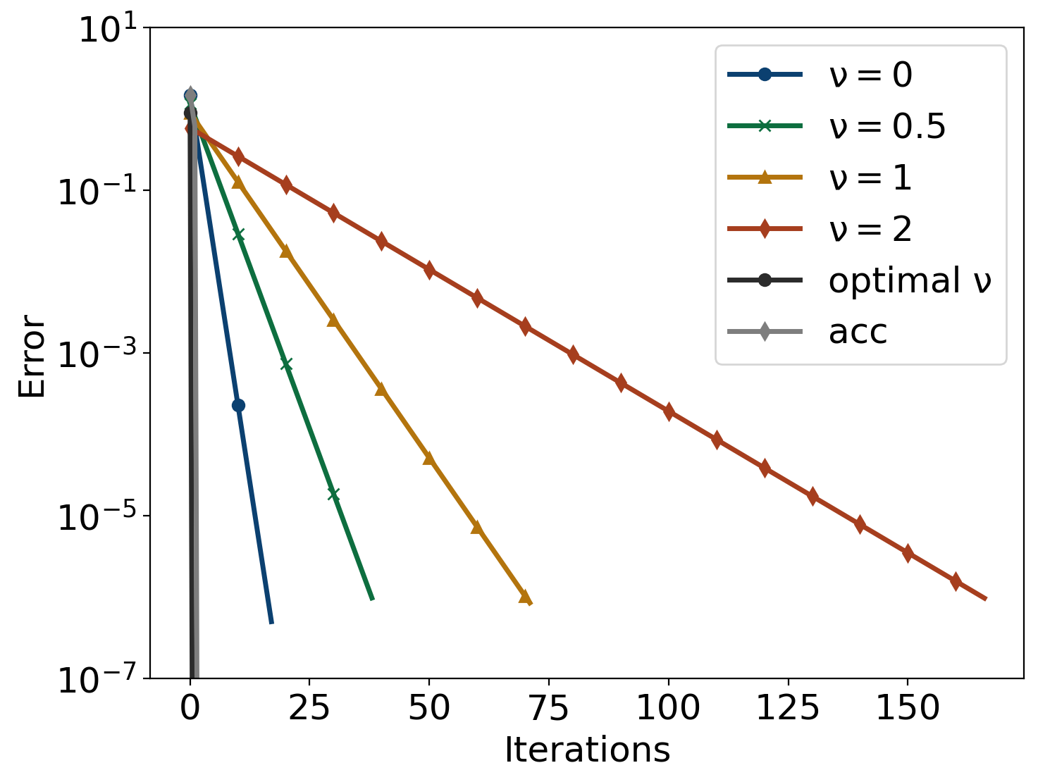
(a) The difference $\|F^{n}-P_{\mathcal{G}\oplus\mathcal{H}}(F)\|$ after $n$ iterations

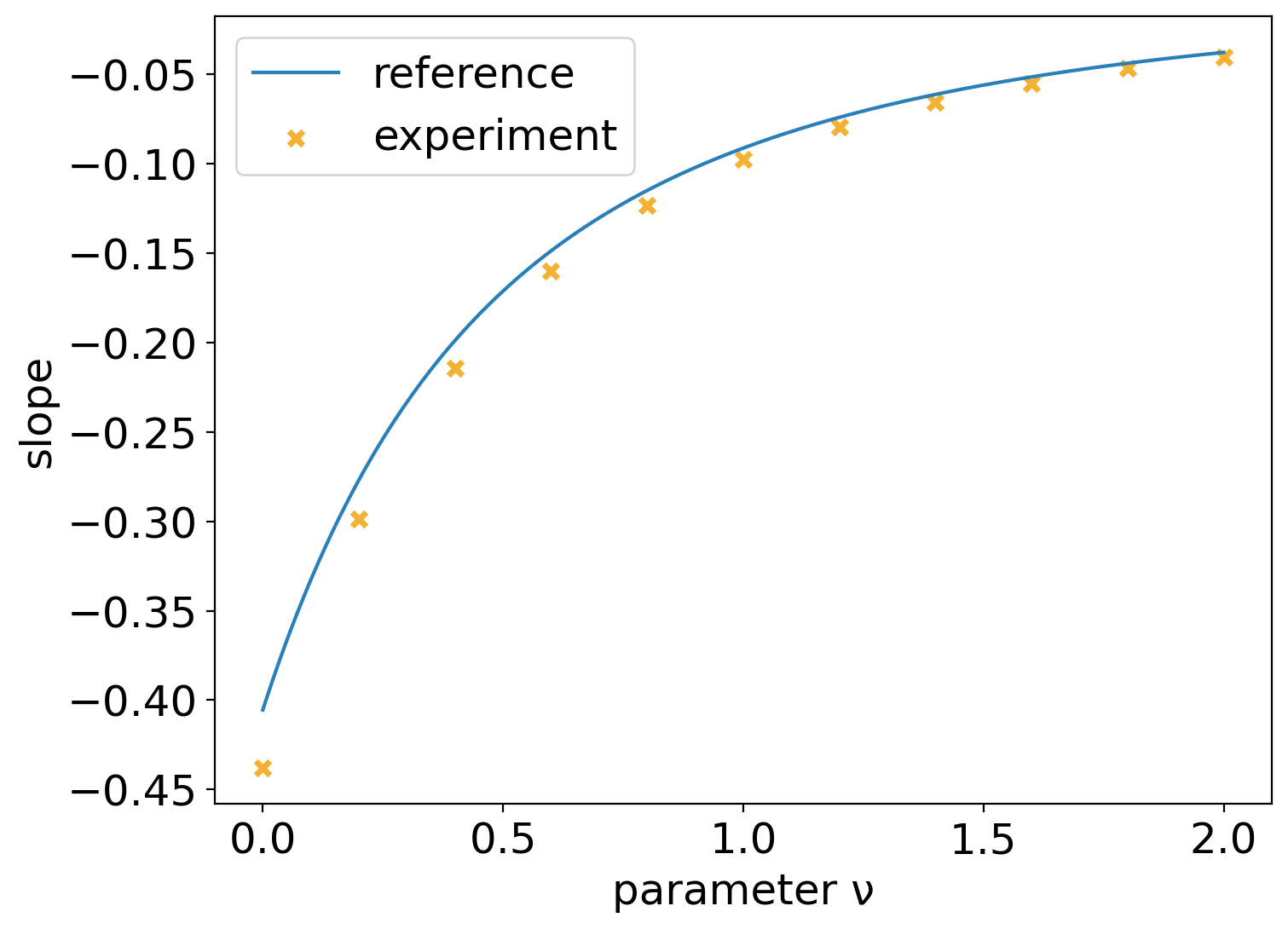
(b) The convergence rate: slope of $\log(\|F^{n}-P_{\mathcal{G}\oplus\mathcal{H}}(F)\|)$

Figure 2: Convergence rates for different hyper-parameter values ($\nu$): Left - Iteration differences by original scheme (Algorithm 1) for $\nu=0,0.5,1,2$ and optimal values, and that by acceleration scheme (Algorithm 2); Right - Reference and experimental convergence rates.

3.4 Acceleration scheme

In section 3.3, we have demonstrated that our algorithm is equivalent to an alternative approach involving the projection of the residual $r^{n}=F-F^{n}$ onto the complementary spaces $\mathcal{G}^{\bot}$ and $\mathcal{H}^{\bot}$ of $\mathcal{G}$ and $\mathcal{H}$, with a proof in A.1. Consequently, the residual $r^{n}$ converges to the projection of $F$ onto the intersection of the complementary spaces $\mathcal{G}^{\bot}\cap\mathcal{H}^{\bot}$. In a specific case where $F\in\mathcal{G}\oplus\mathcal{H}$, it yields $P_{\mathcal{G}^{\bot}\cap\mathcal{H}^{\bot}}(F)=0$. To accelerate the convergence of $r^{n}$ towards zero, we introduce an adaptive parameter $t_{F}$ in front of $(r^{n}-r^{n-1})$, rather than employing a straightforward update like $r^{n}=r^{n-1}+(r^{n}-r^{n-1})$. In other words, we solve the minimization problem

$$t_{F}=\mathrm{argmin}_{\hat{t}_{F}}(\langle r^{n-1}+\hat{t}_{F}(r^{n}-r^{n-1}),r^{n-1}+\hat{t}_{F}(r^{n}-r^{n-1})\rangle).$$ (26)

The optimal parameter $t_{F}$ is determined as:

$$t_{F}=\frac{\langle r^{n-1},r^{n-1}-r^{n}\rangle}{\langle r^{n-1}-r^{n},r^{n-1}-r^{n}\rangle}.$$ (27)

The acceleration algorithm, outlined in Algorithm 2, is based on the scheme proposed and analyzed in [31], and we show here that it has superior performance when at least one of the hypothesis spaces is low-dimensional. In fact, if either $\mathcal{G}$ or $\mathcal{H}$ has only one degree of freedom, we could claim that $r^{n}$ and $r^{n-1}$ are guaranteed to be linearly dependent (see a detailed proof in A.3). Hence, convergence is achieved with only a single step of acceleration. Experimental results in figure 2(a) validate this finding: regardless of the parameter $\nu$, Algorithm 2 converges after just one step. Furthermore, the experiment in section 4.2 shows similar results.

Algorithm 2 Acceleration scheme of iterative model combination algorithm

Data-driven models functioning as projection operators $P_{\mathcal{G}}$ and $P_{\mathcal{H}}$

$n\leftarrow 0$

$F_{\mathcal{H}}^{n}\leftarrow P_{\mathcal{H}}(F)$ $\triangleright$ Get the best approximation of $F$ by $P_{\mathcal{H}}$

$F_{\mathcal{G}}^{n}\leftarrow P_{\mathcal{G}}(F-F_{\mathcal{H}}^{n})$ $\triangleright$ Get the best approximation of $F-F_{\mathcal{H}}$ by $P_{\mathcal{G}}$

$F^{n}\leftarrow F^{n}_{\mathcal{H}}+F^{n}_{\mathcal{G}}$

while stopping criterion is not satisfied do

     $n\leftarrow n+1$

     $F_{\mathcal{H}}^{n}\leftarrow P_{\mathcal{H}}(F-F_{\mathcal{G}}^{n-1})$ $\triangleright$ Get the best approximation of $F-F_{\mathcal{G}}$ by $P_{\mathcal{H}}$

     $F_{\mathcal{G}}^{n}\leftarrow P_{\mathcal{G}}(F-F_{\mathcal{H}}^{n})$ $\triangleright$ Get the best approximation of $F-F_{\mathcal{H}}$ by $P_{\mathcal{G}}$

     $F^{n}\leftarrow F_{\mathcal{H}}^{n}+F_{\mathcal{G}}^{n}$

     $t_{F}\leftarrow\langle F-F^{n-1},F^{n-1}-F^{n}\rangle/\|F^{n-1}-F^{n}\|^{2}$ $\triangleright$ Calculate the parameter

     $F_{\mathcal{G}}^{n}\leftarrow t_{F}F_{\mathcal{G}}^{n}+(1-t_{F})F_{\mathcal{G}}^{n-1}$ $\triangleright$ Acceleration

end while

$\tilde{F}=F_{\mathcal{H}}^{n}+F_{\mathcal{G}}^{n}$ $\triangleright$ Obtain the best approximation in $\mathcal{H}\oplus\mathcal{G}$

4 Numerical experiments

We conduct experiments in three different problem settings, involving both predictive and control problems within parameterized dynamical systems. In the numerical results, we primarily construct linear models using linear regression and employ Koopman-type models to handle the nonlinear aspects. We have chosen Koopman models as an example in our numerical results due to the well-established data-driven methods available for Koopman models and the nature of the Koopman operator, which enables the transformation of nonlinear dynamical systems into a linear, infinite-dimensional representation that can be further truncated.

4.1 Basics on Koopman models

We now give a brief introduction of Koopman operator-based methods to learn dynamical systems. The reader is referred to [13] for a more comprehensive review. Consider a nonlinear dynamical system $x_{n+1}=F(x_{n})$ where $x_{i}\in X\subset\mathbb{R}^{k}$ and $F:X\to X$ is a nonlinear function. Instead of the dynamics on state spaces, the Koopman operator approach considers the dynamics on the space of observables, consisting of functions $\psi:X\to\mathbb{R}$ (or $\mathbb{C}$). We observe that if we consider the set of all such observables, its time evolution is $\psi(x_{n})\mapsto\psi({x_{n+1}})=\psi(F(x_{n}))\equiv\mathcal{K}\psi(x_{n})$, where $\mathcal{K}$ is the Koopman operator, a linear operator defined by

$$\mathcal{K}\psi=\psi\circ F.$$ (28)

To obtain a finite-dimensional representation of the Koopman operator, we construct a finite subspace spanned by a set of dictionary functions $\Psi=\{\psi_{1},\psi_{2},\psi_{3},\ldots,\psi_{N}\}$. Assuming this is an approximately $\mathcal{K}$-invariant subspace, we obtain a finite-dimensional approximation of the Koopman operator

$$\Psi(x_{n+1})=K\Psi(x_{n}).$$ (29)

Data-driven Koopman models have attracted significant attention in recent years, and several mature models for learning nonlinear dynamics have been proposed, such as Extended Dynamic Mode Decomposition (EDMD) [15] and machine-learning aided extensions [21, 32, 33]. Moreover, extended structures for parameterized Koopman models [15, 22] and structures for control problems [22, 23] have been explored. The process of approximating the evolution function can be described as a projection onto a function subspace spanned by the observables in the dictionary. In our experiments, the dictionary $\Psi$ should at least have the information of the state $x_{n}$. In other words, we could extract the state from the dictionary functions:

$$x_{n+1}=g(K\Psi(x_{n})).$$ (30)

We choose the dictionary $\Psi(x)$ as $[1,x,\Phi(x)]$, where $\Phi$ represents selected or trainable observables (e.g., polynomials, radial basis functions, or neural networks). Thus, the function $g$, which aims to extract the state, can be represented as a partitioned matrix $[0,I,0]$.

We now discuss the numerical results. For the first two experiments, we compare our model combination algorithm with models relying on each individual hypothesis spaces $\mathcal{G}$ and $\mathcal{H}$, as well as residual learning. This comparison demonstrates that our method achieves superior accuracy through model combination. In the last experiment, we shift our focus to the advantages of the hybrid structure in control problem and highlight the benefits of accuracy and computational time resulting from model combination.

4.2 Reaction-diffusion equation

Problem

We first return to the problem described in (20). Our objective is to predict the trajectory accurately, with the information that there is a diffusion term and a pointwise nonlinear reaction term, and we use different hypothesis spaces for each part. The initial condition $u(0,z_{i})$ is drawn from a normal distribution with mean 0 and standard deviation 1 and the boundary condition is defined as $u(t,0)=u(t,1)=0$. To generate data for this problem, we discretize and simulate the following equation:

$$\frac{u^{n+1}_{j}-u^{n}_{j}}{\Delta t}=\mu\frac{u^{n}_{j+1}-2u^{n}_{j}+u^{n}_{j-1}}{(\Delta z)^{2}}+R_{\eta}(u^{n}_{j})$$ (31)

where $z_{j}=j/n,1\leq j\leq n=20,u_{j}^{n}=u(z_{j},t_{n})$ and $R_{\eta}(u)=\frac{\partial}{\partial u}\left(\eta(u-1)^{2}(u+1)^{2}\right)$. In our experiments, $\mu=1$ and $\eta=\frac{1}{4}$. The time step is $\Delta t=0.001$.

Methods

We choose two hypothesis spaces $\mathcal{G}$, $\mathcal{H}$: one as a linear regression model for the diffusion coefficient, and the other as a Koopman operator-based model for the reaction term:

$$\begin{split}\mathcal{G}:F_{\mathcal{G}}(u_{j},\mu)&=\mu\frac{u^{n}_{j+1}-2u^{n}_{j}+u^{n}_{j-1}}{(\Delta z)^{2}},\\ \mathcal{H}:F_{\mathcal{H}}(u_{j},K)&=g\circ K\psi(u_{j}).\end{split}$$ (32)

In this context, $\Psi$ represents the dictionary of the Koopman invariant subspace, and $g$ is the function used to extract states from the dictionary. In this experiment, we choose the dictionary as a polynomial dictionary $\Psi=[1,u,u^{2},u^{3},\dots,u^{10}]$. For the training data, we randomly choose 500 trajectories, and simulate for 10 time steps by the forward Euler method.

Results

Figure 3(a) shows that the iteration difference $\|F^{n}-P_{\mathcal{G}\oplus\mathcal{H}}(F)\|$ by Algorithm 1 decreases exponentially. Also, the acceleration scheme (Algorithm 2) is more efficient in approximating the reaction-diffusion problem and reaching a solution in one iteration. To further elucidate the separation of the diffusion term and the reaction term in our scheme, we display the approximation of the reaction term $R(u)$ at various epochs (0, 10, 20) during the training process, as well as the converged solution. Figure 3(b) and figure 3(c) emphasize how our scheme effectively separates and captures the dynamics of these two components within the problem. These results support our theoretical analysis on the convergence of our iterative model combination algorithm and demonstrate its effectiveness in approximating the reaction-diffusion problem.

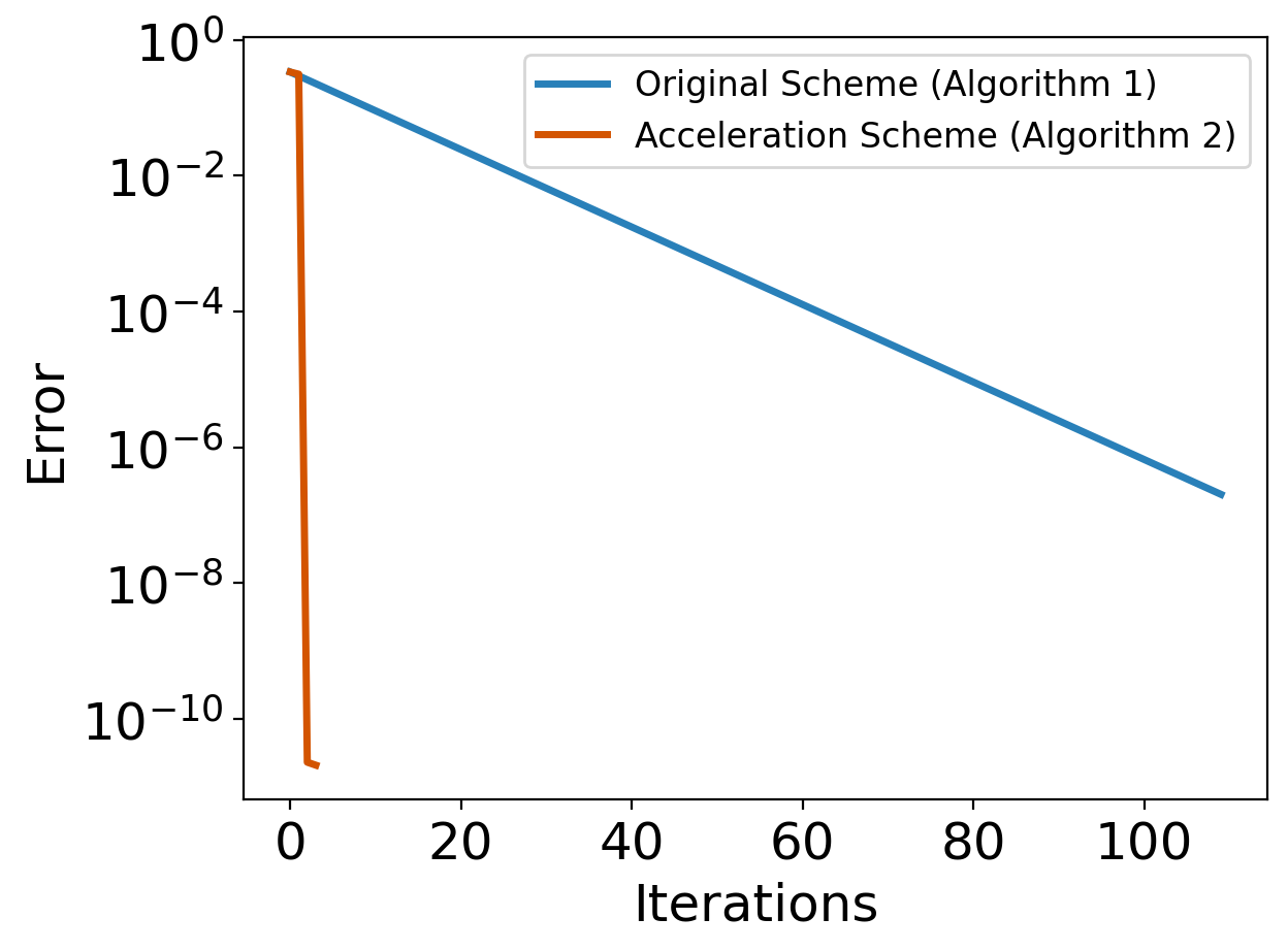
(a) Iteration difference:
$\|F-F_{\mathcal{G}}-F_{\mathcal{H}}\|$

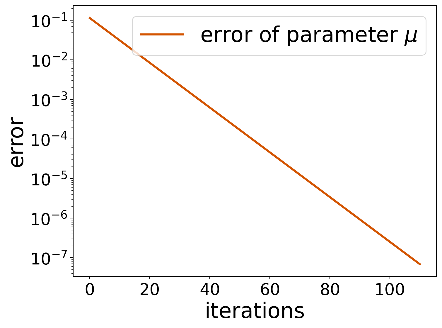
(b) Error of parameter:
$\|\mu-\mu_{\mathrm{ref}}\|$

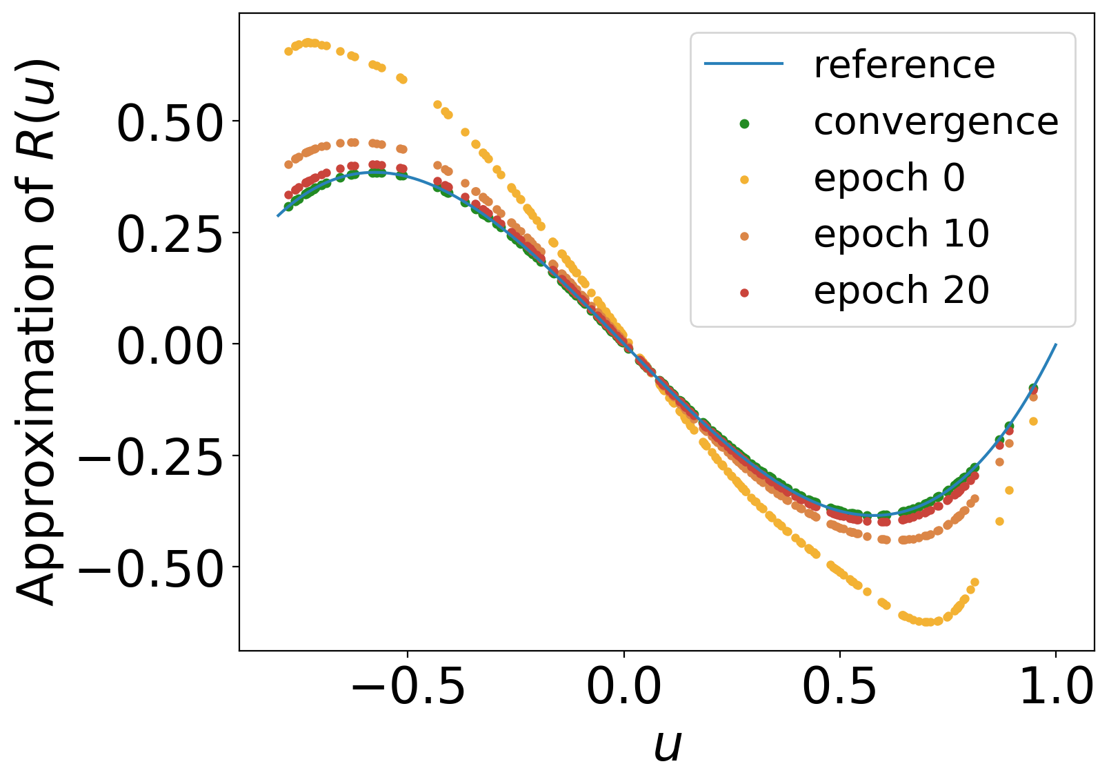
(c) Convergence trajectory
of $R(u)$

Figure 3: Convergence trajectory of reaction-diffusion

For the long-time prediction evaluation, we randomly select 50 initial points $u_{0}$ and predict their evolution over 50 time steps using our iterative model combination algorithm. We then compare the performance of our scheme with two other methods: using Koopman operator approach with the same dictionary alone, and a residual-learning approach that involves conducting linear regression first and then using the Koopman operator for correction. In figure 4, the lines represent the average error of the 50 predicted trajectories, while the shaded areas represent the standard deviation of the estimates. Here, the error is defined as

$$\mathrm{error}_{k}=\frac{\|u_{k}^{\mathrm{predict}}-u_{k}^{\mathrm{ref}}\|}{\|u^{\mathrm{ref}}\|},$$ (33)

where $u_{k}^{\mathrm{predict}}$ represents predicted values at the $k$-th time step, and $u_{k}^{\mathrm{ref}}$ represents simulation values at the $k$-th time step. $u^{\mathrm{ref}}$ is constructed as $[u_{0}^{\mathrm{ref}},u_{1}^{\mathrm{ref}},u_{2}^{\mathrm{ref}},\ldots,u_{50}^{\mathrm{ref}}]$. Figure 4 demonstrates that combination of Koopman operator and linear regression methods can have better accuracy than baselines in prediction problems.

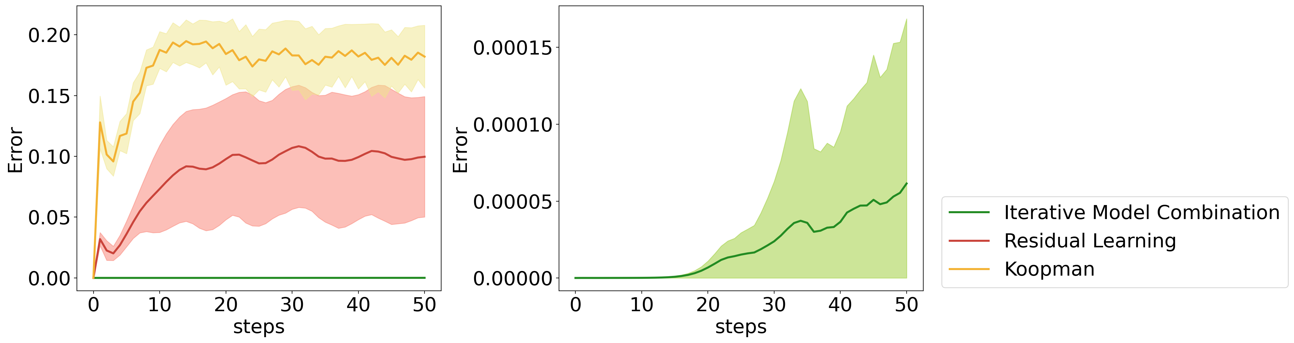
Figure 4: Long-time prediction of the reaction-diffusion solution

Table 1 shows the relative error of four methods over the prediction domain, which is the discretization of

$$e_{\Omega\times[t_{1},t_{2}]}=\frac{\sum_{(z,t)\in\Omega\times[t_{1},t_{2}]}\|u^{\mathrm{predict}}(z,t)-u^{\mathrm{ref}}(z,t)\|}{\sum_{(z,t)\in\Omega\times[t_{1},t_{2}]}\|u^{\mathrm{ref}}(z,t)\|}.$$ (34)

In our experiment, $\Omega=[0,1]$, $t_{1}=0$, and $t_{2}=0.05$. Table 1 shows that both the Koopman model and the linear model perform poorly when used individually. The introduction of residual learning results in some accuracy improvement, but is still sub-optimal. In contrast, our method significantly outperforms the baselines by a few orders of magnitude.

	Relative Error
Linear regression	17724.6914%
Koopman Operator	115.6717%
Residual learning	65.7356%
Iterative hybrid modelling	0.0761%

Table 1: Relative error over the prediction domain $[0,1]\times[0,0.05]$

4.3 Cardiac electrophysiology model

Problem

Data-driven modelling of partially-known dynamical systems is a common task in science and engineering. One example is a PDE-ODE coupled system in cardiac electrophysiology [34, 35]:

$$\begin{split}v_{t}-\nabla\cdot(\Lambda\nabla v)&=I_{s}-I_{ion}(v,s)\quad\mathrm{in}\ \Omega\times(0,T),\\ s_{t}&=F(v,s)\quad\mathrm{in}\ \Omega\times(0,T).\end{split}$$ (35)

Here, the transmembrane potential $v$ is a one-dimensional variable, and $s$ is a three-dimensional one, representing the gating variable of currents. $\Lambda$ is the conductivity tensor of the mono-domain equation and $I_{s}$ is a given stimulus current. The term $I_{ion}$ is the ionic current describing a response of the cardiac cell with the gating variable $s(z,t)$ which evolves according to (35). The functions $I_{ion}$ and $F$ are specific to a given cell model as they describe the cell’s dynamics. However, understanding which properties of the cell are relevant for its electrical behavior and how these properties interact is a challenging problem. According to [5], it is thus reasonable to consider a setting where $F$ and $I_{ion}$ would be learned from data of a specific patient. Researchers have explored the use of neural networks to approximate the unknown components and integrate them with the incomplete physics model in partially-known systems [5]. However, these methods rely on the careful design of a physical model, particularly in (35), where the accurate selection of the matrix $\Lambda$ is essential. Instead of fixing it in advance, we choose it adaptively using Algorithm 1. Thus, in this experiment, we suppose the matrix $\Lambda$ and the functions $I_{\mathrm{ion}}(v,s)$ and $F(v,s)$ are unknown. The objective is to predict the trajectory of $v$ and $s$ accurately with new stimulus $I_{s}$.

Methods

We choose two models with hypothesis spaces $\mathcal{G}$, $\mathcal{H}$ according to properties of this specific problem: one as linear regression of fusion terms

$$\begin{split}\mathcal{G}:F_{\mathcal{G}}(x(z_{i,j},t_{k}))=[\mu_{1}\frac{v(z_{i+1,j},t_{k})+v(z_{i-1,j},t_{n})-2v(z_{i,j},t_{n})}{(\Delta z)^{2}}\\ +\mu_{2}\frac{v(z_{i,j+1},t_{k})+v(z_{i,j-1},t_{k})-2v(z_{i,j},t_{k})}{(\Delta z)^{2}},0,0,0]^{T},\end{split}$$ (36)

another as Parametric Koopman Operator [22]

$$\mathcal{H}:F_{\mathcal{H}}(x(z_{i,j},t_{k}))=g\circ K(I_{s}(z_{i,j},t_{k}))\Psi(y(z_{i,j},t_{k})),$$ (37)

where $x(z_{i,j},t_{k})=[v(z_{i,j},t_{k}),s(z_{i,j},t_{k})]$ and $g$ is the function used to extract states from the dictionary.

To obtain the representation of the operator $K(I_{s})$, we construct a ResNet [36] $NN_{K}(I_{s})$, comprising two hidden layers, each with 32 nodes. The input of $NN_{K}(I_{s})$ is the stimulus, and the output consists of the elements of the matrix $K(I_{s})$. Subsequently, we reshape the output of the neural network to obtain the matrix $K(I_{s})$. Additionally, we utilize a trainable dictionary [21] in our experiments. The dictionary is constructed using a ResNet denoted as $NN_{\Psi}(x)$, which consists of 2 hidden layers, each with 64 nodes. The input of $NN_{\Psi}(x)$ is the state of dynamics $x$, and the output is a group of observables of $x$. We construct the dictionary $\Psi(x)$ as

$$\Psi(x)=[1,x,NN_{\Psi}(x)].$$ (38)

In our experiment, the dictionary $\Psi(x)$ has a total dimension of 27. The structures of neural networks are illustrated in figure 5. In this experiment, we let $\Omega=[10]^{2}$ and $T=5$. The domain $\Omega$ is discretized with a mesh size $\Delta z=0.2$, and we simulate the coupled system using a time step $\Delta t=0.2$. For the training data, we define the inputs $I_{s}$ as follows:

$$I_{s}(z,t)=d(z_{1},z_{2})\sin(t),$$ (39)

where $d(z_{1},z_{2})=z_{1}+10-z_{2}$. During the training process, we initially perform pre-training on the dictionary network $NN_{\Psi}(x)$ and freeze the parameters in $NN_{\Psi}(x)$. Subsequently, we iteratively optimize the parameters $\mu_{1}$ and $\mu_{2}$ using linear regression and train the operator network $NN_{K}(I_{s})$ using the Adam optimizer. In this experiment, due to the nonlinear structure of operator network $NN_{K}(I_{s})$, it is no longer a linear problem as before.

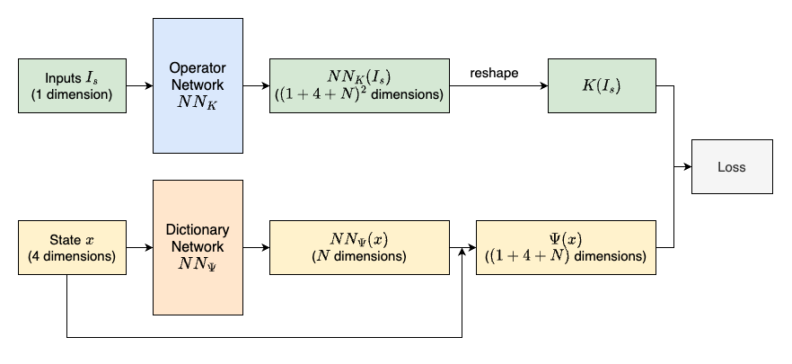
Figure 5: Structure of the parametric Koopman model

Results

Figure 6 shows the convergence patterns of our schemes. We observe that initially the iteration error decreases rapidly. However, since the neural networks for the Koopman operator could only obtain an approximate projection $P_{\mathcal{H}}(F-F_{\mathcal{G}})$, the error exhibits slight fluctuations thereafter. Also, the acceleration scheme (Algorithm 2) has faster convergence than the original scheme (Algorithm 1). Furthermore, the relative error of parameters decreases to less than 10% within a few epochs.

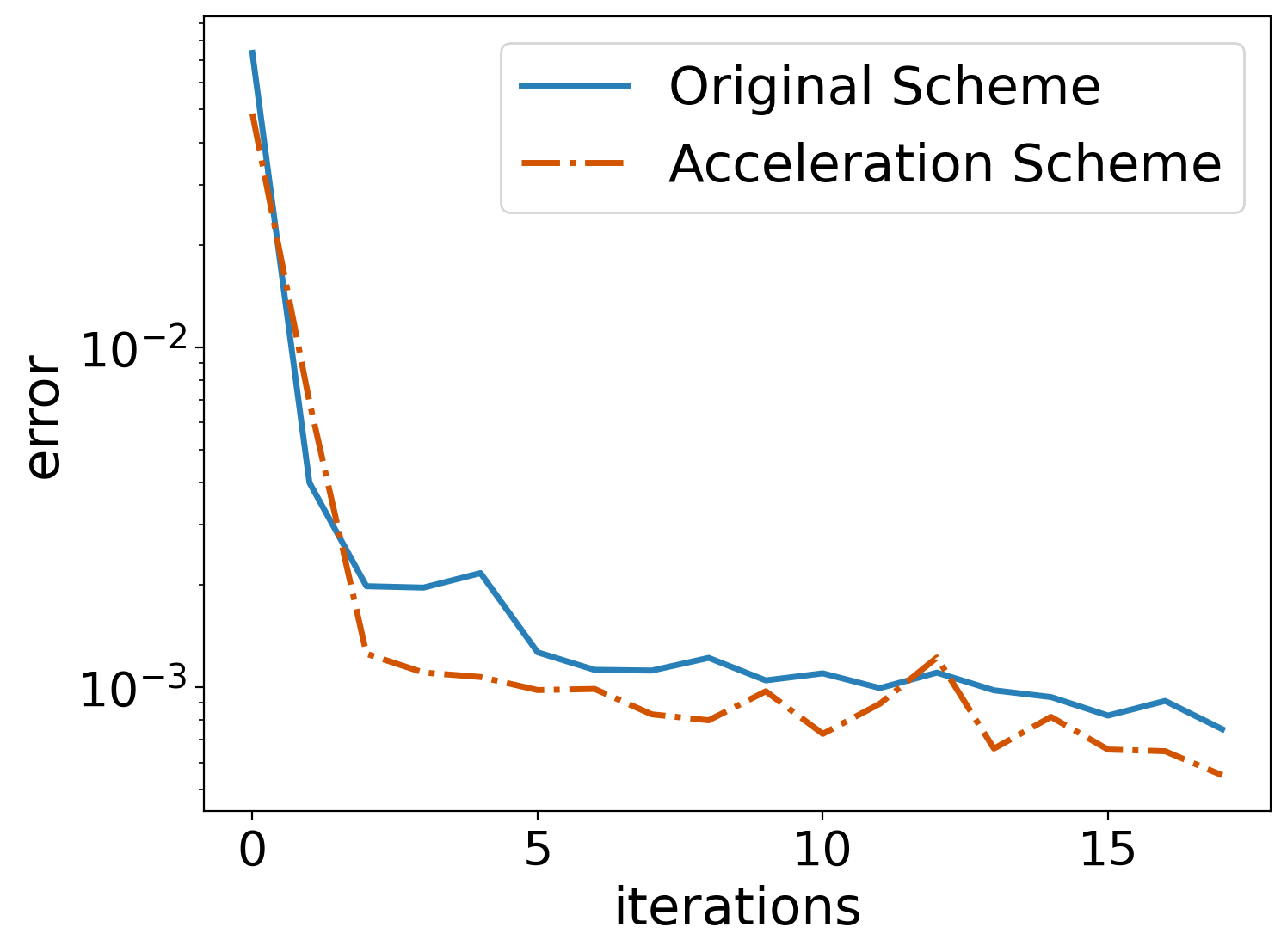
(a) Iteration difference:
$\|F-F_{\mathcal{G}}-F_{\mathcal{H}}\|$

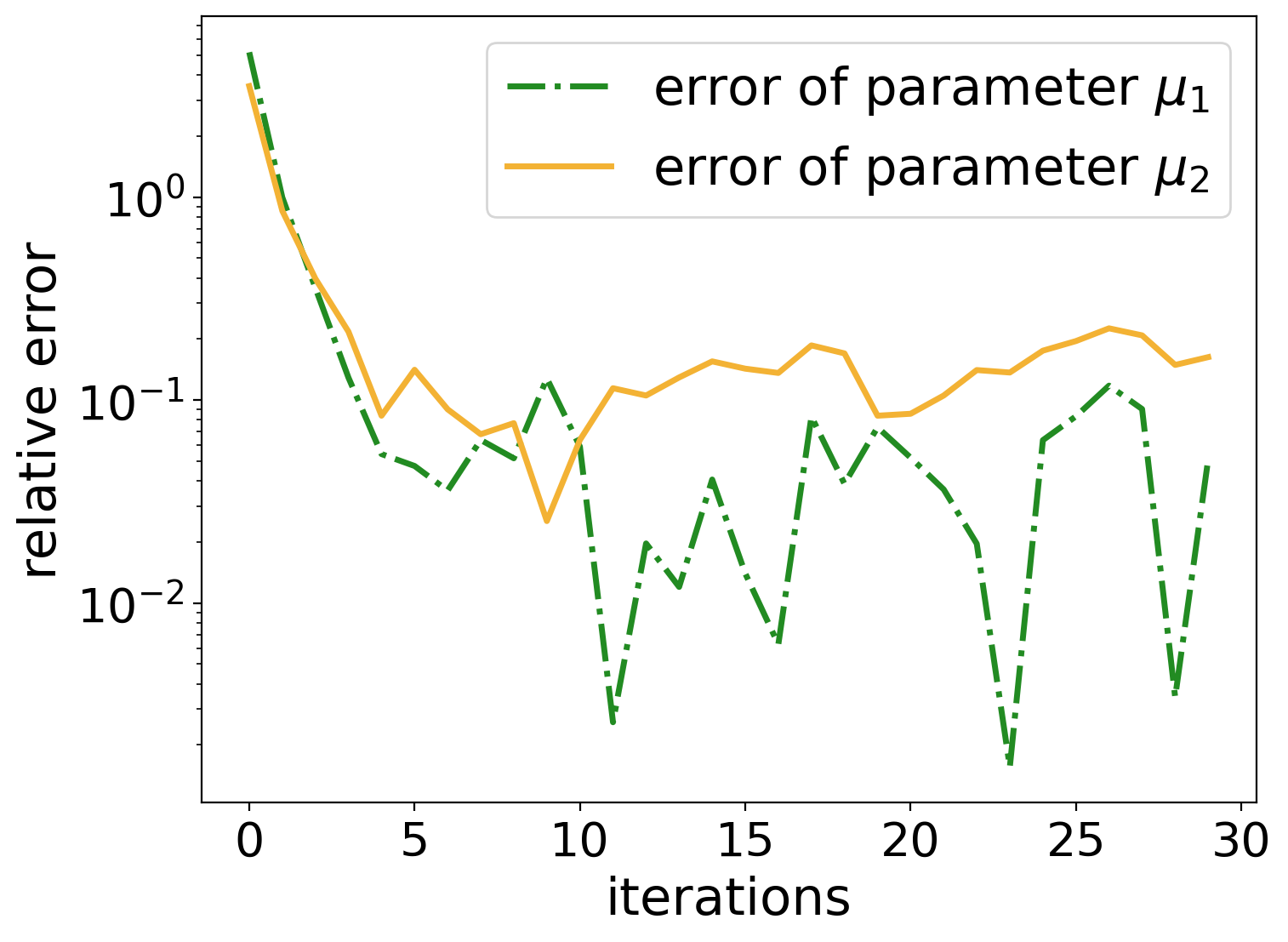
(b) Error on parameter:
$\|\mu-\mu_{\mathrm{ref}}\|$

Figure 6: Convergence trajectory of the cardiac model

The predicted states are depicted in figure 7. These predictions utilize the same initial conditions and external stimulus as those employed during training. We chose the spatial coordinates $z=(2.8,9.8)$ to present the predicted results because the system trajectory exhibits significant nonlinearity at this point. We plot the predicted states at the spatial coordinates $z=(2.8,9.8)$ in the top figures. Both the transmembrane potential $v$ and the gating variable $s$ closely approximate the reference values. Furthermore, the spatial distribution of the transmembrane potential $v$ at $t=3$ demonstrates the superior performance of our methods compared to using the parametric Koopman model alone. Quantitatively, the relative error, defined in (34), in $\Omega\times[0,3]$ of the transmembrane potential $v$ and the gating variable $s$ is shown in table 2. In this case, the multi-step predictive states of linear regression strictly equal the initial conditions, as the initial conditions for $v$ and $s$ over the spatial domain $\Omega$ are chosen to be constant. Furthermore, since the iteration scheme in model combination employs the forward-Euler scheme of a dynamical system, which is not unconditionally stable, the residual learning in this experiment is significantly affected by stiffness, causing the error to explode after a few steps. When comparing our method to the parametric Koopman model, we can observe a significant performance improvement in our approach.

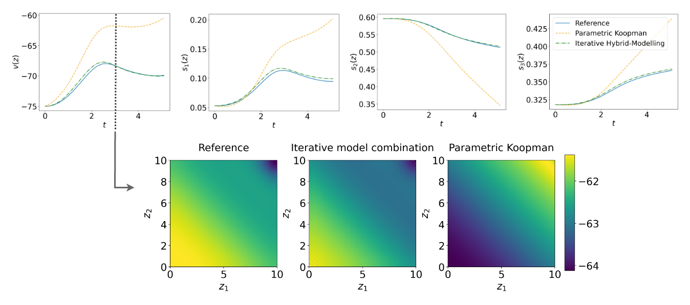
Figure 7: Predicted states with same initial conditions and external stimulus. Top: Predicted states at spatial coordinates $z=(2.8,9.8)$. Bottom: Spatial distribution of the transmembrane potential $v$ at $t=3$. Left: the reference distribution; Middle: by iterative model combination algorithm; Right: by Parameterized Koopman.

	$v$	$s_{1}$	$s_{2}$	$s_{3}$
Linear regression	10.4159%	58.5347%	8.2891%	8.2365%
Parametric Koopman Model	4.3523%	13.4181%	3.0881%	1.9963%
Residual learning	$\geq 100\%$	$\geq 100\%$	$\geq 100\%$	$\geq 100\%$
Iterative model combination algorithm	0.3269%	1.6881%	0.5201%	0.2469%

Table 2: Relative error of prediction in $\Omega\times[0,3]$ with same initial conditions and external stimulus

We also tested the models with a new stimulus, denoted as $I_{s}(z,t)=d(z_{1},z_{2})\cos(t)$. Figure 8 displays the predicted state at the spatial coordinates $z=(2.8,9.8)$ and predicted spatial distribution at $t=2$, illustrating our method’s capability to handle previously unseen inputs. Quantitatively, table 3 presents the relative errors, defined in (34), in $\Omega\times[0,2]$ for both the transmembrane potential $v$ and the gating variable $s$ with different external stimuli. We can observe that the results are similar to the predictive experiment with the same external stimulus, emphasizing that our method can also exhibit better performance when faced with unseen stimuli.

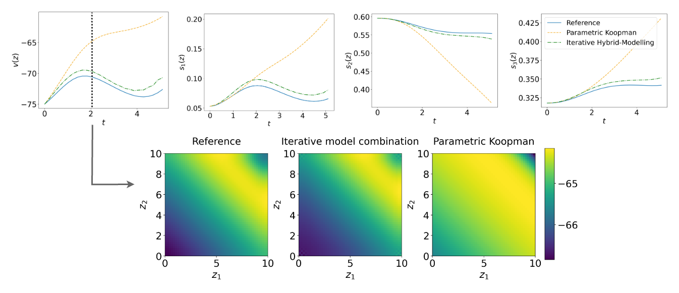
Figure 8: Predicted states with different external stimuli. Top: Predicted states at spatial coordinates $z=(2.8,9.8)$. Bottom: Spatial distribution of the transmembrane potential $v$ at $t=2$. Left: the reference distribution; Middle: by hybrid-modelling; Right: by Parameterized Koopman.

	$v$	$s_{1}$	$s_{2}$	$s_{3}$
Linear regression	7.8192%	49.9801%	7.1977%	7.1436%
Parametric Koopman Model	8.5179%	25.4762%	4.9132%	3.3072%
Residual learning	$\geq 100\%$	$\geq 100\%$	$\geq 100\%$	$\geq 100\%$
Iterative model combination algorithm	0.9913%	7.7024%	0.3785%	0.8246%

Table 3: Relative error of prediction in $\Omega\times[0,2]$ with different external stimuli.

4.4 Model predictive control in parameterized systems

Problem

In this section, we consider a parameterized discrete-time nonlinear controlled dynamical system

$$x_{n+1}=F(x_{n},c_{n},e_{n}),$$ (40)

where $x_{n}\in X\subset\mathbb{R}^{K}$ denotes the state of the system, $c_{n}\in\mathcal{C}\subset\mathbb{R}^{m_{c}}$ is the control input, $e_{n}\in\mathcal{E}\subset\mathbb{R}^{m_{e}}$ represents the external input, and $F$ is the transition mapping. The control input $c_{n}$ remains subject to adjustments and monitoring by the controller, whereas $e_{n}$ is influenced by external factors and cannot be controlled.

An example for such control problem is the dynamics of a robotic fish studied in [37]. The states of the robotic fish are $s=[x,y,\phi,v_{x},v_{y},\omega]^{T}$, where $x,y$ are the world-frame coordinates, $\phi$ is the orientation, $v_{x}$ and $v_{y}$ are the body-frame linear velocities (surge and sway, respectively), and $\omega$ is the body-frame angular velocity. We use $\alpha$ to indicate the angle of the tail. The tail is actuated with $\alpha(t)=\alpha_{0}+\alpha_{a}\sin(\omega_{a}t)$, where $\alpha_{a},\alpha_{0},\omega_{a}$ are the amplitude, bias, and frequency of the tail beat. We use the bias $\alpha_{0}$ and amplitude $\alpha_{a}$ as control inputs, while the frequency $\omega_{a}$, which may be determined by battery and mechanical constraints, will be used as an external input in the simulation. The dynamical system is defined as an average model for tail-accurate systems [38]:

$$\dot{s}=\left[\begin{array}[]{c}\dot{x}\\ \dot{z}\\ \dot{\psi}\\ \dot{v}_{x}\\ \dot{v}_{y}\\ \dot{\omega}\end{array}\right]=F(s)\triangleq\left[\begin{array}[]{c}v_{x}\cos(\psi)-v_{y}\sin(\psi)\\ v_{x}\sin(\psi)+v_{y}\cos(\psi)\\ \omega\\ f_{1}(s)+K_{f}f_{4}\left(\alpha_{0},\alpha_{a},\omega_{a}\right)\\ f_{2}(s)+K_{f}f_{5}\left(\alpha_{0},\alpha_{a},\omega_{a}\right)\\ f_{3}(s)+K_{m}f_{6}\left(\alpha_{0},\alpha_{a},\omega_{a}\right)\end{array}\right]$$ (41)

with detailed information of parameters and functions in [37].

We focus on the tracking problem with (41). The problem is formulated as follows: given the initial value $s_{0}$ and external inputs $\{w_{i}\}$, we would like to obtain a sequence of controlled inputs $\{c_{i}\}$ minimizing $\sum_{i=1}^{n}((s_{i}-s^{\mathrm{ref}}_{i})^{T}Q(s_{i}-s^{\mathrm{ref}}_{i})+c_{i}^{T}Rc_{i})$ where $s_{i+1}=f(s_{i},c_{i},e_{i})$ and $Q,R$ are semi-positive matrices. We solve this tracking problem by Model Predictive Control (MPC) where the current control is obtained by solving a finite horizon open-loop optimal control problem at each sampling instant. The MPC formulation solves the following optimization problem:

$$\min_{c_{0},c_{1},\ldots,c_{h-1}}J(z,c,e)$$ (42)

$$\text{s.t.}\quad z_{i}=\hat{f}(z_{i-1},c_{i-1},e_{i-1})$$

$$c_{i-1}\in[a_{i-1},b_{i-1}]$$

where $J(z,c)=\sum_{i=1}^{h}(z_{i}-z^{ref}_{i})^{T}Q(z_{i}-z^{ref}_{i})+\sum_{i=1}^{h}{c_{i}}^{T}Rc_{i}$. The MPC solver is outlined in Algorithm 3. For more information on the MPC method, the reader may consult the review [39].

Algorithm 3 MPC solver in parameterized dynamical system

Initial value $x_{0}$, dictionary $\Psi$, horizon length $h$, trajectory length $N$, reference trajectory $\mathbf{x}^{\mathrm{ref}}$, external inputs $\mathbf{\hat{c}}$

$z_{0}\leftarrow\Psi(x_{0})$

$\mathbf{z}^{\mathrm{ref}}=\Psi(\mathbf{x}^{\mathrm{ref}})$

for $i=1$ to $N$ do

     Solve the open-loop optimal control problem from $i$ to $i+h$ steps

     $c_{i}\leftarrow\text{OptimalControlSolver}(z_{i-1},i,h,\mathbf{z}^{\mathrm{ref}}[i,i+h])$ $\triangleright$ Solve optimization problem

     Propagate state: $x_{i}\leftarrow F(x_{i-1},c_{i},e_{i})$ $\triangleright$ Update state using dynamics

     $z_{i}\leftarrow\Psi(x_{i})$

end for

The fundamental challenge in an MPC solver lies in selecting the appropriate transition function of observables, denoted as $z_{i+1}=\hat{f}(z_{i})$ in Algorithm 3. Unlike the previous two experiments, in this section we compare the models with different structures for solving the control problem, highlighting the fact that our method of model combination can provide more accurate solutions when dealing with the control problem and guarantee the convexity of the optimization problem.

Methods

Some data-driven methods are proposed for the linearization of the MPC problem. Two representative structures are a linear structure [23] as $z_{n+1}=Kz_{n}+Bc_{n}$ and nonlinear structure [15, 22] as $z_{n+1}=K(c_{n})z_{n}$. Given that the control is on $c$, our model combination strategy can ensure that the dynamics is linear in $c$ while a nonlinear structure is used to handle the external input $e$. We express this as follows:

$$z_{n+1}=K(e_{n})z_{n}+Bc_{n}.$$ (43)

Another approach to merging these two structures is represented by:

$$z_{n+1}=Kz_{n}+B(e_{n})c_{n},$$ (44)

as $c_{n}$ could also be treated as part of the dictionary.

Thus, we compare the performance of the following four structures, where only the hybrid ones are trained using the proposed method:

• Linear structure, similar to [23]: $z_{n+1}=K_{1}z_{n}+B_{1}c_{n}+C_{1}e_{n}$,

• Hybrid structure (our methods, represented as hybrid structure 1 and hybrid structure 2 respectively):

  • $z_{n+1}=K_{2}(e_{n})z_{n}+B_{2}c_{n}$,

  • $z_{n+1}=K_{3}z_{n}+B_{3}(e_{n})c_{n}$,

• Nonlinear structure, similar to [15, 22]: $z_{n+1}=K_{4}(e_{n},c_{n})z_{n}$.

The optimization problem in (42) with linear and hybrid structures is convex, with a guarantee in obtaining an optimal solution, whereas with nonlinear structure it is non-convex. We parametrize the observables using a fully-connected neural network denoted as $NN_{\Psi}(s)$, and establish the dictionary as $\Psi(s)=[1,s,NN_{\Psi}(s)]$. The dimension of the dictionary $\Psi(s)$ is randomly picked as 25 in this experiment.

Throughout our experiments, we follow a two-step process: initially, we perform pre-training to learn the dictionary and subsequently fix it; then, we proceed to train the operators. The traditional Koopman operator ($K_{1},B_{1},C_{1},B_{2},K_{3}$) is computed via least squares, while the parameterized Koopman operator ($K_{2}(e),B_{3}(e),K_{4}(c,e)$) is constructed using a fully connected neural network. In the case of the hybrid structure, we use the Adam optimizer to train the parameterized operator network for 5 epochs and perform a least squares update on the traditional Koopman operator by Algorithm 1. This process is repeated for a total of 200 iterations. On the other hand, for the nonlinear structure, we train the operator network for 1000 epochs.

To generate data, we sample $P=1000$ initial conditions for the states with uniform distributions given by table 4. For each individual sample, we apply random inputs generated from uniform distributions: $U_{\alpha_{0}}\left(-50^{\circ},50^{\circ}\right)$ for the tail angle bias, $U_{\alpha_{a}}\left(0,30^{\circ}\right)$ for the tail angle amplitude of oscillations, and $U_{\omega_{a}}\left(0,10\pi\ \mathrm{rad/s}\right)$ for the frequency. Then, for each specific combination of initial conditions $s_{k}$, controlled inputs $u_{k}$, and external inputs $w_{k}$, we employ the dynamics described in (41), we generate data for a total of 50 discrete time steps with a time step $\Delta t=1\mathrm{s}$. Additionally, for the tracking problem, we construct the reference trajectory using constant inputs: $\alpha_{0}=\frac{1}{6}\pi$, $\alpha_{a}=\frac{1}{18}\pi$, and $\omega_{a}=2\pi$. Subsequently, we leverage the linear, hybrid, and nonlinear structures to track the trajectory under distinct external input conditions for $\omega_{a}$, which are set to $2\pi$, $2\pi+\pi\sin(\frac{\pi}{60}t)$, and random samples uniformly selected in $[0,10\pi]$, respectively. In the MPC problem, we choose the horizon length and cost function as follows: $h=5$, $Q=\mathrm{diag}\{0,0,0,0,10^{8},0.01,10^{8},0,\ldots,0,\ldots\}$, $R=\mathrm{diag}\{0.1,0.1\}$ and the total length of trajectory is 180. The optimization problems are solved by the L-BFGS-B method.

Parameter	Distribution
$x$	$\mathcal{U}(-0.5,0.5)$
$y$	$\mathcal{U}(-0.1,0.1)$
$\phi$	$\mathcal{U}(-\pi/4,\pi/4)$
$v_{x}$	$\mathcal{U}(0,0.04)$
$v_{y}$	$\mathcal{U}(-0.0025,0.0025)$
$\omega$	$\mathcal{U}(-0.5,0.5)$

Table 4: Distribution of initial values

Results

The results of the tracking experiment are visually depicted in figure 9. In the tracking problem described in the previous paragraph, we are primarily concerned with only two dimensions, namely $v_{x}$ and $\omega$ (the 5th and 7th dimensions of $\Psi(s)$), as they play a crucial role in maintaining the shape of the robotic fish’s trajectory. The figure on the left displays the mean tracking error of $v_{x}$ and $\omega$, which is defined as:

$$\text{mean tracking error}=\frac{1}{2}\left(\frac{\max_{i}|v_{x}(t_{i})-v_{x}^{\text{ref}}(t_{i})|}{\max_{i}|v_{x}^{\text{ref}}(t_{i})|}+\frac{\max_{i}|\omega(t_{i})-\omega^{\text{ref}}(t_{i})|}{\max_{i}|\omega^{\text{ref}}(t_{i})|}\right).$$ (45)

Additionally, the computation time of the MPC problem is shown on the right. The linear structure has the benefit of simplicity and the fastest solving time. However, when the external inputs $\omega_{a}$ change rapidly (e.g., when $\omega_{a}$ is chosen randomly), the predicted trajectory exhibits significant oscillations. The nonlinear structure is sometimes susceptible to optimization errors and exhibits poor accuracy even in simple problem settings. In comparison to these two, our methods demonstrate good performance with a modest time cost.

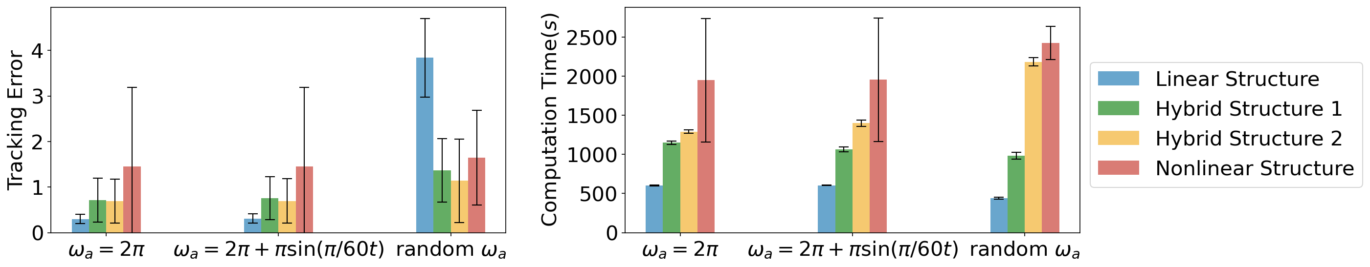
Figure 9: Tracking problem for different external inputs $\omega_{a}$. Left: mean tracking error of $v_{x}$ and $\omega$. Right: computation time of the MPC problem.

5 Conclusion

Model combination holds significant potential in modelling high-dimensional and complex dynamical systems. In this paper, we introduced a linearly convergent iterative model combination algorithm, an approach that efficiently combines two model spaces through addition in a non-intrusive way. We provided both theoretical and empirical evidence to support its convergence patterns. Furthermore, our numerical experiments confirm the effectiveness of our approach in addressing both prediction and control problems within complex systems. In future studies, it would be interesting to explore extending our method to incorporate unsupervised learning for model selection and acceleration strategies, and to apply the methodology on engineering cases of interest.

Appendix A Proof

A.1 Proof of theorem 1

Lemma 1 (Von Neumann [27]).

Set $b_{0}:=x,a_{n}:=P_{A}(b_{n-1}),b_{n}:=P_{B}(a_{n})$. We claim that both $\{a_{1},a_{2},a_{3},...,a_{n},...\}$ and $\{b_{0},b_{1},b_{2},...,b_{n},...\}$ will converge to $P_{A\cap B}(x)$ in norm whenever $A,B$ are closed subspaces.

Proof.

For $b_{k}=P_{B}(a_{k})$, we have $(a_{k}-b_{k})^{T}\cdot b_{k}=0.$ Then

$$\begin{split}\|a_{k}\|^{2}=\|a_{k}-b_{k}+b_{k}\|^{2}\\ =\|a_{k}-b_{k}\|^{2}+\|b_{k}\|^{2}+2(a_{k}-b_{k})^{T}\cdot(b_{k})\\ =\|a_{k}-b_{k}\|^{2}+\|b_{k}\|^{2}.\end{split}$$ (46)

Then $\|b_{k}\|^{2}\leq\|a_{k}\|^{2}.$
Similarly, we could prove $\|a_{k+1}\|\leq\|b_{k}\|\leq\|a_{k}\|\leq\|b_{k-1}\|\leq...\leq\|x\|.$ Both $\{\|b_{k}\|\}$ and $\{\|a_{k}\|\}$ are non-increasing sequences, and converge to $B,A$.
For a bounded sequence $\{a_{k}\}$, there exists a subsequence $\{a_{k_{i}}\}$ such that

$$a_{k_{i}}\to\hat{x}\quad\mathrm{as}\ k_{i}\to+\infty.$$ (47)

From (46), we have $\|a_{k}-b_{k}\|\to 0$ as $k\to+\infty,$ then

$$\mathrm{dist}(a_{k_{i}},B)\leq\mathrm{dist}(a_{k_{i}},b_{k_{i}})\to 0\quad\mathrm{as}\ k_{i}\to+\infty.$$ (48)

Thus, $\hat{x}\in B$. Since $A$ is closed, $\hat{x}\in A\cap B.$
For $b_{k}=P_{B}(a_{k})$, we have $(a_{k}-b_{k})^{T}\cdot(b_{k}-\hat{x})=0.$ Then

$$\begin{split}\|a_{k}-\hat{x}\|^{2}=\|a_{k}-b_{k}+b_{k}-\hat{x}\|^{2}\\ =\|a_{k}-b_{k}\|^{2}+\|b_{k}-\hat{x}\|^{2}+2(a_{k}-b_{k})^{T}\cdot(b_{k}-\hat{x})\\ =\|a_{k}-b_{k}\|^{2}+\|b_{k}-\hat{x}\|^{2}.\end{split}$$ (49)

Then $\|a_{k}-\hat{x}\|\to 0$, $\|b_{k}-\hat{x}\|\to 0$ as $k\to+\infty.$
We only need to illustrate $\hat{x}=P_{A\cap B}(x).$
Separate $x$ into two terms

$$x=P_{A\cap B}(x)+(I-P_{A\cap B})(x),$$ (50)

we observe that $P_{A}P_{A\cap B}=P_{A\cap B}P_{B}$, then when repeating the projection to $A$ and $B$,

$$a_{k}=P_{A\cap B}(x)+(I-P_{A\cap B})(a_{k})\to P_{A\cap B}(x)\quad\mathrm{as}\ k\to+\infty,$$ (51)

that is, $\hat{x}=P_{A\cap B}(x).$ ∎

Proof of Theorem 1

Proof.

1. Let $n=1$,

   $$\begin{split}[(I-P_{\mathcal{G}})\circ(I-P_{\mathcal{H}})](F)&=(I-P_{\mathcal{G}}-P_{\mathcal{H}}+P_{\mathcal{G}}P_{\mathcal{H}})(F)\\ &=F-P_{\mathcal{G}}(I-P_{\mathcal{H}})(F)-P_{\mathcal{H}}(F)\\ &=F-P_{\mathcal{G}}(I-P_{\mathcal{H}})(F)+F_{H}^{1}\\ &=F-P_{\mathcal{G}}(F-F_{H}^{1})-F_{H}^{1}\\ &=F-F_{G}^{1}-F_{H}^{1}.\end{split}$$ (52)

   Suppose that when $n=k$, $[(I-P_{\mathcal{G}})\circ(I-P_{\mathcal{H}})]^{k}(F)=F-F_{\mathcal{G}}^{k}-F_{\mathcal{H}}^{k}$, then we have

   $$\begin{split}[(I-P_{\mathcal{G}})\circ(I-P_{\mathcal{H}})](F-F_{G}^{k}-F_{H}^{k})\\ =F-F_{G}^{k}-F_{H}^{k}-P_{\mathcal{G}}(I-P_{\mathcal{H}})(F-F_{G}^{k}-F_{H}^{k})-P_{\mathcal{H}}(F-F_{G}^{k})+F_{H}^{k}\\ =F-F_{G}^{k}-F_{H}^{k}-P_{\mathcal{G}}(F-F_{G}^{k}-F_{H}^{k+1})-F_{H}^{k+1}+F_{H}^{k}\\ =F-F_{G}^{k+1}-F_{H}^{k+1}\end{split}$$ (53)

   Let $A=\mathcal{G}^{\bot},B=\mathcal{H}^{\bot},b_{0}=F$ in Lemma 1,

   $$\begin{split}\lim_{n\to+\infty}\|P_{\mathcal{G}\oplus\mathcal{H}}(F)-F_{G}^{n}-F_{H}^{n}\|\\ =\lim_{n\to+\infty}\|(I-P_{\mathcal{G}\oplus\mathcal{H}})(F)-[(I-P_{\mathcal{G}})\circ(I-P_{\mathcal{H}})]^{n}(F)\|=0.\end{split}$$ (54)

2. Let $\{\tilde{x}_{k}\}$ be the trajectory generated by $\tilde{x}_{k+1}=P_{\mathcal{G}\oplus\mathcal{H}}(\hat{x}_{k})$ and $\tilde{F}=P_{\mathcal{G}\oplus\mathcal{H}}(F)$. $\forall k$,

   $$\begin{split}\epsilon_{k}=\|\tilde{x}_{k}-x_{k}^{n}\|&\leq\|\tilde{F}(\tilde{x}_{k-1})-F^{n}(\tilde{x}_{k-1})\|+\|F^{n}(\tilde{x}_{k-1})-F^{n}(x_{k-1}^{n})\|\\ &\leq\|\tilde{F}-F^{n}\|\|\tilde{x}_{k-1}\|+\|F^{n}\|\epsilon_{k-1}\end{split}$$ (55)

   Since $\epsilon_{0}=0$, $\epsilon_{1}\leq\|\tilde{F}-F^{n}\|\|\tilde{x}_{0}\|\to 0$. Let $\|\tilde{x}_{k-1}\|=M_{k-1}$. Then, $\forall\epsilon>0,\exists N_{1}>0$, such that

   $$\forall n>N_{1}\quad\|\tilde{F}-F^{n}\|\leq\frac{\epsilon}{2M_{k-1}}.$$ (56)

   $\exists N_{2}>0$, such that

   $$\epsilon_{k-1}<\epsilon/2(\frac{\epsilon}{2M_{k-1}+1+\epsilon_{F}}).$$ (57)

   Thus, set $N=\max\{N_{1},N_{2}\}$, we have

   $$\epsilon_{k}<\frac{\epsilon}{2}+\frac{\epsilon}{2}<\epsilon,$$ (58)

   the trajectory $\{x^{n}_{k}\}$ generated by $x^{n}_{k+1}=F^{n}(x^{n}_{k})$ with $x^{n}_{0}=x_{0}$ will converge to a sequence $\{\tilde{x}_{k}\}$.
   For the distance from $\{\tilde{x}_{k}\}$ to $\{x_{k}\}$, we have

   $$\begin{split}e_{k}=\|\tilde{x}_{k}-x_{k}\|&=\|\tilde{F}(\tilde{x}_{k-1})-\tilde{F}(x_{k-1})\|+\|\tilde{F}(x_{k-1})-F(x_{k-1})\|\\ &\leq(1+\epsilon_{F})e_{k-1}+\epsilon_{F}M.\end{split}$$ (59)

   Since $e_{0}=0$,

   $$e_{k}\leq((1+\epsilon_{F})^{k}-1)M.$$ (60)

   Specifically, if $F\in\mathcal{H}\oplus\mathcal{G}$, $\epsilon_{F}$ = 0, then $e_{k}=0$, $e^{n}_{k}=\epsilon^{n}_{k}\to 0$ as $n\to+\infty$.

∎

A.2 Proof of theorem 2

Lemma 2.

[40]

$$c_{0}(A,B)=\|P_{A}P_{B}\|$$ (61)

Proof.

for $y=P_{B}(F)$,

$$|\langle P_{A}(y),y\rangle|=\|P_{A}(y)\|\|P_{A}P_{B}(y)\|=\|P_{A}P_{B}(y)\|^{2}\leq c_{0}(A,B)\|P_{A}(y)\|\|y\|,$$ (62)

then

$$\|P_{A}P_{B}(y)\|\leq c_{0}(A,B)\|y\|.$$ (63)

For $y\in B$, we have that

$$P_{A}(y)=\mathrm{argmin}_{F\in A}\frac{|\langle F,y\rangle|}{\|F\|\|y\|}.$$ (64)

For $A,B$ some closed subspaces, there exists $y_{0}\in B$ such that

$$c(A,B)=\frac{|\langle P_{A}(y_{0}),y_{0}\rangle|}{\|P_{A}(y_{0})\|\|y_{0}\|}.$$ (65)

Thus, $\|P_{A}P_{B}\|=\inf\{c:\|P_{A}P_{B}(F)\|\leq c\|F\|,\forall F\}\geq c(A,B).$

For any $F$,

$$\|P_{A}P_{B}(F)\|=\|P_{A}P_{B}(P_{B}(F))\|\leq c(A,B)\|P_{B}(F)\|\leq c(A,B)\|F\|.$$ (66)

Thus, $\|P_{A}P_{B}\|\leq c(A,B).$

Therefore we have $\|P_{A}P_{B}\|=c(A,B)$. ∎

Proof of theorem 2

Proof.

1. Let $A=\mathcal{G}^{\bot},B=\mathcal{H}^{\bot},b_{0}=F$ in lemma 2. We notice that $(P_{A}P_{B})^{n}-P_{(A\cap B)}=(P_{A}P_{B})^{n}(I-P_{(A\cap B)})=(P_{A}P_{B})^{n}P_{(A\cap B)^{\bot}}$ and $P_{(A\cap B)^{\bot}}$ commutes with both $P_{A}$ and $P_{B}$, we have

   $$(P_{A}P_{B})^{n}P_{(A\cap B)^{\bot}}=(P_{A}P_{(A\cap B)^{\bot}}P_{B}P_{(A\cap B)^{\bot}})^{n}$$ (67)

   and

   $$P_{A}P_{(A\cap B)^{\bot}}=P_{A\cap(A\cap B)^{\bot}},$$ (68)

   $$P_{B}P_{(A\cap B)^{\bot}}=P_{B\cap(A\cap B)^{\bot}}.$$ (69)

   We introduce the notation $Q_{A}=P_{A}P_{(A\cap B)^{\bot}},Q_{B}=P_{B}P_{(A\cap B)^{\bot}}$, then we have

   $$(P_{A}P_{B})^{n}-P_{(A\cap B)}=(P_{A}P_{B})^{n}P_{(A\cap B)^{\bot}}=(Q_{A}Q_{B})^{n}.$$ (70)

   Now, since

   $$\begin{split}\|(Q_{A}Q_{B})^{n}\|^{2}&=\|(Q_{A}Q_{B})^{n}[(Q_{A}Q_{B})^{n}]^{*}\|\\ &=\|(Q_{A}Q_{B})^{n}(Q_{B}Q_{A})^{n}\|\quad\textrm{(projection\ operator\ is\ self-adjoint)}\\ &=\|(Q_{A}Q_{B}Q_{A})^{2n-1}\|\\ &=\|Q_{A}Q_{B}Q_{A}\|^{2n-1}\quad(Q_{A}Q_{B}Q_{A}\ \textrm{is\ self-adjoint})\\ &=\|Q_{A}Q_{B}Q_{B}Q_{A}\|^{2n-1}\\ &=(\|Q_{A}Q_{B}\|^{2n-1})^{2}.\end{split}$$ (71)

   Then $\|(Q_{A}Q_{B})^{n}\|=\|Q_{A}Q_{B}\|^{2n-1}.$ From Lemma 2, we have $\|Q_{A}Q_{B}\|=c_{0}(A\cap(A\cap B)^{\bot},B\cap(A\cap B)^{\bot})=c(A,B).$ Since

   $$\begin{split}\|F^{n}-\tilde{F}\|&=\|(P_{A}P_{B})^{n}(F)-P_{A\cap B}(F)\|\leq\|(P_{A}P_{B})^{n}-P_{A\cap B}\|\|F\|\\ &\leq c(A,B)^{2n-1}\|F\|=c(\mathcal{G},\mathcal{H})^{2n-1}\|F\|.\end{split}$$ (72)

2. For any finite $k\in\mathbb{Z}^{+},n\in\mathbb{Z}^{+}$, the following inequality holds:

   $$\begin{split}e^{n}_{k}=\|x^{n}_{k}-x_{k}\|&=\|F^{n}(x^{n}_{k-1})-F^{n}(x_{k-1})\|+\|F^{n}(x_{k-1})-F(x_{k-1})\|\\ &\leq\|F^{n}\|\cdot\|x_{k-1}^{n}-x_{k-1}\|+\|F^{n}-F\|\cdot\|x_{k-1}\|\\ &\leq(1+\|F^{n}-F\|)e_{k-1}+\|F^{n}-F\|M\\ &\leq(1+\epsilon_{F}+c(\mathcal{G},\mathcal{H})^{2n-1})e_{k-1}+(\epsilon_{F}+c(\mathcal{G},\mathcal{H})^{2n-1})M,\end{split}$$ (73)

   Since $e^{n}_{k}=0$, we have

   $$\begin{split}e_{k}^{n}=\|x^{n}_{k}-x_{k}\|&\leq[(1+\|F^{n}-F\|)^{k}-1]M\\ &\leq[(1+c(\mathcal{G},\mathcal{H})^{2n-1}+\epsilon_{F})^{k}-1]M.\end{split}$$ (74)

3. Let $r^{n}=F^{n}-\tilde{F}$, we have

   $$r^{n+1}=Q_{A}Q_{B}(r^{n})$$ (75)

   When $c(\mathcal{G},\mathcal{H})=1$, then Algorithm 1 will converge after one step, i.e, $r^{n+1}=r^{n}=0,\ \forall n\geq 1$. We have $\|r^{n+1}\|r^{n}-r^{n+1}\|=0$. Thus, we only consider the case when $c(\mathcal{G},\mathcal{H})<1$.

   $$\begin{split}r^{n+1}&=\sum_{i=1}^{+\infty}(r^{n+i}-r^{n+i+1})\\ &=\sum_{i=1}^{+\infty}((Q_{A}Q_{B})^{i}(r^{n}-r^{n+1})).\end{split}$$ (76)

   By (71), we have

   $$\begin{split}\|r_{n+1}\|&\leq\sum_{i=1}^{+\infty}(c(\mathcal{G},\mathcal{H})^{2n-1}\|r^{n}-r^{n+1}\|)\\ &=\frac{c(\mathcal{G},\mathcal{H})}{1-c(\mathcal{G},\mathcal{H})^{2}}\|F^{n}-F^{n+1}\|.\end{split}$$ (77)

   Similar to (73), we have

   $$\begin{split}e^{n}_{k}=\|x^{n}_{k}-x_{k}\|&=\|F^{n}(x^{n}_{k-1})-F^{n}(x_{k-1})\|+\|F^{n}(x_{k})-F(x_{k})\|\\ &\leq(1+\epsilon_{F}+\frac{c(\mathcal{G},\mathcal{H})}{1-c(\mathcal{G},\mathcal{H})^{2}}\|F^{n}-F^{n+1}\|)e_{k-1}+\epsilon_{F}M,\end{split}$$ (78)

   Since $e^{n}_{k}=0$, we have

   $$e_{k}^{n}=\|x^{n}_{k}-x_{k}\|\leq[(1+\frac{c(\mathcal{G},\mathcal{H})}{1-c(\mathcal{G},\mathcal{H})^{2}}\|F^{n}-F^{n+1}\|+\epsilon_{F})^{k}-1]M.\\$$ (79)

   Specifically, if $F\in\mathcal{H}\oplus\mathcal{G}$, $\epsilon_{F}=0$, the prediction sequence $x^{n}_{k+1}=F^{n}(x^{n}_{k})$ has

   $$e_{k}^{n}=\|x^{n}_{k}-x_{k}\|\leq[(1+\frac{c(\mathcal{G},\mathcal{H})}{1-c(\mathcal{G},\mathcal{H})^{2}}\|F^{n}-F^{n+1}\|)^{k}-1]M.\\$$ (80)

   When $k\frac{c(\mathcal{G},\mathcal{H})}{1-c(\mathcal{G},\mathcal{H})^{2}}\|F^{n}-F^{n+1}\|\leq 1$, we have

   $$\begin{split}e_{k}^{n}&\leq[(1+\frac{c(\mathcal{G},\mathcal{H})}{1-c(\mathcal{G},\mathcal{H})^{2}}\|F^{n}-F^{n+1}\|)^{k}-1]M\\ &\leq[1+k^{2}\frac{c(\mathcal{G},\mathcal{H})}{1-c(\mathcal{G},\mathcal{H})^{2}}\|F^{n}-F^{n+1}\|-1]M\\ &=k^{2}M\frac{c(\mathcal{G},\mathcal{H})}{1-c(\mathcal{G},\mathcal{H})^{2}}\|F^{n}-F^{n+1}\|.\end{split}$$ (81)

∎

A.3 Proof of acceleration scheme

Without loss of generalization, we suppose $\mathcal{H}=\mathrm{span}\{h\}$. Since $P_{\mathcal{G}^{\bot}\cap\mathcal{H}^{\bot}}(F)=0$, we denote $F=F_{\mathcal{G}}+F_{\mathcal{H}}$. If any one of these three holds - $F_{\mathcal{G}}=0$, $F_{\mathcal{H}}=0$, or $\mathcal{G}=\mathcal{H}$ - Algorithm 1 could immediately converge to the optimal solution. Thus, we only consider the situation that $F_{\mathcal{G}}\neq 0$, $F_{\mathcal{H}}\neq 0$ and $\mathcal{G}\neq\mathcal{H}$. In this case,

$$\begin{split}r^{0}&=F-P_{\mathcal{G}}(F)=P_{\mathcal{G}^{\bot}}(F_{\mathcal{G}}+F_{\mathcal{H}})\\ &=P_{\mathcal{G}^{\bot}}(F_{\mathcal{H}})=\lambda_{1}P_{\mathcal{G}^{\bot}}(h),\qquad\mathrm{(Let\ F_{\mathcal{H}}=\lambda_{1}h)}\\ r^{1}&=P_{\mathcal{G}^{\bot}}\circ P_{\mathcal{H}^{\bot}}(r^{0})=P_{\mathcal{G}^{\bot}}(F-P_{\mathcal{H}}(P_{\mathcal{G}^{\bot}}(r^{0})))\\ &=P_{\mathcal{G}^{\bot}}(F)-P_{\mathcal{G}^{\bot}}(P_{\mathcal{H}}(P_{\mathcal{G}^{\bot}}(r^{0})))\\ &=\lambda_{1}P_{\mathcal{G}^{\bot}}(h)-\lambda_{2}P_{\mathcal{G}^{\bot}}(h)\qquad(\mathrm{Let}\ P_{\mathcal{H}}(P_{\mathcal{G}^{\bot}}(r^{0}))=\lambda_{2}h)\\ &=\frac{\lambda_{1}-\lambda_{2}}{\lambda_{1}}r^{0}.\end{split}$$ (82)

Thus, $r^{0}$ and $r^{1}$ is linearly dependent.

References

• [1] A. Wang, P. Qin, X.-M. Sun, Coupled physics-informed neural networks for inferring solutions of partial differential equations with unknown source terms, arXiv preprint arXiv:2301.08618.
• [2] R. F. Reinhart, Z. Shareef, J. J. Steil, Hybrid analytical and data-driven modeling for feed-forward robot control, Sensors 17 (2) (2017) 311.
• [3] F. Golemo, A. A. Taiga, A. Courville, P.-Y. Oudeyer, Sim-to-real transfer with neural-augmented robot simulation, in: Conference on Robot Learning, PMLR, 2018, pp. 817–828.
• [4] V. Mehta, I. Char, W. Neiswanger, Y. Chung, A. Nelson, M. Boyer, E. Kolemen, J. Schneider, Neural dynamical systems: Balancing structure and flexibility in physical prediction, in: 2021 60th IEEE Conference on Decision and Control (CDC), IEEE, 2021, pp. 3735–3742.
• [5] S. K. Mitusch, S. W. Funke, M. Kuchta, Hybrid fem-nn models: Combining artificial neural networks with the finite element method, Journal of Computational Physics 446 (2021) 110651.
• [6] J. Wackers, M. Visonneau, A. Serani, R. Pellegrini, R. Broglia, M. Diez, Multi-fidelity machine learning from adaptive-and multi-grid rans simulations, in: 33rd Symposium on Naval Hydrodynamics, 2020.
• [7] A. J. Linot, J. W. Burby, Q. Tang, P. Balaprakash, M. D. Graham, R. Maulik, Stabilized neural ordinary differential equations for long-time forecasting of dynamical systems, Journal of Computational Physics 474 (2023) 111838.
• [8] J. Willard, X. Jia, S. Xu, M. Steinbach, V. Kumar, Integrating physics-based modeling with machine learning: A survey, arXiv preprint arXiv:2003.04919 1 (1) (2020) 1–34.
• [9] L. von Rueden, S. Mayer, R. Sifa, C. Bauckhage, J. Garcke, Combining machine learning and simulation to a hybrid modelling approach: Current and future directions, in: Advances in Intelligent Data Analysis XVIII: 18th International Symposium on Intelligent Data Analysis, IDA 2020, Konstanz, Germany, April 27–29, 2020, Proceedings 18, Springer, 2020, pp. 548–560.
• [10] L. von Rueden, S. Mayer, K. Beckh, B. Georgiev, S. Giesselbach, R. Heese, B. Kirsch, M. Walczak, J. Pfrommer, A. Pick, R. Ramamurthy, J. Garcke, C. Bauckhage, J. Schuecker, Informed machine learning - a taxonomy and survey of integrating prior knowledge into learning systems, IEEE Transactions on Knowledge and Data Engineering (2021) 1–1doi:10.1109/tkde.2021.3079836.
• [11] G. E. Karniadakis, I. G. Kevrekidis, L. Lu, P. Perdikaris, S. Wang, L. Yang, Physics-informed machine learning, Nature Reviews Physics 3 (6) (2021) 422–440. doi:10.1038/s42254-021-00314-5.
• [12] K. Beckh, S. Müller, M. Jakobs, V. Toborek, H. Tan, R. Fischer, P. Welke, S. Houben, L. von Rueden, Explainable machine learning with prior knowledge: An overview, arXiv preprint arXiv:2105.10172.
• [13] S. L. Brunton, M. Budišić, E. Kaiser, J. N. Kutz, Modern koopman theory for dynamical systems, arXiv preprint arXiv:2102.12086.
• [14] J. H. Tu, Dynamic mode decomposition: Theory and applications, Ph.D. thesis, Princeton University (2013).
• [15] M. O. Williams, I. G. Kevrekidis, C. W. Rowley, A data–driven approximation of the koopman operator: Extending dynamic mode decomposition, Journal of Nonlinear Science 25 (2015) 1307–1346.
• [16] M. Raissi, P. Perdikaris, G. E. Karniadakis, Physics-informed neural networks: A deep learning framework for solving forward and inverse problems involving nonlinear partial differential equations, Journal of Computational Physics 378 (2019) 686–707. doi:https://doi.org/10.1016/j.jcp.2018.10.045.
• [17] Z. Bai, L. Peng, Non-intrusive nonlinear model reduction via machine learning approximations to low-dimensional operators, Advanced Modeling and Simulation in Engineering Sciences 8 (1) (2021) 28.
• [18] J. S. Hesthaven, S. Ubbiali, Non-intrusive reduced order modeling of nonlinear problems using neural networks, Journal of Computational Physics 363 (2018) 55–78.
• [19] Y. Saad, Iterative methods for sparse linear systems, SIAM, 2003.
• [20] H. Cai, J.-F. Cai, K. Wei, Accelerated alternating projections for robust principal component analysis, The Journal of Machine Learning Research 20 (1) (2019) 685–717.
• [21] Q. Li, F. Dietrich, E. M. Bollt, I. G. Kevrekidis, Extended dynamic mode decomposition with dictionary learning: A data-driven adaptive spectral decomposition of the koopman operator, Chaos: An Interdisciplinary Journal of Nonlinear Science 27 (10) (2017) 103111.
• [22] Y. Guo, M. Korda, I. G. Kevrekidis, Q. Li, Learning parametric koopman decompositions for prediction and control, arXiv preprint arXiv:2310.01124.
• [23] M. Korda, I. Mezić, Linear predictors for nonlinear dynamical systems: Koopman operator meets model predictive control, Automatica 93 (2018) 149–160.
• [24] W. Shiqi, Nonintrusive-model-combination-for-learning-dynamics (Oct. 2023).
• [25] M. Mohri, A. Rostamizadeh, A. Talwalkar, The Foundations of Machine Learning, 2012.
• [26] H. P. Anwar Ali, Z. Zhao, Y. J. Tan, W. Yao, Q. Li, B. C. K. Tee, Dynamic Modeling of Intrinsic Self-Healing Polymers Using Deep Learning, ACS Applied Materials & Interfaces 14 (46) (2022) 52486–52498. doi:10.1021/acsami.2c14543.
• [27] J. V. Neumann, On rings of operators. reduction theory, Annals of Mathematics 50 (2) (1949) 401–485.
• [28] R. L. Dykstra, An Algorithm for Restricted Least Squares Regression, Journal of the American Statistical Association 78 (384) (1983) 837–842. doi:10.1080/01621459.1983.10477029.
• [29] L. Collatz, Approximation by functions of fewer variables, in: Conference on the Theory of Ordinary and Partial Differential Equations: Held in Dundee/Scotland, March 28–31, 1972, Springer, 2006, pp. 16–31.
• [30] C. Jordan, Essai sur la géométrie à $n$ dimensions, Bulletin de la Société mathématique de France 3 (1875) 103–174.
• [31] H. Bauschke, F. Deutsch, H. Hundal, S.-H. Park, Accelerating the convergence of the method of alternating projections, Transactions of the American Mathematical Society 355 (9) (2003) 3433–3461.
• [32] N. Takeishi, Y. Kawahara, T. Yairi, Learning koopman invariant subspaces for dynamic mode decomposition, in: I. Guyon, U. V. Luxburg, S. Bengio, H. Wallach, R. Fergus, S. Vishwanathan, R. Garnett (Eds.), Advances in Neural Information Processing Systems, Vol. 30, Curran Associates, Inc., 2017.
• [33] B. Lusch, J. N. Kutz, S. L. Brunton, Deep learning for universal linear embeddings of nonlinear dynamics, Nature communications 9 (1) (2018) 4950.
• [34] J. Sundnes, G. T. Lines, X. Cai, B. F. Nielsen, K.-A. Mardal, A. Tveito, Computing the electrical activity in the heart, Vol. 1, Springer Science & Business Media, 2007.
• [35] P. E. Farrell, J. E. Hake, S. W. Funke, M. E. Rognes, Automated adjoints of coupled pde-ode systems, SIAM Journal on Scientific Computing 41 (3) (2019) C219–C244. doi:10.1137/17M1144532.
• [36] K. He, X. Zhang, S. Ren, J. Sun, Deep residual learning for image recognition, in: Proceedings of the IEEE conference on computer vision and pattern recognition, 2016, pp. 770–778.
• [37] G. Mamakoukas, M. Castano, X. Tan, T. Murphey, Local koopman operators for data-driven control of robotic systems, in: Robotics: science and systems, 2019.
• [38] J. Wang, X. Tan, Averaging tail-actuated robotic fish dynamics through force and moment scaling, IEEE Transactions on Robotics 31 (4) (2015) 906–917.
• [39] D. Q. Mayne, J. B. Rawlings, C. V. Rao, P. O. Scokaert, Constrained model predictive control: Stability and optimality, Automatica 36 (6) (2000) 789–814.
• [40] R. Escalante, M. Raydan, Alternating Projection Methods, Society for Industrial and Applied Mathematics, Philadelphia, PA, 2011. doi:10.1137/9781611971941.