Rotational phase dependent J-H colour of the dwarf planet Eris

Abstract

The largest bodies – or dwarf planets – constitute a different class among Kuiper belt objects and are characterised by bright surfaces and volatile compositions remarkably different from that of smaller trans-Neptunian objects. These compositional differences are also reflected in the visible and near-infrared colours, and variegations across the surface can cause broadband colours to vary with rotational phase. Here we present near-infrared J and H-band observations of the dwarf planet (136199) Eris obtained with the GuideDog camera of the Infrared Telescope Facility. These measurements show that – as suspected from previous J-H measurements – the J-H colour of Eris indeed varies with rotational phase. This suggests notable surface heterogenity in chemical composition and/or other material properties despite the otherwise quite homogeneous, high albedo surface, characterised by a very low amplitude visible range light curve. While variations in the grain size of the dominant CH₄ may in general be responsible for notable changes in the J-H colour, in the current observing geometry of the system it can only partially explain the observed J-H variation.

1 Introduction

Light curves of small solar system bodies in the visible and near-infrared are due to the different amount of reflected sunlight at the different rotational phases of the spinning body and can be attributed to deformed shape with constant albedo, or surface albedo variegations of a spherical body. The size of the body is a key factor in this sense: asteroids larger than an effective radius of $\sim$300 km have very little asphericity in the main belt (Vernazza et al., 2021), and therefore their light curves should predominantly originate from albedo variegations. While in general it is more difficult to infer small body shapes in the trans-Neptunian region, the shapes of for instance Pluto and Charon (large bodies with diameters of $\sim$2400 km and $\sim$1200 km, respectively) are very close to spherical (Nimmo et al., 2017), in a tidally locked and hence slowly rotating system. A recent analysis of the light curves of other trans-Neptunian objects shows a similar trend for large objects (Kecskeméthy et al., 2023). Multi-colour small body light curves are rare, although they could provide information on the compositional variations across the surface. Among trans-Neptunian objets a prime example is Haumea for which the difference bewtween the V and R-band light curves indicates the presence of a ’red spot’ on the surface (Lacerda et al., 2008), along with a small but significant J-H colour variation, which is consistent with the location of the spot (Lacerda, 2009). Some surface materials (tholins, pyroxene, etc.) can unambiguously be related to visible colours which is also the basis of the canonical asteroid taxonomy (DeMeo et al., 2009). At the same time other materials, like ices on low temperature surfaces in the outer solar system, have similar reflectivities in the visible, but have absorption bands at various wavelengths / have different depths in the near-infrared, leading to a variety of NIR colours (Fernández-Valenzuela et al., 2021). The observations of Pluto’s surface with New Horizons show how the different surface features can be connected to the near-IR spectral variations (see Cruikshank et al., 2019, for a summary).

Recent works determined that the rotation of the dwarf planet Eris is tidally locked and synchronized with the orbital period of its satellite, Dysnomia (Szakáts et al., 2023; Bernstein et al., 2023), with an orbital/rotation period of P $\approx$ 15.8 d. The visible range light curve is shallow with a peak-to-peak amplitude of $\Delta m$ = 0.03 mag, and the light curves observed at different visible bands are consistent with constant visible range colours through the different rotational phases. While no full light curve has been measured for Eris in the near-infrared, the existing J, H and K-band measurements which sampled the light curve at random phases show large variations, most prominently in the J-H colour (Szakáts et al., 2020), ranging from J-H = $-0.290\pm 0.045$ to J-H = 0.287$\pm$0.114 (in the 2MASS system). The reason behind this near-infrared colour variation could be a compositional variegation across the surface. Eris’ near-IR spectrum is known to be dominated by strong CH₄ absorption bands in the near-infrared, close to the H photometric band, as shown in Alvarez-Candal et al. (2011, 2020). These VLT/X-Shooter spectra were taken at two epochs with a difference of 45.9 days, corresponding to 2.91 rotations, i.e. looking almost at the same sub-observer longitude, and indeed showing similar spectral features. In a recent paper Grundy et al. (2023) presented near-infrared spectra of Eris obtained with the NIRSpec instruments of the James Webb Space Telescope at a somewhat different orbital phase, mainly focusing on the D/H isotopic ratios. While multi-epoch deep NIR spectra are difficult to be obtained for a target like Eris, visible-NIR colours can effectively be used to identify the main constituents that determine the spectrum (Fernández-Valenzuela et al., 2021).

In this paper we present near-infrared J and H-band observations of Eris with the Guidedog Camera of the Infrared Telescope Facility, compare them with previous J-H measurements, analyse their orbital phase dependence, compare the observed colours with those of other trans-Neptunian objects, and perform some simple calculations to try to explain the J-H variations.

2 Observations and data reduction

We used the SpeX (Rayner et al., 2003) GuideDog camera between August 11, 2023 and August 25, 2023 with two day cadence (see the observation log in Table 1). Every second day only J band observations were planned for the target. Because the field of view of the GuideDog camera is very small (1′) we observed comparison stars separately, within a few degrees to Eris. On three out of the eight nights there were no, or only short observations due to bad weather, and on the second night (August 13) because of user error. On the first two nights we used the off-axis guider to guide the telescope, but due to the lack of bright stars we switched to MORIS.

In order to process the data first we made a sky image for the target and for the comparison stars (see Table 1.) in each filter for every night by creating the median of the five dither positions, and scaling the individual frames to a reference level. This was necessary because most of the observations were made before sunrise and the sky background got incrementally brighter with every exposure. Then we scaled and subtracted these sky images from each frame at every dither position. Finally we fitted a Gaussian center for the target on each frame and we shifted the images to a reference image (the first one in the sequence) and we took the median. The images were scaled with the exposure time, i.e. every frame which was used for photometry, was scaled to 1 second exposure time. Some cutouts of the processed images, centred on the target, are presented in Fig. 1.

Aperture photometry was performed with Astropy and Photutils (Bradley et al., 2023). We used twelve different aperture sizes ranging from 2 pixels to 13 pixels and a sky annulus of $r_{in}=23$px, $r_{out}=33$px. To estimate the background error we used six apertures with the same size of the photometric aperture around the target. Then we estimated the 1 sigma error as the standard deviation of the flux values in the background apertures.

Table 1: Observation log.

Date	Granted time (HST)	Success (Y/N)	Used filters	Comparison stars
20230811	03:30-06:15	Y	J, H, (K)	2MASS01461142-0051514
				2MASS01470017-0047565
20230813	05:00-06:15	N	-	-
20230815	02:15-05:00	Y	J, H, (K)	2MASS01475460-0044315
				2MASS01473713-0047366
				2MASS01461908-0036034
20230817	05:00-06:15	Y	J, (H), (K)	2MASS01475460-0044315
				2MASS01473713-0047366
				2MASS01461908-0036034
20230819	03:30-06:15	N	-	-
20230821	03:45-05:00	N	-	-
20230823	03:30-06:15	Y	J, H, (K)	2MASS01475460-0044315
				2MASS01473713-0047366
				2MASS01461908-0036034
20230825	03:45-06:15	Y	J, H, (K)	2MASS01475460-0044315
				2MASS01473713-0047366
				2MASS01461908-0036034

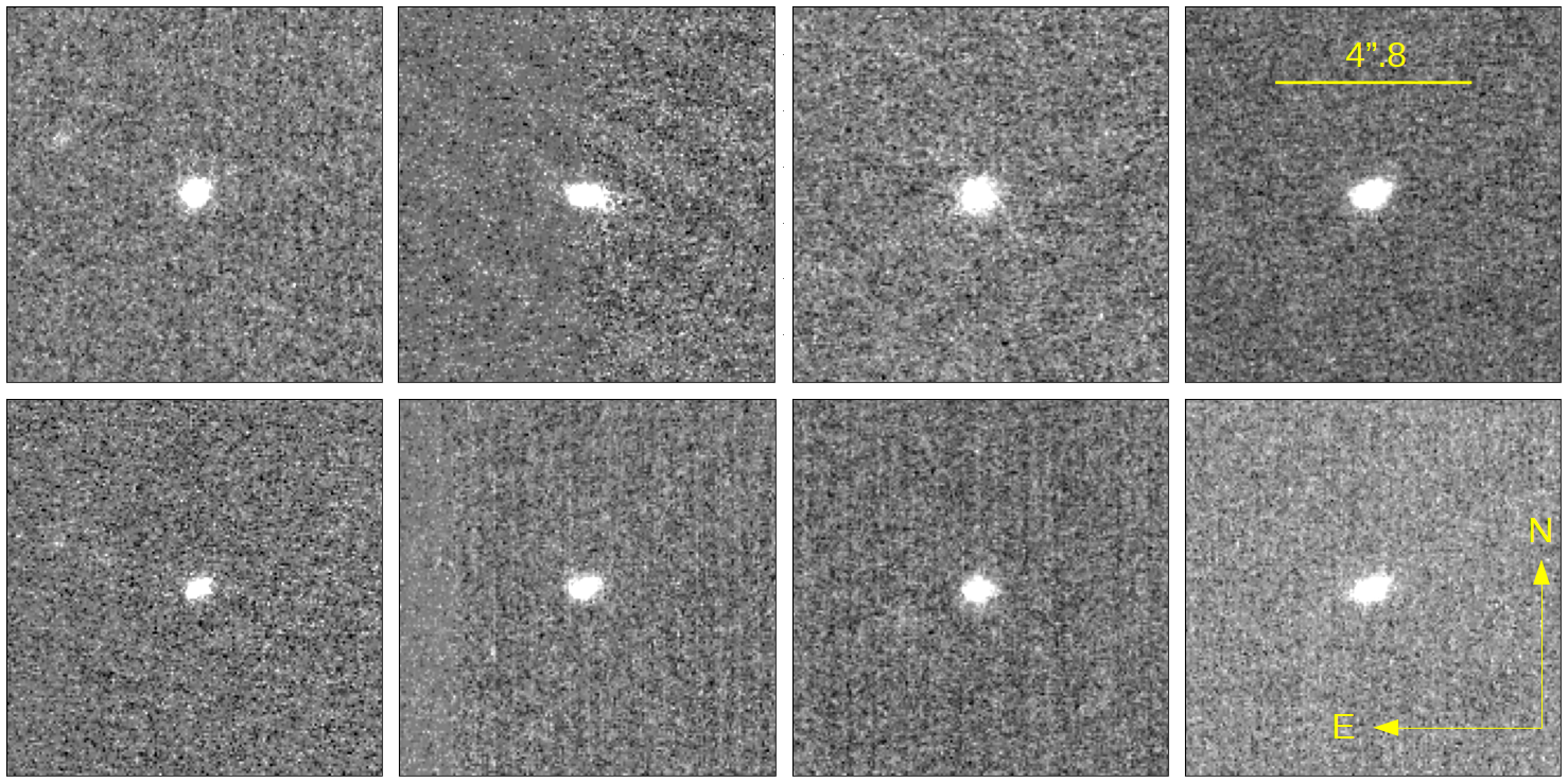
Figure 1: Cutouts of the processed frames around (136199) Eris. Top row: frames in J-band. Bottom row: frames in H-band. Every frame corresponds to a successful observing night (Table 1.), where both bands (J, H) was used to osbserve the target.

3 Photometry results

After performing the aperture photometry we choose to use the 10-pixel-aperture for further analysis because the curve of growth has been flattened enough for that aperture. Differences between the 10-pixel-aperture magnitudes and those of the previous and the next apertures were on the $\sim$0.01 mag level. We used the comparison stars to do standard calibration. First, we converted the $JHK_{s}$ magnitudes of these stars from the 2MASS filter system to the MKO filter system as the latter one was used during the IRTF observations. We applied the transformations from Cutri et al. (2003). We calculated the shift between the instrumental magnitudes and the now MKO magnitudes per filter and per comparison star. We averaged those shifts and took the standard deviation as 1 sigma error for the shift. Then we applied the shift for the instrumental magnitudes of Eris and we calculated the 1 sigma error square as the sum of the square of the instrumental error and the square of the error from the shift.

In order to be able to compare our results with previous J-H values from the literature, we converted the J and H magnitudes of Eris to 2MASS magnitudes from the MKO system using the equations given in Cutri et al. (2003). These previous J-H colours range from $-0.29\pm 0.05$ (Fulchignoni et al., 2008) to $0.287\pm 0.114$ (Snodgrass et al., 2010). The lowest J-H colour values obtained in our measurements are compatible with the lowest J-H values obtained earlier, but even our largest colour index values remain J-H $\leq$ 0.06 mag.

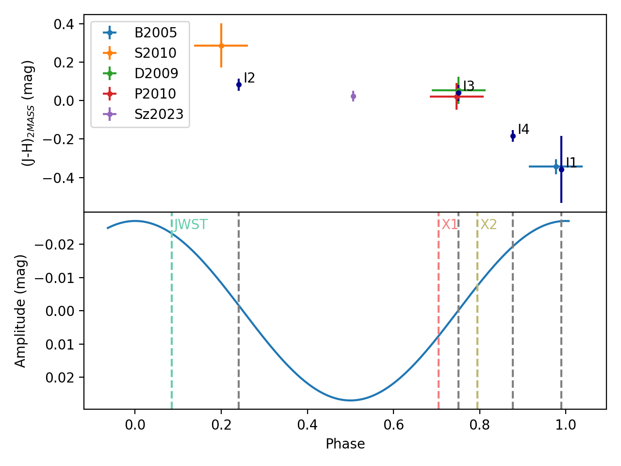
Figure 2: Top: $\mathrm{(J-H)}$  colors of Eris converted to the 2MASS system, as a function of rotational phase (phase zero epoch is 2457357.8929 JD, as obtained from Bernstein et al., 2023). The dark blue markers represent the J-H colors from this work, labeled as I1…I4, from Table 2. The colored markers represent the J-H values from the literature (Table 3). Bottom: An approximate representation of the Eris visible range light curve using a properly phased sinusoidal curve. The phases of IRTF, XShooter (X1 and X2) and JWST/NIRSpec (JWST) measurements are marked by vertical dashed lines.

Table 2: Photometry results of the IRTF near-infrared measurements.

Date	$J_{MKO}$	$H_{MKO}$	$(J-H)_{MKO}$	$(J-H)_{2MASS}$
20230811	17.92 $\pm$ 0.11	18.19 $\pm$ 0.14	-0.27 $\pm$ 0.18	-0.36 $\pm$ 0.18
20230815	17.96 $\pm$ 0.02	17.91 $\pm$ 0.03	0.06 $\pm$ 0.04	0.08 $\pm$ 0.03
20230823	18.01 $\pm$ 0.03	17.96 $\pm$ 0.02	0.04 $\pm$ 0.04	0.04 $\pm$ 0.04
20230825	17.79 $\pm$ 0.02	17.91 $\pm$ 0.03	-0.12 $\pm$ 0.03	-0.18 $\pm$ 0.03

4 Discussion and conclusions

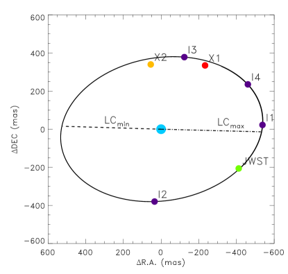
Figure 3: Orbital phasing of the IRTF measurements. We used the ’combined’ orbit solution from Holler et al. (2021) for the epoch 2453979.0 JD: Orbital period P = 15.785899$\pm$0.000050 d; semi-major axis a = 37,273$\pm$64 km; eccentricity e = 0.0062$\pm$0.0010; inclination i = 45.49$\pm$0.15 deg; mean longitude at epoch $\epsilon$ = 125.78$\pm$0.32 deg; longitude of ascending node $\Omega$ = 126.17$\pm$0.26 deg; longitude of periapsis $\varpi$ = 307$\pm$12 deg; The labels I1-I4 at the Dysnomia positions mark the order of the measurements in the IRTF observing sequence (see also Table 1). Dots labeled with ’X1’, ’X2’ and ’JWST’ mark the position and orbital phasing of Dysnomia at the time of first and second X-Shooter measurements, and the JWST/NIRSpec measurement, respectively. Dashed and dash-dotted lines mark the approximate direction of the minimum and maximum of the visible light curve, as determined by Bernstein et al. (2023)

As the orbit of Dysnomia is very accurately known (Holler et al., 2021) it is possible to assign an orbital phase to each IRTF observational epoch. These phases are also representative for the rotational phases of Eris due to the synchronized rotation (Bernstein et al., 2023; Szakáts et al., 2023), and the actual rotational phase can also be calculated using the light curve solution presented in Bernstein et al. (2023).

The actual apparent relative position of Dysnomia with respect to Eris was calculated using the orbital elements of the ’combined’ orbit solution in Holler et al. (2021), as shown in Figs. 2 and 3. In addition, we also calculated the orbital phases for the earlier VLT/XShooter observations (Alvarez-Candal et al., 2011), and the recent James Webb Space Telescope NIRSpec measurement (Grundy et al., 2023). The XShooter and NIRSpec spectra spectra show somewhat different absorption feature depths in the wavelength range covered by the J and H photometric bands, but a direct comparison of these spectra has not been performed in Grundy et al. (2023).

In order to be able to compare our photometric results with those of the previous J-H, measurements (Table 3), we also calculated the approximate phases using data available in the respective papers. Typically only the night of the observation is given, and in some cases the data of two consecutive nights have been merged. While this limits the accuracy of phase determination, an approximate phase even with an error of $\pm$1 d is sufficient due to the long rotation period of Eris. This is reflected in the large phase error bars in Fig. 2. Note that the J-H colour was originally obtained as J-H_s in Snodgrass et al. (2010) and has a large error bar, and shows a J-H value not seen in any other NIR colour measurement of Eris.

While the whole orbital/rotation period of Eris is not covered homogeneously by the J-H measurements, there is a clear correlation between the J-H and the light curve phase (Fig. 2). There are two light curve phases where multiple J-H measurements are available, at $\phi$ $\approx$ 0.75, and $\phi$ $\approx$ 1, with three and two measurements at these phases, respectively. In the respective phases all J-H measurements consistently show the same J-H value. At a phase of $\phi$ $\approx$ 0.2 both our I2 measurement and that by Snodgrass et al. (2010) show a similarly high J-H, however, the latter measurement also has a considerable uncertainty. J-H colors show higher values, J-H $\approx$ 0, around the light curve minimum, roughly between phases $\phi$ $\approx$ 0.2-0.8, and J-H decreases towards the light curve maximum.

Epoch	(J-H)2MASS	(V-R)	Reference
2453396.0	-0.344$\pm$0.039	0.45$\pm$0.02	B2005
2454718.5	0.287$\pm$0.114	0.45$\pm$0.03	S2010
2454362.5	0.054$\pm$0.070	—	D2009
2454441.5	0.022$\pm$0.070	—	P2010
2455439.8	0.024$\pm$0.028	0.358$\pm$0.030	S2023

Table 3: Previously obtained J-H colours of Eris, converted to the 2MASS system. These data are also used for Fig. 2. The columns are: approximate epoch of the observations (see the text for a discussion); J-H colour in the 2MASS system; References: B2005: Brown et al. (2005); S2010: Snodgrass et al. (2010); D2009: Perna et al. (2010); S2023: Szakáts et al. (2023).

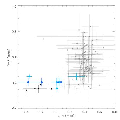
Figure 4: (V-R) vs. (J-H) colours of trans-Neptunian objects, including Eris. Gray dots with error bars represent objects from the MBOSS database, black dots are Haumea-family members. Light blue symbols correspond to the Eris colour measurements from the literature (see Table 3), and dark blue symbols represent the IRTF Eris measurements, assuming an average (V-R) color of 0.406$\pm$0.033.

We compare the J-H colours of Eris with other trans-Neptunian objects in Fig. 4. V-R and J-H colours were taken from the MBOSS2 database (Hainaut et al., 2012). We included Eris measurements from the literature, as well as our new IRTF measurements. We used V-R colours from the literature when it was available (see Table 3). However, this was not the case for all J-H measurements, and the IRTF measurements also lack corresponding V-R colours measured at the same epochs. In these cases we used a mean V-R colour of 0.406$\pm$0.033 mag obtained from the V-R data collected in Szakáts et al. (2023). While the V-R colours of Eris are compatible with the lowest V-R values among trans-Neptunian objects, its J-H colours, observed at any rotational phase, are clearly peculiar, as very few objects show colours J-H $\leq$ 0.1. Most of these objects are members of the Haumea collisional family (see e.g. Snodgrass et al., 2010; Vilenius et al., 2018), characterised by bright and nearly neutrally coloured surfaces (black symbols in Fig. 4). Interestingly, the J-H colour range of Eris, J-H $\approx$ –0.4 – +0.2 is approximately the same that is covered by a number of Haumea family members (1995 SM₅₅, 1999 OY₃, 2005 RS₄₃, 2003 UZ₁₁₇ and Haumea in Fig. 4). However, in the case of Haumea family members the colours are assumed to be due to the presence of water ice which was observed in the spectrum of Haumea (Pinilla-Alonso et al., 2009).

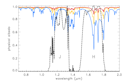
Figure 5: Top panel: Demonstration of the variation of the CH₄ spectrum with particle size in the 0.7–2 $\mu$m wavelength range. Red, orange and blue curves correspond to grain sizes of 100 $\mu$m, 1 mm and 1 cm, respectively. The dash-dotted curve represent the transmission curves of the 2MASS J and H-band filters. Bottom panel: Variation of the (J-H) colour as a function of particle size, assuming pure CH₄ ice, 30 K temperature, and grains of uniform size.

In order to try to explain the variation of the J-H colour of Eris we model the visible – near-infrared spectrum using the version of the Hapke (1993) scattering model presented in Trujillo et al. (2005), applying the same parametrization. As the surface of Eris is strongly dominated by CH₄ ice (Alvarez-Candal et al., 2011; Grundy et al., 2023) we used pure CH₄ in the modeling. Optical constants of CH₄ were obtained from Grundy et al. (2002) and we used three temperatures, 20, 30 and 40 K, and the respective absorption coefficients. We created a set of spectra using particles sizes in the range 10 $\mu$m – 10 cm (Quirico et al., 1999; Trujillo et al., 2005). As demonstrated by our results (Fig. 5), and also in Trujillo et al. (2005) the depth of the absorption bands depends strongly on the particle size, and it is deeper for larger grains. CH₄ has strong absorption bands between 1.6 and 1.8 $\mu$m, strongly affecting the H-band albedo, while the dominant part of the J-band transmittance is between two stronger absorption features and is less affected by the deepening absorption bands with increasing grain size. At the same time, the visible range albedo (in our case at $\sim$0.7 $\mu$m) shows only a very small decrease for larger grain sizes. Using the J and H-band 2MASS transmittance curves (see Skrutskie et al., 2006, and also in Fig. 5) we calculated the expected variation of the J-H color for different grain sizes and temperatures, with respect to the J-H colour at 10 $\mu$m grain size. The results are presented in Fig. 5 and show a substantial decrease in the J-H colour with increasing grain size, reaching a decrease of $\Delta$(J-H) = -0.31 mag at 10 cm grain size. We present here the 30 K curve, but the 20 and 40 K curves are almost identical. If J-H colour variations are to be explained by grain size variations, a $|\Delta$(J-H)$|$ $\approx$ 0.3 mag change would be roughly compatible with our $|\Delta$(J-H)$|$ $\approx$ 0.4 mag variation found in this work, also considering the large errors on the J-H colour derived by Snodgrass et al. (2010), as discussed above. These grain size variations would also leave visible range albedo and brightness nearly unchanged, which is compatible with the very small light curve amplitude of Eris (Szakáts et al., 2023; Bernstein et al., 2023).

A similar range of J-H colour variations can be obtained by assuming large grain sizes all over Eris’ surface and adding different amount of surface constituents which have high visible range albedos but lack absorption bands in the 1-2 $\mu$m wavelength range. The primary candidate would be N₂ which has just recently been detected directly for the first time on the surface of Eris (Grundy et al., 2023) via its broad absorption between 4.0 and 4.3 $\mu$m. The presence of N₂ has long been suspected as for CH₄ molecules dispersed in N₂ ice their vibrational absorption bands appear blue shifted, and the observed spectra suggested that the abundance of N₂ ice could be as high as 90% (Tegler et al., 2010, 2012); a recent spectral modeling by Grundy et al. (2023) obtained a N₂ abundance of 22$\pm$5%.

However, for such large J-H variation that we observe, a very considerable hemispherical difference would be necessary on the surface of Eris, requiring that we see Eris’ surface nearly equator-on. Due to the tidally locked rotation we expect that Eris’ rotational pole is coincident with the pole of Dysnomia’s orbit, and we see the system with a relatively large aspect angle (44°  in 2023). This means that longitudes $|\vartheta|$ $\geq$46°  are continuously visible, and surface regions responsible for the varying J-H colours should be located at $|\vartheta|$ $\leq$46°, relatively close to Eris’ equator. In this configuration the continuously visible polar regions cover $\sim$1/3 of Eris’ observer-facing hemisphere. This limits the possible J-H difference in this current geometry to $\sim$2/3 of the maximum hemispherical difference, and would limit the colour differences due to CH₄ grain size or compositional variations to $\Delta$(J-H) $\approx$ 0.2 mag.

Surface features with large albedo and/or compositional differences are well know to exist on Pluto (see e.g. Cruikshank et al., 2019). As discussed in Hofgartner et al. (2019) at its current heliocentric distance of $\sim$95 au, close to its aphelion, both N₂ and CH₄ are in the local, ballistic atmosphere regime for a significant part of Eris’ surface, and local, collisional atmosphere is expected only at the warmest parts, near the subsolar latitudes. Grundy et al. (2023) explained the observed D/H and ¹³CO/¹²CO isotopic rations by a possible geologically recent outgassing from the interiors or with processes that cycle the surface methane inventory to keep the uppermost surfaces refreshed – these processes may not occur homogeneously on the entire surface. While the current spectroscopic observations of Eris does not show major compositional differences at the different rotational phases, the observed variations in the J-H colour, presented in this paper, clearly indicates that there should be variegations in composition, grain size, or other surface properties that affect the near-infrared reflectance significantly. Additional visible/near-infrared spectra obtained at specific rotational phases could help to determine what effects can be responsible for the J-H colour variations. Presently the instrument most suitable to perform these kind of observations is the NIRSpec spectrometer of the James Webb Space Telescope as this is the only instrument that could directly confirm the presence N₂ on the surface of Eris.

References

- Alvarez-Candal et al. (2020) Alvarez-Candal, A., Souza-Feliciano, A. C., Martins-Filho, W., Pinilla-Alonso, N., & Ortiz, J. L. 2020, MNRAS, 497, 5473, doi: 10.1093/mnras/staa2329
- Alvarez-Candal et al. (2011) Alvarez-Candal, A., Pinilla-Alonso, N., Licandro, J., et al. 2011, A&A, 532, A130, doi: 10.1051/0004-6361/201117069
- Astropy Collaboration et al. (2013) Astropy Collaboration, Robitaille, T. P., Tollerud, E. J., et al. 2013, A&A, 558, A33, doi: 10.1051/0004-6361/201322068
- Astropy Collaboration et al. (2018) Astropy Collaboration, Price-Whelan, A. M., Sipőcz, B. M., et al. 2018, AJ, 156, 123, doi: 10.3847/1538-3881/aabc4f
- Astropy Collaboration et al. (2022) Astropy Collaboration, Price-Whelan, A. M., Lim, P. L., et al. 2022, apj, 935, 167, doi: 10.3847/1538-4357/ac7c74
- Bernstein et al. (2023) Bernstein, G. M., Holler, B. J., Navarro-Escamilla, R., et al. 2023, arXiv e-prints, arXiv:2303.13445, doi: 10.48550/arXiv.2303.13445
- Bradley et al. (2023) Bradley, L., Sipőcz, B., Robitaille, T., et al. 2023, astropy/photutils: 1.8.0, 1.8.0, Zenodo, doi: 10.5281/zenodo.7946442
- Brown et al. (2005) Brown, M. E., Trujillo, C. A., & Rabinowitz, D. L. 2005, ApJ, 635, L97, doi: 10.1086/499336
- Cruikshank et al. (2019) Cruikshank, D. P., Grundy, W. M., Jennings, D. E., et al. 2019, in Remote Compositional Analysis: Techniques for Understanding Spectroscopy, Mineralogy, and Geochemistry of Planetary Surfaces, ed. J. L. Bishop, I. Bell, James F., & J. E. Moersch (Cambridge University Press), 442–452, doi: 10.1017/9781316888872.024
- Cutri et al. (2003) Cutri, R., Skrutskie, M., Van Dyk, S., et al. 2003, Explanatory supplement to the 2MASS all Sky Data release and Extended Mission Products. https://www.ipac.caltech.edu/2mass/releases/allsky/doc/explsup.html
- DeMeo et al. (2009) DeMeo, F. E., Binzel, R. P., Slivan, S. M., & Bus, S. J. 2009, Icarus, 202, 160, doi: 10.1016/j.icarus.2009.02.005
- Fernández-Valenzuela et al. (2021) Fernández-Valenzuela, E., Pinilla-Alonso, N., Stansberry, J., et al. 2021, \psj, 2, 10, doi: 10.3847/PSJ/abc34e
- Fulchignoni et al. (2008) Fulchignoni, M., Belskaya, I., Barucci, M. A., de Sanctis, M. C., & Doressoundiram, A. 2008, in The Solar System Beyond Neptune, ed. M. A. Barucci, H. Boehnhardt, D. P. Cruikshank, A. Morbidelli, & R. Dotson (University of Arizona Press), 181
- Grundy et al. (2002) Grundy, W. M., Schmitt, B., & Quirico, E. 2002, Icarus, 155, 486, doi: 10.1006/icar.2001.6726
- Grundy et al. (2023) Grundy, W. M., Wong, I., Glein, C. R., et al. 2023, arXiv e-prints, arXiv:2309.05085, doi: 10.48550/arXiv.2309.05085
- Hainaut et al. (2012) Hainaut, O. R., Boehnhardt, H., & Protopapa, S. 2012, A&A, 546, A115, doi: 10.1051/0004-6361/201219566
- Hapke (1993) Hapke, B. 1993, Theory of reflectance and emittance spectroscopy (Cambridge University Press)
- Hofgartner et al. (2019) Hofgartner, J. D., Buratti, B. J., Hayne, P. O., & Young, L. A. 2019, Icarus, 334, 52, doi: 10.1016/j.icarus.2018.10.028
- Holler et al. (2021) Holler, B., Bannister, M. T., Singer, K. N., et al. 2021, in Bulletin of the American Astronomical Society, Vol. 53, 228, doi: 10.3847/25c2cfeb.5950ca1c
- Kecskeméthy et al. (2023) Kecskeméthy, V., Kiss, C., Szakáts, R., et al. 2023, ApJS, 264, 18, doi: 10.3847/1538-4365/ac9c67
- Lacerda (2009) Lacerda, P. 2009, AJ, 137, 3404, doi: 10.1088/0004-6256/137/2/3404
- Lacerda et al. (2008) Lacerda, P., Jewitt, D., & Peixinho, N. 2008, AJ, 135, 1749, doi: 10.1088/0004-6256/135/5/1749
- Nimmo et al. (2017) Nimmo, F., Umurhan, O., Lisse, C. M., et al. 2017, Icarus, 287, 12, doi: 10.1016/j.icarus.2016.06.027
- Perna et al. (2010) Perna, D., Barucci, M. A., Fornasier, S., et al. 2010, A&A, 510, A53, doi: 10.1051/0004-6361/200913654
- Pinilla-Alonso et al. (2009) Pinilla-Alonso, N., Brunetto, R., Licandro, J., et al. 2009, A&A, 496, 547, doi: 10.1051/0004-6361/200809733
- Quirico et al. (1999) Quirico, E., Douté, S., Schmitt, B., et al. 1999, Icarus, 139, 159, doi: 10.1006/icar.1999.6111
- Rayner et al. (2003) Rayner, J. T., Toomey, D. W., Onaka, P. M., et al. 2003, PASP, 115, 362, doi: 10.1086/367745
- Skrutskie et al. (2006) Skrutskie, M. F., Cutri, R. M., Stiening, R., et al. 2006, AJ, 131, 1163, doi: 10.1086/498708
- Snodgrass et al. (2010) Snodgrass, C., Carry, B., Dumas, C., & Hainaut, O. 2010, A&A, 511, A72, doi: 10.1051/0004-6361/200913031
- Szakáts et al. (2020) Szakáts, R., Müller, T., Alí-Lagoa, V., et al. 2020, A&A, 635, A54, doi: 10.1051/0004-6361/201936142
- Szakáts et al. (2023) Szakáts, R., Kiss, C., Ortiz, J. L., et al. 2023, A&A, 669, L3, doi: 10.1051/0004-6361/202245234
- Tegler et al. (2012) Tegler, S. C., Grundy, W. M., Olkin, C. B., et al. 2012, ApJ, 751, 76, doi: 10.1088/0004-637X/751/1/76
- Tegler et al. (2010) Tegler, S. C., Cornelison, D. M., Grundy, W. M., et al. 2010, ApJ, 725, 1296, doi: 10.1088/0004-637X/725/1/1296
- Trujillo et al. (2005) Trujillo, C. A., Brown, M. E., Rabinowitz, D. L., & Geballe, T. R. 2005, ApJ, 627, 1057, doi: 10.1086/430337
- Vernazza et al. (2021) Vernazza, P., Ferrais, M., Jorda, L., et al. 2021, A&A, 654, A56, doi: 10.1051/0004-6361/202141781
- Vilenius et al. (2018) Vilenius, E., Stansberry, J., Müller, T., et al. 2018, A&A, 618, A136, doi: 10.1051/0004-6361/201732564