Goal-Oriented Wireless Communication
Resource Allocation for Cyber-Physical Systems

Abstract

The proliferation of novel industrial applications at the wireless edge, such as smart grids and vehicle networks, demands the advancement of cyber-physical systems (CPSs). The performance of CPSs is closely linked to the last-mile wireless communication networks, which often become bottlenecks due to their inherent limited resources. Current CPS operations often treat wireless communication networks as unpredictable and uncontrollable variables, ignoring the potential adaptability of wireless networks, which results in inefficient and overly conservative CPS operations. Meanwhile, current wireless communications often focus more on throughput and other transmission-related metrics instead of CPS goals. In this study, we introduce the framework of goal-oriented wireless communication resource allocations, accounting for the semantics and significance of data for CPS operation goals. This guarantees optimal CPS performance from a cybernetic standpoint. We formulate a bandwidth allocation problem aimed at maximizing the information utility gain of transmitted data brought to CPS operation goals. Since the goal-oriented bandwidth allocation problem is a large-scale combinational problem, we propose a divide-and-conquer and greedy solution algorithm. The information utility gain is first approximately decomposed into marginal utility information gains and computed in a parallel manner. Subsequently, the bandwidth allocation problem is reformulated as a knapsack problem, which can be further solved greedily with a guaranteed sub-optimality gap. We further demonstrate how our proposed goal-oriented bandwidth allocation algorithm can be applied in four potential CPS applications, including data-driven decision-making, edge learning, federated learning, and distributed optimization. Through simulations, we confirm the effectiveness of our proposed goal-oriented bandwidth allocation framework in meeting CPS goals.

I Introduction

The wireless edge is witnessing a proliferation of new industrial applications that span areas such as smart grids, vehicle networks, and the Internet of Things. These applications predominantly involve data-centric tasks, including data-driven decision-making, prediction, and control [1]. As a result, they are transitioning into cyber-physical systems (CPSs), whose performance is influenced by both their physical components and wireless communication networks [2].

The surge in data traffic and the extensive access demands in CPSs present significant challenges for wireless communications [3]. To address that, the communication community is innovating strategies to optimize the management of wireless communication networks. A key advancement is semantic communication [4], which considers data importance and semantics, not just symbols in communications [5]. In contrast to the conventional Shannon paradigm, semantic communications only transmit necessary information relevant to specific tasks. The transmission of irrelevant information is omitted [6].

Meanwhile, stakeholders in CPS-related domains gradually recognize the crucial role of wireless communication networks [7]. Delays, reliability, and other factors can affect the CPS operation goals [8]. For example, increased delays and reduced reliability can lead to suboptimal decisions and increase system costs. However, these industries often view wireless communications as unpredictable, unmanageable, and potentially adverse factors in CPSs [9]. This perspective may be rooted in conventional communication networks, which prioritize data delivery based on transmission-related objectives, without considering their impact on physical systems. However, in reality, the communication network can be tailored to cater to the customized needs of CPS task goals [10].

An evident research gap remains: how to measure the contribution of data semantics to CPS operation goals, and how to subsequently manage radio resource allocations in assisting CPSs in achieving their goals?

I-A Related Works

I-A1 CPS Operation Considering Effects of Communication

Using smart grids as a typical example of the CPS, researchers examined the effects of communication delays and losses on system stability and operations. Ref.[11] investigated the effects of communication delays on micro-grid small-signal stability, while Ref.[12] explored the effects of communication reliability on demand response. Further studies investigated the influence of communications on distributed algorithms, including distributed economic dispatch [13] and distributed frequency regulation services [14].

Traditionally, these works perceived communication as unpredictable, difficult to manage, and possibly detrimental. To mitigate such adverse effects, decentralized [15], quantized [16], and event-triggered algorithms [17] were designed. These approaches aimed to curtail data traffic, thereby reducing the potential negative consequences of communication networks [18]. However, as the saying goes, ’there is no free lunch.’ These communication-efficient algorithms, while reducing data traffic, introduced increased complexity. Crucially, communication networks are not always unmanageable or invariably harmful. Our work aims to challenge the stereotype that communication networks in CPSs are unmanageable.

I-A2 Semantic, Task-oriented, and Goal-oriented Communications

The field of semantic communication has earned significant interest from both academia and industry. Refs.[19, 20] offered a comprehensive review of semantic communications. Notably, the semantics of the same piece of data can vary based on its intended task [21]. Consequently, some researchers have refined semantic communications to be task-oriented and goal-oriented, emphasizing the extraction and transmission of only task-relevant information [22]. Goal-oriented communication is expected to be integrated into future 6G communication standards [23].

Many researchers have devoted efforts to designing appropriate encoders and decoders for goal-oriented communications, moving beyond Shannon’s paradigm [24, 25]. It was recognized that extracting semantics based solely on human experiences is challenging [26]. Typically, deep learning techniques have been employed to extract the underlying semantics of data [27]. While machine learning methods are prevalent, some studies have attempted to integrate information theory to enhance the interpretability of results [28]. Our work focuses on radio resource management rather than codebook design.

I-A3 Efficient Communications for Learning

The rise of learning-related tasks has sparked extensive research about communication-efficient learning [29]. Some studies focused on data compression and quantization to reduce data traffic, similar to techniques used in the communication-efficient distributed design [30]. Interestingly, another subset of research developed the importance-aware approach to identify valuable data in learning tasks and reduce unnecessary data communications. This approach closely aligns with the spirit of semantic and goal-oriented communications. In the context of data sample transmissions, Ref.[31] developed a communication rule based on data importance to train a model. Many studies investigated learning problems in a distributed setting, mostly referred to federated learning [32]. Refs.[33, 34, 35] employed various criteria to identify the importance of gradient updates, subsequently scheduling participation and consequently reducing the overall training time. In fact, our analysis demonstrates that learning can be viewed as a specific CPS task aimed at minimizing training loss and maximizing inference accuracy in the shortest possible time. Our framework extends to a broader range of CPS applications and is not confined solely to learning.

I-B Contributions and Organizations

In this study, we introduce the unified framework for goal-oriented radio resource allocation in CPSs. Our objective is to bridge the gap between the communication community and other CPS domains. For communications, we analytically evaluate the contributions of transmitted data and develop a goal-oriented bandwidth allocation approach that smoothly integrates with current systems. For other CPS domains, we aim to show that the communication network can be tailored to improve CPS performance and better fulfill its goals. Our major contributions include:

• Introduce a unified framework for goal-oriented radio resource management in CPSs. We formulate a wireless Resource Block (RB) Allocation (RBA) problem in orthogonal frequency division multiple access (OFDMA) based wireless communication networks. The RBA problem maximizes the information utility gain, instead of throughput-related objectives, to better ensure the realization of the CPS goals under constraints of limited radio resources.

• Propose a divide-and-conquer and greedy solution approach to the goal-oriented RBA problem, taking into account its combinatorial complexity and other practical considerations. The information utility gain is divided into the sum of marginal information utility gains, enhancing problem parallelism. The goal-oriented RBA problem is then reformulated as a knapsack problem with limited RB capacity, solved via a greedy method with a sub-optimality gap guarantee and reduced complexity.

• Develop application-specific designs of the goal-oriented RBA for four representative CPS applications. The specific approach to calculating the information utility gain for different applications is further detailed. The applications either require massive connections or large-volume data transmissions, covering common CPS applications including decision-making, learning, and optimization. We use smart grids and vehicle networks as examples of CPS systems to explain specific applications.

• Conduct a simulation to verify the effectiveness of the goal-oriented RBA in CPSs. The performance of the proposed RBA method is compared against throughput maximization and pure data utility RBA policies, in terms of both throughput and CPS goal values. The results highlight the advantages of the proposed goal-oriented RBA framework in guaranteeing CPS goals under limited radio resource constraints.

The remainder of this paper is structured as follows: Section II introduces the system model. Section III outlines the solution challenges, develops the solution method, and addresses practical concerns. Section IV details the computation of information utility gains for four applications: data-driven decision-making, edge learning, federated learning, and distributed optimization. Section V presents case studies, followed by conclusions in Section VI.

Notations: The following conventions are used in this paper: Scalars are represented in normal font. Vectors and matrices are represented in bold font. $\mathbf{0}$ represents a zero matrix/vector, $\mathbf{I}$ indicates the identity matrix. $\bigcup_{i=1}^{n}S_{i}$ indicates arbitrary unions of set $S_{1}\cup S_{2}\cup S_{3}\cup\cdots\cup S_{n}$. $|\boldsymbol{x}|$ denotes the cardinality of the set $\boldsymbol{x}$. $\mathbb{P}$ represents probability distributions, and $\mathbb{E}$ denotes mathematical expectations. $\|\boldsymbol{x}\|_{2}$ and $\|\mathbf{x}\|_{F}$ indicate vector $\boldsymbol{x}$’s 2 norm and matrix $\mathbf{x}$’s Frobenius norm, respectively. $\nabla$ and $\nabla^{2}$ indicate the gradient and the second-order partial derivatives, respectively. $\left<\boldsymbol{x},\boldsymbol{y}\right>=\boldsymbol{x}^{\top}\boldsymbol{y}$ denotes the inner product. $\lceil x\rceil$ denotes the round up functions of $x$.

II System Model

II-A Cyber-physical System Architecture

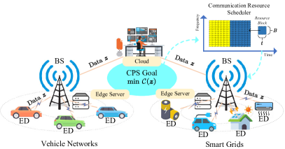
Figure 1: The architecture of the cyber-physical system. The system’s ultimate objective is to minimize $\mathcal{C}\left(\boldsymbol{z}\right)$, which is a function of available data $\boldsymbol{z}$. Goal-oriented RBA aims to allocate limited communication resources to EDs that are more relevant and important to minimizing the cost function $\mathcal{C}\left(\boldsymbol{z}\right)$.

The architecture of the CPS is illustrated in Fig.1. The physical subsystem comprises various end devices (EDs), labeled as $j=1,...,J$. In the context of smart grids, EDs might include solar panels, home appliances like air conditioners, and energy storage. For vehicle networks, EDs mainly represent on-road electric vehicles. The cyber subsystem mostly involves the communication system. In this study, we mainly focus on the uplink communication network.

Within this framework, a CPS operator carries out specific tasks. Usually, CPS operators will process these tasks on nearby (edge) servers or larger cloud servers. The process is as follows: the operator first collects fresh data from the EDs, usually over cellular networks facilitated by base stations (BSs). After receiving this data, operators analyze it at the edge server or the cloud, determine optimal strategies, and if needed, send commands back to the EDs. The operator’s ultimate objective is to minimize system cost $\mathcal{C}\left(\boldsymbol{z}\right)$, contingent on the data $\boldsymbol{z}$. Different applications may present different forms of the objective $\mathcal{C}(\cdot)$ and will be further illustrated in the subsequent sections. For instance, in smart grids, a load aggregator (the operator) might monitor the electricity consumption of EDs and perform demand response; in vehicle networks, the traffic management entities (the operator) aim to optimize traffic flow and prevent car accidents. The concrete expressions of $\mathcal{C}\left(\boldsymbol{z}\right)$ will be further explained in section IV.

II-B Wireless Communication Model

We assume that orthogonal frequency division multiple access (OFDMA) is utilized for uplink data transmissions. Following LTE (Long-Term Evolution) and 5G cellular communication standards, we use resource block (RB) as the basic unit of resources allocated to EDs in both the frequency and time domains, as shown in Fig.1. For a given RB, labeled as $i$, the data it can deliver (in bits), denoted as $r_{i,j}$, when assigned to ED $j$ is determined by:

$$r_{i,j}=tB\log_{2}\left(1+\frac{g_{j}p_{j}}{\sigma^{2}}\right)$$ (1)

where $t$ is the time duration of RB $i$. $B$ defines the bandwidth of RB $i$. $g_{j}$ is the channel gain between the cellular BS and ED $j$. $\sigma^{2}$ is the channel noise. $p_{j}$ is the transmitting power of ED $j$.

During a time period of $T$ with a total of $I$ RBs, the cumulative data bits that an ED $j$ can transmit are given by:

$$r_{j}=\sum\nolimits_{i=1}^{I}{a_{i,j}tB\log_{2}\left(1+\frac{g_{j}p_{j}}{\sigma^{2}}\right)}$$ (2)

where $a_{i,j}$ denotes channel allocations, with $a_{i,j}=1$ indicating RB $i$ is allocated to $j$. Otherwise, it equals $0$.

The focus of this paper is the uplink transmission. Historically, the uplink channel (from EDs to the BSs) often received a smaller share of the communication bandwidth. Consequently, the uplink channel often serves as the bottleneck of the whole network. In most cases, downlink transmissions in CPS applications are broadcast and do not lead to communication congestion.

II-C Goal-oriented RBA Problem

We focus on the communication system’s channel allocation among various EDs, with the aim of maximizing the total information utility gain, while adhering to communication resource budget constraints. The whole problem can be formulated as (P1) below:

$$\max_{a_{i,j},s_{j}}\,\, \mathcal{C}\left(\boldsymbol{z}_{\mathrm{old}}\right)-\mathcal{C}\left(\boldsymbol{z}_{\mathrm{new}}\right)$$ (3)

$$\mathrm{s}.\mathrm{t}.\,\, \sum\nolimits_{i=1}^{I}{a_{i,j}tB\log_{2}\left(1+\frac{g_{j}p_{j}}{\sigma^{2}}\right)}\geqslant s_{j}r_{\min,j}$$ (4)

$$\left(\mathbf{P1}\right)~{}~{}~{}~{}~{} \sum\nolimits_{j=1}^{J}{a_{i,j}=1,}~{}~{}\forall i$$ (5)

$$a_{i,j}\in\left\{0,1\right\},s_{j}\in\left\{0,1\right\},~{}~{}\forall i,j$$ (6)

$$\boldsymbol{z}_{\mathrm{new}}=\boldsymbol{z}_{\mathrm{old}}\cup\left\{\bigcup{s_{j}\boldsymbol{z}_{j}^{+}}\right\}$$ (7)

where the decision variables are channel allocations $a_{i,j}$, and ED $j$ transmission permission $s_{j}$ (determining whether ED $j$’s data transmission is allowed). $a_{i,j}$ and $s_{j}$ are both binary variables. $a_{i,j}=1$ indicates RB $i$ is allocated to ED $j$. $s_{j}=1$ implies ED $j$ is allocated sufficient communication resources to facilitate data transmission. The existing dataset before communication is represented by $\boldsymbol{z}_{\mathrm{old}}$, while $\boldsymbol{z}_{j}^{+}$ denotes the new data generated by ED $j$, which is not yet known to the CPS operator. $\boldsymbol{z}_{\mathrm{new}}$ denotes all the data that the CPS operator has acquired after the communication process.

In problem (P1), the objective is to maximize the total information utility gain: the difference in the anticipated system costs $\mathcal{C}\left(\boldsymbol{z}_{\mathrm{new}}\right)$ after new data are transmitted and the cost $\mathcal{C}\left(\boldsymbol{z}_{\mathrm{old}}\right)$ before any data transmission occurs. A particular instance of the problem (P1) is when the cost function equals the dataset’s cardinality, $\mathcal{C}\left(\boldsymbol{z}\right)=-|\boldsymbol{z}|$. This implies that acquiring more data consistently reduces costs without accounting for data semantics, which is the conventional practice. However, in this context, we can select $\mathcal{C}\left(\boldsymbol{z}\right)$ aligned with the CPS operator’s goal. The communication paradigm shifts to maximizing the benefit of data to system goals.

Constraint Eq.(4) imposes a restriction to ensure the minimal requirements for reliable data communications: ED $j$’s data can be transmitted ($s_{j}=1$) if, and only if, the cumulatively allocated channels can assure the minimum reliable data rate $r_{\min,j}$ is met. Constraint Eq.(5) ensures that a single resource block can only be allocated to one ED. Eq.(7) specifies that the latest dataset $\boldsymbol{z}_{\mathrm{new}}$ that the operators possess is the union set of the old dataset $\boldsymbol{z}_{\mathrm{old}}$ and the freshly transmitted data ${s_{j}\boldsymbol{z}_{j}^{+}}$.

III Solution Methods

TABLE I: Symbol Description

Symbol	Description
Sets
$i=1,...,I$	RB Index
$j=1,...,J$	ED Index
$k=1,...,K$	Iteration Round Index
$d=1,...,D_{j}$	Data Sample Index
Variables
$a_{i,j}$	Channel Allocations
$s_{j}$	Transmission Permissions
$\boldsymbol{\pi}$	Decisions and Actions (Data-driven Decision Problems)
$\boldsymbol{\theta},\boldsymbol{\theta}^{+}$	Model Weights (Edge & Federated Learning)
$\cdot\cdot\cdot$	$\cdot\cdot\cdot$

Symbol	Description
$\boldsymbol{g},\tilde{\boldsymbol{g}}$	Model Gradients (Federated Learning)
$\boldsymbol{\theta}_{0},\boldsymbol{\theta}_{j}$	Decision Variables (Distributed Optimization)
$\boldsymbol{\lambda}$	Dual Variables (Distributed Optimization)
Parameters
$t$	Time Duration of RBs
$B$	Bandwidth of RBs
$g_{j}$	Channel Gains
$p_{j}$	Transmitting Power
$\sigma$	Channel Noise
$\cdot\cdot\cdot$	$\cdot\cdot\cdot$

Symbol	Description
$\boldsymbol{z}_{\mathrm{old}},\boldsymbol{z}^{+},\boldsymbol{z}_{\mathrm{new}}$	Old Data, Freshly Transmitted Data, Total Data After Transmissions
$\boldsymbol{\xi}$	Boundary Parameters (Data-driven Decision)
$\mathsf{z}_{j}$	Raw Data Samples
Functions
$\mathcal{C}(\cdot)$	CPS Goal
$h(\cdot)$	Decision Cost (Data-driven Decision Problems)
$L(\cdot),\ell(\cdot)$	Loss Function (Edge & Federated Learning)
$\mathcal{L}(\cdot)$	Augmented Lagrangian Function (Distributed Optimization)

III-A Solution Challenges

The goal-oriented RBA problem (P1) is a large-scale combination problem. Direct approaches to solving P1 are hindered by the following computational and practical challenges:

• Exponential Computation Complexity: The binary nature of the variable $s_{j}$ implies that $\boldsymbol{z}_{\mathrm{new}}=\boldsymbol{z}_{\mathrm{old}}\cup\left\{\bigcup{s_{j}\boldsymbol{z}_{j}^{+}}\right\}$ possesses an exponential array of potential combinatorial values. This necessitates the computation of all feasible permutations of $\mathcal{C}\left(\boldsymbol{z}_{\mathrm{new}}\right)$, corresponding to all possible combinations of $s_{j}$. Consequently, this leads to an exponential computational complexity quantified as $2^{\sum\nolimits_{j}{|\boldsymbol{z}_{j}^{+}|}}$, where $|\boldsymbol{z}_{j}^{+}|$ signifies the cardinality of ED $j$’s dataset.

• Non-Causal Paradox of Future Data: The objective function of the problem (P1) can be theoretically computed when $\boldsymbol{z}_{\mathrm{new}}$ is known. In practical scenarios, this latest dataset isn’t available until communication takes place. Hence, performing RBA based on future data is non-causal and not feasible.

• Complexity and Optimality Gap Trade-off: The goal-oriented RBA will incur extra overhead and delay for CPSs. If the additional computational overhead is significantly high, it can introduce latency and potentially offset the benefits obtained through the goal-oriented RBA. The practical solution should balance the complexity and the gap to the ideal optimal solution.

In the following three subsections, we will systematically address these aforementioned challenges.

III-B Divide-and-Conquer Approach

We begin by simplifying the computation of the information utility gain. We assume that the information utility gain approximately satisfies the submodular property, shown below:

Assumption 1.

The negative CPS goal $-\mathcal{C}(\boldsymbol{z})$ is a submodular function or can be closely approximated by a submodular function. This is defined in the following manner: For every dataset $\boldsymbol{z}$ and $\boldsymbol{z}_{1},\boldsymbol{z}_{2}\notin\boldsymbol{z}$ such that $\boldsymbol{z}_{1}\neq\boldsymbol{z}_{2}$, we have that $-\mathcal{C}\left(\boldsymbol{z}\cup\left\{\boldsymbol{z}_{1}\right\}\right)-\mathcal{C}\left(\boldsymbol{z}\cup\left\{\boldsymbol{z}_{2}\right\}\right)\geq-\mathcal{C}\left(\boldsymbol{z}\cup\left\{\boldsymbol{z}_{1},\boldsymbol{z}_{2}\right\}\right)-\mathcal{C}\left(\boldsymbol{z}\right)$.

Submodular functions are widely used in game theory and machine learning, meaning that obtaining more information is beneficial, but the marginal return diminishes as the dataset grows. With the submodular property, the total information utility gain can be bounded as follows:

Proposition 1.

When the negative CPS goal satisfies the submodular property, the total information gain can be bounded by the sum of individual information utility gain $\Delta_{j}$, shown as below:

$$\mathcal{C}\left(\boldsymbol{z}_{\mathrm{old}}\right)-\mathcal{C}\left(\boldsymbol{z}_{\mathrm{old}}\cup\left\{\bigcup{s_{j}\boldsymbol{z}_{j}^{+}}\right\}\right)$$ (8)

$$\leqslant \sum\nolimits_{j}{\mathcal{C}\left(\boldsymbol{z}_{\mathrm{old}}\right)-\mathcal{C}\left(\boldsymbol{z}_{\mathrm{old}}\cup\left\{s_{j}\boldsymbol{z}_{j}^{+}\right\}\right)}$$

$$\left(\mathbf{P2}\right)~{}~{}= \sum\nolimits_{j}{s_{j}\underset{\Delta_{j}}{\underbrace{\left(\mathcal{C}\left(\boldsymbol{z}_{\mathrm{old}}\right)-\mathcal{C}\left(\boldsymbol{z}_{\mathrm{old}}\cup\left\{\boldsymbol{z}_{j}^{+}\right\}\right)\right)}}}$$

Instead of maximizing the total information utility gain, we maximize its upper bound and replace the objective function as (P2). This approach allows for independent computation of the information utility gain $\Delta_{j}$ for each device. Consequently, this allows for parallel computing, reducing the exponential complexity to a linear complexity characterized by $\sum\nolimits_{j}{|\boldsymbol{z}_{j}^{+}|}$.

III-C Causality Problem

There are two methods to solve the non-causal challenges.

III-C1 Large Payload Size Case

Sometimes, the data $\boldsymbol{z}^{+}$ to be transmitted is very large. For instance, images and model gradients often have large sizes. In contrast, the marginal information utility is just a single numerical value. To manage this, EDs can first send the value of the marginal information utility gain to the server. The server operator then decides which EDs should send their full data. Using this method, the operator can tackle (P2) based on the given utility values.

III-C2 Small Payload Size Case

When the data payload is minimal, sending extra data can lead to added congestion in the wireless communication network. Under such circumstances, a practical solution involves sampling fresh data, $\boldsymbol{z}_{+}$, using historical data, $\boldsymbol{z}_{\mathrm{old}}$, under the assumption that $\boldsymbol{z}_{+}$ has the same probabilistic distribution as $\boldsymbol{z}_{\mathrm{old}}$. This method leads us to a new optimization problem (P3) where the information utility gain is switched to the expected marginal information utility gain:

$$\left(\mathbf{P3}\right)~{}~{}~{}\max_{a_{i,j},s_{j}}\,\,\sum\nolimits_{j}{\mathbb{E}_{\boldsymbol{z}_{\mathrm{old}}}\left[s_{j}\Delta_{j}\right]}$$ (9)

where $\mathbb{E}_{\boldsymbol{z}_{\mathrm{old}}}[\cdot]$ represents the expected value based on old data, providing a prediction of potential information gain in upcoming data. This method tends to perform well when there is a strong temporal correlation between consecutive transmitted data.

III-D Greedy Solutions and Sub-optimality Guarantee

Upon calculating the marginal information utility gain, problems (P2-P3) can be converted to the knapsack problem, a well-known combinatorial problem. The communication channel can be converted to a knapsack with a limited capacity of $J$ units. ED $j$ will utilize $w_{j}$ channel units if selected for the ‘knapsack’, where $w_{j}$ represents the minimum channel units required to meet the constraint in Eq.(4):

$$w_{j}=\lceil\frac{r_{\min,j}}{Bt\log_{2}\left(1+\frac{g_{j}p_{j}}{\sigma^{2}}\right)}\rceil$$ (10)

The benefit derived from ED $j$ corresponds to its marginal information utility gain, which is $\Delta_{j}\geqslant 0$. In summary, (P2-P3) can be transformed into the following problem (P4):

$$\left(\mathbf{P}\mathbf{4}\right)~{}~{}~{}~{}\max_{s_{j}}{}{} \sum\nolimits_{j}{\Delta_{j}s_{j}}$$ (11)

$$\mathrm{s}.\mathrm{t}.{}{} \sum\nolimits_{j}{w_{j}s_{j}\leqslant J},~{}s_{j}\in\left\{0,1\right\}$$

The knapsack problem is widely recognized as NP-hard, resulting in significant computational overhead. To address this, we employ a greedy algorithm, depicted in Algorithm 1. Despite its greedy nature, the algorithm’s suboptimal loss can be bounded in relation to the theoretical optimum of (P4):

Proposition 2.

If $w_{j}\leqslant\eta J$ for every ED $j$, with $\eta\in\left(0,\frac{1}{2}\right]$, then the solution computed in Algorithm 1 guarantees at least $1-\eta$ of the optimal solution of (P2)-(P3).

The proof is provided in Section 2.2 of Ref.[36]. The assumption $w_{j}\leqslant\eta J$ indicates that a single ED will not consume too many RBs. The most complex part of the greedy solution method is to sort the EDs with respect to $\frac{\Delta_{j}}{w_{j}}$. Utilizing an efficient sorting algorithm results in a time complexity of $O(J\mathrm{log}J)$, allowing for swift execution on edge servers.

In summary, with all these techniques, the complete goal-oriented RBA process is shown in Algorithm 2 and 3, for large-size payload and small-size payload, respectively. The entire process is designed to operate in parallel. Importantly, the algorithm is tailored to seamlessly integrate with today’s cellular communication protocols. Currently, the channel allocations are based on the channel qualities $g_{j}$ detected using pilot frequencies.

Input: $w_{j}$,$\Delta_{j}$

1 Step 1: Sort and re-index the EDs so that:

$$\frac{\Delta_{1}}{w_{1}}\geq\frac{\Delta_{2}}{w_{2}}\geq\cdots\geq\frac{\Delta_{J}}{w_{J}}.$$

2 Step 2: Pick EDs in this order until the channel budget is used up, and then halt.

Result: $j\in\{j|s_{j}=1\}$

Algorithm 1 Hybrid Allocation Rule

1 Parallel Thread 1: Using pilot frequencies to identify channel gain $g_{j}$, and compute $w_{j}$.

2 Parallel Thread 2:

3 Information Utility Update: All EDs upload $\Delta_{j}$.

4 Channel Allocations: The operator employs Algorithm 2 to allocate channels.

5 Application: Execute system applications using new data $\boldsymbol{z}_{\mathrm{new}}=\boldsymbol{z}_{\mathrm{old}}\cup\left\{\bigcup{s_{j}\boldsymbol{z}_{j}^{+}}\right\}$ into database.

Update: Update dataset $\boldsymbol{z}_{\mathrm{old}}\leftarrow\boldsymbol{z}_{\mathrm{new}}$

Algorithm 2 Goal-oriented RBA (Large Payloads)

1 Data: $\boldsymbol{z}_{\mathrm{old}}$

2 Parallel Thread 1: Using pilot frequencies to identify channel gain $g_{j}$, and compute $w_{j}$.

3 Parallel Thread 2: Using existing dataset to compute $\Delta_{j}$ for each $j$.

4 Parallel Thread 3:

5 Channel Allocations: Employ Algorithm 2 to allocate channels.

6 Application: Execute system applications using new data $\boldsymbol{z}_{\mathrm{new}}=\boldsymbol{z}_{\mathrm{old}}\cup\left\{\bigcup{s_{j}\boldsymbol{z}_{j}^{+}}\right\}$ into database.

Update: Update dataset $\boldsymbol{z}_{\mathrm{old}}\leftarrow\boldsymbol{z}_{\mathrm{new}}$

Algorithm 3 Goal-oriented RBA (Small Payloads)

IV Application-Specific Designs

To clarify the implementation of the goal-oriented RBA within CPSs, we will refer to four typical applications, as outlined in Table IV.

TABLE II: Application Scenario Summary

Transmission Data $\boldsymbol{z}^{+}$ Type		Application	System Goal
$\mathcal{C}\left(\boldsymbol{z}\right)$	Information Utility Gain
$\mathcal{C}\left(\boldsymbol{z}_{\mathrm{old}}\right)-\mathcal{C}\left(\boldsymbol{z}_{\mathrm{new}}\right)$	Approximate Marginal
Information Utility Gain $\Delta_{j}$
Raw Data
Transmission	Sensor Data	Data-driven
Decision Making	Decision Cost
$\min_{\boldsymbol{\pi}\in\Omega}\max_{\boldsymbol{\xi}\in\Xi(\boldsymbol{z})}\,\,h(\boldsymbol{\xi};\boldsymbol{\pi})$	Decision Cost Reduction
(Proposition 3)	Marginal Cost Reduction
(Proposition 4)
	Data Samples	Edge
Learning	Training Loss
$\min_{\boldsymbol{\theta}}\,L(\boldsymbol{z};\boldsymbol{\theta})$	Training Loss Reduction
(Proposition 5)	Individual Inference Error
(Proposition 6)
Intermediate Data
Transmission	Gradients	Federated Learning	Training Loss
$\min_{\boldsymbol{\theta}}\,L(\mathsf{z};\boldsymbol{\theta})$	Loss Reduction via Gradient
Descent (Proposition 7)	Individual Gradient Norm
(Proposition 8)
	Primal &
Dual Variables	Distributed
Optimization	Loss & Cost
$\min_{\boldsymbol{\theta}_{j}=\boldsymbol{\theta}_{0}}\,\sum\nolimits_{j}{L_{j}(\boldsymbol{\theta}_{j};\mathsf{z}_{j})}$	Lagrangian Reduction via
ADMM (Proposition 9)	Primal Variable Changes
(Proposition 10)

IV-A Goal-oriented RBA for Raw Data Transmission

This subsection introduces two essential example applications pertaining to the RBA problem: data-driven decision-making and edge learning. They are either required to connect with huge amounts of EDs or transmit substantial raw data samples.

IV-A1 Data-driven Decision Making

In data-driven decision-making, the CPS operator seeks to use real-time data as input parameters and boundary conditions to address its decision-making problem, which can be formulated as follows:

$$\mathcal{C}\left(\boldsymbol{z}\right)=\min_{\boldsymbol{\pi}\in\Omega}\max_{\boldsymbol{\xi}\in\Xi(\boldsymbol{z})}\,\,h(\boldsymbol{\xi};\boldsymbol{\pi})$$ (12)

where $\boldsymbol{\pi}$ denotes the CPS operator’s decisions, constrained by the action set $\boldsymbol{\pi}\in\Omega$. The CPS operator decides its robust strategy decisions $\boldsymbol{\pi}$, according to the information given by data $\boldsymbol{\xi}\in\Xi(\boldsymbol{z})$ at hands. Two simple examples are illustrated below to explain the meaning of Eq.(12), one for smart grids and one for vehicle networks.

Example - Emergency demand response:

In the context of smart grids, during incidents such as the abrupt shutdown of power generators, the operator (often called the aggregator) in cities has to implement load shedding to prevent wider cascaded power grid failures. The operator needs to meet the load-shedding requirements while minimizing the adverse economic costs. The objective function $h(\boldsymbol{\xi};\boldsymbol{\pi})$ is to minimize the cumulative economic cost associated with load shedding:

$$\min_{\boldsymbol{\pi}\in\Omega}\max_{\boldsymbol{\xi}\in\Xi(\boldsymbol{z})}\,\,h(\boldsymbol{\xi};\boldsymbol{\pi})=\min_{\boldsymbol{\pi}\in\Omega}\max_{\boldsymbol{\xi}\in\Xi(\boldsymbol{z})}\,\,\sum\nolimits_{j}{c_{j}\pi_{j}}$$ (13)

where $\pi_{j}$ is the decision variable, indicating the load reduction amount (kW) of ED $j$; $c_{j}$ denotes the unit cost for instructing ED $j$ to execute a reduction.

The action space for load reduction is articulated as follows:

$$\Omega:\sum\nolimits_{j}{\pi_{j}}\geqslant\pi_{\min},~{}~{}\pi_{j}\leqslant\xi_{j}$$ (14)

where the first constraint ensures that the total load reduction exceeds the minimum threshold $\pi_{\min}$; the second constraint confirms that load reduction for ED $j$ cannot be greater than its real-time load usage $\xi_{j}$.

The real-time load usage $\xi_{j}$ is estimated either from the historical dataset or the real-time transmitting data $\boldsymbol{z}_{j}^{+}$:

$$\Xi(\boldsymbol{z}):\begin{cases}\xi_{j}\sim\mathbb{P}(\boldsymbol{z}_{\mathrm{old}}),~{}~{}s_{j}=0\\ \xi_{j}=\boldsymbol{z}_{j}^{+},~{}~{}s_{j}=1\end{cases}$$ (15)

Without real-time data ($s_{j}=0$, the first scenario of Eq.(15)), the operator resorts to estimating the available reduction load using historical data, represented by the distribution $\mathbb{P}(\boldsymbol{z}_{\mathrm{old}})$. Alternatively, if real-time data is accessible ($s_{j}=1$, the second scenario), the operator uses the real-time measured load data $z_{j}$ transmitted via ED $j$.

Example - Real-time vehicle routing:

Under this setting, the CPS operator can be a delivery platform. It collects real-time traveling time data of each road segment within a city district and then plans routing paths for vehicles. The objective function $h(\boldsymbol{\xi};\boldsymbol{\pi})$ minimizes the total travel time to reach a destination:

$$\min_{\boldsymbol{\pi}\in\Omega}\max_{\boldsymbol{\xi}\in\Xi(\boldsymbol{z})}\,\,h(\boldsymbol{\xi};\boldsymbol{\pi})=\min_{\boldsymbol{\pi}\in\Omega}\max_{\boldsymbol{\xi}\in\Xi(\boldsymbol{z})}\sum_{mn}{\xi_{mn}}\pi_{mn}$$ (16)

where $m$ and $n$ denote different road network nodes; $mn$ denotes the road interconnecting node $m$ and $n$; $\xi_{mn}$ is the estimated travel time for road segment $mn$; $\pi_{mn}$ is the binary decision variable indicating whether the road $mn$ is selected in the routing path.

Traveling time, $\xi_{mn}$, is inferred either from the historical dataset or the real-time transmitting data:

$$\Xi(\boldsymbol{z}):\begin{cases}\xi_{mn}\sim\mathbb{P}(\boldsymbol{z}_{\mathrm{old}}),~{}~{}s_{j}=0\\ \xi_{mn}=z_{mn}^{+},~{}~{}s_{j}=1\end{cases}$$ (17)

Lacking real-time data ($s_{j}=0$, the first scenario of Eq.(17)), the operator resorts to estimating travel time via historical data, represented by the distribution $\mathbb{P}(\boldsymbol{z}_{\mathrm{old}})$. Conversely, when real-time data is accessible ($s_{j}=1$, the second scenario), the operator directly employs the real-time measured traveling time $z_{mn}$, transmitted by ED $j$.

Vehicle routing conforms to road network flow balance constraints:

$$\Omega:\begin{cases}\sum_{n}{\pi_{mn}}-\sum_{n}{\pi_{nm}}=b_{m},~{}~{}\forall m\in\mathcal{N}\\ \pi_{mn}\in\{0,1\},~{}~{}\forall mn\in\mathcal{R}\end{cases}$$ (18)

where $b_{m}=1$ for source nodes, $b_{m}=-1$ for destination nodes, and $b_{m}=0$ for all other nodes.

As illustrated in Eqs.(15) and (17), the availability of real-time data $\boldsymbol{z}^{+}$ influences the CPS operator’s actions $\boldsymbol{\pi}$. Consequently, the communication system, which serves as the data pipe, inherently affects the decision optimality. Data pivotal to decisions should be prioritized.

Proposition 3.

The total information utility gain for data-driven decision-making problems is equivalent to the decision cost reduction:

$$\mathcal{C}\left(\boldsymbol{z}_{\mathrm{old}}\right)-\mathcal{C}\left(\boldsymbol{z}_{\mathrm{new}}\right)$$ (19)

$$= \min_{\boldsymbol{\pi}\in\Omega}\max_{\boldsymbol{\xi}\in\Xi(\boldsymbol{z}_{\mathrm{old}})}\,\,h(\boldsymbol{\xi};\boldsymbol{\pi})-\min_{\boldsymbol{\pi}\in\Omega}\max_{\boldsymbol{\xi}\in\Xi(\boldsymbol{z}_{\mathrm{new}})}\,\,h(\boldsymbol{\xi};\boldsymbol{\pi})$$

Proposition 4.

The marginal information utility gain $\Delta_{j}$ is the difference of decision costs between scenarios with and without accurate data from ED $j$:

$$\Delta_{j}=\min_{\boldsymbol{\pi}\in\Omega}\max_{\boldsymbol{\xi}\in\Xi(\boldsymbol{z}_{\mathrm{old}})}\,\,h(\boldsymbol{\xi};\boldsymbol{\pi})-\min_{\boldsymbol{\pi}\in\Omega}\max_{\boldsymbol{\xi}_{j}=\boldsymbol{z}_{j}\atop\boldsymbol{\xi}_{j^{\prime}}\in\Xi(\boldsymbol{z}_{\mathrm{old}}),j^{\prime}\neq j}\,\,h(\boldsymbol{\xi};\boldsymbol{\pi})$$ (20)

IV-A2 Edge Learning

In the context of edge learning, the operator deploys certain learning tasks at the edge server. The edge server collects raw data samples from different EDs and then accomplishes the learning tasks. Typical examples include training neural networks devised for recognizing road obstacles in vehicle networks and classifying cloud images for solar power prediction in smart grids.

Suppose ED $j$ possesses data samples $d=1,..,D_{j}$. The training data samples $\boldsymbol{z}_{j,d}$ can be further partitioned into $\boldsymbol{z}_{j,d}=\left(\boldsymbol{x}_{j,d},\boldsymbol{y}_{j,d}\right)$, where $\boldsymbol{x}_{j,d}$ is the input and $\boldsymbol{y}_{j,d}$ is the corresponding output. The learning model is expressed as $\hat{\boldsymbol{y}}_{j,d}=f\left(\boldsymbol{x}_{j,d};\boldsymbol{\theta}\right)$ where $\boldsymbol{\theta}$ denotes the model weights, and $\hat{\boldsymbol{y}}_{j,d}$ is the predicted output produced by the learned model. The operator aims to minimize the loss function for training the model as follows:

$$\mathcal{C}\left(\boldsymbol{z}\right)=\min_{\boldsymbol{\theta}}\,L(\boldsymbol{z};\boldsymbol{\theta})=\min_{\boldsymbol{\theta}}\,\,\frac{1}{\sum_{j}{D_{j}}}\sum_{j}{\sum_{d}{\ell\left(\boldsymbol{z}_{j,d};\boldsymbol{\theta}\right)}}$$ (21)

After collecting new data, denoted as $\boldsymbol{z}_{\mathrm{new}}$, the operator instructs the edge server to update the model, resulting in new model weights labeled as $\boldsymbol{\theta}^{+}$. The CPS operator aims to reduce training loss $L$ as fast as possible. Since test data is expected to have the same distribution as the training dataset, a reduced loss function value usually means better model accuracy.

Proposition 5.

The information utility gain for edge learning is equivalent to the reduction to the learning model loss function:

$$\mathcal{C}\left(\boldsymbol{z}_{\mathrm{old}}\right)-\mathcal{C}\left(\boldsymbol{z}_{\mathrm{new}}\right)=\min_{\boldsymbol{\theta}}L(\boldsymbol{z}_{\mathrm{old}};\boldsymbol{\theta})-\min_{\boldsymbol{\theta}^{+}}L(\boldsymbol{z}_{\mathrm{new}};\boldsymbol{\theta}^{+})$$ (22)

A significant challenge to compute the information utility gain is to re-train the learning model to obtain updated weights $\boldsymbol{\theta}^{+}$. Generally, with appropriate model selection, the loss function $\ell\left(\boldsymbol{z}_{j,d};\boldsymbol{\theta}^{+}\right)$ is usually small after being trained with new data. The major part of (22) is the first term: the loss of the old model $\boldsymbol{\theta}$ due to the unknown data samples. Thereby, the marginal information utility gain for each ED can be approximated as follows:

Proposition 6.

The marginal information utility gain for edge learning is the loss of the existing learning model with respect to data samples:

$$\Delta_{j}=\ell\left(\boldsymbol{z}_{j,d};\boldsymbol{\theta}\right)$$ (23)

This approach aligns with the principles of active learning [37]. By focusing on samples that are ambiguous and close to the decision boundary, we can train the model with fewer samples. For example, for hinge loss (usually used in support vector machines), data samples close to the support plane induce higher loss, therefore a higher priority to be enquired. For multi-class classifications, data samples with higher predicted entropy are more important to improve classification accuracy, and therefore a higher priority to be enquired.

IV-B Goal-oriented RBA for Intermediate Data Transmission

This section presents two additional typical examples of the problem (P1): federated learning and distributed optimization. For privacy reasons, the data transmitted during communications can only include intermediate results (such as the gradient). Thus, it mandates the adoption of a distributed approach, entailing numerous iterations and rounds of communications for convergence. Let us distinguish between two forms of data involved in these processes: ‘raw data’ and ‘transmitted data’. The raw data, not intended for transmission, are denoted by $\mathsf{z}$. The transmitted data are denoted as previously by $\boldsymbol{z}$.

IV-B1 Federated Learning

In the context of federated learning, various EDs collaborate to jointly train a learning model, adhering to a similar loss function as that in edge learning:

$$\min_{\boldsymbol{\theta}}\,L(\mathsf{z};\boldsymbol{\theta})=\min_{\boldsymbol{\theta}}\,\,\frac{1}{\sum_{j}{D_{j}}}\sum_{j}{\sum_{d}{\ell\left(\mathsf{z}_{j,d};\boldsymbol{\theta}\right)}}$$ (24)

where $\mathsf{z}_{j,d}$ denotes the raw data samples at ED $j$ for training. To protect privacy, EDs compute the gradients of the loss function with respect to the model weights locally and transmit gradients rather than raw data samples to the server. The server aggregates these gradients, updates the model weights, and broadcasts them back to the EDs. This procedure is repeated for $K$ rounds ($k=1,...,K$) to facilitate the convergence of the final weights.

During round $k$, ED $j$ computes the gradient $\boldsymbol{g}_{j,k}$ and sends the gradient data $\boldsymbol{z}_{j,k}^{+}$ as follows:

$$\boldsymbol{g}_{j,k}=\boldsymbol{z}_{j,k}^{+}=\frac{1}{D_{j}}\sum_{d}{\nabla_{\boldsymbol{\theta}}\ell\left(\mathsf{z}_{j,d};\boldsymbol{\theta}_{k-1}\right)}$$ (25)

The server collects all the gradient updates, then computes the aggregated gradient update as $\boldsymbol{g}_{k}=\frac{\sum\nolimits_{j}{D_{j}\boldsymbol{g}_{j,k}}}{\sum\nolimits_{j}{D_{j}}}$. Then the operator employs gradient descent to update the model weights $\boldsymbol{\theta}_{k}$ as:

$$\boldsymbol{\theta}_{k}=\boldsymbol{\theta}_{k-1}-\eta_{k}\boldsymbol{g}_{k}=\boldsymbol{\theta}_{k-1}-\eta_{k}\frac{\sum\nolimits_{j}{D_{j}\boldsymbol{g}_{j,k}}}{\sum\nolimits_{j}{D_{j}}}$$ (26)

where $\eta_{k}$ is the learning rate at round $k$.

Typically, it’s assumed that the loss function exhibits certain desirable properties. The reduction in the loss function can be bounded as shown below:

Lemma 1.

If the loss functions $L_{\boldsymbol{\theta}}(\mathsf{z})$ is $\eta$-smooth, i.e., for $\forall\boldsymbol{\vartheta},\boldsymbol{\theta}$,

$$L(\mathsf{z};\boldsymbol{\vartheta})-L(\mathsf{z};\boldsymbol{\theta})\leq\left<\nabla_{\boldsymbol{\theta}}L,\boldsymbol{\vartheta}-\boldsymbol{\theta}\right>+\frac{\kappa}{2}\|\boldsymbol{\vartheta}-\boldsymbol{\theta}\|_{2}^{2}$$ (27)

The loss function reduction between any two consecutive rounds can be bounded by:

$$L(\mathsf{z};\boldsymbol{\theta}_{k})-L(\mathsf{z};\boldsymbol{\theta}_{k-1})\leqslant-\eta_{k}\left(1-\frac{\kappa\eta_{k}}{2}\right)\left\|\boldsymbol{g}_{k}\right\|_{2}^{2}$$ (28)

when $0<\eta_{k}\leq\frac{2}{\kappa}$, the loss function is always descending.

The $\kappa$-smooth condition indicates that the gradient of the loss function will not change drastically when $\boldsymbol{\theta}$ changes. This condition holds for many types of loss functions and is often used in convergence analysis.

If only part of EDs $j\in\{j|s_{j}=1\}$ update their gradients, the aggregated weights will be updated as:

$$\boldsymbol{\theta}_{k}=\boldsymbol{\theta}_{k-1}-\eta_{k}\tilde{\boldsymbol{g}}_{k}=\boldsymbol{\theta}_{k-1}-\eta_{k}\frac{\sum\nolimits_{j\in\{j|s_{j}=1\}}{D_{j}\boldsymbol{g}_{j,k}}}{\sum\nolimits_{j\in\{j|s_{j}=1\}}{D_{j}}}$$ (29)

Lemma 2.

For the partial update, the loss function reduction between any two consecutive rounds can be bounded by:

$$L(\mathsf{z};\boldsymbol{\theta}_{k})-L(\mathsf{z};\boldsymbol{\theta}_{k-1})\leqslant$$ (30)

$$-\eta_{k}\left(1-\frac{\kappa\eta_{k}}{2}\right)\left\|\tilde{\boldsymbol{g}}_{k}\right\|_{2}^{2}-\eta_{k}\left<\boldsymbol{g}_{k}-\tilde{\boldsymbol{g}}_{k},\tilde{\boldsymbol{g}}_{k}\right>$$

when $\eta_{k}\leq\frac{2}{\kappa}$ and $\left<\boldsymbol{g}_{k}-\tilde{\boldsymbol{g}}_{k},\tilde{\boldsymbol{g}}_{k}\right>\geqslant 0$, the loss function is always descending.

Generally, $\boldsymbol{g}_{k}$ and $\tilde{\boldsymbol{g}}_{k}$ are very close because data samples $\mathsf{z}_{j}$ from different devices follow similar distributions. Thereby, $\left<\boldsymbol{g}_{k}-\tilde{\boldsymbol{g}}_{k},\tilde{\boldsymbol{g}}_{k}\right>\approx 0$. Sometimes, it’s assumed that the expected values of the two gradients are the same, meaning the expected value of the last term is zero.

Proposition 7.

The information utility gain for federated learning at iteration round $k$ is approximately equivalent to the aggregated gradient norm:

$$\mathcal{C}\left(\boldsymbol{z}_{\mathrm{old}}\right)-\mathcal{C}\left(\boldsymbol{z}_{\mathrm{new}}\right)\approx\eta_{k}\left(1-\frac{\kappa\eta_{k}}{2}\right)\left\|\tilde{\boldsymbol{g}}_{k}\right\|_{2}^{2}$$ (31)

The expression above is not separable and may not satisfy the submodular property. It’s generally assumed that data samples from different EDs follow similar distributions. As a result, the inner products of the gradients from any two EDs tend to align in a similar direction. Thereby, $\left<\boldsymbol{g}_{j_{1},k},\boldsymbol{g}_{j_{2},k}\right>\geqslant 0,\forall j_{1}\neq j_{2}$ is generally true, and we have:

$$\left\|\tilde{\boldsymbol{g}}_{k}\right\|_{2}^{2}\geqslant\sum_{j\in\{j|s_{j}=1\}}{\left\|\frac{D_{j}\boldsymbol{g}_{j,k}}{\sum\nolimits_{j\in\{j|s_{j}=1\}}{D_{j}}}\right\|_{2}^{2}}$$ (32)

Thereby, the marginal information utility gain for federated learning can be expressed as:

Proposition 8.

The marginal information utility gain for federated learning at iteration round $k$ is approximately equivalent to the weighted gradient norm:

$$\Delta_{j}=\eta_{k}\left(1-\frac{\kappa\eta_{k}}{2}\right)\left\|\frac{D_{j}\boldsymbol{g}_{j,k}}{\sum\nolimits_{j\in\{j|s_{j}=1\}}{D_{j}}}\right\|_{2}^{2}$$ (33)

IV-B2 Distributed Optimization

Input: Initial values $\boldsymbol{\lambda}_{j\left(0\right)},\boldsymbol{\theta}_{0\left(0\right)},\boldsymbol{\theta}_{j\left(0\right)}$; stopping criterion $\varepsilon_{1},\varepsilon_{2}$; $k=1$

1 while $\|\Delta\boldsymbol{\lambda}_{j\left(k,k-1\right)}\|\geqslant\varepsilon_{1}$ or $\|\Delta\boldsymbol{\theta}_{j\left(k,k-1\right)}\|\geqslant\varepsilon_{2}$  do

2       Step 1: The operator server solves

$$\boldsymbol{\theta}_{0,k+1}=\mathrm{argmin}_{\boldsymbol{\theta}_{0}}\,\,\mathcal{L}(\boldsymbol{\theta}_{0},\boldsymbol{\theta}_{j,k},\boldsymbol{\lambda}_{j,k})$$ (34)

and transmits variables $\boldsymbol{\theta}_{0(k+1)}$ to EDs ;

3       Step 2: EDs receive $\boldsymbol{\theta}_{0(k+1)}$ and update $\boldsymbol{\theta}_{j(k+1)}$

$$\boldsymbol{\theta}_{j(k+1)}=\mathrm{argmin}_{\boldsymbol{\theta}_{j}}\,\,\mathcal{L}(\boldsymbol{\theta}_{0,k+1},\boldsymbol{\theta}_{j},\boldsymbol{\lambda}_{j,k})$$ (35)

4       Step 3: EDs update multipliers $\boldsymbol{\lambda}_{j,k+1}$ as:

$$\boldsymbol{\lambda}_{j,k+1}=\boldsymbol{\lambda}_{j,k}+\rho\left(\boldsymbol{\theta}_{j,k+1}-\boldsymbol{\theta}_{0,k+1}\right)$$ (36)

And send updates $\boldsymbol{\theta}_{j,k+1},\boldsymbol{\lambda}_{j,k+1}$ to the VPP.

5       Step 4: The server waits until it receives all EDs’ updates and sets $k=k+1$.

6 end while

Result: $\boldsymbol{\theta}_{0,k},\boldsymbol{\theta}_{j,k},\boldsymbol{\lambda}_{j,k}$

Algorithm 4 Standard Distributed ADMM

Distributed optimization frequently arises in domains of CPSs. For instance, in vehicle networks, fleets may communicate to reach a consensus on obstacle locations. Similarly, in smart grids, energy users in a district might communicate to negotiate energy trading. Among various methods for distributed solutions, primal-dual decomposition stands out, with the Alternating Direction Method of Multipliers (ADMM) often used due to its robust convergence guarantees [38].

With a little abuse of notations, suppose now every ED has its own copy of decision variables $\boldsymbol{\theta}_{j}$ and the server holds an individual copy of decision variable $\boldsymbol{\theta}_{0}$. The operator and EDs try to reach a consensus on the decision variables while minimizing the summed cost :

$$\min_{\boldsymbol{\theta}_{j}=\boldsymbol{\theta}_{0}}\,\sum\nolimits_{j}{L_{j}(\mathsf{z}_{j};\boldsymbol{\theta}_{j})}$$ (37)

where $L_{j}(\mathsf{z}_{j};\boldsymbol{\theta}_{j})$ is the cost function of ED $j$. This optimization problem now introduces a consensus constraint $\boldsymbol{\theta}_{j}=\boldsymbol{\theta}_{0}$. The augmented Lagrangian function can then be written as:

$$\mathcal{L}\left(\boldsymbol{\theta}_{0},\boldsymbol{\theta}_{j},\boldsymbol{\lambda}_{j}\right)$$ (38)

$$= \sum\nolimits_{j}{L_{j}(\mathsf{z}_{j};\boldsymbol{\theta}_{j})+\left<\boldsymbol{\lambda}_{j},\boldsymbol{\theta}_{j}-\boldsymbol{\theta}_{0}\right>+\frac{\rho}{2}\left\|\boldsymbol{\theta}_{j}-\boldsymbol{\theta}_{0}\right\|_{2}^{2}}$$

where $\boldsymbol{\lambda}_{j}$ denote the dual multipliers and $\rho$ is the penalty factors. Using the decomposition from Eq.(38), ADMM addresses the problem as shown in Algorithm 4, where the transmitted data includes local primal decision variables $\boldsymbol{\theta}_{j}$ and dual multipliers $\boldsymbol{\lambda}_{j}$.

When only parts of the EDs $j\in\{j|s_{j}=1\}$ participate in the update, only $j\in\{j|s_{j}=1\}$ execute steps 2-3. Other EDs $j\in\{j|s_{j}=0\}$ remain inactive, and their primal variables and dual variables remain unchanged $\boldsymbol{\theta}_{j,k+1}=\boldsymbol{\theta}_{j,k},\boldsymbol{\lambda}_{j,k+1}=\boldsymbol{\lambda}_{j,k}$. In the partial update scheme, given a convex and smooth objective function and a properly selected penalty factor, we can prove that the difference in the Lagrangian function between two consecutive rounds meets the following conditions:

Proposition 9.

The information utility gain for distributed ADMM optimization at iteration round $k$ can be approximated via the sum of the variable changes and can be expressed as:

$$\mathcal{C}\left(\boldsymbol{z}_{\mathrm{old}}\right)-\mathcal{C}\left(\boldsymbol{z}_{\mathrm{new}}\right)$$ (39)

$$= \mathcal{L}\left(\boldsymbol{\theta}_{0,k},\boldsymbol{\theta}_{j,k},\boldsymbol{\lambda}_{j,k}\right)-\mathcal{L}\left(\boldsymbol{\theta}_{0,k+1},\boldsymbol{\theta}_{j,k+1},\boldsymbol{\lambda}_{j,k+1}\right)$$

$$\geq \sum\nolimits_{j\in\{j|s_{j}=1\}}{\alpha}\left\|\boldsymbol{\theta}_{j,k+1}-\boldsymbol{\theta}_{j,k}\right\|_{2}^{2}+\beta\left\|\boldsymbol{\theta}_{0,k+1}-\boldsymbol{\theta}_{0,k}\right\|_{2}^{2}$$

where $\alpha>0$ and $\beta>0$ are two positive constants.

The proof can be found in the appendix. When the Lagrangian function $\mathcal{L}\left(\boldsymbol{\theta}_{0},\boldsymbol{\theta}_{j},\boldsymbol{\lambda}_{j}\right)$ has a lower bound and follows a monotonically decreasing sequence, variables $\boldsymbol{\lambda}_{j,k},\boldsymbol{\theta}_{0,k},\boldsymbol{\theta}_{j,k}$ converge to the Karush-Kuhn-Tucker (KKT) point of the problem Eq.(37). Consequently, by selecting ED data aligned with a larger Lagrangian reduction, we inherently opt for the steepest descent toward the KKT point.

Proposition 10.

The marginal information utility gain for distributed ADMM optimization at iteration round $k$ can be approximated via the sum of the variable changes for each ED $j$:

$$\Delta_{j}=\alpha\left\|\boldsymbol{\theta}_{j,k}-\boldsymbol{\theta}_{j\left(k-1\right)}\right\|_{2}^{2}$$ (40)

where the second term is neglected as an approximation. The approximation is reasonable. Large changes in individual decision variables, $\|\boldsymbol{\theta}_{j,k}-\boldsymbol{\theta}_{j\left(k-1\right)}\|^{2}_{2}$, will also lead to significant shifts in consensus, as $\boldsymbol{\theta}_{0,k}$ adjusts in response to the new consensus solution.

V Simulation Results

V-A Setting

In this section, we evaluate the effectiveness of our proposed RBA framework. The simulation parameters are set as follows unless specified otherwise. According to LTE standards, each RB is $B=180$ kHz wide in frequency and 1 slot ($t=0.5$ ms) long in time. We assume that there are a total of $3$ MHz or $15$ RBs per slot that is delicately allocated to the CPS operator, which it can freely allocate. The scheduling time interval is set to be 1 second and the channel scheduler will re-schedule the RB allocation every second. The channel noise spectral density is set to be $-52.7$ dBw/Hz over the band for each ED. The channel noise is set to be $\sigma^{2}=1$ over the band for each ED. All channels $g$ are assumed to be i.i.d. Rayleigh fading with scale parameter 1. By default, we assume that the accurate channel gain can be observed and the channel gain will vary every second. The un-scaled transmitting power of EDs is set as $p_{j}=1$ W [39].

V-A1 Data-driven Decision Making

We set up the case with a large number of accesses and with small-size data from EDs. Algorithm 3 will be used to allocate RBs. Referring to the emergency demand response problem detailed in Eq.(13)-(15), We have a total of $J=15000$ EDs capable of reducing energy demand. The cost for each ED is set at random, in the range $c_{j}\in[0,5]$ $/kW. The overall minimum energy reduction is $\pi_{\min}=10^{4}$ kW. The reduction amount that each ED can offer varies, but it’s uniformly distributed between $\xi_{j}\in[1,\xi_{j,\max}]$ kW. The maximum reduction $\xi_{j,\max}$ is also random, but it won’t exceed $30$ kW. Past data or the old dataset follows this same distribution. Even though the main data might be small, there’s often extra or redundant data in the packet head. So, we consider the size of one sensor data packet to be $64$ bytes.

V-A2 Edge Learning

We set up the case with large-size data from EDs. Algorithm 2 will be used to allocate RBs. The learning task is set to classify images and we use the widely-recognized MNIST dataset. It consists of $10$ categories ranging from digit ‘0’ to ‘9’ and a total of $60000$ labeled training data samples. Each image is 28 by 28 pixels, resulting in a size of 784 pixels. We divide the dataset as $50000$ samples of the training set and $10000$ samples of the test set. We consider $J=10$ EDs and each ED has $10000$ data samples. We consider a non-i.i.d data distribution case: the data samples that contain the digits ‘6’ and ‘9’ are mainly included in two EDs. We train a multilayer perceptron which has a $784$-unit input layer with ReLU activation, a $64$-unit hidden layer, and a $10$-unit softmax output layer, with $50890$ weights in total [40]. The initial learning rate $\eta$ is set to $0.01$. A momentum of $0.9$ is adopted. The cross-entropy is adopted as the loss function. The mini-batch size is $512$, and the number of epochs is $20$.

V-A3 Federated Learning

In the context of federated learning, we maintain consistency with the learning objectives and parameters previously mentioned for edge learning. Algorithm 2 will be used to allocate RBs. For each update round within this federated learning framework, every ED will execute a single iteration of stochastic mini-batch gradient descent.

V-A4 Distributed Optimization

We set up the case with large-size data from EDs. Algorithm 2 will be used to allocate RBs. For distributed optimization, we consider $J=10$ EDs working collaboratively on the task of system identification. System identifications are commonly utilized in areas such as wireless location detection and smart grid controls. For system identification, the EDs collectively gather data following the law of $\mathbf{Y}_{j}=\boldsymbol{\theta}\mathbf{X}_{j}+\mathbf{N}_{j}$. $\mathbf{Y}_{j}$ and $\mathbf{X}_{j}$ represent the observation data and state data acquired by ED $j$, respectively. Meanwhile, $\mathbf{N}_{j}$ denotes the observation noise associated with ED $j$, which is modeled by a Gaussian distribution. Each ED aims to estimate the matrix $\boldsymbol{\theta}$ grounded on its individual observations. The objective function for each ED is:

$$L_{j}(\mathsf{z}_{j};\boldsymbol{\theta}_{j})=\frac{1}{2}\|\mathbf{Y}_{j}-\boldsymbol{\theta}_{j}\mathbf{X}_{j}\|_{F}^{2}+\varrho\|\boldsymbol{\theta}_{j}\|_{1}$$ (41)

$\boldsymbol{\theta}$ is set as a $100\times 100$ random matrix with $50\%$ of elements are zeros. Each ED has total of $30$ data samples of $\mathbf{Y}_{j}$ and $\mathbf{X}_{j}$. The noise is assumed to follow a normal distribution with zero mean and variance of $0.015\times j$. This configuration ensures that different EDs obtain observations of varying quality. The sparsity regulation penalty is set as $\varrho=0.1$, and the ADMM penalty is set as $\rho=0.1$.

V-A5 Benchmark Setting

We utilize three RBA policies:

• Channel-based RBA: RBs are assigned based on the quality of the channel. The ED with the best channel quality receives sufficient RB allocations to transmit its data, followed by the next best, and so on. This method aims to maximize network throughput and is consistent with current cellular network practices.

• Utility-based RBA: Channels are given out based on the ED data utility gain. The ED with the highest marginal information utility gain is provided enough RB allocations for data transmission, then the next highest, and so on. This method does not consider poor channel quality.

• Hybrid RBA: This method employs both Algorithm 2 and Algorithm 3. Termed ’hybrid’, it factors in both the channel quality and information utility when allocating RBs.

V-B Data-driven Decision Making

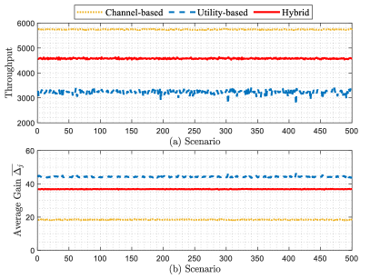
Figure 2: (a) The throughput and (b) the relative information utility gain of communication networks under different policies in different scenarios (data-driven decision-making).

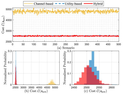
Figure 3: (a) The decision cost under different policies in different scenarios; (b) the probability distribution of decision cost for the $500$ scenarios for three policies; (c) the probability distribution of decision cost for the $500$ scenarios for utility-based and hybrid based policies (data-driven decision making).

We simulate the ED data collection in $500$ scenarios, each presenting a different channel gain for each ED. For the 500 scenarios, the throughput and the relative information utility gain are shown in Fig.2(a) and Fig.2(b), respectively. The throughput is measured as the number of EDs that are scheduled to upload their data. Notably, the channel-based policy achieves the maximum throughput while delivering minimum mean information utility gain. In contrast, the utility-based policy achieves the maximum mean information utility gain while throughput performance is poor. The hybrid policy delivers mediate performance between the two.

The goal of the CPS operator is to bring down the decision costs. In each scenario, upon acquiring the new data $\boldsymbol{z}_{\mathrm{new}}$, we solve the optimization problem described in Eqs.(13)-(15). The cost $\mathcal{C}(\boldsymbol{z}_{\mathrm{new}})$ under different scenarios are depicted in Fig.3(a-c). From Fig.2(a-b), it is noteworthy that the channel-based policy fails to guarantee a low decision cost. The system costs under both the utility-based policy and the hybrid policy are close to each other. Fig.3(c) shows that the hybrid policy can guarantee lower system cost than the utility-based policy. The hybrid policy achieves a balance between the data volume and data utility. Compared with the channel-based policy, the hybrid policy can reduce approximately $50\%$ of possible decision costs under the same communication budget.

V-C Edge Learning

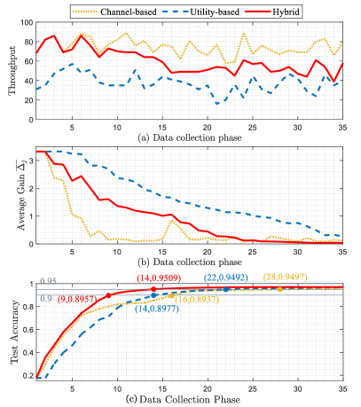
Figure 4: (a) The throughput and (b) the relative information utility gain of communication networks under different policies in different data collection rounds (edge learning). (c) The test accuracy under different data collection rounds. The marked points denote the points that are closest to the $0.9$ and $0.95$ accuracy level line. The numbers in the bracket denote (data collection round, test accuracy).

We conducted edge learning simulations across $35$ phases of data collection. Initially, the server possesses no data samples. For each phase, it collects new data and retrains the learning model. For the 35 phases of data communication, the throughput and the relative information utility gain are shown in Fig.4(a) and Fig.4(b), respectively. The throughput is measured as the number of raw data samples/images that are uploaded to the edge server. The policies behave in a similar fashion as those in the data-driven decision-making case.

The goal of the CPS operator is to minimize loss function and enhance model accuracy. In each data collection phase, we test the inference accuracy of the model on the test set, and the result is shown in Fig.4(c). In Fig.4(c), we also marked when the test accuracy under three different policies comes closest to the accuracy $0.9$ and $0.95$. In the initial phase, the advantages of abundant data might surpass those of valuable data. The test accuracy under the hybrid policy and the channel-based policy are close to each other. However, as the dataset accumulates, the benefit of useful data may suppress the benefit of more data. Hence, the utility-based policy’s test accuracy surpasses the channel-based ones. Nevertheless, the test accuracy of the hybrid policy consistently leads. Compared with channel-based RBA, the hybrid policy saves approximately $50\%$ of iteration rounds (total training time) to reach $0.9$ and $0.95$ test accuracy.

V-D Federated Learning

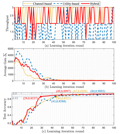
Figure 5: (a) The throughput and (b) the relative information utility gain of communication networks under different policies in different learning iteration rounds (federated learning). (c) The test accuracy under different different learning iteration rounds. The marked points denote the points that are closest to the $0.9$ and $0.95$ accuracy level line. The numbers in the bracket denote (iteration round, test accuracy).

We simulate federated learning over a total of 100 iteration rounds. The server begins with an initial weight. In each round, the operator aggregates the ED gradients and performs gradient descent updates. For the 100 iteration rounds, the throughput and the relative information utility gain are shown in Fig.5(a) and Fig.5(b), respectively. The throughput is measured as the number of EDs that uploaded their gradients to the edge server. The policies demonstrate trends analogous to those in the data-driven decision-making case.

The goal of the CPS operator is to reduce the loss function and enhance model accuracy. In each learning round, we test the inference accuracy of the model on the test set and record the loss function value, shown in Fig.5(c). In Fig.5(c), we also highlight when the test accuracy under three different policies approaches accuracy $0.9$ and $0.95$. Federated learning performs similarly to edge learning. In the initial phase, the benefit of more gradient information may provide more accurate gradient descent information. The test accuracy under the hybrid policy and the channel-based policy are close to each other. However, as the dataset accumulates, the benefit of high-norm gradient information may suppress the benefit of more gradient information. This might stem from the model is already around its convergence region. The crucial aspect is identifying the steepest direction towards the minimum. Compared with the channel-based policy, the hybrid policy can reduce approximately $30\%$ of total training time to reach $0.9$ and $0.95$ test accuracy under the same communication budget.

V-E Distributed Optimization

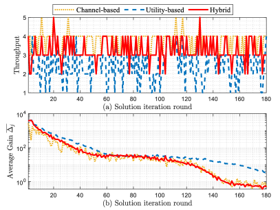
Figure 6: (a) The throughput and (b) the relative information utility gain of communication networks under different policies in different solution iteration rounds (distributed optimization).

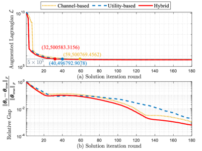
Figure 7: (a) The value of the augmented Lagrangian function and (b) the relative gap under different learning solution rounds. The marked points denote the points that are closest to the $5\times 10^{5}$ level line. The numbers in the bracket denote (iteration round, Lagrangian function value).

We conducted simulations of the distributed system identification over a total of 180 iteration rounds. All the EDs and the server start with an initial guess $\boldsymbol{\theta}=\bf{0}$. For the 180 iteration rounds, the throughput and the relative information utility gain are shown in Fig.6(a) and Fig.6(b), respectively. The throughput is measured as the number of EDs that uploaded their primal variables and dual variables to the server. The observed policy trends align with the data-driven decision-making application. Here, the information utility gain under the hybrid policy is close to that of the channel-based policy.

The goal of the CPS operator is to identify the true system matrix $\boldsymbol{\theta}_{\mathrm{true}}$. In each round, we compute the value of the augmented Lagrangian function and relative gap between the server estimated matrix $\boldsymbol{\theta}_{0}$ and the true system matrix $\boldsymbol{\theta}_{\mathrm{true}}$. The result is shown in Fig.7(a)-(b). It’s evident that the hybrid approach contributes to reductions in both the Lagrangian function and the optimality gap. However, concerning the gap between the estimated matrix and the real matrix, the utility-based policy does not perform so well compared with the channel-based approach. In this case, the importance of more frequent updates could be more important. The consensus update will be slow if the central node estimation cannot gather enough information. Compared with the channel-based policy, the hybrid policy can reduce approximately $30\%$ of iteration time to reach $10^{-3}$ relative optimality gap under the same communication budget.

VI Conclusion

In this study, we presented a novel goal-oriented RBA framework tailored for future CPSs, termed as ‘goal-oriented communications’. Distinct from traditional communication resource allocation methods, this approach prioritizes information transmission essential to CPS goals over purely transmission-centric goals. This paradigm is poised to gain prominence, especially as communication devices evolve to predominantly encompass massive machines and things rather than humans. We conducted simulations encompassing typical use cases of CPSs. These simulations validate the efficacy of our proposed goal-oriented RBA strategy, which considers both information utility and channel conditions.

Future research could explore more applications like transient control of digital twin systems in CPSs, where the requirements for delay and reliability are more stringent. Furthermore, if allowed, a co-design framework for CPS operation and communication can be developed, which can further increase the system’s efficiency.

Appendix

VI-A Proof for Proposition 9

Before proving proposition 9, we first provide the lemmas below:

Assumption 2.

The individual loss function $L_{j}(\mathsf{z}_{j};\boldsymbol{\theta}_{j})$ is convex and $\kappa_{j}$-smooth.

Definition 1.

A differentiable function $f(\boldsymbol{x})$ is called $\rho$ strongly-convex if $\nabla^{2}f(\boldsymbol{x})\succeq\rho\mathbf{I}$. For $\rho$ strongly convex functions, the following is true:

$$f(\boldsymbol{x}^{\prime})\geq f(\boldsymbol{x})+\langle\nabla f(\boldsymbol{x}),\boldsymbol{x}^{\prime}-\boldsymbol{x}\rangle+\frac{\rho}{2}\|\boldsymbol{x}^{\prime}-\boldsymbol{x}\|_{2}^{2},\forall\boldsymbol{x}^{\prime},\boldsymbol{x}$$ (42)

Lemma 3.

The augmented Lagrangian function $\mathcal{L}\left(\boldsymbol{\theta}_{0},\boldsymbol{\theta}_{j},\boldsymbol{\lambda}_{j}\right)$ is $\rho$ strongly convex with respect to $\boldsymbol{\theta}_{0}$ and $\boldsymbol{\theta}_{j}$, respectively.

Proof.

It is easy to verify that:

$$\nabla_{\boldsymbol{\theta}_{j}}^{2}\mathcal{L}=\nabla_{\boldsymbol{\theta}_{j}}^{2}L_{j}+\rho\mathbf{I}\succeq\rho\mathbf{I},~{}~{}\nabla_{\boldsymbol{\theta}_{0}}^{2}\mathcal{L}=\rho\mathbf{I}\succeq\rho\mathbf{I}$$ (43)

where $\nabla_{\boldsymbol{\theta}_{j}}^{2}L_{j}\succeq\mathbf{0}$ because $L_{j}(\mathsf{z}_{j};\boldsymbol{\theta}_{j})$ is convex. ∎

Lemma 4.

The dual variable updates for two consecutive rounds can be bounded as follows:

$$\left\|\boldsymbol{\lambda}_{j,k+1}-\boldsymbol{\lambda}_{j,k}\right\|_{2}\leqslant\kappa_{j}\left\|\boldsymbol{\theta}_{j,k+1}-\boldsymbol{\theta}_{j,k}\right\|_{2}$$ (44)

Proof.

For EDs that take part in updates in round $s_{j}=1$. $\boldsymbol{\vartheta}_{j,k+1}$ is the solution to problem (35) and thus it satisfies the following optimality condition:

$$\nabla_{\boldsymbol{\theta}_{j}}L_{j}\mid_{\boldsymbol{\theta}_{j,k+1}}+\boldsymbol{\lambda}_{j,k}+\rho\left(\boldsymbol{\theta}_{j,k+1}-\boldsymbol{\theta}_{0,k+1}\right)=0$$ (45)

Combing the dual update step (36), we get:

$$\nabla_{\boldsymbol{\theta}_{j}}L_{j}\mid_{\boldsymbol{\theta}_{j,k+1}}=-\boldsymbol{\lambda}_{j,k+1}$$ (46)

Thereby, we have:

$$\left\|\boldsymbol{\lambda}_{j,k+1}-\boldsymbol{\lambda}_{j,k}\right\|_{2} =\left\|\nabla_{\boldsymbol{\theta}_{j}}L_{j}\mid_{\boldsymbol{\theta}_{j,k+1}}-\nabla_{\boldsymbol{\theta}_{j}}L_{j}\mid_{\boldsymbol{\theta}_{j,k}}\right\|_{2}$$ (47)

$$\leqslant\kappa_{j}\left\|\boldsymbol{\theta}_{j,k+1}-\boldsymbol{\theta}_{j,k}\right\|_{2}$$

where the inequality stems from the $\kappa_{j}$-smooth condition. For $j\notin\{j|s_{j}=1\}$, the inequality is trivial because both sides are zero. ∎

Now, we are ready to prove proposition 9.

Proof.

The changes in Lagrangian function are decomposed into three parts:

$$\mathcal{L}\left(\boldsymbol{\theta}_{0,k+1},\boldsymbol{\theta}_{j,k+1},\boldsymbol{\lambda}_{j,k+1}\right)-\mathcal{L}\left(\boldsymbol{\theta}_{0,k},\boldsymbol{\theta}_{j,k},\boldsymbol{\lambda}_{j,k}\right)$$ (48)

$$= \mathcal{L}\left(\boldsymbol{\theta}_{0,k+1},\boldsymbol{\theta}_{j,k+1},\boldsymbol{\lambda}_{j,k+1}\right)-\mathcal{L}\left(\boldsymbol{\theta}_{0,k+1},\boldsymbol{\theta}_{j,k+1},\boldsymbol{\lambda}_{j,k}\right)$$

$$+ \mathcal{L}\left(\boldsymbol{\theta}_{0,k+1},\boldsymbol{\theta}_{j,k+1},\boldsymbol{\lambda}_{j,k}\right)-\mathcal{L}\left(\boldsymbol{\theta}_{0,k+1},\boldsymbol{\theta}_{j,k},\boldsymbol{\lambda}_{j,k}\right)$$

$$+ \mathcal{L}\left(\boldsymbol{\theta}_{0,k+1},\boldsymbol{\theta}_{j,k},\boldsymbol{\lambda}_{j,k}\right)-\mathcal{L}\left(\boldsymbol{\theta}_{0,k},\boldsymbol{\theta}_{j,k},\boldsymbol{\lambda}_{j,k}\right)$$

The first part can be computed as follows:

$$\mathcal{L}\left(\boldsymbol{\theta}_{0,k+1},\boldsymbol{\theta}_{j,k+1},\boldsymbol{\lambda}_{j,k+1}\right)-\mathcal{L}\left(\boldsymbol{\theta}_{0,k+1},\boldsymbol{\theta}_{j,k+1},\boldsymbol{\lambda}_{j,k}\right)$$ (49)

$$\overset{\left(\mathrm{I}\right)}{=} \sum\nolimits_{j}{\left<\boldsymbol{\lambda}_{j,k+1}-\boldsymbol{\lambda}_{j,k},\boldsymbol{\theta}_{j,k+1}-\boldsymbol{\theta}_{0,k+1}\right>}$$

$$\overset{\left(\mathrm{II}\right)}{=} \sum\nolimits_{j\in\{j|s_{j}=1\}}{\frac{1}{\rho}\left\|\boldsymbol{\lambda}_{j,k+1}-\boldsymbol{\lambda}_{j,k}\right\|_{2}^{2}}$$

In $(\mathrm{I})$, the expression of the Lagrangian function is used. In $(\mathrm{II})$, the update law of dual multipliers step (36) is used. Besides, for $j\notin\{j|s_{j}=1\}$, $\boldsymbol{\lambda}_{j,k+1}-\boldsymbol{\lambda}_{j,k}=0$.

The second part can be bounded as follows:

$$\mathcal{L}\left(\boldsymbol{\theta}_{0,k+1},\boldsymbol{\theta}_{j,k+1},\boldsymbol{\lambda}_{j,k}\right)-\mathcal{L}\left(\boldsymbol{\theta}_{0,k+1},\boldsymbol{\theta}_{j,k},\boldsymbol{\lambda}_{j,k}\right)$$ (50)

$$\overset{(\mathrm{I})}{\leqslant} \sum_{j}{\left.\langle\left.\nabla_{\boldsymbol{\theta}_{j}}\mathcal{L}\right|_{\boldsymbol{\theta}_{j,k+1}},\boldsymbol{\theta}_{j,k+1}-\boldsymbol{\theta}_{j,k}\right.}\rangle-\frac{\rho}{2}\left\|\boldsymbol{\theta}_{j,k+1}-\boldsymbol{\theta}_{j,k}\right\|_{2}^{2}$$

$$\overset{\left(\mathrm{II}\right)}{\leqslant} \sum_{j\in\{j|s_{j}=1\}}{\left.\langle\left.\nabla_{\boldsymbol{\theta}_{j}}\mathcal{L}\right|_{\boldsymbol{\theta}_{j,k+1}},\boldsymbol{\theta}_{j,k+1}-\boldsymbol{\theta}_{j,k}\right.}\rangle-\frac{\rho}{2}\left\|\boldsymbol{\theta}_{j,k+1}-\boldsymbol{\theta}_{j,k}\right\|_{2}^{2}$$

$$\overset{\left(\mathrm{III}\right)}{\leqslant} -\sum_{j\in\{j|s_{j}=1\}}{\frac{\rho}{2}}\left\|\boldsymbol{\theta}_{j,k+1}-\boldsymbol{\theta}_{j,k}\right\|_{2}^{2}$$

In $(\mathrm{I})$, the property of strongly convex is used when $\boldsymbol{\theta}_{j}=\boldsymbol{\theta}_{j,k+1}$. In $(\mathrm{II})$, we use the fact that $\boldsymbol{\theta}_{j,k+1}-\boldsymbol{\theta}_{j,k}=0$ for $j\notin\{j|s_{j}=1\}$. In $(\mathrm{III})$, the optimal condition of the decomposed sub-problem (35) is used.

The third part can be bounded as follows:

$$\mathcal{L}\left(\boldsymbol{\theta}_{0,k+1},\boldsymbol{\theta}_{j,k},\boldsymbol{\lambda}_{j,k}\right)-\mathcal{L}\left(\boldsymbol{\theta}_{0,k},\boldsymbol{\theta}_{j,k},\boldsymbol{\lambda}_{j,k}\right)$$ (51)

$$\overset{\left(\mathrm{i}\right)}{\leqslant} \left.\langle\left.\nabla_{\boldsymbol{\theta}_{0}}\mathcal{L}\right|_{\boldsymbol{\theta}_{0,k+1}},\boldsymbol{\theta}_{0,k+1}-\boldsymbol{\theta}_{0,k}\right.\rangle-\frac{\rho}{2}\left\|\boldsymbol{\theta}_{0,k+1}-\boldsymbol{\theta}_{0,k}\right\|_{2}^{2}$$

$$\overset{\left(\mathrm{II}\right)}{\leqslant} -\frac{\rho}{2}\left\|\boldsymbol{\theta}_{0,k+1}-\boldsymbol{\theta}_{0,k}\right\|_{2}^{2}$$

In $(\mathrm{I})$, the property of strongly convex is used when $\boldsymbol{\theta}_{0}=\boldsymbol{\theta}_{0,k+1}$. In $(\mathrm{II})$, the optimal condition of the decomposed sub-problem (34) is used.

Combining the three parts above:

$$\mathcal{L}\left(\boldsymbol{\theta}_{0,k+1},\boldsymbol{\theta}_{j,k+1},\boldsymbol{\lambda}_{j,k+1}\right)-\mathcal{L}\left(\boldsymbol{\theta}_{0,k},\boldsymbol{\theta}_{j,k},\boldsymbol{\lambda}_{j,k}\right)$$ (52)

$$\leqslant -\sum_{j\in\{j|s_{j}=1\}}{\frac{\rho}{2}\left\|\boldsymbol{\theta}_{j,k+1}-\boldsymbol{\theta}_{j,k}\right\|_{2}^{2}}-\frac{\rho}{2}\left\|\boldsymbol{\theta}_{0,k+1}-\boldsymbol{\theta}_{0,k}\right\|_{2}^{2}$$

$$+\sum_{j\in\{j|s_{j}=1\}}{\frac{1}{\rho}\left\|\boldsymbol{\lambda}_{j,k+1}-\boldsymbol{\lambda}_{j,k}\right\|_{2}^{2}}$$

$$\overset{\left(\mathrm{I}\right)}{\leqslant} -\sum\nolimits_{j\in\{j|s_{j}=1\}}{\left(\frac{\rho}{2}-\frac{\kappa_{j}}{\rho}\right)\left\|\boldsymbol{\theta}_{j,k+1}-\boldsymbol{\theta}_{j,k}\right\|_{2}^{2}}$$

$$-\frac{\rho}{2}\left\|\boldsymbol{\theta}_{0,k+1}-\boldsymbol{\theta}_{0,k}\right\|_{2}^{2}$$

where in (I), we use lemma 4. Thereby, when $\rho$ is sufficiently large, we can guarantee the Lagrangian is always reducing. Replace the coefficients and we get proposition 4. ∎

References

- [1] S. Bi, R. Zhang, Z. Ding, and S. Cui, “Wireless communications in the era of big data,” IEEE communications magazine, vol. 53, no. 10, pp. 190–199, 2015.
- [2] A. Humayed, J. Lin, F. Li, and B. Luo, “Cyber-physical systems security—a survey,” IEEE Internet of Things Journal, vol. 4, no. 6, pp. 1802–1831, 2017.
- [3] Z. Dawy, W. Saad, A. Ghosh, J. G. Andrews, and E. Yaacoub, “Toward massive machine type cellular communications,” IEEE Wireless Communications, vol. 24, no. 1, pp. 120–128, 2016.
- [4] Q. Lan, D. Wen, Z. Zhang, Q. Zeng, X. Chen, P. Popovski, and K. Huang, “What is semantic communication? a view on conveying meaning in the era of machine intelligence,” Journal of Communications and Information Networks, vol. 6, no. 4, pp. 336–371, 2021.
- [5] E. Uysal, O. Kaya, A. Ephremides, J. Gross, M. Codreanu, P. Popovski, M. Assaad, G. Liva, A. Munari, B. Soret et al., “Semantic communications in networked systems: A data significance perspective,” IEEE Network, vol. 36, no. 4, pp. 233–240, 2022.
- [6] Z. Qin, X. Tao, J. Lu, W. Tong, and G. Y. Li, “Semantic communications: Principles and challenges,” arXiv preprint arXiv:2201.01389, 2021.
- [7] A. Burg, A. Chattopadhyay, and K.-Y. Lam, “Wireless communication and security issues for cyber–physical systems and the internet-of-things,” Proceedings of the IEEE, vol. 106, no. 1, pp. 38–60, 2017.
- [8] X. Yu and Y. Xue, “Smart grids: A cyber–physical systems perspective,” Proceedings of the IEEE, vol. 104, no. 5, pp. 1058–1070, 2016.
- [9] Y. Zhang, T. Jiang, Q. Shi, W. Liu, and S. Huang, “Modeling and vulnerability assessment of cyber physical system considering coupling characteristics,” International Journal of Electrical Power & Energy Systems, vol. 142, p. 108321, 2022.
- [10] A. Mostaani, T. X. Vu, S. K. Sharma, V.-D. Nguyen, Q. Liao, and S. Chatzinotas, “Task-oriented communication design in cyber-physical systems: A survey on theory and applications,” IEEE Access, vol. 10, pp. 133 842–133 868, 2022.
- [11] E. A. Coelho, D. Wu, J. M. Guerrero, J. C. Vasquez, T. Dragicević, C. Stefanović, and P. Popovski, “Small-signal analysis of the microgrid secondary control considering a communication time delay,” IEEE Transactions on Industrial Electronics, vol. 63, no. 10, pp. 6257–6269, 2016.
- [12] L. Zheng, N. Lu, and L. Cai, “Reliable wireless communication networks for demand response control,” IEEE Transactions on Smart Grid, vol. 4, no. 1, pp. 133–140, 2013.
- [13] T. Yang, J. Lu, D. Wu, J. Wu, G. Shi, Z. Meng, and K. H. Johansson, “A distributed algorithm for economic dispatch over time-varying directed networks with delays,” IEEE Transactions on Industrial Electronics, vol. 64, no. 6, pp. 5095–5106, 2017.
- [14] M. H. Nazari, L. Y. Wang, S. Grijalva, and M. Egerstedt, “Communication-failure-resilient distributed frequency control in smart grids: Part i: Architecture and distributed algorithms,” IEEE Transactions on Power Systems, vol. 35, no. 2, pp. 1317–1326, 2020.
- [15] H. Liang, B. J. Choi, W. Zhuang, and X. Shen, “Stability enhancement of decentralized inverter control through wireless communications in microgrids,” IEEE Transactions on Smart Grid, vol. 4, no. 1, pp. 321–331, 2013.
- [16] M. Rabbat and R. Nowak, “Quantized incremental algorithms for distributed optimization,” IEEE Journal on Selected Areas in Communications, vol. 23, no. 4, pp. 798–808, 2005.
- [17] X. Liu, L. Li, Z. Li, X. Chen, T. Fernando, H. H.-C. Iu, and G. He, “Event-trigger particle filter for smart grids with limited communication bandwidth infrastructure,” IEEE Transactions on Smart Grid, vol. 9, no. 6, pp. 6918–6928, 2017.
- [18] A. S. Berahas, R. Bollapragada, N. S. Keskar, and E. Wei, “Balancing communication and computation in distributed optimization,” IEEE Transactions on Automatic Control, vol. 64, no. 8, pp. 3141–3155, 2018.
- [19] X. Luo, H.-H. Chen, and Q. Guo, “Semantic communications: Overview, open issues, and future research directions,” IEEE Wireless Communications, vol. 29, no. 1, pp. 210–219, 2022.
- [20] W. Yang, H. Du, Z. Q. Liew, W. Y. B. Lim, Z. Xiong, D. Niyato, X. Chi, X. Shen, and C. Miao, “Semantic communications for future internet: Fundamentals, applications, and challenges,” IEEE Communications Surveys & Tutorials, vol. 25, no. 1, pp. 213–250, 2023.
- [21] Y. Shi, Y. Zhou, D. Wen, Y. Wu, C. Jiang, and K. B. Letaief, “Task-oriented communications for 6g: Vision, principles, and technologies,” arXiv preprint arXiv:2303.10920, 2023.
- [22] D. Gündüz, Z. Qin, I. E. Aguerri, H. S. Dhillon, Z. Yang, A. Yener, K. K. Wong, and C.-B. Chae, “Beyond transmitting bits: Context, semantics, and task-oriented communications,” IEEE Journal on Selected Areas in Communications, vol. 41, no. 1, pp. 5–41, 2023.
- [23] E. C. Strinati and S. Barbarossa, “6g networks: Beyond shannon towards semantic and goal-oriented communications,” Computer Networks, vol. 190, p. 107930, 2021.
- [24] H. Xie, Z. Qin, X. Tao, and K. B. Letaief, “Task-oriented multi-user semantic communications,” IEEE Journal on Selected Areas in Communications, vol. 40, no. 9, pp. 2584–2597, 2022.
- [25] S. Xie, S. Ma, M. Ding, Y. Shi, M. Tang, and Y. Wu, “Robust information bottleneck for task-oriented communication with digital modulation,” IEEE Journal on Selected Areas in Communications, vol. 41, no. 8, pp. 2577–2591, 2023.
- [26] Q. Lan, D. Wen, Z. Zhang, Q. Zeng, X. Chen, P. Popovski, and K. Huang, “What is semantic communication? a view on conveying meaning in the era of machine intelligence,” Journal of Communications and Information Networks, vol. 6, no. 4, pp. 336–371, 2021.
- [27] H. Xie, Z. Qin, G. Y. Li, and B.-H. Juang, “Deep learning enabled semantic communication systems,” IEEE Transactions on Signal Processing, vol. 69, pp. 2663–2675, 2021.
- [28] J. Shao, Y. Mao, and J. Zhang, “Learning task-oriented communication for edge inference: An information bottleneck approach,” IEEE Journal on Selected Areas in Communications, vol. 40, no. 1, pp. 197–211, 2021.
- [29] J. Park, S. Samarakoon, A. Elgabli, J. Kim, M. Bennis, S.-L. Kim, and M. Debbah, “Communication-efficient and distributed learning over wireless networks: Principles and applications,” Proceedings of the IEEE, vol. 109, no. 5, pp. 796–819, 2021.
- [30] Y. Shi, K. Yang, T. Jiang, J. Zhang, and K. B. Letaief, “Communication-efficient edge ai: Algorithms and systems,” IEEE Communications Surveys & Tutorials, vol. 22, no. 4, pp. 2167–2191, 2020.
- [31] D. Liu, G. Zhu, J. Zhang, and K. Huang, “Data-importance aware user scheduling for communication-efficient edge machine learning,” IEEE Transactions on Cognitive Communications and Networking, vol. 7, no. 1, pp. 265–278, 2020.
- [32] S. Niknam, H. S. Dhillon, and J. H. Reed, “Federated learning for wireless communications: Motivation, opportunities, and challenges,” IEEE Communications Magazine, vol. 58, no. 6, pp. 46–51, 2020.
- [33] M. Chen, N. Shlezinger, H. V. Poor, Y. C. Eldar, and S. Cui, “Communication-efficient federated learning,” Proceedings of the National Academy of Sciences, vol. 118, no. 17, p. e2024789118, 2021.
- [34] M. M. Amiri, D. Gündüz, S. R. Kulkarni, and H. V. Poor, “Convergence of update aware device scheduling for federated learning at the wireless edge,” IEEE Transactions on Wireless Communications, vol. 20, no. 6, pp. 3643–3658, 2021.
- [35] W. Shi, S. Zhou, Z. Niu, M. Jiang, and L. Geng, “Joint device scheduling and resource allocation for latency constrained wireless federated learning,” IEEE Transactions on Wireless Communications, vol. 20, no. 1, pp. 453–467, 2020.
- [36] T. Roughgarden, Twenty Lectures on Algorithmic Game Theory. Cambridge University Press, 2016.
- [37] B. Settles, Active Learning, ser. Synthesis Lectures on Artificial Intelligence and Machine Learning. Morgan & Claypool Publishers, 2012.
- [38] S. Boyd, N. Parikh, E. Chu, B. Peleato, J. Eckstein et al., “Distributed optimization and statistical learning via the alternating direction method of multipliers,” Foundations and Trends® in Machine learning, vol. 3, no. 1, pp. 1–122, 2011.
- [39] Z. Han, X. Li, Z. Zhou, K. Huang, Y. Gong, and Q. Zhang, “Wireless communication and control co-design for system identification,” IEEE Transactions on Wireless Communications, pp. 1–1, 2023.
- [40] Y. Sun, S. Zhou, Z. Niu, and D. Gündüz, “Dynamic scheduling for over-the-air federated edge learning with energy constraints,” IEEE Journal on Selected Areas in Communications, vol. 40, no. 1, pp. 227–242, 2022.