Abstract

Graph Neural Networks (GNNs) offer a compact and computationally efficient way to learn embeddings and classifications on graph data. GNN models are frequently large, making distributed minibatch training necessary.

The primary contribution of this paper is new methods for reducing communication in the sampling step for distributed GNN training. Here, we propose a matrix-based bulk sampling approach that expresses sampling as a sparse matrix multiplication (SpGEMM) and samples multiple minibatches at once. When the input graph topology does not fit on a single device, our method distributes the graph and use communication-avoiding SpGEMM algorithms to scale GNN minibatch sampling, enabling GNN training on much larger graphs than those that can fit into a single device memory. When the input graph topology (but not the embeddings) fits in the memory of one GPU, our approach (1) performs sampling without communication, (2) amortizes the overheads of sampling a minibatch, and (3) can represent multiple sampling algorithms by simply using different matrix constructions. In addition to new methods for sampling, we show that judiciously replicating feature data with a simple all-to-all exchange can outperform current methods for the feature extraction step in distributed GNN training. We provide experimental results on the largest Open Graph Benchmark (OGB) datasets on $128$ GPUs, and show that our pipeline is $2.5\times$ faster Quiver (a distributed extension to PyTorch-Geometric) on a $3$-layer GraphSAGE network. On datasets outside of OGB, we show a $8.46\times$ speedup on $128$ GPUs in-per epoch time. Finally, we show scaling when the graph is distributed across GPUs and scaling for both node-wise and layer-wise sampling algorithms.

1 Introduction

Graph Neural Networks (GNNs) are a class of neural networks increasingly used for scientific and industrial problems including protein family classification in proteomics, track reconstruction in particle tracking, and fraud detection Wu et al. (2020)

Training GNNs requires sampling minibatches from the training set. Minibatch training is more common than full-batch because it yields faster time-to-convergence and higher accuracy. For node classification, however, sampling batches is more complex than other deep learning (DL) problems since vertices in a batches have edges to vertices outside the batch. Training each batch of vertices for an $L$-layer GNN accesses the entire $L$-hop neighborhood of the batch (neighborhood explosion), which is prohibitively expensive for many real-world graphs.

Many have proposed algorithms that sample from the $L$-hop neighborhood of a minibatch. These algorithms are necessary, and effectively reduce the time and memory costs to train a single minibatch. Broadly, sampling algorithms can be categorized as either: (1) node-wise, (2) layer-wise, and (3) graph-wise.

Unfortunately, sampling algorithms must be able to access the entire graph, which is oftentimes too large to fit in GPU memory. Current GNN tools, such as Deep Graph Library (DGL) and PyTorch Geometric (PyG), run sampling on CPU as a consequence — a weaker processor compared to GPUs Zheng et al. (2020); Fey & Lenssen (2019). Those that do not, such as Quiver, restrict the graph size by fully replicating the graph on each GPU used. In addition, sampling algorithms are frequently the bottleneck of GNN training when compared to forward and backward propgation, and only GraphSAGE has an existing multi-node implementation. In this work, we propose a method to sample on a graph distributed across GPUs, and show its effectiveness across many types of sampling algorithms.

Distributed and GPU graph analytics is a well-studied field, and expressing graph algorithms in the language of sparse linear algebra is a proven approach Buluç & Gilbert (2011); Yang et al. (2022a). By representing a graph algorithm in terms of matrix operations, one can leverage existing decades of work in distributed sparse matrix algorithms to distribute graph computation.

In this work, we show how to express node-wise and layer-wise sampling algorithms in the language of linear algebra. We propose a matrix-based bulk sampling approach that (1) amortizes the cost of sampling a minibatch, and (2) leverages distributed, communication-avoiding sparse matrix multiplication algorithms for scalability. We also include an optimization for the feature fetching step in distributed GNN training. As a byproduct, we also introduce the first fully distributed implementation of the LADIES algorithm. We provide theoretical and empirical results that outperform existing GNN tools.

2 Background

Table 1: List of symbols and notations used in our pipeline

Symbols and Notations
Symbol	Description
$\mathbf{A}$	Adjacency matrix of graph ($n\times n$)
$\mathbf{H}^{l}$	Embedding matrix in layer $l$ ($n\times f$)
$\mathbf{W}^{l}$	Weight matrix in layer $l$ ($f\times f$)
$\mathbf{Q}^{l}$	Sparse sampler matrix in layer $l$
$\mathbf{P}$	Probability matrix during sampling
$\mathbf{A}_{S}$	Sampled adjacency matrix
$f$	Length of feature vector per vertex
$L$	Total layers in GNN
$p$	Total number of processes
$\alpha$	Latency
$\beta$	Reciprocal bandwidth
$b$	Batch size
$s$	Sampling parameter
$k$	Number of batches to sample in bulk

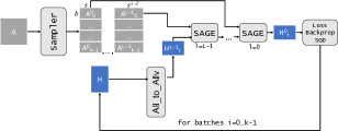
Figure 1: The overall architecture of our distributed pipeline from the perspective of one process. In this diagram, $\mathbf{A}$ is either the entire adjacency matrix or a partition, depending on the algorithm, and $\mathbf{H}$ is a partition of the input feature matrix. The first step in the pipeline is to run sampling on $k$ minibatches at once. Then, for each minibatch, we iteratively call all-to-allv fetch the appropriate feature vectors, and run propagation on minibatch.

2.1 Graph Neural Networks

Graph Neural Networks take as input a graph $G=(V,E)$. While GNNs can solve a wide variety of machine learning problems, we focus on node classification without loss of generality. In this problem, each vertex takes an associated feature vector as input, and a subset of vertices have an associated label. The objective of the network is to classify unlabelled vertices in the graph using input features, graph connectivity, and vertex labels.

GNNs follow the message-passing model, consisting of a message step and an aggregate step per iteration of training Hamilton et al. (2017). The message step creates a message per edge in the graph. The aggregate step takes a vertex $v$ and combines the messages across all of that $v$’s incoming neighbors. The output is multiplied with a parameter weight matrix, and the result is an embedding vector $z_{v}$. After several layers of both steps, the network outputs an embedding vector per vertex, after which the network inputs vectors and labels into a loss function for backpropagation. Formally, for an arbitrary layer $l$, computing an embedding vector $z^{l}_{v}$ is

$$z^{l}_{v}=\text{AGG}(\text{MSG}(z^{l-1}_{u},z^{l-1}_{v}))\forall u\in N(v)$$

$$z^{l}_{v}=z^{l}_{v}\mathbf{W}^{l}$$

While the size of the batch is small compared to the vertex set, running message-passing on a batch naively touches a large fraction of the input graph. Training a batch $B$ in an $L$-layer network requires accessing the $L$-hop aggregated neighborhood of $B$. In scale-free graphs, the $L$-hop neighborhood for a batch would be the entire graph for even small values of $L$. This phenomenon is referred to as neighborhood explosion. The graph in Figure 2, for instance, will touch every vertex in one layer with the batch $B=\{1,5\}$. To alleviate costs, minibatch training GNNs includes a sampling step that samples the $L$-hop neighborhood of each batch. Message-passing on a sampled batch will only aggregate from vertices in its sampled $L$-hop neighborhood. The specific sampling algorithm depends on the problem, and there are many such algorithms in the literature. In addition, in our notation, the $L$-th layer contains the batch vertices, and the 1st layer has vertices furthest from the batch vertices.

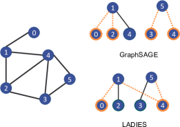
Figure 2: Example outputs for both GraphSAGE and LADIES sampling on a batch with vertices $\{1,5\}$ and a sample number of $s=2$. Bolded vertices denote vertices included in the sample, and dashed edges denote edges included in the sample.

2.2 Sampling Algorithms

GNN sampling algorithms and broadly be classified into three taxonomies: 1) node-wise sampling, 2) layer-wise sampling, and 3) graph-wise sampling. We primarily focus on node-wise and layer-wise sampling in this work. Each category of algorithms have tradeoffs when used, and each category has many algorithms. The algorithm that yields the highest accuracy is highly dependent on the downstream problem. Thus, all of these algorithms are used in some contexts. We explain each type of algorithm in its appropriate subsection, along with the tradeoffs of each approach.

2.2.1 Node-wise sampling

Node-wise algorithms sample from an $L$-hop neighorhood by sampling vertices in the $L$-hop neighborhood of each individual batch vertex.

GraphSAGE

: GraphSAGE is the simplest and most widely used example of node-wise sampling Hamilton et al. (2017). In GraphSAGE, each vertex in the batch samples $s$ of its neighbors as the next layer in the batch uniformly at random. The sample number, $s$, is a hyperparameter. For a multi-layer GNN, each vertex in a layer will sample $s$ of its neighbors for the next layer as well. Figure 2 illustrates this for the example graph and $s=2$. GraphSAGE is a simple algorithm that is straightforward to implement. In our work, we show how our linear algebraic sampling framework expresses node-wise sampling by implementing GraphSAGE.

2.2.2 Layer-wise sampling

Layer-wise algorithms sample from an $L$-hop neighborhood by sampling a set of vertices $S^{l}\subset V$ per layer, and including every edge between $S^{l+1}$ and $S$. The simplest layer-wise sampling algorithm is FastGCN Chen et al. (2018). FastGCN samples $s$ vertices from $V$, where each vertex is sampled with a probability correlated with its degree in $G$. The benefit of FastGCN is it avoids any neighborhood explosion, since the number of vertices in a layer is constrained to $s$. However, computing the probability distribution is an expensive step. In addition, note that vertices in $S$ are not necessarily in the aggregated neighborhood of $S^{l+1}$, which affects accuracy when training with FastGCN.

LADIES

Zou et. al. introduce Layer-Wise Dependency Sampling (LADIES) to ensure only vertices in the aggregated neighborhood of the previous layer are sampled Zou et al. (2019). The algorithm sets the probability a vertex is selected to be correlated with the number of neighbors it has in $S^{l}$. If $e_{v}$ is the number of neighbors vertex $v$ has in $S$, then the probability $v$ is sampled is

$$p_{v}=\frac{e_{v}^{2}}{\sum_{u\in V}e_{u}^{2}}$$

In Figure 2, for a batch $\{1,5\}$, the probability array for all $6$ vertices is

$$\Big{[}\frac{1}{7},0,\frac{1}{7},\frac{1}{7},\frac{4}{7},0\Big{]}$$ (1)

In the example, we have $s=2$ and sampled vertices $\{0,4\}$. Consequently, the sample for LADIES includes every edge between $\{1,5\}$ and $\{0,4\}$. In our work, we show how our linear algebraic sampling framework expresses layer-wise sampling by implementing LADIES.

2.2.3 Graph-wise sampling

In graph-wise sampling, aggregation for a batch $B$ is restricted to vertices within $B$ itself. GraphSAINT is a simple example of this approach Zeng et al. (2020). In GraphSAINT, vertices are selected to be members of $B$ according to a probability distribution. Then, every layer of the batch only includes vertices in $B$, and the only edges in the batch are the edges in the induced subgraph $G[B]$. Zeng et. al. introduce a variety of distributions for sampling batches Zeng et al. (2020). Cluster-GCN is related approach that first runs METIS partitioning on $G$, and sampled clusters of vertices as minibatches Chiang et al. (2019); Karypis & Kumar (1998).

2.3 Distribution Sampling

All GNN sampling algorithms require sampling $s$ elements from some probability distribution. While there exist many algorithms for distribution sampling, the most common are inverse transform sampling (ITS) and rejection sampling Pandey et al. (2020); Yang et al. (2019); Olver & Townsend (2013); Hübschle-Schneider & Sanders (2022). ITS first runs a prefix sum on the distribution, and samples an element by binary searching a random number $r\in[0,1)$ in the distribution. Rejection sampling, on the other hand, first generates an index $i$ into the distribution, and then generates a random number $r\in[0,1)$. If $r<p_{i}$, element $i$ is selected, and if not, the process is repeated until an element is selected. While rejection sampling avoids a potentially costly prefix sum operation, it risks taking many iterations to complete. In our work, we use ITS, and empirically show the prefix sum is a negligible cost in our problem.

2.4 Notation

Table 1 lists the notations we use in this paper. When we refer to layer $L$, we refer to the last layer in the network with only the vertices in the minibatch. In addition, when analyzing communication costs, we use the $\alpha-\beta$ model. Here, each message takes a constant $\alpha$ time units latency irrespective of its size plus an inverse bandwidth term that takes $\beta$ time units per word in the message to reach its destination. Thus, sending a message of $k$ words takes $\alpha+\beta k$ time.

3 Related Work

3.1 Distributed GNN Systems

Real-world graphs and GNN datasets are frequently too large to fit on a single device, necessitating distributed GNN training. The two most popular GNN training tools are Deep Graph Library (DGL) and PyTorch Geometric (PyG), which can be distributed with Quiver Team (2023). Both DGL and Quiver run most sampling algorithms on CPU with the graph stored in RAM. For node-wise sampling, these tools support sampling with the graph stored on GPU.

In addition to these, there exist many distributed GNN systems for both full-batch and minibatch training. Full-batch training systems include NeuGraph Ma et al. (2019), ROC Jia et al. (2020), AliGraph Zhu et al. (2019), CAGNET, PipeGCN Wan et al. (2022b), BNS-GCN Wan et al. (2022a), and CoFree-GNN Cao et al. (2023). In full-batch distributed GNN training, the graph is typically partitioned across devices, and the main performance bottleneck is communicating vertex embeddings between devices. Each work takes a different approach in reducing this communication.

While full-batch training smoothly approaches minima in the loss landscape, minibatch training tends to achieve better generalization by introducing noise to avoid sharp, local minima. Thus, in this work, we focus on minibatch training. For minibatch training, existing systems include DistDGL Zheng et al. (2020), Quiver, GNNLab Yang et al. (2022c), WholeGraph Yang et al. (2022b), DSP Cai et al. (2023), PGLBox Jiao et al. (2023), SALIENT++ Kaler et al. (2023), NextDoor Jangda et al. (2021), $P^{3}$ Gandhi & Iyer (2021). Here, the main performance bottleneck is the cost of sampling minibatches. Minibatches for GNN node classifcation are sets of vertices, but training a minibatch touches its $L$-hop neighborhood in an $L$-layer network. Thus, most GNN models sample from the $L$-hop neighorhood of a minibatch before training that minibatch. This sampling step is usually the bottleneck of minibatch training due to random memory accesses, difficulty parallelizing, and communicating samples from CPU to GPU, with studies showing that sampling can take up to 60% of the total training time Jangda et al. (2021); Yang et al. (2022c).

Notably, none of the minibatch systems in the current literature achieve all of the following: (1) sample minibatches on GPU, (2) support distributed, multi-node training, and (3) supports multiple sampling algorithms (Table  2). Sampling on GPUs, if possible, is preferred to CPUs as it communicating samples from CPU to GPU over a low-bandwidth link like PCIe. In addition, multi-node training is necessary to train large GNN datasets. Some systems, such as Quiver and WholeGraph, support multi-node training by replicating the graph dataset (topology and embeddings) on each node. While this replication can take advantage of additional compute resources, it still limits the size of the dataset for training. Finally, while most systems support node-wise sampling algorithms, layer-wise and graph-wise sampling algorithms have shown to achieve higher accuracy for certain applications. Supporting multiple types of sampling algorithms on GPU is necessary for a robust GNN training system. To our knowledge, our system would be the first to simultaneously support GPU sampling for minibatches, fully distributed multi-node training, and multiple sampling algorithms.

3.2 Graph Sampling Systems

In addition to GNN systems, many have worked on systems that return samples of an input graph. KnightKing is a distributed CPU-based graph sampler, and C-SAW is a GPU-based graph sampler Yang et al. (2019); Pandey et al. (2020). These systems address the broader problem of graph sampling, while our work is tailored towards sampling algorithms in the context of GNN training.

Table 2: Existing distributed minibatch GNN systems

Distributed Minibatch GNN Systems
System	GPU Sampling	Multi-node Training*	Multiple Samplers
DistDGL	✔	✔
Quiver	✔	✔
GNNLab	✔
WholeGraph	✔
DSP	✔		✔
PGLBox	✔
SALIENT++		✔
NextDoor	✔		✔
$P^{3}$		✔
This work	✔	✔	✔

$*$ does not include systems that require replicating both the graph and features on each node or GPU, as this limits the datasets that can be trained.

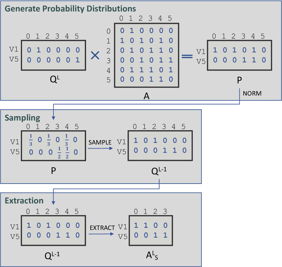
(a) GraphSAGE Operations

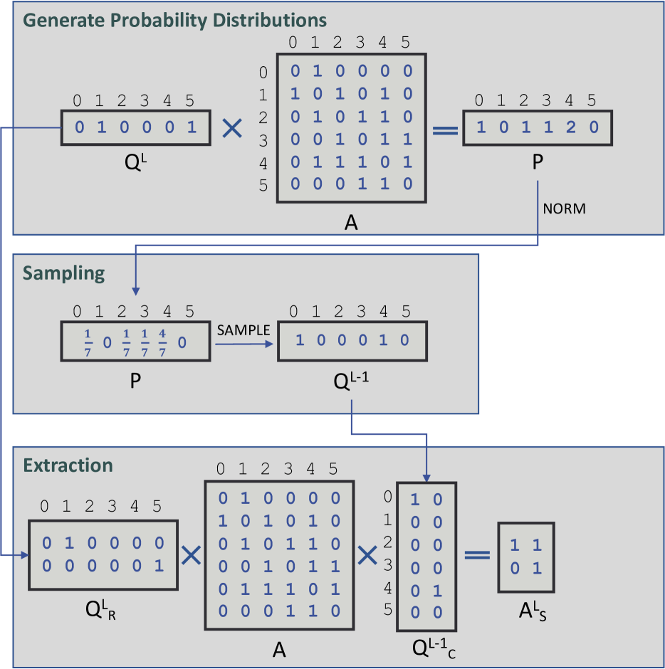
(b) LADIES Operations

Figure 3: Diagram of matrix operations used to sample the first layer of a GNN formed from the example graph in Figure 2 along with the minibatch $\{1,5\}$.

4 Matrix-Based Algorithms for Sampling

In this section, we introduce our approach to represent GraphSAGE and LADIES with matrix operations, and how we use this formulation to sample minibatches in bulk. We first discuss how to sample a single minibatch with our matrix-based approach. Subsequently, we show how to generalize into sampling all minibatches in bulk. We discuss how to distribute these algorithms in Section 5, and only focus on the matrix representations in this section.

Each algorithm takes as input

1. $\mathbf{A}\in\{0,1\}^{n\times n}:$ sparse adjacency matrix,

2. $\mathbf{Q}^{L}:$ sparse sampler-dependent matrix,

3. $b:$ batch size,

4. $s:$ sampling parameter,

The output of sampling is a list of sampled adjacency matrices $\mathbf{A}^{0}\ldots\mathbf{A}^{L-1}$ for a minibatch. Each sampled adjacency matrix $\mathbf{A}^{l}$ is the adjacency matrix used in layer $l$’s aggregation step in forward propagation. $\mathbf{Q}^{L}$ is a sparse matrix that holds the minibatch vertices. The exact structure and dimensions for $\mathbf{Q}^{L}$ is dependent on the sampling algorithm, and will be specified in the respective subsection.

Each algorithm follows the same three-step framework outlined in Figure 3(a) — 1) generate probability distributions to sample from, 2) sample from each distribution, 3) extract rows and columns from the input adjacency matrix. $\mathbf{P}$ holds one distribution per row, and the sampling step reduces to sampling from each row of $\mathbf{P}$. For GraphSAGE, each row of $\mathbf{P}$ is the neighborhood of a batch vertex. For LADIES, each row of $\mathbf{P}$ is the distribution across the aggregated neighborhood of a batch. Once we compute $\mathbf{P}$, we sample $s$ nonzeros per row of $\mathbf{P}$ using Inverse Transform Sampling (ITS). We then extract rows of $\mathbf{A}$ from the vertices sampled in the prior layer ($\mathbf{Q}^{l}$) and columns of $\mathbf{A}$ from the newly sampled vertices ($\mathbf{Q}^{l-1}$). In the respective GraphSAGE and LADIES subsections, we detail the structure for $\mathbf{Q}^{L}$, and the matrix operations used to implement each function called in Algorithm 1.

Algorithm 1 Matrix-based abstraction for sampling algorithms. Each algorithm implements the NORM and EXTRACT functions. SAMPLE uses Inverse Transform Sampling.

1:  for $l=L$ to $1$ do

2:     $\mathbf{P}\leftarrow\mathbf{Q}^{l}\mathbf{A}$

3:     $\mathbf{P}\leftarrow$ NORM($\mathbf{P}$)

4:     $\mathbf{Q}^{l-1}\leftarrow$ SAMPLE($\mathbf{P},b,s$)

5:     $\mathbf{A}^{l}\leftarrow$ EXTRACT($\mathbf{A},\mathbf{Q}^{l},\mathbf{Q}^{l-1}$)

6:  end for

4.1 GraphSAGE

4.1.1 Generating Probability Distributions

In GraphSAGE, each batch vertex samples $s$ of its neighbors. Thus, for a single batch, $\mathbf{P}$ has $b$ rows, one for each batch vertex $v_{0},\ldots,v_{b-1}$ and $n$ columns in the first iteration of Algorithm 1. Each row $i$ has a nonzero for each respective neighbor of vertex $v_{i}$. In addition, each nonzero value in row $i$ is $1/|N(v_{i})|$.

To compute $\mathbf{P}$, our input matrix $\mathbf{Q}^{L}$ has the same dimensions as $\mathbf{P}$. $\mathbf{Q}^{L}$ has a single nonzero per row, where the nonzero for row $i$ is in column $v_{i}$. We then multiply $\mathbf{P}\leftarrow\mathbf{Q}^{L}\mathbf{A}$ as an SpGEMM operation, and divide each nonzero of $\mathbf{P}$ by the sum of its row. Figure 3(a) depicts this for the example graphs in Figure 2. In the first layer of sampling, the dimensions of $\mathbf{P}$ and $\mathbf{Q}^{L}$ are both $b\times n$. As sampling continues, the dimensions become $bs^{l}\times n$ for each layer $l$, for each matrix.

4.1.2 Sampling from Distributions

We use Inverse Transform Sampling (ITS) to sample from each distribution. Our sampling code takes the set of distributions $\mathbf{P}$ as input, and outputs a matrix $\mathbf{Q}^{l}$ with exactly $s$ nonzeros per row. We first instantiate a new matrix $\mathbf{Q}^{l}$ with the same sparsity pattern as $\mathbf{P}$. The values of $\mathbf{Q}^{l}$ are initially set to 0, but a nonzero element is incremented if it is sampled with ITS. To use ITS, we run a prefix sum per row of $\mathbf{P}$, and repeatedly generate $s$ random numbers until each row of $\mathbf{Q}^{l}$ has $s$ nonzero elements. Figure 3(a) shows the output $\mathbf{Q}^{l}$ matrix after ITS sampling the example $\mathbf{P}$ matrix.

4.1.3 Row and Column Extraction

To construct the final sampled adjacency matrix $\mathbf{A}^{l}$ for a layer $l$, we only need to remove empty columns in $\mathbf{Q}^{l-1}$. Each sampled matrix in $A_{S}$ stores the edges connecting batch vertices to sampled vertices in the next layer. Since each batch vertex is a row of $\mathbf{Q}^{l-1}$, the edges connecting each batch vertex already exist in its row. We must only remove columns with only 0’s from $\mathbf{Q}^{l-1}$ to construct $\mathbf{A}_{S}$. Recall that $\mathbf{Q}^{l-1}$ is initialized with the same sparsity pattern as $\mathbf{P}$ within SAMPLE, with explicit $0$’s stored as values. To reindex the columns of $\mathbf{Q}^{l-1}$, we instantiate a new array with values $[0,\ldots,\sum(\mathbf{Q}^{l-1}.\text{values})]$ as the column indices. Figure 3(a) shows the example $\mathbf{Q}^{L-1}$ matrix getting extracted to form its sampled adjacency matrix.

Note that the number of rows of $\mathbf{A}^{l}$ is $bs^{l}$, and the number of columns is $bs^{l+1}$.

4.1.4 Bulk GraphSAGE Sampling

To sample a set of minibatches with our matrix approach, we can vertically stack the individual $\mathbf{Q}^{l},\mathbf{P}$, and $\mathbf{A}^{l}$ matrices across all minibatches. If $\mathbf{Q}^{l}_{i},\mathbf{P}_{i}$, and $\mathbf{A}^{l}_{i}$ are the matrices for a single batch $i$, and we have $k$ total batches, then to sample all $k$ batches we use Equation 2.

The matrix operations as described above and in Algorithm 1 are identical for these stacked matrices as well. The dimensions for stacked $\mathbf{Q}^{l}$ and $\mathbf{P}^{l}$ are $kbs^{l}\times n$, while the dimensions for stacked $\mathbf{A}^{l}$ are $kbs^{l}\times s^{l+1}$.

$$\mathbf{Q}^{l}=\left(\begin{array}[]{c}\mathbf{Q}^{l}_{1}\\ \vdots\\ \mathbf{Q}^{l}_{k}\end{array}\right)\mathbf{P}=\left(\begin{array}[]{c}\mathbf{P}_{1}\\ \vdots\\ \mathbf{P}_{k}\end{array}\right)\mathbf{A}^{l}=\left(\begin{array}[]{c}\mathbf{A}^{l}_{1}\\ \vdots\\ \mathbf{A}^{l}_{k}\end{array}\right)$$ (2)

4.2 LADIES

4.2.1 Generating Probability Distributions

In LADIES, each batch samples $s$ vertices in the aggregated neighborhood of the batch. Thus, for a single batch, $\mathbf{P}$ has one row and $n$ columns, with a nonzero in a column for each vertex in the aggregated neighborhood. Each nonzero value in a column $i$ is the probability vertex $i$ is selected, according the distribution defined by LADIES.

To compute $\mathbf{P}$, our input matrix $\mathbf{Q}^{L}$ has the same dimensions as $\mathbf{P}$. $\mathbf{Q}^{L}$ has a $b$ nonzeros in the row, each in a column per respective batch vertex. We then multiply $\mathbf{P}\leftarrow\mathbf{Q}^{L}\mathbf{A}$, and divide each nonzero of $\mathbf{P}$ by the sum of its row. Figure 3(b) shows the input $\mathbf{Q}^{L}$ used to compute the probability distribution for the example in Figure 2.

4.2.2 Sampling from Distributions

We again use ITS to sample from each distribution. Like GraphSAGE, a row of $\mathbf{P}$ in LADIES is a probability distribution from which we sample $s$ elements. Figure 3(b) shows the output of sampling the example in Figure 2.

4.2.3 Row and Column Extraction

For LADIES, the sampled adjacency matrix for a single batch contains every edge connecting the set of batch vertices to the set of sampled vertices. We construct the sampled adjacency matrix by extracting the batch vertices’ rows from $\mathbf{A}$ and the sampled vertices’ columns from $\mathbf{A}$. Both steps can be expressed with row extract and column extraction SpGEMM operations.

We extract the batch vertex’s rows from $\mathbf{A}$ by converting $\mathbf{Q}^{L}$ into a row extraction matrix $\mathbf{Q}^{L}_{R}\in\{0,1\}^{b\times n}$, and multiplying $\mathbf{A}_{R}\leftarrow\mathbf{Q}^{L}_{R}\mathbf{A}$. $\mathbf{Q}^{L}_{R}$ expands $\mathbf{Q}^{L}$ to have each nonzero in one of $b$ rows, while keeping each nonzero’s column id. Figure 3(b) shows the row extraction matrix $\mathbf{Q}^{L}_{R}$ for the example graph in Figure 2.

To run column extraction on a single batch, we construct a column extraction matrix $\mathbf{Q}^{l-1}_{C}\in\{0,1\}^{n\times s}$ and multiply $\mathbf{A}_{R}\mathbf{Q}^{l-1}_{C}$. $\mathbf{Q}^{l-1}_{C}$ has one nonzero per column, at the row index of each vertex to extract from $\mathbf{A}_{R}$. Figure 3(b) shows the column extraction $\mathbf{Q}^{L}_{C}$ matrix for the example in Figure 2. Multiplying $\mathbf{A}_{S}\leftarrow\mathbf{Q}^{L}_{R}\mathbf{A}\mathbf{Q}^{L}_{C}$ yields our final sampled adjacency matrix for LADIES.

4.2.4 Bulk LADIES Sampling

To run LADIES and sample a set of minibatches with our matrix approach, we first vertically stack the individual $\mathbf{Q}^{l}$, $\mathbf{P}$, and $\mathbf{A}^{l}$ matrices (similar to bulk sampling for GraphSAGE). If $\mathbf{Q}^{l}_{i},\mathbf{P}_{i}$, and $\mathbf{A}^{l}_{i}$ are the matrices for a single batch $i$, and we have $k$ total batches, then we can stack these matrices and have the same construction as Equation 2. The matrix operations for generating probability distributions and sampling from distributions, as described in the earlier parts of Section 4.2, are identical for these stacked matrices as well.

In the bulk extraction step for LADIES, we cannot only stack our $\mathbf{Q}^{l}_{R}$ and $\mathbf{Q}^{l}_{C}$ matrices since extracting rows and columns must be separate for each minibatch. This constrasts GraphSAGE, since a vertex that is sampled with LADIES must include all of its edges to the frontier above. For row extraction, we stack the the $\mathbf{Q}^{l}_{R}$ matrix across all minibatches and multiply this stacked matrix with $\mathbf{A}$.

$$\mathbf{A}_{R}=\left(\begin{array}[]{c}\mathbf{A}_{R1}\\ \vdots\\ \mathbf{A}_{Rk}\end{array}\right)=\left(\begin{array}[]{c}\mathbf{Q}^{l}_{R1}\\ \vdots\\ \mathbf{Q}^{l}_{Rk}\end{array}\right)\mathbf{A}\\$$

For column extraction, we first expand $\mathbf{A}_{R}$ into a block diagonal matrix, where each block on the diagonal is a separate $\mathbf{Q}^{l}_{Ri}\mathbf{A}$ product.

$$\mathbf{A}_{S}=\left(\begin{array}[]{c c c}\mathbf{A}_{R1}&\ldots&0\\ \vdots&\ddots&\vdots\\ 0&\ldots&\mathbf{A}_{Rk}\end{array}\right)\left(\\ \begin{array}[]{c}\mathbf{Q}^{l-1}_{C1}\\ \vdots\\ \mathbf{Q}^{l-1}_{Ck}\end{array}\right)$$

The final $\mathbf{A}_{S}$ matrix is a stacked $kb\times s$ matrix, where each $b\times s$ submatrix is a sampled minibatch adjacency matrix.

5 Distributed Sampling Algorithms

In this section, we introduce our distributed sparse matrix algorithms for both GraphSAGE and LADIES. We use two algorithms for distributed SpGEMM. Our first is a simpler algorithm that assumes that the input adjacency matrix $\mathbf{A}$ can fit on device. Our second algorithm relaxes this constraint and partitions $\mathbf{A}$ across devices, at the expense of extra communication. We use these algorithms for the $\mathbf{Q}^{l}\mathbf{A}$ SpGEMM when generating probability distributions, and for extraction in LADIES. For simplicitly, we introduce these algorithms using $\mathbf{Q}^{l}$ as the left matrix and $\mathbf{A}$ as the right matrix, but these algorithms can be used when multiplying any two sparse matrices.

5.1 Graph Replicated Algorithm

In our first algorithm, we partition $\mathbf{Q}^{l}$ across devices and replicate the adjacency matrix $\mathbf{A}$ on each device. Our specific partitioning strategy for $\mathbf{Q}^{l}$ is a 1D block row distribution on a process grid of size $p$. Here, $\mathbf{Q}^{l}$ is split into $p$ block rows with each block row belonging to one process. Note that $\mathbf{Q}^{l}$ could be a stacked matrix across $k$ minibatches, in which case each block row of $\mathbf{Q}^{l}$ contains vertices in $k/p$ minibatches. If $\mathbf{Q}^{l}_{i}$ is the block row of $\mathbf{Q}^{l}$ belonging the process $P(i)$, the $\mathbf{Q}^{l}\mathbf{A}$ SpGEMM is equivalent to

$$\mathbf{Q}^{l}\mathbf{A}=\left(\begin{array}[]{c}\mathbf{Q}^{l}_{1}\\ \vdots\\ \mathbf{Q}^{l}_{p}\end{array}\right)\mathbf{A}$$

Note that each process can compute its product $\mathbf{Q}^{l}_{i}\mathbf{A}$ locally without communication. This is true even if $\mathbf{Q}^{l}$ is a stacked matrix. In addition, we eliminate communication in the sampling and extraction steps. For GraphSAGE, this is the case because both the sampling and extraction steps are row-wise operations, and each process stores a block row of $\mathbf{Q}^{l}\mathbf{A}$. For LADIES, the sampling is also row-wise, and the extraction step can fully replicate $\mathbf{A}$ and $\mathbf{Q}^{l}_{C}$ to ensure each SpGEMM’s right matrix is replicated.

5.2 Graph Partitioned Algorithm

When we partition the input graph $\mathbf{A}$, we use a 1.5D partitioning scheme where $p$ processes are divided into a $p/c\times c$ process grid. Both input matrices $\mathbf{Q}^{l}$ and $\mathbf{A}$ are partitioned across this process grid Koanantakool et al. (2016). Here, $c$ is an input parameter known as the replication factor. We decide to use a 1.5D scheme since prior work has shown 1.5D algorithms generally outperform other schemes (e.g. 1D, 2D, 3D) in other GNN and machine learning contexts Tripathy et al. (2020); Gholami et al. (2018).

With a 1.5D partitioning, both $\mathbf{Q}^{l}$ and $\mathbf{A}$ are partitioned into $p/c$ block rows, and each block row is replicated on $c$ processes. Specifically, each process in process row $P(i,:)$ stores $\mathbf{Q}^{l}_{i}$ and $\mathbf{A}_{i}$.

$$\mathbf{Q}^{l}=\left(\begin{array}[]{c}\mathbf{Q}^{l}_{1}\\ \vdots\\ \mathbf{Q}^{l}_{p/c}\end{array}\right)=\left(\begin{array}[]{c c c}\mathbf{Q}^{l}_{11}&\ldots&\mathbf{Q}^{l}_{1,p/c}\\ \vdots&\ddots&\vdots\\ \mathbf{Q}^{l}_{p/c,1}&\ldots&\mathbf{Q}^{l}_{p/c,p/c}\end{array}\right)\vspace{-0.5cm}$$

$$\mathbf{A}=\left(\begin{array}[]{c}\mathbf{A}_{1}\\ \vdots\\ \mathbf{A}_{p/c}\end{array}\right)$$

Given this partitioning for the inputs to our algorithm, we detail how to distribute each step of Algorithm 1 in its respective subsection. In addition, we provide a communication analysis for each step in GraphSAGE and LADIES. For space constraints, we restrict our analysis to just the SpGEMM when generating probability distributions. However, the analysis for extraction SpGEMMs follows the same process.

5.2.1 Generating Probability Distributions

When generating probability distributions, the only step that requires communication is computing $\mathbf{P}\leftarrow\mathbf{Q}^{l}\mathbf{A}$. Normalizing $\mathbf{P}$ is a row-wise operation, and $\mathbf{P}$ is partitioned into block rows. Thus, normalization is a local computation. When computing $\mathbf{P}\leftarrow\mathbf{Q}^{l}\mathbf{A}$, each process row $P(i,:)$ computes the following

$$\mathbf{P}_{i}=\mathbf{P}_{i}+\mathbf{Q}^{l}_{i}\,\mathbf{A}=\mathbf{P}_{i}+\sum_{j=1}^{p/c}\mathbf{Q}^{l}_{ij}\,\mathbf{A}_{j}$$

However, each process in $P(i,:)$ only computes a partial sum of the above summation. The results of these partial sums are then added with an all-reduce call on $P(i,:)$, yielding the correct $\mathbf{P}_{i}$ matrix on each process in $P(i,:)$. If $q=p/c^{2}$, then the computation done on process $P(i,j)$ is

$$\mathbf{P}_{i}=\mathbf{P}_{i}+\mathbf{Q}^{l}_{i}\,\mathbf{A}=\mathbf{P}_{i}+\sum_{k=jq}^{(j+1)q}\mathbf{Q}^{l}_{ik}\,\mathbf{A}_{k}$$

Note that, in each step of the summation, $P(i,j)$ stores $\mathbf{Q}^{l}_{ik}$ locally but not $\mathbf{A}_{k}$ for $k\neq j$. Thus, in each step of the summation, we must communicate $\mathbf{A}_{k}$ to each process in $P(i,:)$. Our algorithm has $q$ steps, which broadcast successive $\mathbf{A}_{k}$ block rows.

Broadcasting the entire $\mathbf{A}_{k}$ would be a sparsity-oblivious approach. This approach is simple and shows good scaling Koanantakool et al. (2016); Tripathy et al. (2020). However, $\mathbf{Q}^{l}_{ik}$ is sparse, and sparsity-unaware SpGEMM algorithms unnecessarily communicate rows of $\mathbf{A}_{k}$ that will not be read in the local $\mathbf{Q}^{l}_{ik}\mathbf{A}_{k}$ multiplication (i.e., whenever a column of $\mathbf{Q}^{l}_{ik}$ has all zeros). For our 1.5D SpGEMM algorithm, we use a sparsity-aware approach Ballard et al. (2013). In this scheme, rather than broadcasting the entire block row $\mathbf{A}_{k}$, we send to each process in $P(i,:)$ the specific rows needed for its local SpGEMM call. This comes at the expense of added memory and latency to communicate the necessary row indices. We determine the necessary rows of $\mathbf{A}_{k}$ for $P(i,j)$ by finding the nonzero columns of its local $\mathbf{Q}^{l}_{ik}$ and gathering this data to process $P(k,j)$. Algorithm 2 shows pseudocode for our algorithm.

1:  $s=p/c^{2}$ {number of stages}

2:  for $q=0$ to $s-1$ do

3:     $k=j\,s+q$

4:     $\mathbf{c}\leftarrow\textit{NnzCols}(\mathbf{Q}^{l}_{ik})$

5:     $\hat{\mathbf{c}}\leftarrow\textit{Gather}(\mathbf{c},P(k,j))$

6:     if $P(i,j)=P(k,j)$ then

7:        for $l=0$ to $p/c$ do

8:           $\textit{ISend}(\mathbf{A}[\hat{\mathbf{c}}[l],:],P(l,j))$

9:        end for

10:     end if

11:     $\textit{Recv}(\hat{\mathbf{A}},P(k,j))$

12:     $\hat{\mathbf{P}}\leftarrow\hat{\mathbf{P}}+\textit{SpGEMM}(\mathbf{Q}^{l}_{ik},\hat{\mathbf{A}})$

13:  end for

14:  $\mathbf{P}^{l}\leftarrow$ AllReduce($\hat{\mathbf{P}}$, +, $P(i,:)$)

Algorithm 2 Block 1.5D algorithm for generating probability distributions to sample from, which computes $\mathbf{P}^{l}\leftarrow\mathbf{Q}^{l}\mathbf{A}$ and normalizes each row depending on the sampling algorithm. $\mathbf{Q}^{l}$ and $\mathbf{A}$ are distributed on a $p/c\times c$ process grid.

Communication Analysis

Both GraphSAGE and LADIES have the same communication costs in the first layer, so we consolidate both analyses for space. In addition, while we focus on the first layer, these analyses can be straightforwardly generalized to arbitary layers.

In each iteration of the outer loop, there are $kb/(p/c)$ nonzero column ids gathered onto a process. This is true for both GraphSAGE and LADIES. The bandwidth cost of this step is $kb/c$, which is negligble compared to the cost of sending row data.

In each iteration of the outer loop, there are $kb/(p/c)$ total rows sent to $P(:,j)$, each of which has $d$ nonzeros on average. The communication cost for sending row data

$$T_{rowdata} =\alpha\log\Big{(}\frac{p}{c^{2}}\Big{)}+\beta\Big{(}\frac{p}{c^{2}}\frac{kbd}{p/c}\Big{)}$$

$$=\alpha\log\Big{(}\frac{p}{c^{2}}\Big{)}+\beta\Big{(}\frac{kbd}{c}\Big{)}$$

Finally, the all-reduce reduces matrices with $kbd/(p/c)$ nonzeros. For GraphSAGE, there are $kb/(p/c)$ rows in each block row that have $d$ nonzeros each. For LADIES, there are $k/(p/c)$ rows in each block row that have $bd$ nonzeros each in the worst case. This makes the communication cost for all-reduce

$$T_{allreduce}=\alpha\log c+\beta\Big{(}\frac{ckbd}{p}\Big{)}$$

In total, the communication cost for generating probability distributions in GraphSAGE and LADIES with our 1.5D algorithm is

$$T_{prob} =T_{rowdata}+T_{allreduce}$$

$$=\alpha\Big{(}\frac{p}{c^{2}}+\log c\Big{)}+\beta\Big{(}\frac{kbd}{c}+\frac{ckbd}{p}\Big{)}$$

We see from $T_{prob}$ that our 1.5D algorithm scales with the harmonic mean of $p/c$ and $c$.

5.2.2 Sampling from Distributions

Note that each distribution to sample is a separate row in $\mathbf{P}$ and that $\mathbf{P}$ is partitioned into block rows. Thus, most of sampling does not require communication.

5.2.3 Row and Column Extraction

For GraphSAGE, each process $P(i,j)$ only needs to manipulate it’s local copy of $\mathbf{A}_{S}$. No communication is necessary in this step, or extra steps for distribution.

For LADIES, row extraction is SpGEMM between $\mathbf{Q}^{l}_{R}\mathbf{A}$. We use the same algorithm to run $\mathbf{Q}^{l}_{R}\mathbf{A}$ as $\mathbf{Q}^{l}\mathbf{A}$ outlined in Algorithm 2. Here, $\mathbf{Q}^{l}_{R}$ has dimensions $kb\times n$ with one nonzero per row.

For LADIES column extraction, we run the SpGEMM $\mathbf{A}_{R}\mathbf{Q}^{l-1}_{C}$. Note that each submatrix $\mathbf{A}_{Ri}$ is only multiplied with its respective column extraction matrix $\mathbf{Q}^{l-1}_{Ci}$. Thus, we can interpret this large SpGEMM as a batch of smaller SpGEMMs, which are split across the process row followed by an all-reduce to avoid redundant work. In practice, a single process may also split its column extraction SpGEMM into smaller SpGEMM operations. This is because the $\mathbf{Q}_{C}$ matrix has many empty rows, resulting in excessive memory costs to store the entire matrix in CSR form.

6 Feature Fetching

In this section, we describe how we implement the feature fetching step in GNN training. Recall that the aggregation step in forward propagation for a batch $i$ is an SpMM between a sampled adjacency matrix $\mathbf{A}_{i}$ and a sampled feature matrix $\mathbf{H}_{i}$. The sampled matrix $\mathbf{H}_{i}$ contains the feature vectors (i.e. rows of $\mathbf{H}$) of the vertices last selected in the sampling step. In Sections 4, 5, we discuss how we construct each batch’s $\mathbf{A}_{i}$ matrix. In this section, we discuss how we construct each batch’s $\mathbf{H}_{i}$.

We partition the overall feature matrix $\mathbf{H}$ with a 1.5D partitioning scheme. In addition, we treat our processes $P(:)$ as being arranged in a 1.5D process grid. This is same scheme used in Section 5.2, where $\mathbf{H}$ is partitioned into block rows and each block row $\mathbf{H}$ exists on the $c$ processes in its process row.

$$P(:)=\left(\begin{array}[]{c c c}P(1,1)&\ldots&P(1,p/c)\\ \vdots&\ddots&\vdots\\ P(p/c,1)&\ldots&P(p/c,p/c)\end{array}\right)$$

$$\mathbf{H}=\left(\begin{array}[]{c}\mathbf{H}_{1}\\ \vdots\\ \mathbf{H}_{p/c}\end{array}\right)=\left(\begin{array}[]{c c c}\mathbf{H}_{11}&\ldots&\mathbf{H}_{1,p/c}\\ \vdots&\ddots&\vdots\\ \mathbf{H}_{p/c,1}&\ldots&\mathbf{H}_{p/c,p/c}\end{array}\right)$$

During training, each process begins with a stacked matrix $\mathbf{A}_{S}$ that contains $k$ sampled adjacency matrices to train on. Each process extracts a minibatch’s sampled adjacency matrix $\mathbf{A}_{i}$ in a training step, and must collect the necessary rows of $\mathbf{H}$ to begin training. To ensure each process has the necessary rows of $\mathbf{H}$, we run a single all-to-allv call on each process column $P(:,j)$. Note that each process column contains the entirety of $\mathbf{H}$, and a process $P(i,j)$ need only communicate with processes in its process column $P(:,j)$ to retrieve the rows of $\mathbf{H}$ needed to begin forward propagation. With this scheme, our feature fetching time scales with the replication factor $c$. In our experiments, we can increase $c$ as we increase the total number of processes $p$ as increasing the total number of processes also increases the total aggregate memory.

7 Experimental Setup

7.1 Datasets

We ran our experiments on the datasets outlined in Table 3. We borrow both our Protein dataset from CAGNET Tripathy et al. (2020). Protein is originally from the HipMCL data repository Azad et al. (2018), and represents $1/8$th of it original vertices. This dataset are the largest studied in CAGNET and has randomly generated feature data for the purpose of measuring performance. In addition to Protein, we collect results on the Products and Papers datasets. Both are from the Open Graph Benchmark by Hu et. al., with Papers being the largest node-classification graph in the benchmark. Hu et al. (2020).

In addition, we show scaling results on all three datasets for the architectures outlined in Table 4. These hyperparameters are the most common choices for these datasets (e.g. in Kaler et. al. Kaler et al. (2023)). We verify that the accuracy on each dataset matches existing works except for Protein, as the Protein dataset has randomly generated features for the purpose of measuring performance.

Table 3: Datasets used in our experiments

Name	Vertices	Edges	Batches	Features
Products	2.4M	126M	196	128
Protein	8.7M	2.1B	1024	128
Papers	111M	3.2B	1172	128

Table 4: Architecture Parameters used in our experiments

GNN	Batch Size	Fanout	Layers
SAGE	1024	(15, 10, 5)	3
LADIES	512	512	1

7.2 System Details

We run all our experiments on the Perlmutter supercomputer at NERSC. Perlmutter GPU nodes have a single AMD EPYC 7763 (Milan) CPU with $64$ cores, and four NVIDIA A100 GPUs. Each pair of the GPUs has NVLINK 3.0 to communicate data at $100$GB/s unidirectional bandwidth. Each GPU has also $80$GB of HBM with $1552.2$GB/s memory bandwidth. Perlmutter nodes also have 4 HPE Slingshot 11 NICs, each with $25$GB/s injection bandwidth.

7.3 Implementation Details

We implement our framework in PyTorch 1.13 Paszke et al. (2019) and PyTorch Geometric 2.2.0 with CUDA 11.5. We use NCCL 2.15 as our communciations library, which has been widely used for GPU communication in deep learning problems Corporation (2023). For our SpGEMM calls, we use the nsparse library Nagasaka et al. . We report timings with the highest possible replication factor ($c$) and bulk minibatch count ($k$) without going out of memory for each GPU count. In th event where $k$ is less than the total number of minibatches as outlined in Table 4, our pipeline repeats sampling the remaining minibatches in bulks of size $k$ to ensure each minibatch is trained on. In addition, we use Quiver as our baseline Team (2023) for GraphSAGE. Quiver is a state-of-the-art GNN tool built on PyG that and is one of the only tools capable of handling large graphs with GPU sampling. We compare against Quiver GPU-only sampling, which fully replicates the graph on each device. For LADIES, to our knowledge, there does not exist a multi-node and multi-GPU distributed implementation. Thus, we only provide scaling numbers for LADIES in our framework.

8 Results

8.1 Graph Replication Analysis

8.1.1 Quiver Comparison

Figure 4 shows the total time taken by Quiver and our pipeline for each dataset, along with a performance breakdown for our pipeline. We show speedups over Quiver on large GPU counts on each dataset. On Products, we have a $2.5\times$ speedup over Quiver with $16$ GPUs, on Papers we have a $3.4\times$ speedup over Quiver on $64$ GPUs, and on Protein we have a $8.5\times$ speedup with $128$ GPUs. Quiver’s preprocessing step ran out of memory on Papers with $128$ GPUs, so we do not include a Quiver datapoint there.

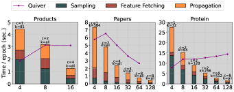
Figure 4: Performance results for our Graph Replication algorithm with GraphSAGE and compared with Quiver. For each GPU count, we break down the running time into 1) time spent sampling minibatches, 2) time spent in the all-to-allv call to gather necessary feature vectors, and 3) time spent on forward and backward propagation. In addition, for each GPU count, $c$ is the replication factor for the feature matrix, and $k$ is the number of minibatches sampled in a single bulk.

Quiver experiences a slowdown on all datasets going from $4$ to $8$ GPUs. This is likely attributable to cross-node communication, as each node on Perlmutter has $4$ GPUs. Thus, the first bar in each plot measures performance within one node, where all communication passes over high-bandwidth NVLink interconnects. Once we run experiments with $8$ GPUs and beyond, communication must pass over the lower-bandwidth cross-node Slingshot NICs.

Past $8$ GPUs, Quiver only scales on Papers, and does not scale at all on Products or Protein. This is likely because both Protein and Products are denser graphs, with an average degree of $241$ and $53$ compared to Papers ($29$). As a consequence, many features need to be communicated in the feature-fetching step, and Quiver does not effectively optimize this communication. This communication volume also increases as $p$ increases, causing Quiver to spend more time communicating and not scaling with $p$. Our pipeline is able to outperform to Quiver on large GPU counts since our feature fetching step scales with our replication factor $c$, along with our optimizations to sampling.

On low GPU counts, e.g. $4$ GPUs, we do not necessarily outperform Quiver particularly on Products and Protein. The advantages of our feature fetching approach come to fruition on larger GPU counts, as we do not have enough aggregate memory on lower GPU counts to replicate the feature matrix. In addition, our sampling optimizations are intended to amortize the cost of sampling over many minibatches. With only $4$ GPUs, we do not have enough memory to sample enough minibatches in bulk on Products and Protein to fully take advantage of our optimization. Note that in Figure 4, Products and Protein have a $k$ value smaller than their total minibatch count on $4$ GPUs. However, as we add more GPUs and aggregate memory, we are able to sample all minibatches in bulk for both Products and Protein. We are able to fully take advantage of our sampling operations at this point. For Papers, we are able to make sampling a small fraction of the total overall runtime on $4$ GPUs (only 10% of the total time is spent on sampling). Papers has a high-vertex count and a low-density. Thus, Papers has many minibatches to sample from, and each minibatch takes less space on device than a minibatch from Prodcuts or Protein. For this reason, we are able to sample a large number of batches in bulk on Papers with few GPUs, yielding good performance by our sampling optimization even on only $4$ GPUs.

8.1.2 Scaling Analysis

In Figure 4, we see good scaling on all datasets. We have an 88% parallel efficiency on Products, a 47% parallel efficiency on Papers, and a 61% parallel efficiency on Protein. Our sampling step scales nearly linearly with a $15.8\times$ speedup going from $4$ GPUs to $64$ GPUs on both Papers and Protein. This is because our sampling step in the Graph Replication algorithm involves no communication, and all minibatches in the $k$ to be sampled are partitioned across GPUs. Thus, the work per process goes does linearly, as evidenced by the linear scaling in sampling time. Our feature fetching time only decreases when we increase $c$. On Papers and Protein, our feature fetching time has a $5.5\times$ speedup in feature fetching time when increasing $c$ by $8\times$ Papers, and a $4.5\times$ speedup when increasing $c$ by $8\times$ on Protein. Our propagation time scales linearly as the number of minibatches trained per GPU goes down linearly with GPU count.

8.2 Graph Partitioned Algorithm

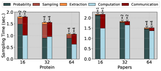
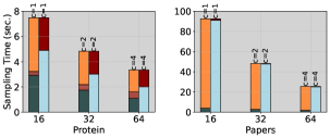
Figure 5: Scaling results for our Graph Partitioned algorithm. The first row of plots shows GraphSAGE timings, and the second row of plots shows LADIES timings. These plots only break down the time taken to sample minibatches, and breaks it down into the three steps outlined in Figures 3(a),3(b). We also break down the overall times into the time spent on communication and the time spent on computation. These times sample all minibatches in a single bulk sampling. For each GPU count, $c$ is the replication factor for all matrices. These times also sample all minibatches in a single bulk sampling over all possible minibatches.

8.2.1 GraphSAGE Performance Analysis

Figure 5 shows the performance breakdown of our framework for our large datasets across process counts. We do not show results on Products as it is small enough to fit on device for most GPUs. We measure sampling time, and show the time taken for each of the three steps in our sampling step (generating probability distributions, sampling from distributions, extracting adjacency matrices). We also show time taken by both computation and communication. For each process count, we plot the most performant replication factor.

Across all datasets, we see scaling up to $p=64$ GPUs. Protein sees $1.75\times$ speedup from $p=16$ to $p=64$, and Papers sees $1.43\times$ from $p=64$. This scaling behavior is consistent with the analysis in Section 5.2.1. Note that in Figure 5, a majority of time is spent on probability computation, which is a sparsity-aware 1.5D SpGEMM. We discuss the scaling results by analyzing communication and computation for the 1.5D SpGEMM separately.

Our analysis in Section 5.2.1 shows that the communication time primarily consists of $T_{rowdata}$ for sending row data and $T_{allreduce}$ for the final all-reduce call. The former scales with $c$, while the latter scales with $p/c$. Since $p>c$, significantly more time is spent communicating row data. For Protein, at least $3\times$ more time is spent on communication than reduction across all process counts in Figure 5. Since sending row data is the bottleneck in communication, communication overall scales when $c$ increases. For a fixed $p$, increasing $c$ dramatically speeds up the SpGEMM. $c$ cannot increase due to memory constraints, communication does not scale. This finding is consistent with prior work as well Buluç & Gilbert (2008). Buluç and Gilbert show that 1D SpGEMM algorithms are unscalable, where time increases with $p$. When $c$ is fixed but $p$ increases, the behavior is identical to that of 1D SpGEMM algorithms. Computation, on the other hand, largely scales with $p$. Both sampling and extraction are computation steps, and these are embarrassingly parallel across $p$.

8.2.2 LADIES Performance Analysis

For our LADIES results in Figure 5, we also see scaling across all datasets. Here, the time is dominated by the computation necessary for column extraction. This is logical, as column extraction multiplies more matrices than those in the probability computation or row extraction. In Equation 4.2.4, we see that column extraction multiplies a set of $\mathbf{A}_{R}\mathbf{Q}_{C}$ matrices. In theory this can be done in a single SpGEMM. In practice, however, this single SpGEMM is split into several smaller SpGEMMs to conserve memory, as $\mathbf{Q}_{C}$ contains many empty rows and cannot be stored efficiently in CSR format, which is necessary for SpGEMM.

9 Conclusion

In this work, we show that (1) a matrix-based approach to sample minibatches in bulk, and (2) a simple all-to-allv call with enough replication can outperform existing distributed GNN training systems. In the future, we hope to support additional sampling algorithms in our pipeline (e.g. graph-wise sampling). We also hope to investigate other types of communication-avoiding algorithms (e.g. 2D, 3D algorithms) when the graph must be partitioned.

References

- Azad et al. (2018) Azad, A., Pavlopoulos, G. A., Ouzounis, C. A., Kyrpides, N. C., and Buluç, A. HipMCL: a high-performance parallel implementation of the Markov clustering algorithm for large-scale networks. Nucleic Acids Research, 46(6):e33–e33, 01 2018. doi: 10.1093/nar/gkx1313. URL https://doi.org/10.1093/nar/gkx1313.
- Ballard et al. (2013) Ballard, G., Buluç, A., Demmel, J., Grigori, L., Lipshitz, B., Schwartz, O., and Toledo, S. Communication optimal parallel multiplication of sparse random matrices. pp. 222–231, 2013.
- Buluç & Gilbert (2011) Buluç, A. and Gilbert, J. R. The Combinatorial BLAS: Design, implementation, and applications. The International Journal of High Performance Computing Applications, 25(4):496–509, 2011.
- Buluç & Gilbert (2008) Buluç, A. and Gilbert, J. R. Challenges and advances in parallel sparse matrix-matrix multiplication. In The 37th International Conference on Parallel Processing (ICPP’08), pp. 503–510, Portland, Oregon, USA, September 2008. doi: 10.1109/ICPP.2008.45. URL http://eecs.berkeley.edu/~aydin/Buluc-ParallelMatMat.pdf.
- Cai et al. (2023) Cai, Z., Zhou, Q., Yan, X., Zheng, D., Song, X., Zheng, C., Cheng, J., and Karypis, G. Dsp: Efficient gnn training with multiple gpus. PPoPP ’23, pp. 392–404, 2023.
- Cao et al. (2023) Cao, K., Deng, R., Wu, S., Huang, E. W., Subbian, K., and Leskovec, J. Communication-free distributed gnn training with vertex cut, 2023.
- Chen et al. (2018) Chen, J., Ma, T., and Xiao, C. Fastgcn: fast learning with graph convolutional networks via importance sampling. arXiv preprint arXiv:1801.10247, 2018.
- Chiang et al. (2019) Chiang, W.-L., Liu, X., Si, S., Bengio, S., and Hsieh, C.-J. Cluster-gcn: An efficient algorithm for training deep and large graph convolutional networks. In Proceedings of the ACM SIGKDD International Conference on Knowledge Discovery and Data Mining (KDD), 2019.
- Corporation (2023) Corporation, N. NCCL: Optimized primitives for collective multi-gpu communication. https://github.com/NVIDIA/nccl, 2023.
- Fey & Lenssen (2019) Fey, M. and Lenssen, J. E. Fast graph representation learning with PyTorch Geometric. In ICLR Workshop on Representation Learning on Graphs and Manifolds, 2019.
- Gandhi & Iyer (2021) Gandhi, S. and Iyer, A. P. P3: Distributed deep graph learning at scale. In 15th USENIX Symposium on Operating Systems Design and Implementation (OSDI 21), pp. 551–568. USENIX Association, July 2021. ISBN 978-1-939133-22-9. URL https://www.usenix.org/conference/osdi21/presentation/gandhi.
- Gholami et al. (2018) Gholami, A., Azad, A., Jin, P., Keutzer, K., and Buluç, A. Integrated model, batch, and domain parallelism in training neural networks. In SPAA’18: 30th ACM Symposium on Parallelism in Algorithms and Architectures, 2018.
- Hamilton et al. (2017) Hamilton, W., Ying, Z., and Leskovec, J. Inductive representation learning on large graphs. In Guyon, I., Luxburg, U. V., Bengio, S., Wallach, H., Fergus, R., Vishwanathan, S., and Garnett, R. (eds.), Advances in Neural Information Processing Systems 30, pp. 1024–1034. Curran Associates, Inc., 2017. URL http://papers.nips.cc/paper/6703-inductive-representation-learning-on-large-graphs.pdf.
- Hu et al. (2020) Hu, W., Fey, M., Zitnik, M., Dong, Y., Ren, H., Liu, B., Catasta, M., and Leskovec, J. Open graph benchmark: Datasets for machine learning on graphs. arXiv preprint arXiv:2005.00687, 2020.
- Hübschle-Schneider & Sanders (2022) Hübschle-Schneider, L. and Sanders, P. Parallel weighted random sampling. volume 48, pp. 1–40. ACM, 2022.
- Jangda et al. (2021) Jangda, A., Polisetty, S., Guha, A., and Serafini, M. Accelerating graph sampling for graph machine learning using gpus. In EuroSys ’21: Proceedings of the Sixteenth European Conference on Computer Systems, pp. 311–326. ACM, 2021.
- Jia et al. (2020) Jia, Z., Lin, S., Gao, M., Zaharia, M., and Aiken, A. Improving the accuracy, scalability, and performance of graph neural networks with ROC. In Proceedings of Machine Learning and Systems (MLSys), pp. 187–198. 2020.
- Jiao et al. (2023) Jiao, X., Li, W., Wu, X., Hu, W., Li, M., Bian, J., Dai, S., Luo, X., Hu, M., Huang, Z., Feng, D., Yang, J., Feng, S., Xiong, H., Yu, D., Li, S., He, J., Ma, Y., and Liu, L. Pglbox: Multi-gpu graph learning framework for web-scale recommendation. In Proceedings of the 29th ACM SIGKDD Conference on Knowledge Discovery and Data Mining, KDD ’23, pp. 4262–4272, 2023.
- Kaler et al. (2023) Kaler, T., Iliopoulos, A., Murzynowski, P., Schardl, T., Leiserson, C. E., and Chen, J. Communication-efficient graph neural networks with probabilistic neighborhood expansion analysis and caching. In Proceedings of Machine Learning and Systems, 2023.
- Karypis & Kumar (1998) Karypis, G. and Kumar, V. A fast and high quality multilevel scheme for partitioning irregular graphs. In SIAM Journal of Scientific Computing, pp. 359–392. SIAM, 1998.
- Koanantakool et al. (2016) Koanantakool, P., Azad, A., Buluç, A., Morozov, D., Oh, S.-Y., Oliker, L., and Yelick, K. Communication-avoiding parallel sparse-dense matrix-matrix multiplication. In Proceedings of the IPDPS, 2016.
- Ma et al. (2019) Ma, L., Yang, Z., Miao, Y., Xue, J., Wu, M., Zhou, L., and Dai, Y. NeuGraph: Parallel deep neural network computation on large graphs. In USENIX Annual Technical Conference (USENIX ATC 19), pp. 443–458, Renton, WA, 2019. USENIX Association. ISBN 978-1-939133-03-8.
- (23) Nagasaka, Y., Nukada, A., and Matsuoka, S. Adaptive multi-level blocking optimization for sparse matrix vector multiplication on gpu. Procedia Comput. Sci., 80(C):131–142. ISSN 1877-0509. doi: 10.1016/j.procs.2016.05.304. URL https://doi.org/10.1016/j.procs.2016.05.304.
- Olver & Townsend (2013) Olver, S. and Townsend, A. Fast inverse transform sampling in one and two dimensions. arXiv preprint arXiv:1307.1223, 2013.
- Pandey et al. (2020) Pandey, S., Li, L., Hoisie, A., Li, X., and Liu, H. C-saw: A framework for graph sampling and random walk on gpus. In SC20: International Conference for High Performance Computing, Networking, Storage and Analysis, pp. 1–14. IEEE, 2020.
- Paszke et al. (2019) Paszke, A., Gross, S., Massa, F., Lerer, A., Bradbury, J., Chanan, G., Killeen, T., Lin, Z., Gimelshein, N., Antiga, L., et al. PyTorch: An imperative style, high-performance deep learning library. In Advances in Neural Information Processing Systems, pp. 8024–8035, 2019.
- Team (2023) Team, Q. Torch-quiver: Pytorch library for fast and easy distributed graph learning. https://github.com/quiver-team/torch-quiver, 2023.
- Tripathy et al. (2020) Tripathy, A., Yelick, K., and Buluç, A. Reducing communication in graph neural network training. In SC20: International Conference for High Performance Computing, Networking, Storage and Analysis, pp. 1–14. IEEE, 2020.
- Wan et al. (2022a) Wan, C., Li, Y., Li, A., Kim, N. S., and Lin, Y. BNS-GCN: Efficient full-graph training of graph convolutional networks with partition-parallelism and random boundary node sampling. Proceedings of Machine Learning and Systems, 4:673–693, 2022a.
- Wan et al. (2022b) Wan, C., Li, Y., Wolfe, C. R., Kyrillidis, A., Kim, N. S., and Lin, Y. PipeGCN: Efficient full-graph training of graph convolutional networks with pipelined feature communication. In International Conference on Learning Representations, 2022b. URL https://openreview.net/forum?id=kSwqMH0zn1F.
- Wu et al. (2020) Wu, Z., Pan, S., Chen, F., Long, G., Zhang, C., and Philip, S. Y. A comprehensive survey on graph neural networks. IEEE transactions on neural networks and learning systems, 32(1):4–24, 2020.
- Yang et al. (2022a) Yang, C., Buluç, A., and Owens, J. Graphblast: A high-performance linear algebra-based graph framework on the gpu. ACM Transactions on Mathematical Software, 48(1):1–51, 2022a.
- Yang et al. (2022b) Yang, D., Liu, J., Qi, J., and Lai, J. Wholegraph: A fast graph neural network training framework with multi-gpu distributed shared memory architecture. In Proceedings of the International Conference on High Performance Computing, Networking, Storage and Analysis, SC ’22, 2022b.
- Yang et al. (2022c) Yang, J., Tang, D., Song, X., Wang, L., Yin, Q., Chen, R., Yu, W., and Zhou, J. Gnnlab: A factored system for sample-based gnn training over gpus. In Proceedings of the Seventeenth European Conference on Computer Systems, EuroSys ’22, pp. 417–434, 2022c.
- Yang et al. (2019) Yang, K., Zhang, M., Chen, K., Ma, X., Bai, Y., and Jiang, Y. Knightking: A fast distributed graph random walk engine. 2019.
- Zeng et al. (2020) Zeng, H., Zhou, H., Srivastava, A., Kannan, R., and Prasanna, V. Graphsaint: Graph sampling based inductive learning method. In Proceedings of the International Conference on Learning Representations (ICLR), 2020.
- Zheng et al. (2020) Zheng, D., Ma, C., Wang, M., Zhou, J., Su, Q., Song, X., Gan, Q., Zhang, Z., and Karypis, G. Distdgl: distributed graph neural network training for billion-scale graphs. In 2020 IEEE/ACM 10th Workshop on Irregular Applications: Architectures and Algorithms (IA3), pp. 36–44. IEEE, 2020.
- Zhu et al. (2019) Zhu, R., Zhao, K., Yang, H., Lin, W., Zhou, C., Ai, B., Li, Y., and Zhou, J. AliGraph: a comprehensive graph neural network platform. Proceedings of the VLDB Endowment, 12(12):2094–2105, 2019.
- Zou et al. (2019) Zou, D., Hu, Z., Wang, Y., Jiang, S., Sun, Y., and Gu, Q. Layer-dependent importance sampling for training deep and large graph convolutional networks. In Proceedings of Neural Information Processing Systems (NeurIPS), 2019.