Global existence versus finite time blowup dichotomy for the dispersion managed NLS

Abstract.

We consider the Gabitov-Turitsyn equation or the dispersion managed nonlinear Schrödinger equation of a power-type nonlinearity

$$i\partial_{t}u+{d_{\mathrm{av}}}\partial_{x}^{2}u+\int_{0}^{1}e^{-ir\partial_{x}^{2}}\big{(}|e^{ir\partial_{x}^{2}}u|^{p-1}e^{ir\partial_{x}^{2}}u\big{)}dr=0$$

and prove the global existence versus finite time blowup dichotomy for the mass-supercritical cases, that is, $p>9$.

1. Introduction

In this paper, we consider the Cauchy problem for the dispersion managed nonlinear Schrödinger equation (NLS)

$$\begin{cases}\ \displaystyle{i\partial_{t}u+{d_{\mathrm{av}}}\partial_{x}^{2}u+\int_{0}^{1}e^{-ir\partial_{x}^{2}}\big{(}|e^{ir\partial_{x}^{2}}u|^{p-1}e^{ir\partial_{x}^{2}}u\big{)}dr=0,}\\[2.15277pt] \ u(0,\cdot)=u_{0}\end{cases}$$ (1.1)

where $u=u(t,x):I\times\mathbb{R}\to\mathbb{C}$ for an interval $I$, $p>1$, ${d_{\mathrm{av}}}\in{\mathbb{R}}$, and $e^{ir\partial_{x}^{2}}$ is the linear propagator.

The model (1.1) arises from the study of NLS with a periodically varying dispersion coefficient

$$i\partial_{t}u+d(t)\partial_{x}^{2}u+|u|^{p-1}u=0.$$ (1.2)

This equation describes the propagation of signals through glass-fiber cables with alternating sections of strongly positive and strongly negative dispersion, the so-called strong dispersion management. Here, $t$ corresponds to the distance along the fiber and $x$ denotes the (retarded) time. Hence, $d(t)$ is not varying in time but represents a dispersion varying along the optical cable. Specifically, the local dispersion $d(t)$ is given by

$$d(t)={d_{\mathrm{av}}}+\varepsilon^{-1}d_{0}(t/\varepsilon)$$

where ${d_{\mathrm{av}}}$ is the average component, $d_{0}$ is its mean zero part over one period and $\varepsilon$ is a small parameter. The technique of dispersion management was introduced in [23] and proved to be incredibly successful in producing stable, soliton-like pulses. See the reviews [27, 28] and the references cited in [19] for a discussion of the dispersion management technique. It is by now well-known that equation (1.2) with strong dispersion management can be averaged over one period to yield an effective equation, see [9, 10]. In particular, if $d_{0}$ is the $2$-periodic function with $d_{0}(t)=1$ on $[0,1)$ and $d_{0}(t)=-1$ on $[1,2)$, then the change of variables and the averaging process yield the equation of the form (1.1), called the Gabitov-Turitsyn equation. This averaging process is verified in [4, 30].

For the Cauchy problem (1.1), it is shown to be locally well-posed in $H^{1}(\mathbb{R})$ for all $p>1$ when ${d_{\mathrm{av}}}\neq 0$ ; $1<p\leq 5$ when ${d_{\mathrm{av}}}=0$, see [3]. Furthermore, its solution preserves the mass and the energy, that is, for all $t$,

$$M[u(t)]=M[u_{0}]\quad\mbox{and}\quad E[u(t)]=E[u_{0}],$$

where the mass and energy are defined by

$$M[f]:=\|f\|_{L^{2}}^{2}\quad\mbox{and}\quad E[f]:=\frac{{d_{\mathrm{av}}}}{2}\|\partial_{x}f\|^{2}_{L^{2}}-\frac{1}{p+1}\int_{0}^{1}\|e^{ir\partial_{x}^{2}}f\|^{p+1}_{L^{p+1}}dr.$$

When ${d_{\mathrm{av}}}$ is negative, by the conservation laws, solutions are extended to be global in time for all $p>1$. In the singular case ${d_{\mathrm{av}}}=0$ and $1<p\leq 5$, the mass conservation law guarantees global existence in $L^{2}({\mathbb{R}})$, and then by the persistence of regularity, $H^{1}({\mathbb{R}})$-solutions exist globally in time. On the other hand, if the average dispersion ${d_{\mathrm{av}}}$ is positive, the model admits a much richer dynamics in that it corresponds to the focusing case in the classical NLS. In particular, the model has soliton-like pulses made of ground states. See [2, 3, 12, 30] for the existence and their properties. They are relatively well explored even in the case ${d_{\mathrm{av}}}=0$, see [7, 17, 18, 19, 22, 26].

In this paper, we focus on the situation where finite time blowup may occur. We consider the positive average dispersion case ${d_{\mathrm{av}}}>0$. For numerical simplification, we reduce to the case ${d_{\mathrm{av}}}=1$, but we also assume that $p\geq 9$. In spite of lack of scaling invariance, we assert that the equation is mass-critical (resp., mass-supercritical) if $p=9$ (resp., $p>9$). Note that given a solution $u(t,x)$ to (1.1), $u_{\lambda}(t,x)=\lambda^{\frac{4}{p-1}}u(\lambda^{2}t,\lambda x)$ solves the equation with a different $r$-averaged nonlinearity,

$$i\partial_{t}u_{\lambda}+\partial_{x}^{2}u_{\lambda}+\int_{0}^{1/\lambda^{2}}e^{-ir\partial_{x}^{2}}\big{(}|e^{ir\partial_{x}^{2}}u_{\lambda}|^{p-1}e^{ir\partial_{x}^{2}}u_{\lambda}\big{)}dr=0$$

with the initial data $u_{0;\lambda}(x)=\lambda^{\frac{4}{p-1}}u_{0}(\lambda x)$ for any $\lambda>0$, and that $M[u_{0;\lambda}]=M[u_{0}]$ if and only if $p=9$. Another evidence is that the equation is globally well-posed in $H^{1}({\mathbb{R}})$ when $1<p<9$, see [3].

The main purpose of our work is to justify that the case $p>9$ can be classified as mass-supercritical for the dispersion managed NLS (1.1) by showing that it admits finite time blowups. Even more than that, we provide a precise description on the global versus blowup dichotomy for the equation (1.1). We note that this is the first result establishing the dichotomy for the dispersion managed NLS. Indeed, even existence of finite time blowup solutions was not known before.

We recall that for the classical power-type NLS, the global versus blowup dichotomy is stated in terms of a specific extremizer for an appropriate Gagliardo-Nirenberg inequality and that a non-scattering solitary wave is given by the extremizer, see [14, 29]. Then, global solutions in the dichotomy are shown to scatter, so the dynamics below the extremizer are completely characterized, see [5, 6, 15, 21]. An interesting question is to obtain the same scattering versus blowup dichotomy picture for the dispersion managed NLS. In this direction, our main result gives an affirmative answer for the first step to the so-called Kenig-Merle program.

For the dispersion managed NLS, at first glance, one may guess from the definition of the energy functional that the following local-in-time Gagliardo-Nirenberg-Strichartz estimate

$$\int_{0}^{1}\|e^{ir\partial_{x}^{2}}f\|_{L^{p+1}}^{p+1}dr\leq C\|f\|_{L^{2}}^{\frac{p+7}{2}}\|\partial_{x}f\|_{L^{2}}^{\frac{p-5}{2}}$$ (1.3)

would be a candidate substituting the Gagliardo-Nirenberg inequality for the classical NLS. However, due to the presence of the finite interval $[0,1]$, the inequality (1.3) is no longer invariant under scaling. It turns out that the sharp constant for (1.3) is given by that of the global-in-time Gagliardo-Nirenberg-Strichartz estimate

$$\|e^{ir\partial_{x}^{2}}f\|_{L_{r,x}^{p+1}}^{p+1}\leq C\|f\|_{L^{2}}^{\frac{p+7}{2}}\|\partial_{x}f\|_{L^{2}}^{\frac{p-5}{2}},$$ (1.4)

where

$$\|u\|_{L^{q}_{r,x}}:=\|u\|_{L_{r}^{q}({\mathbb{R}},L_{x}^{q}({\mathbb{R}}))}=\left(\int_{\mathbb{R}}\int_{\mathbb{R}}|u(r,x)|^{q}dxdr\right)^{\frac{1}{q}},\quad 1\leq q<\infty.$$

Theorem 1.1 (Critical element for the inequality (1.4)).

We define the Weinstein functional associated with the inequality (1.4) by

$$W_{p}(f)=\frac{\|e^{ir\partial_{x}^{2}}f\|_{L_{r,x}^{p+1}}^{p+1}}{\|f\|_{L^{2}}^{\frac{p+7}{2}}\|\partial_{x}f\|_{L^{2}}^{\frac{p-5}{2}}}.$$

Then, for $p\geq 9$, the variational problem

$$\mathcal{C}_{p}=\sup_{f\in H^{1}({\mathbb{R}})}W_{p}(f)$$

admits a maximizer $Q\in H^{1}({\mathbb{R}})$ which solves the Euler-Lagrange equation

$$-\partial_{x}^{2}Q+Q-\int_{\mathbb{R}}e^{-ir\partial_{x}^{2}}\big{(}|e^{ir\partial_{x}^{2}}Q|^{p-1}e^{ir\partial_{x}^{2}}Q\big{)}dr=0.$$ (1.5)

Moreover, the sharp constant $\mathcal{C}_{p}$ for the global inequality (1.4) is equal to that for the local inequality (1.3).

Remarks 1.2.

• Unlike the classical NLS, we do not know uniqueness (up to symmetries) of the critical element for the Weinstein functional. However, by construction, the important norm quantities can be expressed only in terms of $\mathcal{C}_{p}$ and $p$, and they are independent of a possibly non-unique profile $Q$. Precisely, we have $\|Q\|_{L^{2}}^{2}=\big{[}\frac{2(p+1)(p-5)}{(p+7)^{2}\mathcal{C}_{p}}\big{]}^{\frac{2}{p-1}}\cdot\big{(}\frac{p+7}{p-5}\big{)}^{\frac{1}{2}}$, $\|\partial_{x}Q\|^{2}_{L^{2}}=\frac{p-5}{p+7}\|Q\|^{2}_{L^{2}}$ and $\|e^{ir\partial_{x}^{2}}Q\|_{L_{r,x}^{p+1}}^{p+1}=\frac{2(p+1)}{p+7}\|Q\|_{L^{2}}^{2}$, see Lemma 4.5.

• Some precise upper and lower bounds for the sharp constant $\mathcal{C}_{p}$ are given in Lemma 4.1.

• As a consequence of Theorem 1.1, it is easy to see that there is no maximizer for the local-in-time Gagliardo-Nirenberg-Strichartz estimate (1.3), see Remark 4.6.

We note that $u(t,x)=Q(x)e^{it}$ is a solitary wave for a rather theoretical scaling-invariant limit equation

$$i\partial_{t}u+\partial_{x}^{2}u+\int_{\mathbb{R}}e^{-ir\partial_{x}^{2}}\big{(}|e^{ir\partial_{x}^{2}}u|^{p-1}e^{ir\partial_{x}^{2}}u\big{)}dr=0,$$

and it preserves the energy over ${\mathbb{R}}$ defined by

$$E_{\infty}[f]:=\frac{1}{2}\|\partial_{x}f\|_{L^{2}}^{2}-\frac{1}{p+1}\|e^{ir\partial_{x}^{2}}f\|_{L_{r,x}^{p+1}}^{p+1}$$

and the same mass.

Using the extremizer in the previous theorem, we state our main result on the global existence versus finite time blowup dichotomy.

Theorem 1.3 (Global versus blowup criteria).

Let $p>9$. Suppose that

$$E[u_{0}]M[u_{0}]^{\alpha}<E_{\infty}[Q]M[Q]^{\alpha},$$ (1.6)

where $\alpha=\frac{p+7}{p-9}$ and $Q$ is given in Theorem 1.1, and let $u(t)$ be the $H^{1}({\mathbb{R}})$-solution to the equation (1.1) with initial data $u_{0}$ whose the maximal forward time interval of existence is $[0,T_{\max})$.

• If

  $$\|\partial_{x}u_{0}\|_{L^{2}}\|u_{0}\|_{L^{2}}^{\alpha}<\|\partial_{x}Q\|_{L^{2}}\|Q\|_{L^{2}}^{\alpha},$$ (1.7)

  then

  $$\|\partial_{x}u(t)\|_{L^{2}}\|u(t)\|_{L^{2}}^{\alpha}<\|\partial_{x}Q\|_{L^{2}}\|Q\|_{L^{2}}^{\alpha}\quad\textup{for all }t\in[0,T_{\max})$$ (1.8)

  and $u(t)$ exists globally in time, i.e., $T_{\max}=\infty$.

• If

  $$\|\partial_{x}u_{0}\|_{L^{2}}\|u_{0}\|_{L^{2}}^{\alpha}>\|\partial_{x}Q\|_{L^{2}}\|Q\|_{L^{2}}^{\alpha}$$ (1.9)

  then

  $$\|\partial_{x}u(t)\|_{L^{2}}\|u(t)\|_{L^{2}}^{\alpha}>\|\partial_{x}Q\|_{L^{2}}\|Q\|_{L^{2}}^{\alpha}\quad\textup{for all }t\in[0,T_{\max}).$$ (1.10)

  Furthermore, if $|\cdot|u_{0}\in L^{2}({\mathbb{R}})$, then $T_{\max}<\infty$ so that the solution blows up in finite time.

Remark 1.4.

It follows from Remark 1.2 (i) that the key quantities $\|\partial_{x}Q\|_{L^{2}}\|Q\|_{L^{2}}^{\alpha}$ and $E_{\infty}[Q]M[Q]^{\alpha}$ also can be written using $\mathcal{C}_{p}$ and $p$, precisely,

$$\|\partial_{x}Q\|_{L^{2}}\|Q\|_{L^{2}}^{\alpha}=\left[\frac{2(p+1)}{(p-5)\mathcal{C}_{p}}\right]^{\frac{2}{p-9}}$$ (1.11)

and

$$E_{\infty}[Q]M[Q]^{\alpha}=\frac{p-9}{2(p-5)}\|\partial_{x}Q\|_{L^{2}}^{2}\|Q\|_{L^{2}}^{2\alpha}=\frac{p-9}{2(p-5)}\left[\frac{2(p+1)}{(p-5)\mathcal{C}_{p}}\right]^{\frac{4}{p-9}}.$$ (1.12)

Remark 1.5 (Negative energy implies blowup).

The subset of $H^{1}(\mathbb{R})$ satisfying (1.6) can be characterized as in Figure 1. From the picture, one can see that Theorem 1.3 (ii) includes that negative energy solutions having finite variance blow up in finite time, which is analogous to the classical result of Glassey [11].

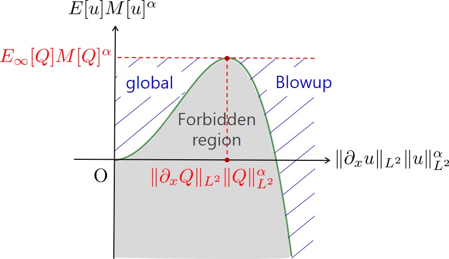
Figure 1. Global existence versus blowup dichotomy

Remark 1.6 (Mass-critical case, $p=9$).

In the mass-critical case, global existence is shown in [3, Theorem 1.6 (ii)] when $\|u_{0}\|_{L^{2}}$ is small enough. We have a precise sufficient condition for global existence in terms of the extremizer in Theorem 1.1. More precisely, if $\|u_{0}\|_{L^{2}}<\|Q\|_{L^{2}}$, then the solution exists global in time. Indeed, it follows from the conservation laws, Theorem 1.1 and the identities in Remark 1.2 (i) that

$$E[u_{0}] =E[u(t)]=\frac{1}{2}\|\partial_{x}u(t)\|_{L^{2}}^{2}-\frac{1}{10}\int_{0}^{1}\|e^{ir\partial_{x}^{2}}u(t)\|_{L^{10}}^{10}dr$$

$$\geq\frac{1}{2}\|\partial_{x}u(t)\|_{L^{2}}^{2}-\frac{1}{10}\frac{\|e^{ir\partial_{x}^{2}}Q\|_{L_{r,x}^{10}}^{10}}{\|Q\|_{L^{2}}^{8}\|\partial_{x}Q\|_{L^{2}}^{2}}\|u(t)\|_{L^{2}}^{8}\|\partial_{x}u(t)\|_{L^{2}}^{2}$$

$$=\frac{1}{2}\|\partial_{x}u(t)\|_{L^{2}}^{2}\left(1-\frac{\|u_{0}\|^{8}_{L^{2}}}{\|Q\|_{L^{2}}^{8}}\right).$$

Therefore, if $\|u_{0}\|_{L^{2}}<\|Q\|_{L^{2}}$, then $u(t)$ exists globally in time. On the other hand, if $\|u_{0}\|_{L^{2}}>\|Q\|_{L^{2}}$ and if, in addition, $E[u_{0}]<0$ and $\|xu_{0}\|_{L^{2}}<\infty$, then it follows from Proposition 3.1 and a density argument that the solution blows up in finite time.

One of the main contributions of this paper is to provide an explicit calculation for the second derivative of the variance for the dispersion managed NLS, see Section 3. Similar calculations have potential applications to various dynamical problems of the model in the form of (localized) virial/Morawetz identities, which will be postponed to future work. Indeed, proving virial/Morawetz identities in general can be done by elementary integration by parts with a weight function. However, unlike the power-type case, the dispersion managed NLS includes the linear propagator $e^{ir\partial_{x}^{2}}$ in the nonlinearity, so more careful analysis is required to deal with to commute the weight function with the propagator and vice versa, see (3.2). More importantly, while doing integration by parts, additional time boundary terms appear at $r=0,1$, see (3.3) and (3.6). An important remark is that if we repeat the same calculation with the nonlinearity

$$\int_{r_{0}}^{r_{1}}e^{-ir\partial_{x}^{2}}(|e^{ir\partial_{x}^{2}}u|^{p-1}e^{ir\partial_{x}^{2}}u)dr,\quad r_{0}<r_{1},$$

then a good negative sign term is obtained at the right endpoint $r_{1}$, while a bad positive sign term is obtained at the left endpoint $r_{0}$. However, in the physically relevant case, $r_{0}$ is taken to be zero and it removes the bad sign term. This is a key observation in our proof.

The paper is organized as follows: In Section 2, we review the local theory in $H^{1}({\mathbb{R}})$ for the Cauchy problem (1.1) and present the local theory in $H^{3,3}({\mathbb{R}})$ in order to ensure finite variance which is key for the existence of finite time blowup solutions. In Section 3, we prove the virial estimate by modifying the method of Glassey [11]. The proof of Theorem 1.1 which is a central analytic tool in this paper is presented in Section 4. Finally, in Section 5, we establish the global existence versus blowup dichotomy, Theorem 1.3.

$\mathbf{Notation.}$ We write $f\lesssim g$ if a finite constant $C>0$ exists such that $f\leq Cg$. For $k\in{\mathbb{N}}$, we denote by $H^{k,k}({\mathbb{R}})$ the weighted Sobolev space equipped with the norm

$$\|f\|_{H^{k,k}}:=\left\{\|f\|_{L^{2}}^{2}+\|\partial_{x}^{k}f\|_{L^{2}}^{2}+\big{\|}x^{k}f\big{\|}_{L^{2}}^{2}\right\}^{\frac{1}{2}}.$$

2. Preliminary local theory

In this section, we discuss the local theory in both $H^{1}({\mathbb{R}})$ and $H^{3,3}({\mathbb{R}})$ for (1.1). First, we recall the local existence result in $H^{1}(\mathbb{R})$ from [3].

Theorem 2.1 (Theorem 1.3 in [3]).

Given initial data $u_{0}\in H^{1}({\mathbb{R}})$, there exists a unique maximal solution $u\in C([0,T_{\max});H^{1}({\mathbb{R}}))$ of (1.1). The solution $u(t)$ is maximal in the sense that if $T_{\max}<\infty$ then $\|u(t)\|_{H^{1}}\to\infty$ as $t\uparrow T_{\max}$. Moreover, for all $t\in[0,T_{\max})$, it conserves the mass

$$M[u(t)]=M[u_{0}]$$

and the energy

$$\quad E[u(t)]=E[u_{0}].$$

We complete the local well-posedness in $H^{1}({\mathbb{R}})$ by proving that solutions depend continuously on initial data. It can be proved by a standard argument, but for the reader’s convenience, we give its proof.

Lemma 2.2 (Continuity of the data-to-solution map).

Let $u\in C([0,T_{\textup{max}});H^{1}(\mathbb{R}))$ be the maximal solution of (1.1) with initial data $u_{0}\in H^{1}(\mathbb{R})$. Then, for any $T\in(0,T_{\textup{max}})$, there exist small $\delta>0$ and large $K\geq 1$ such that if $\|\tilde{u}_{0}-u_{0}\|_{H^{1}}\leq\delta$, then the equation (1.1) has a unique solution $\tilde{u}\in C([0,T];H^{1}(\mathbb{R}))$ with initial data $\tilde{u}_{0}\in H^{1}(\mathbb{R})$ and

$$\|\tilde{u}-u\|_{C([0,T];H^{1})}\leq K\|\tilde{u}_{0}-u_{0}\|_{H^{1}}.$$

Proof.

It follows from Proposition 3.5 in [3] that there is $T_{1}>0$, depending only on $p$ and $\|u_{0}\|_{H^{1}}$, such that both $u(t)$ and $\tilde{u}(t)$ exist in $H^{1}({\mathbb{R}})$ and $\|u(t)\|_{H^{1}},\|\tilde{u}(t)\|_{H^{1}}\leq 2\|u_{0}\|_{H^{1}}$ for all $t\in(0,T_{1}]$, whenever $\tilde{u}_{0}$ is sufficiently close to $u_{0}$ in $H^{1}({\mathbb{R}})$.

Applying the estimates used in the proof of Theorem 1.3 in [3], one can show that

$$\|(u-\tilde{u})(t)\|_{H^{1}}\leq\|u_{0}-\tilde{u}_{0}\|_{H^{1}}+C\int_{0}^{t}\Big{(}\|u(s)\|_{H^{1}}^{p-1}+\|\tilde{u}(s)\|_{H^{1}}^{p-1}\Big{)}\|(u-\tilde{u})(s)\|_{H^{1}}ds$$

for all $t$. Hence, it follows from Grönwall’s inequality that

$$\|(\tilde{u}-u)(t)\|_{H^{1}} \leq\|\tilde{u}_{0}-u_{0}\|_{H^{1}}\exp\bigg{(}C\int_{0}^{t}\|\tilde{u}(s)\|_{H^{1}}^{p-1}+\|u(s)\|_{H^{1}}^{p-1}ds\bigg{)}$$

$$\leq\|\tilde{u}_{0}-u_{0}\|_{H^{1}}\exp\bigg{(}\widetilde{C}\int_{0}^{t}\|u(s)\|_{H^{1}}^{p-1}+\|(\tilde{u}-u)(s)\|_{H^{1}}^{p-1}ds\bigg{)}.$$ (2.1)

Therefore, by taking

$$K=2\exp\bigg{(}\widetilde{C}\int_{0}^{T}\|u(s)\|_{H^{1}}^{p-1}ds\bigg{)}\geq 2,$$

we can choose $T_{*}\in(0,T_{1}]$ such that

$$\sup_{t\in[0,T_{*}]}\|(\tilde{u}-u)(t)\|_{H^{1}}\leq\frac{3K}{4}\|\tilde{u}_{0}-u_{0}\|_{H^{1}}\leq\frac{3K\delta}{4}.$$ (2.2)

To cover the interval $[0,T]$, we substitute (2.2) in (2.1), then we have

$$\sup_{t\in[0,T_{*}]}\|(\tilde{u}-u)(t)\|_{H^{1}}\leq\frac{K}{2}\exp\bigg{(}\widetilde{C}T\frac{(3K\delta)^{p-1}}{4^{p-1}}\bigg{)}\|\tilde{u}_{0}-u_{0}\|_{H^{1}}.$$

Taking $\delta>0$ small, (2.2) is improved as

$$\sup_{t\in[0,T_{*}]}\|(\tilde{u}-u)(t)\|_{H^{1}}\leq\frac{2K}{3}\|\tilde{u}_{0}-u_{0}\|_{H^{1}}.$$

This means that one can extend the existence time for $\tilde{u}(t)$ from $T_{*}$ to $T$, keeping (2.2). ∎

Next, we prove the local existence in $H^{3,3}({\mathbb{R}})$ employing the following estimate.

Lemma 2.3.

We have

$$\big{\|}(x-2it\partial_{x})^{3}f\big{\|}_{L^{2}}\lesssim(1+|t|)^{3}\|f\|_{H^{3,3}}$$

for all $f\in H^{3,3}({\mathbb{R}})$ and $t\in{\mathbb{R}}$.

Proof.

Since

$$(x-2it\partial_{x})^{3}=x^{3}-6itx^{2}\partial_{x}-6itx-12t^{2}x\partial_{x}^{2}-12t^{2}\partial_{x}+8it^{3}\partial_{x}^{3},$$

it suffices to show that

$$\big{\|}x^{2}\partial_{x}f\big{\|}_{L^{2}}+\big{\|}x\partial_{x}^{2}f\big{\|}_{L^{2}}\lesssim\|f\|_{H^{3,3}}$$ (2.3)

for all $f\in C_{c}^{\infty}(\mathbb{R})$, by density. Taking the integration by parts, we have

$$\|x^{2}\partial_{x}f\|_{L^{2}}^{2}+\|x\partial_{x}^{2}f\|_{L^{2}}^{2}$$

$$=\int_{\mathbb{R}}x^{4}\partial_{x}f\overline{\partial_{x}f}+x^{2}\partial_{x}^{2}f\overline{\partial_{x}^{2}f}\,dx$$

$$=-\int_{\mathbb{R}}\big{(}4x^{3}\partial_{x}f+x^{4}\partial_{x}^{2}f)\overline{f}\,dx-\int_{\mathbb{R}}(2x\partial_{x}^{2}f+x^{2}\partial_{x}^{3}f)\overline{\partial_{x}f}\,dx$$

$$=-\int_{\mathbb{R}}\big{(}4x^{3}\partial_{x}f+x^{4}\partial_{x}^{2}f)\overline{f}\,dx-\int_{\mathbb{R}}x^{2}\partial_{x}^{3}f\overline{\partial_{x}f}\,dx+\int_{\mathbb{R}}(2\partial_{x}^{2}f+2x\partial_{x}^{3}f)\overline{f}\,dx.$$

Thus, using the Cauchy-Schwarz inequality, we obtain

$$\|x^{2}\partial_{x}f\|_{L^{2}}^{2}+\|x\partial_{x}^{2}f\|_{L^{2}}^{2} \leq 4\|x^{3}f\|_{L^{2}}\|\partial_{x}f\|_{L^{2}}+\|x^{3}f\|_{L^{2}}\|x\partial_{x}^{2}f\|_{L^{2}}+\|\partial_{x}^{3}f\|_{L^{2}}\|x^{2}\partial_{x}f\|_{L^{2}}$$

$$\quad+2\|\partial_{x}^{2}f\|_{L^{2}}\|f\|_{L^{2}}+2\|\partial_{x}^{3}f\|_{L^{2}}\|xf\|_{L^{2}}$$

$$\leq 8\|f\|_{H^{3,3}}^{2}+\|f\|_{H^{3,3}}\|x\partial_{x}^{2}f\|_{L^{2}}+\|f\|_{H^{3,3}}\|x^{2}\partial_{x}f\|_{L^{2}}$$

$$\leq 9\|f\|_{H^{3,3}}^{2}+\frac{1}{2}\|x^{2}\partial_{x}f\|_{L^{2}}^{2}+\frac{1}{2}\|x\partial_{x}^{2}f\|_{L^{2}}^{2}$$

which yields (2.3). ∎

Lemma 2.4 (Local existence in $H^{3,3}(\mathbb{R})$).

Given initial data $u_{0}\in H^{3,3}(\mathbb{R})$, there exists $\widetilde{T}_{\max}\in(0,\infty]$ and a unique maximal solution $u\in C([0,\widetilde{T}_{\textup{max}});H^{3,3}(\mathbb{R}))$ of (1.1). The solution $u(t)$ is maximal in the sense that if $\widetilde{T}_{\max}<\infty$, then $\|u(t)\|_{H^{3,3}}\to\infty$ as $t\uparrow\widetilde{T}_{\max}$.

Proof.

For each $T,a>0$, let

$$B_{T,a}=\{u\in C([0,T];H^{3,3}({\mathbb{R}}))\;:\;\|u\|_{L^{\infty}([0,T],H^{3,3})}\leq a\}$$

be equipped with the norm $\|u\|_{L^{\infty}([0,T];H^{3,3})}$. Let $u_{0}\in H^{3,3}({\mathbb{R}})$ be fixed and define the map $\Gamma_{u_{0}}$ on $B_{T,a}$ by

$$\Gamma_{u_{0}}(u)=e^{it\partial_{x}^{2}}u_{0}+i\int_{0}^{t}\int_{0}^{1}e^{i(t-s)\partial_{x}^{2}}e^{-ir\partial_{x}^{2}}\big{(}|e^{ir\partial_{x}^{2}}u|^{p-1}e^{ir\partial_{x}^{2}}u\big{)}(s)drds.$$

Using the identity

$$xe^{ir\partial_{x}}=e^{ir\partial_{x}}(x-2ir\partial_{x}),$$

the unitarity of $e^{it\partial_{x}^{2}}$ on $L^{2}({\mathbb{R}})$, and Lemma 2.3, we have

$$\|\Gamma_{u_{0}}(u)\|_{H^{3,3}}\lesssim(1+t)^{3}\|u_{0}\|_{H^{3,3}}+\int_{0}^{t}\int_{0}^{1}(1+|t-s-r|)^{3}\big{\|}\big{(}|e^{ir\partial_{x}^{2}}u|^{p-1}e^{ir\partial_{x}^{2}}u\big{)}(s)\big{\|}_{H^{3,3}}drds.$$

For the nonlinear term, use the fact

$$x^{3}|e^{ir\partial_{x}^{2}}u|^{p-1}e^{ir\partial_{x}^{2}}u=|e^{ir\partial_{x}^{2}}u|^{p-1}\Bigl{(}x^{3}e^{ir\partial_{x}^{2}}u\Bigr{)}=|e^{ir\partial_{x}^{2}}u|^{p-1}e^{ir\partial_{x}^{2}}(x-2ir\partial_{x})^{3}u,$$

Lemma 2.3, the Sobolev embedding $H^{1}({\mathbb{R}})\hookrightarrow L^{\infty}({\mathbb{R}})$, and the unitarity of $e^{ir\partial_{x}^{2}}$ on $H^{1}({\mathbb{R}})$, then we obtain

$$\big{\|}|e^{ir\partial_{x}^{2}}u|^{p-1}e^{ir\partial_{x}^{2}}u\big{\|}_{H^{3,3}}\lesssim\|u\|_{H^{1}}^{p-1}\|u\|_{H^{3,3}}$$

for all $r\in[0,1]$. Therefore, combining the two inequalities, we get

$$\|\Gamma_{u_{0}}(u)\|_{L^{\infty}([0,T];H^{3,3})}\lesssim(1+T)^{3}\left(\|u_{0}\|_{H^{3,3}}+\int_{0}^{T}\|u(s)\|_{H^{3,3}}^{p}ds\right).$$

Similarly, we have

$$\|\Gamma_{u_{0}}(u)-\Gamma_{u_{0}}(v)\|_{L^{\infty}([0,T];H^{3,3})}$$

$$\lesssim(1+T)^{3}\int_{0}^{T}\int_{0}^{1}\big{\|}\big{(}|e^{ir\partial_{x}^{2}}u|^{p-1}e^{ir\partial_{x}^{2}}u-|e^{ir\partial_{x}^{2}}v|^{p-1}e^{ir\partial_{x}^{2}}v\big{)}(s)\big{\|}_{H^{3,3}}drds$$

$$\lesssim(1+T)^{3}\int_{0}^{T}\big{(}\|u(s)\|^{p-1}_{H^{3,3}}+\|v(s)\|^{p-1}_{H^{3,3}}\big{)}\|(u-v)(s)\|_{H^{3,3}}ds$$

Thus, for all $u,v\in B_{T,a}$, there exists $C>0$, depending on $p$, such that we have

$$\|\Gamma_{u_{0}}(u)\|_{C([0,T];H^{3,3})}\leq C(1+T)^{3}a+C(1+T)^{3}Ta^{p}$$

and

$$d(\Gamma_{u_{0}}(u),\Gamma_{u_{0}}(v))\leq C(1+T)^{3}Ta^{p-1}d(u,v).$$

Taking $a\geq\|u_{0}\|_{H^{3,3}}$, it follows that $\Gamma_{u_{0}}$ is a contraction from $B_{T,a}$ to itself for a sufficiently small $T>0$, depending on $\|u_{0}\|_{H^{3,3}}$. Therefore, by the Banach fixed point theorem, there exists a unique solution $u$ in $B_{T,a}$. By a standard argument, we extend the solution $u$ to the maximal interval $[0,\widetilde{T}_{\max})$ so that $u\in C([0,\widetilde{T}_{\max});H^{3,3}({\mathbb{R}}))$ with either $\widetilde{T}_{\max}=\infty$ or $\lim_{t\uparrow\widetilde{T}_{\max}}\|u(t)\|_{H^{3,3}}=\infty$. ∎

We end this section by proving the $H^{3,3}$ regularity of $H^{1}$ solution.

Lemma 2.5 (Persistence of regularity).

Suppose that $u\in C([0,\widetilde{T}_{\textup{max}});H^{3,3}(\mathbb{R}))$ is a solution of (1.1) with initial data $u_{0}\in H^{3,3}(\mathbb{R})$ and the maximal existence time $\widetilde{T}_{\textup{max}}$ is finite, that is, $\|u(t)\|_{H^{3,3}}\to\infty$ as $t\uparrow\widetilde{T}_{\textup{max}}$. Then, $\|u(t)\|_{H^{1}}\to\infty$ as $t\uparrow\widetilde{T}_{\textup{max}}$. As a consequence, $\widetilde{T}_{\textup{max}}=T_{\textup{max}}$, where $T_{\textup{max}}$ is the maximal existence time in Theorem 2.1.

Proof.

Suppose to the contrary that $\|u\|_{L^{\infty}([0,\widetilde{T}_{\textup{max}});H^{1})}<\infty$. Arguing similarly as in the proof of Lemma 2.4, one can show that

$$\|u(t)\|_{H^{3,3}}\lesssim(1+|t|)^{3}\|u_{0}\|_{H^{3,3}}+\int_{0}^{t}(1+|t-s|)^{3}\|u(s)\|_{H^{1}}^{p-1}\|u(s)\|_{H^{3,3}}ds.$$

Hence, Grönwall’s inequality yields the bound

$$\|u(t)\|_{H^{3,3}}\lesssim(1+|t|)^{3}\|u_{0}\|_{H^{3,3}}\exp\bigg{(}\int_{0}^{t}(1+|t-s|)^{3}\|u(s)\|_{H^{1}}^{p-1}ds\bigg{)},$$

which implies that as long as $u(t)$ is finite in $H^{1}(\mathbb{R})$, it is finite in $H^{3,3}({\mathbb{R}})$. Taking the limit as $t\uparrow\widetilde{T}_{\textup{max}}$ deduces a contradiction. ∎

3. Virial estimate

In this section, we modify the standard virial identity of Glassey [11] dealing with the variance. In order to ensure finite variance and use the virial argument, we require the initial data $u_{0}$ to be in $H^{3,3}({\mathbb{R}})$.

Proposition 3.1.

Let $u\in C([0,\widetilde{T}_{\max});H^{3,3}({\mathbb{R}}))$ be the maximal solution of (1.1) with initial data $u_{0}\in H^{3,3}({\mathbb{R}})$. If the variance is defined by

$$\mathcal{V}(t)=\int_{\mathbb{R}}x^{2}|u(t,x)|^{2}dx,$$

then

$$\mathcal{V}(t)\leq\mathcal{V}(0)+\mathcal{V}_{1}^{\prime}(0)t+\int_{0}^{t}\int_{0}^{s}\Phi(\tau)d\tau ds$$

for all $0\leq t<\widetilde{T}_{\max}$, where

$$\mathcal{V}_{1}^{\prime}(t)=4\textup{Im}\int_{\mathbb{R}}x\partial_{x}u(t,x)\overline{u(t,x)}dx$$

and

$$\Phi(t)=16E[u_{0}]-\frac{4(p-9)}{p+1}\int_{0}^{1}\int_{\mathbb{R}}|e^{ir\partial_{x}^{2}}u(t,x)|^{p+1}dxdr.$$ (3.1)

Proof.

Let $u\in C([0,\widetilde{T}_{\max});H^{3,3}({\mathbb{R}}))$ be the maximal solution of (1.1). We first calculate the first derivative of $\mathcal{V}$ as follows. Using equation in (1.1), we write

$$\mathcal{V}^{\prime}(t) =2\textup{Re}\int_{\mathbb{R}}x^{2}\overline{u(t,x)}\partial_{t}u(t,x)dx$$

$$=-2\textup{Im}\int_{\mathbb{R}}x^{2}\overline{u(t,x)}\partial_{x}^{2}u(t,x)dx$$

$$\quad-2\textup{Im}\int_{\mathbb{R}}\int_{0}^{1}\overline{(e^{ir\partial_{x}^{2}}x^{2}u)(t,x)}\big{(}|e^{ir\partial_{x}^{2}}u|^{p-1}e^{ir\partial_{x}^{2}}u\big{)}(t,x)drdx$$

$$=:\mathcal{V}_{1}^{\prime}(t)+\mathcal{V}_{2}^{\prime}(t).$$

By the integration by parts,

$$\mathcal{V}_{1}^{\prime}(t)=4\textup{Im}\int_{\mathbb{R}}x\partial_{x}u(t,x)\overline{u(t,x)}dx.$$

Here, the boundary terms disappear since $\partial_{x}u\in H^{1}({\mathbb{R}})$ and

$$\|x^{2}u\|_{H^{1}}\lesssim\|xu\|_{L^{2}}+\|x^{2}u\|_{L^{2}}+\|x^{2}\partial_{x}u\|_{L^{2}}\lesssim\|u\|_{H^{3,3}}$$

where (2.3) is used.

For $\mathcal{V}_{2}^{\prime}(t)$, note the identities

$$e^{ir\partial_{x}^{2}}x=(x+2ir\partial_{x})e^{ir\partial_{x}^{2}}\quad\textup{and}\quad\partial_{x}^{2}e^{ir\partial_{x}^{2}}=-i\partial_{r}e^{ir\partial_{x}^{2}}$$ (3.2)

to get

$$e^{ir\partial_{x}^{2}}x^{2} =(x+2ir\partial_{x})^{2}e^{ir\partial_{x}^{2}}$$

$$=(x^{2}+4irx\partial_{x}+2ir-4r^{2}\partial_{x}^{2})e^{ir\partial_{x}^{2}}$$

$$=\big{(}x^{2}+i(4rx\partial_{x}+2r+4r^{2}\partial_{r})\big{)}e^{ir\partial_{x}^{2}}.$$

Hence, using the integration by parts again, we obtain

$$\mathcal{V}_{2}^{\prime}(t) =-2\textup{Re}\int_{\mathbb{R}}\int_{0}^{1}\overline{\big{(}(4rx\partial_{x}+2r+4r^{2}\partial_{r})e^{ir\partial_{x}^{2}}u\big{)}(t,x)}(|e^{ir\partial_{x}^{2}}u|^{p-1}e^{ir\partial_{x}^{2}}u)(t,x)drdx$$ (3.3)

$$=-\frac{8}{p+1}\int_{\mathbb{R}}\int_{0}^{1}x\partial_{x}\big{(}|e^{ir\partial_{x}^{2}}u(t,x)|^{p+1}\big{)}rdrdx-4\int_{\mathbb{R}}\int_{0}^{1}|e^{ir\partial_{x}^{2}}u(t,x)|^{p+1}rdrdx$$

$$\quad-\frac{8}{p+1}\int_{\mathbb{R}}\int_{0}^{1}\partial_{r}\big{(}|e^{ir\partial_{x}^{2}}u(t,x)|^{p+1}\big{)}r^{2}drdx$$

$$=-\frac{8}{p+1}\int_{0}^{1}\left[x|e^{ir\partial_{x}^{2}}u(t,x)|^{p+1}\Big{|}_{x=-\infty}^{x=\infty}-\int_{\mathbb{R}}|e^{ir\partial_{x}^{2}}u(t,x)|^{p+1}dx\right]rdr$$

$$\quad-\frac{4(p-3)}{p+1}\int_{\mathbb{R}}\int_{0}^{1}|e^{ir\partial_{x}^{2}}u(t,x)|^{p+1}rdrdx-\frac{8}{p+1}\int_{\mathbb{R}}|e^{ir\partial_{x}^{2}}u(t,x)|^{p+1}r^{2}\Big{|}_{r=0}^{r=1}dx.$$

Now we note that $x|e^{ir\partial_{x}^{2}}u(t,x)|^{p+1}$ is in $H^{1}({\mathbb{R}})$ for each $r\in[0,1]$. Indeed, by the Sobolev inequality, (3.2), and a similar argument as when obtaining (2.3), we see that

$$\|x|e^{ir\partial_{x}^{2}}u|^{p+1}\|_{L^{2}} \leq\|e^{ir\partial_{x}^{2}}u\|^{p}_{L^{\infty}}\|xe^{ir\partial_{x}^{2}}u\|_{L^{2}}$$

$$\leq\|e^{ir\partial_{x}^{2}}u\|^{p}_{H^{1}}\|(x-2ir\partial_{x})u\|_{L^{2}}\lesssim(1+r)\|u\|^{p}_{H^{1}}\|u\|_{H^{1,1}}$$

and

$$\|x|e^{ir\partial_{x}^{2}}u|^{p}\partial_{x}(e^{ir\partial_{x}^{2}}u)\|_{L^{2}} \leq\|e^{ir\partial_{x}^{2}}u\|^{p}_{L^{\infty}}\|xe^{ir\partial_{x}^{2}}(\partial_{x}u)\|_{L^{2}}$$

$$\leq\|e^{ir\partial_{x}^{2}}u\|^{p}_{H^{1}}\|(x-2ir\partial_{x})(\partial_{x}u)\|_{L^{2}}\lesssim(1+r)\|u\|^{p}_{H^{1}}\|u\|_{H^{2,2}}$$

and therefore $x|e^{ir\partial_{x}^{2}}u(t,x)|^{p+1}\in H^{1}({\mathbb{R}})$ since $u\in H^{3,3}({\mathbb{R}})$. Thus, the boundary terms $x|e^{ir\partial_{x}^{2}}u(t,x)|^{p+1}\Big{|}_{-\infty}^{\infty}$ vanish and so

$$\mathcal{V}_{2}^{\prime}(t)=-\frac{4(p-5)}{p+1}\int_{\mathbb{R}}\int_{0}^{1}|e^{ir\partial_{x}^{2}}u(t,x)|^{p+1}rdrdx-\frac{8}{p+1}\int_{\mathbb{R}}|e^{i\partial_{x}^{2}}u(t,x)|^{p+1}dx<0.$$ (3.4)

Therefore, using the fundamental theorem of calculus, we have

$$\mathcal{V}(t)\leq\mathcal{V}(0)+\int_{0}^{t}\mathcal{V}_{1}^{\prime}(\tau)d\tau$$ (3.5)

for all $t>0$ since $\mathcal{V}^{\prime}(t)\leq\mathcal{V}_{1}^{\prime}(t)$ by (3.4).

Differentiating $\mathcal{V}_{1}^{\prime}(t)=4\textup{Im}\int_{\mathbb{R}}x\partial_{x}u(t,x)\overline{u(t,x)}dx$ and then using the integration by parts, we obtain

$$\mathcal{V}_{1}^{\prime\prime}(t) =4\textup{Im}\int_{\mathbb{R}}x\Bigl{(}\partial_{x}\partial_{t}u(t,x)\Bigr{)}\overline{u(t,x)}dx+4\textup{Im}\int_{\mathbb{R}}x\partial_{x}u(t,x)\overline{\partial_{t}u(t,x)}dx$$

$$=-4\textup{Im}\int_{\mathbb{R}}\partial_{t}u(t,x)\overline{u(t,x)}dx+8\textup{Im}\int_{\mathbb{R}}x\partial_{x}u(t,x)\overline{\partial_{t}u(t,x)}dx.$$

Then, using equation in (1.1) and the integration by parts, again, we get

$$\mathcal{V}_{1}^{\prime\prime}(t) =-4\textup{Re}\int_{\mathbb{R}}\left\{\partial_{x}^{2}u+\int_{0}^{1}e^{-ir\partial_{x}^{2}}(|e^{ir\partial_{x}^{2}}u|^{p-1}e^{ir\partial_{x}^{2}}u)dr\right\}(t,x)\overline{u(t,x)}dx$$

$$\quad-8\textup{Re}\int_{\mathbb{R}}x\left\{\partial_{x}^{2}u+\int_{0}^{1}e^{-ir\partial_{x}^{2}}(|e^{ir\partial_{x}^{2}}u|^{p-1}e^{ir\partial_{x}^{2}}u)dr\right\}(t,x)\overline{\partial_{x}u(t,x)}dx$$

$$=8\|\partial_{x}u(t,x)\|_{L^{2}}^{2}-4\int_{\mathbb{R}}\int_{0}^{1}|e^{ir\partial_{x}^{2}}u(t,x)|^{p+1}drdx$$

$$\quad-8\textup{Re}\int_{\mathbb{R}}\int_{0}^{1}(|e^{ir\partial_{x}^{2}}u|^{p-1}e^{ir\partial_{x}^{2}}u)(t,x)\overline{e^{ir\partial_{x}^{2}}(x\partial_{x}u)(t,x)}drdx.$$

On the other hand, it follows from the identities in (3.2) that

$$e^{ir\partial_{x}^{2}}x\partial_{x}=(x+2ir\partial_{x})e^{ir\partial_{x}^{2}}\partial_{x}=x\partial_{x}e^{ir\partial_{x}^{2}}+2r\partial_{r}e^{ir\partial_{x}^{2}}.$$

Hence, by a similar argument in (3.3), we have

$$-\textup{Re}\int_{\mathbb{R}}\int_{0}^{1}(|e^{ir\partial_{x}^{2}}u|^{p-1}e^{ir\partial_{x}^{2}}u)(t,x)\overline{e^{ir\partial_{x}^{2}}(x\partial_{x}u)(t,x)}drdx$$ (3.6)

$$=-\textup{Re}\int_{\mathbb{R}}\int_{0}^{1}(|e^{ir\partial_{x}^{2}}u|^{p-1}e^{ir\partial_{x}^{2}}u)(t,x)\overline{(x\partial_{x}e^{ir\partial_{x}^{2}}u+2r\partial_{r}e^{ir\partial_{x}^{2}}u)(t,x)}drdx$$

$$=-\frac{2}{p+1}\int_{\mathbb{R}}|e^{i\partial_{x}^{2}}u(t,x)|^{p+1}dx+\frac{3}{p+1}\int_{\mathbb{R}}\int_{0}^{1}|e^{ir\partial_{x}^{2}}u(t,x)|^{p+1}drdx$$

$$\leq\frac{3}{p+1}\int_{\mathbb{R}}\int_{0}^{1}|e^{ir\partial_{x}^{2}}u(t,x)|^{p+1}drdx.$$

Therefore, it follows from the energy conservation that

$$\mathcal{V}_{1}^{\prime\prime}(t) \leq 8\|\partial_{x}u(t)\|_{L^{2}}^{2}-\frac{4(p-5)}{p+1}\int_{0}^{1}\int_{\mathbb{R}}|e^{ir\partial_{x}^{2}}u(t,x)|^{p+1}dxdr$$

$$=16E[u_{0}]-\frac{4(p-9)}{p+1}\int_{0}^{1}\int_{\mathbb{R}}|e^{ir\partial_{x}^{2}}u(t,x)|^{p+1}dxdr=\Phi(t).$$

By the fundamental theorem of calculus again, for all $t>0$

$$\mathcal{V}_{1}^{\prime}(t)\leq\mathcal{V}_{1}^{\prime}(0)+\int_{0}^{t}\Phi(s)ds$$

and therefore by (3.5)

$$\mathcal{V}(t)\leq\mathcal{V}(0)+\mathcal{V}_{1}^{\prime}(0)t+\int_{0}^{t}\int_{0}^{s}\Phi(\tau)d\tau ds.$$

∎

4. Proof of Theorem 1.1

In this section, we consider the variational problem

$$\mathcal{C}_{p}=\sup_{f\in H^{1}({\mathbb{R}})}W_{p}(f)=\sup_{f\in H^{1}({\mathbb{R}})}\frac{\|e^{ir\partial_{x}^{2}}f\|_{L_{r,x}^{p+1}}^{p+1}}{\|f\|_{L^{2}}^{\frac{p+7}{2}}\|\partial_{x}f\|_{L^{2}}^{\frac{p-5}{2}}},$$

where $\|u\|_{L^{q}_{r,x}}:=\|u\|_{L_{r}^{q}({\mathbb{R}},L_{x}^{q}({\mathbb{R}}))}$ for $1\leq q<\infty$. The following lemma provides a rough estimate for the best constant $\mathcal{C}_{p}$, so the variational problem $\mathcal{C}_{p}$ is well-formulated.

Lemma 4.1 (Upper and lower bounds for $\mathcal{C}_{p}$).

$$\frac{2^{\frac{p-7}{4}}}{\pi^{\frac{p-1}{4}}(p+1)^{\frac{1}{2}}}B\left(\frac{1}{2},\frac{p-3}{4}\right)=\frac{2^{\frac{p-7}{4}}}{\pi^{\frac{p-3}{4}}(p+1)^{\frac{1}{2}}}\frac{\Gamma(\frac{p-3}{4})}{\Gamma(\frac{p-1}{4})}\leq\mathcal{C}_{p}\leq\frac{1}{2\sqrt{3}},$$

where $B$ is the beta function and $\Gamma$ is the gamma function. In particular, $\frac{1}{2\sqrt{5}\pi}\leq\mathcal{C}_{9}\leq\frac{1}{2\sqrt{3}}$.

Proof.

For every $f\in H^{1}({\mathbb{R}})$, we have

$$\|e^{ir\partial_{x}^{2}}f\|_{L_{r,x}^{p+1}}^{p+1} \leq\int_{\mathbb{R}}\|e^{ir\partial_{x}^{2}}f\|_{L^{\infty}}^{p-5}\|e^{ir\partial_{x}^{2}}f\|_{L^{6}}^{6}dr$$

$$\leq\|f\|_{L^{2}}^{\frac{p-5}{2}}\|\partial_{x}f\|_{L^{2}}^{\frac{p-5}{2}}\|e^{ir\partial_{x}^{2}}f\|_{L_{r,x}^{6}}^{6}.$$

Then, by the Strichartz estimate in one dimension

$$\|e^{ir\partial_{x}^{2}}f\|_{L_{r,x}^{6}}\leq\frac{1}{12^{1/12}}\|f\|_{L^{2}}$$

with the best constant $\frac{1}{12^{1/12}}$, see [8, 20], it follows that

$$\|e^{ir\partial_{x}^{2}}f\|_{L_{r,x}^{p+1}}^{p+1}\leq\frac{1}{\sqrt{12}}\|f\|_{L^{2}}^{\frac{p+7}{2}}\|\partial_{x}f\|_{L^{2}}^{\frac{p-5}{2}}.$$ (4.1)

For the lower bound, we employ the Gaussian test-function $\varphi(x)=e^{-\frac{1}{2}x^{2}}$. Note that $\|\varphi\|_{L^{2}}^{2}=\sqrt{\pi}$ and $\|\partial_{x}\varphi\|_{L^{2}}^{2}=\sqrt{\pi}/2$. Moreover, its free time evolution is given by

$$e^{ir\partial_{x}^{2}}\varphi(x)=\left(\frac{1}{1+2ir}\right)^{\frac{1}{2}}e^{-\frac{x^{2}}{2(1+2ir)}}$$

and therefore

$$\|e^{ir\partial_{x}^{2}}\varphi\|_{L^{p+1}}^{p+1}=\left(\frac{2\pi}{p+1}\right)^{\frac{1}{2}}\left(\frac{1}{1+4r^{2}}\right)^{\frac{p-1}{4}}$$

see, e.g., [2, 30]. Then we have

$$W_{p}(\varphi)=\frac{\|e^{ir\partial_{x}^{2}}\varphi\|_{L_{r,x}^{p+1}}^{p+1}}{\|\varphi\|_{L^{2}}^{\frac{p+7}{2}}\|\partial_{x}\varphi\|_{L^{2}}^{\frac{p-5}{2}}}=\frac{2^{\frac{p+1}{4}}}{\pi^{\frac{p-1}{4}}(p+1)^{\frac{1}{2}}}\int_{0}^{\infty}\left(\frac{1}{1+4r^{2}}\right)^{\frac{p-1}{4}}dr.$$

The integral is rewritten as the beta function that

$$\int_{0}^{\infty}\left(\frac{1}{1+4r^{2}}\right)^{\frac{p-1}{4}}dr=\frac{1}{2}\int_{0}^{\frac{\pi}{2}}\cos^{\frac{p-5}{2}}\theta d\theta=\frac{1}{4}B\left(\frac{1}{2},\frac{p-3}{4}\right)$$

where we used $B(x,y)=2\int_{0}^{\pi/2}(\sin\theta)^{2x-1}(\cos\theta)^{2y-1}d\theta$. Using the relation between the beta function and gamma function, we obtain the lower bound in the lemma. ∎

We prove the existence of a maximizer for the variational problem $\mathcal{C}_{p}$ and derive its Euler-Lagrange equation.

Proposition 4.2 (Existence of a maximizer for $\mathcal{C}_{p}$ ).

For $p\geq 9$, there exists a maximizer $g\in H^{1}({\mathbb{R}})$ for the variational problem $\mathcal{C}_{p}$ such that $\|g\|_{L^{2}}=\|\partial_{x}g\|_{L^{2}}=1$. Moreover, $g$ solves

$$\frac{p-5}{2}\partial_{x}^{2}g-\frac{p+7}{2}g+\frac{p+1}{\mathcal{C}_{p}}\int_{\mathbb{R}}e^{-ir\partial_{x}^{2}}\big{(}|e^{ir\partial_{x}^{2}}g|^{p-1}e^{ir\partial_{x}^{2}}g\big{)}dr=0.$$

To begin with, such a critical element can be constructed by a standard concentration-compactness argument of Lions [24, 25]. Among many different formulations, we particularly employ one in the form of the profile decomposition, see [13, Proposition 3.4] for instance.

Lemma 4.3 (Profile decomposition).

Let $\{f_{n}\}_{n\in{\mathbb{N}}}$ be a uniformly bounded sequence in $H^{1}({\mathbb{R}})$ such that $\displaystyle\limsup_{n\to\infty}\|f_{n}\|_{L^{2}}\neq 0$. Then, up to a subsequence, there exists a nonzero $g\in H^{1}({\mathbb{R}})$ and sequences of time shifts $\{r_{n}\}_{n\in{\mathbb{N}}}$ and space shifts $\{x_{n}\}_{n\in{\mathbb{N}}}$ such that

$$e^{ir_{n}\partial_{x}^{2}}f_{n}(\cdot+x_{n})\rightharpoonup g\quad\mbox{in}\quad H^{1}({\mathbb{R}}).$$

We define the sequence $R_{n}$ of remainders by

$$f_{n}=e^{-ir_{n}\partial_{x}^{2}}g(\cdot-x_{n})+R_{n}.$$

Then, the above decomposition satisfies the asymptotic Pythagorean rule,

$$\|f_{n}\|_{L^{2}}^{2}=\|g\|_{L^{2}}^{2}+\|R_{n}\|_{L^{2}}^{2}+o_{n}(1),$$ (4.2)

$$\|\partial_{x}f_{n}\|_{L^{2}}^{2}=\|\partial_{x}g\|_{L^{2}}^{2}+\|\partial_{x}R_{n}\|_{L^{2}}^{2}+o_{n}(1)$$ (4.3)

and

$$\|e^{ir\partial_{x}^{2}}f_{n}\|_{L_{r,x}^{p+1}}^{p+1}=\|e^{ir\partial_{x}^{2}}g\|_{L_{r,x}^{p+1}}^{p+1}+\|e^{ir\partial_{x}^{2}}R_{n}\|_{L_{r,x}^{p+1}}^{p+1}+o_{n}(1).$$ (4.4)

We need to show (4.4) only, as all the other can be obtained from [13, Propositions 3.4] and its proof. We modify the method by Brézis-Lieb [1] to prove (4.4).

Proof.

Replacing $e^{ir_{n}\partial_{x}^{2}}f_{n}(\cdot+x_{n})$ by $f_{n}$, we may assume that $x_{n}=0$ and $r_{n}=0$ so that $f_{n}\rightharpoonup g$ in $H^{1}({\mathbb{R}})$ and $f_{n}=g+R_{n}$, where $R_{n}=e^{ir_{n}\partial_{x}^{2}}R_{n}(\cdot+x_{n})$ . Then, there exists a subsequence of $\{f_{n}\}_{n\in{\mathbb{N}}}$, but still denoted by $\{f_{n}\}_{n\in{\mathbb{N}}}$, such that $f_{n}\to g$ a.e. in ${\mathbb{R}}$. It suffices to prove that

$$\lim_{n\to\infty}\int_{\mathbb{R}}\int_{{\mathbb{R}}}\left||e^{ir\partial_{x}^{2}}f_{n}|^{p+1}-|e^{ir\partial_{x}^{2}}R_{n}|^{p+1}-|e^{ir\partial_{x}^{2}}g|^{p+1}\right|dxdr=0.$$ (4.5)

Let $\varepsilon>0$ be fixed. Observe that by Young’s inequality

$$||a+b|^{p+1}-|a|^{p+1}| =\left|\int_{0}^{1}\frac{d}{ds}(|a+sb|^{p+1})ds\right|$$ (4.6)

$$\leq({p+1})\int_{0}^{1}|a+sb|^{p}|b|ds$$

$$\leq C\varepsilon|a|^{p+1}+C(\varepsilon)|b|^{p+1}$$

for all $a,b\in{\mathbb{C}}$. Applying (4.6) with $a=e^{ir\partial_{x}^{2}}R_{n}$ and $b=e^{ir\partial_{x}^{2}}g$, we see that

$$\left||e^{ir\partial_{x}^{2}}f_{n}|^{p+1}-|e^{ir\partial_{x}^{2}}R_{n}|^{p+1}-|e^{ir\partial_{x}^{2}}g|^{p+1}\right|$$ (4.7)

$$\leq\left||e^{ir\partial_{x}^{2}}f_{n}|^{p+1}-|e^{ir\partial_{x}^{2}}R_{n}|^{p+1}\right|+|e^{ir\partial_{x}^{2}}g|^{p+1}$$

$$\leq C\varepsilon|e^{ir\partial_{x}^{2}}R_{n}|^{p+1}+C(\varepsilon)|e^{ir\partial_{x}^{2}}g|^{p+1}+|e^{ir\partial_{x}^{2}}g|^{p+1}.$$

Let

$$F_{n}^{\varepsilon}(r,x):=\left[\left||e^{ir\partial_{x}^{2}}f_{n}(x)|^{p+1}-|e^{ir\partial_{x}^{2}}R_{n}(x)|^{p+1}-|e^{ir\partial_{x}^{2}}g(x)|^{p+1}\right|-C\varepsilon|e^{ir\partial_{x}^{2}}R_{n}(x)|^{p+1}\right]_{+},$$

where $a_{+}=\max(a,0)$ for any $a\in{\mathbb{R}}$. For now, we fix $r\in{\mathbb{R}}$. Then, up to a subsequence, $F_{n}^{\varepsilon}(r,\cdot)\to 0$ for a.e. $x$ since $\{e^{ir\partial_{x}^{2}}f_{n}\}_{n\in{\mathbb{N}}}$ is also uniformly bounded in $H^{1}({\mathbb{R}})$ and $f_{n}\to g$ for a.e. $x$. Moreover, by (4.7) and the Sobolev embedding,

$$F_{n}^{\varepsilon}(r,\cdot)\leq C(\varepsilon)|e^{ir\partial_{x}^{2}}g|^{p+1}+|e^{ir\partial_{x}^{2}}g|^{p+1}\in L_{x}^{1}({\mathbb{R}}).$$

Thus, by the dominated convergence theorem, $\int_{\mathbb{R}}F_{n}^{\varepsilon}(r,x)\,dx\to 0$. Next, the sequence of functions of $r$ is bounded as

$$\int_{\mathbb{R}}F_{n}^{\varepsilon}(r,x)\,dx\leq\int_{\mathbb{R}}\left(C(\varepsilon)|e^{ir\partial_{x}^{2}}g|^{p+1}+|e^{ir\partial_{x}^{2}}g|^{p+1}\right)dx\in L_{r}^{1}({\mathbb{R}})$$

by (4.1). Using the dominated convergence theorem again, we have $\int_{\mathbb{R}}\int_{\mathbb{R}}F_{n}^{\varepsilon}(r,x)\,dxdr\to 0$. Hence, we have

$$\limsup_{n\to\infty}\int_{\mathbb{R}}\int_{\mathbb{R}}\left||e^{ir\partial_{x}^{2}}f_{n}|^{p+1}-|e^{ir\partial_{x}^{2}}R_{n}|^{p+1}-|e^{ir\partial_{x}^{2}}g|^{p+1}\right|dxdr$$

$$\leq\limsup_{n\to\infty}\left(\int_{\mathbb{R}}\int_{\mathbb{R}}F_{n}^{\varepsilon}(r)dxdr+C\varepsilon\int_{\mathbb{R}}\int_{\mathbb{R}}|e^{ir\partial_{x}^{2}}R_{n}|^{p+1}dxdr\right)\leq C\varepsilon$$

by $\{R_{n}\}_{n\in{\mathbb{N}}}$ begin uniformly bounded in $H^{1}({\mathbb{R}})$ and (4.1). Since $\varepsilon>0$ is arbitrary, this proves (4.5). ∎

We use the following elementary inequality to eliminate the splitting scenario in the concentration-compactness argument.

Lemma 4.4 (Algebraic inequality [16]).

For any $a_{1},a_{2},b_{1},b_{2}>0$ and $s>1$, if $\frac{a_{1}}{a_{2}^{s}}\geq\frac{b_{1}}{b_{2}^{s}}$, then

$$\frac{a_{1}}{a_{2}^{s}}\geq\frac{a_{1}+b_{1}}{(a_{2}+b_{2})^{s}}.$$

Further assume that $\delta\leq\frac{b_{2}}{a_{2}}\leq\frac{1}{\delta}$ for some $\delta>0$, then there exists $c=c(\delta)>1$ such that

$$\frac{a_{1}}{a_{2}^{s}}\geq c\frac{a_{1}+b_{1}}{(a_{2}+b_{2})^{s}}.$$

Now we are ready to give the

Proof of Proposition 4.2.

Let $\{f_{n}\}_{n\in{\mathbb{N}}}\subset H^{1}({\mathbb{R}})$ be a maximizing sequence for $\mathcal{C}_{p}$, i.e., $W_{p}(f_{n})\to\mathcal{C}_{p}$. Note that if define

$$f_{\lambda,\mu}(x)=\mu f(\lambda x)\quad\mbox{for any }\lambda,\mu>0,$$ (4.8)

then

$$\|f_{\lambda,\mu}\|_{L^{2}}^{2}=\mu^{2}\lambda^{-1}\|f\|^{2}_{L^{2}},\quad\|\partial_{x}f_{\lambda,\mu}\|^{2}_{L^{2}}=\mu^{2}\lambda\|\partial_{x}f\|^{2}_{L^{2}}$$ (4.9)

and

$$\|e^{ir\partial_{x}^{2}}f_{\lambda,\mu}\|_{L^{p+1}_{r,x}}^{p+1}=\mu^{p+1}\lambda^{-3}\|e^{ir\partial_{x}^{2}}f\|_{L^{p+1}_{r,x}}^{p+1}$$

and therefore $W_{\mathbb{R}}^{p}(f_{\lambda,\mu})=W_{\mathbb{R}}^{p}(f)$, that is, the functional $W_{{\mathbb{R}}}^{p}(f)$ is invariant under scaling and multiplication by a constant. Thus, we may assume that $\|f_{n}\|_{L^{2}}=\|f_{n}^{\prime}\|_{L^{2}}=1$ for each $n\in{\mathbb{N}}$.

According to Lemma 4.3, there is a subsequence of $\{f_{n}\}_{n\in{\mathbb{N}}}$, but still denoted by $\{f_{n}\}_{n\in{\mathbb{N}}}$, a nonzero profile $g\in H^{1}({\mathbb{R}})$, sequences of time shifts $\{r_{n}\}_{n\in{\mathbb{N}}}$ and space shifts $\{x_{n}\}_{n\in{\mathbb{N}}}$ such that

$$f_{n}=e^{-ir_{n}\partial_{x}^{2}}g(\cdot-x_{n})+R_{n}$$ (4.10)

satisfying (4.2)-(4.4). Note from (4.2) and (4.3) that $0<\|g\|_{L^{2}},\|\partial_{x}g\|_{L^{2}}\leq 1$. Moreover, by the space-time translation invariance of the quantities in the functional $W_{p}(f)$, we may assume that $r_{n}=0$ and $x_{n}=0$ for all $n$ in (4.10) so that

$$f_{n}=g+R_{n}.$$

We claim that $g$ is a maximizer with $\|g\|_{L^{2}}=\|\partial_{x}g\|_{L^{2}}=1$. To prove the claim, it suffices to show

$$\liminf_{n\to\infty}\|e^{ir\partial_{x}^{2}}R_{n}\|_{L^{p+1}_{r,x}}=0.$$ (4.11)

Indeed, it follows from (4.4) with (4.11) and $0<\|g\|_{L^{2}},\|\partial_{x}g\|_{L^{2}}\leq 1$ that

$$\mathcal{C}_{p} =\lim_{n\to\infty}W_{p}(f_{n})=\lim_{n\to\infty}\|e^{ir\partial_{x}^{2}}f_{n}\|_{L_{r,x}^{p+1}}^{p+1}=\|e^{ir\partial_{x}^{2}}g\|_{L_{r,x}^{p+1}}^{p+1}$$

$$\leq\frac{\|e^{ir\partial_{x}^{2}}g\|_{L_{r,x}^{p+1}}^{p+1}}{\|g\|_{L^{2}}^{\frac{p+7}{2}}\|\partial_{x}g\|_{L^{2}}^{\frac{p-5}{2}}}=W_{p}(g)\leq\mathcal{C}_{p}.$$

Therefore, we conclude that $W_{p}(g)=\mathcal{C}_{p}$ and $\|g\|_{L^{2}}=\|\partial_{x}g\|_{L^{2}}=1$. Now, for (4.11), suppose to the contrary that

$$\liminf_{n\to\infty}\|e^{ir\partial_{x}^{2}}R_{n}\|_{L^{p+1}_{r,x}}>0.$$

Then, it follows from (4.1), (4.2), and (4.3) that

$$0<\lim_{n\to\infty}\|R_{n}\|_{L^{2}}\leq 1,\quad 0<\lim_{n\to\infty}\|\partial_{x}R_{n}\|_{L^{2}}\leq 1.$$ (4.12)

Using (4.2)-(4.4), we can write

$$W_{p}(f_{n})=\frac{\|e^{ir\partial_{x}^{2}}g\|_{L_{r,x}^{p+1}}^{p+1}+\|e^{ir\partial_{x}^{2}}R_{n}\|_{L_{r,x}^{p+1}}^{p+1}}{\left(\|g\|_{L^{2}}^{2}+\|R_{n}\|_{L^{2}}^{2}\right)^{\frac{p+7}{4}}}+o_{n}(1).$$

We consider the following two cases,

$$\frac{\|e^{ir\partial_{x}^{2}}g\|_{L_{r,x}^{p+1}}^{p+1}}{\|g\|_{L^{2}}^{\frac{p+7}{2}}}\geq\liminf_{n\to\infty}\frac{\|e^{ir\partial_{x}^{2}}R_{n}\|_{L_{r,x}^{p+1}}^{p+1}}{\|R_{n}\|_{L^{2}}^{\frac{p+7}{2}}}\quad\mbox{and}\quad\frac{\|e^{ir\partial_{x}^{2}}g\|_{L_{r,x}^{p+1}}^{p+1}}{\|g\|_{L^{2}}^{\frac{p+7}{2}}}<\liminf_{n\to\infty}\frac{\|e^{ir\partial_{x}^{2}}R_{n}\|_{L_{r,x}^{p+1}}^{p+1}}{\|R_{n}\|_{L^{2}}^{\frac{p+7}{2}}}.$$

In the former case, by Lemma 4.4, we have

$$W_{p}(f_{n})\leq\frac{\|e^{ir\partial_{x}^{2}}g\|_{L_{r,x}^{p+1}}^{p+1}}{\|g\|_{L^{2}}^{\frac{p+7}{2}}}+o_{n}(1)$$

up to a subsequence. Then, since $0<\|\partial_{x}g\|_{L^{2}}\leq 1$, we obtain

$$\mathcal{C}_{p}=\lim_{n\to\infty}W_{p}(f_{n})\leq\frac{\|e^{ir\partial_{x}^{2}}g\|_{L_{r,x}^{p+1}}^{p+1}}{\|g\|_{L^{2}}^{\frac{p+7}{2}}}\leq\frac{\|e^{ir\partial_{x}^{2}}g\|_{L_{r,x}^{p+1}}^{p+1}}{\|g\|_{L^{2}}^{\frac{p+7}{2}}\|\partial_{x}g\|_{L^{2}}^{\frac{p-5}{2}}}=W_{p}(g)\leq\mathcal{C}_{p},$$

which implies $\|\partial_{x}g\|_{L^{2}}=1$. It follows from (4.3) and $\|\partial_{x}f_{n}\|_{L^{2}}=1$ that $\|\partial_{x}R_{n}\|_{L^{2}}\to 0$, which contradicts (4.12). In the latter case, let $\delta=\lim_{n\to\infty}\|R_{n}\|_{L^{2}}^{2}$ then $0<\delta\leq 1$ due to (4.12). By applying Lemma 4.4, there exists $c>1$, independent of $n$, such that

$$cW_{p}(f_{n})\leq\,\frac{\|e^{ir\partial_{x}^{2}}R_{n}\|_{L_{r,x}^{p+1}}^{p+1}}{\|R_{n}\|_{L^{2}}^{\frac{p+7}{2}}}+o_{n}(1)\leq W_{p}(R_{n})+o_{n}(1)$$

for sufficiently large $n$, where we used (4.12) in the second inequality. Thus, one sees that

$$\mathcal{C}_{p}=\lim_{n\to\infty}W_{p}(f_{n})<c\lim_{n\to\infty}W_{p}(f_{n})\leq\liminf_{n\to\infty}W_{p}(R_{n}),$$

which is a contradiction.

From the standard argument in the calculus of variations, the above maximizer $g\in H^{1}({\mathbb{R}})$ is a weak solution of the associated Euler-Lagrange equation

$$\left.\frac{d}{d\varepsilon}\right|_{\varepsilon=0}W_{p}(g+\varepsilon\eta)=0$$

for all $\eta\in C_{0}^{\infty}({\mathbb{R}})$. Considering that $\|g\|_{L^{2}}=1$ and $\|\partial_{x}g\|_{L^{2}}=1$, we have

$$\frac{p-5}{2}\partial_{x}^{2}g-\frac{p+7}{2}g+\frac{p+1}{\mathcal{C}_{p}}\int_{\mathbb{R}}e^{-ir\partial_{x}^{2}}\big{(}|e^{ir\partial_{x}^{2}}g|^{p-1}e^{ir\partial_{x}^{2}}g\big{)}dr=0.$$ (4.13)

Observe that every weak solution $f\in H^{1}({\mathbb{R}})$ of (4.13) is in $H^{3}({\mathbb{R}})$, since

$$f\mapsto\int_{\mathbb{R}}e^{-ir\partial_{x}^{2}}\big{(}|e^{ir\partial_{x}^{2}}f|^{p-1}e^{ir\partial_{x}^{2}}f\big{)}dr$$

maps $H^{1}({\mathbb{R}})$ into itself. Thus, the maximizer $g\in H^{3}({\mathbb{R}})$ is a strong solution for (4.13). ∎

From the maximizer we constructed in Proposition 4.2, we find a maximizer for $\mathcal{C}_{p}$ whose Euler-Lagrange equation is given in (1.5) and we prove that $\mathcal{C}_{p}$ equals the sharp constant for the local-in-time Gagliardo-Nirenberg-Strichartz estimate.

Proof of Theorem 1.1.

We define $Q(x)=\mu g(\lambda x)$, where $g$ is the maximizer for the variational problem $\mathcal{C}_{p}$ constructed in Proposition 4.2,

$$\lambda=\left(\frac{p-5}{p+7}\right)^{\frac{1}{2}}\quad\mbox{and}\quad\mu=\left[\frac{2(p+1)(p-5)}{(p+7)^{2}\mathcal{C}_{p}}\right]^{\frac{1}{p-1}}.$$

Note that $Q$ is also a maximizer, because the functional $W_{p}(f)$ is invariant under scaling and multiplication by a constant. Moreover, by direct calculations, one can see that this modified critical element $Q$ solves the equation with normalized coefficients

$$-\partial_{x}^{2}Q+Q-\int_{\mathbb{R}}e^{-ir\partial_{x}^{2}}\big{(}|e^{ir\partial_{x}^{2}}Q|^{p-1}e^{ir\partial_{x}^{2}}Q\big{)}dr=0$$

since

$$\int_{\mathbb{R}}e^{-ir\partial_{x}^{2}}\big{(}|e^{ir\partial_{x}^{2}}\mu g(\lambda x)|^{p-1}e^{ir\partial_{x}^{2}}\mu g(\lambda x)\big{)}dr=\mu^{p}\lambda^{-2}\int_{\mathbb{R}}e^{-ir\partial_{x}^{2}}\big{(}|e^{ir\partial_{x}^{2}}g|^{p-1}e^{ir\partial_{x}^{2}}g\big{)}dr.$$

It remains to show that $\mathcal{C}_{p}$ is the sharp constant for the local inequality

$$\int_{0}^{1}\|e^{ir\partial_{x}^{2}}f\|_{L^{p+1}}^{p+1}dr\leq\mathcal{C}_{p}\|f\|_{L^{2}}^{\frac{p+7}{2}}\|\partial_{x}f\|_{L^{2}}^{\frac{p-5}{2}}.$$ (4.14)

For the proof, we introduce the Weinstein functional $W_{p;I}$, with an interval $I\subset{\mathbb{R}}$, defined by

$$W_{p;I}(f)=\frac{\int_{I}\|e^{ir\partial_{x}^{2}}f\|_{L^{p+1}}^{p+1}dr}{\|f\|_{L^{2}}^{\frac{p+7}{2}}\|\partial_{x}f\|_{L^{2}}^{\frac{p-5}{2}}}\quad\textup{ for }f\in H^{1}({\mathbb{R}}),$$

and denote

$$\mathcal{C}_{p;I}=\sup_{f\in H^{1}({\mathbb{R}})}W_{p;I}(f).$$

Then, it suffices to show $\mathcal{C}_{p;[0,1]}=\mathcal{C}_{p}$. First, we note that

$$\mathcal{C}_{p;[0,1]}=\mathcal{C}_{p;[-\lambda^{2},\lambda^{2}]}$$ (4.15)

for any $\lambda>0$. Indeed, if $f\in H^{1}({\mathbb{R}})$, then the function $e^{-\frac{i}{2}\partial_{x}^{2}}f_{\sqrt{2}\lambda,1}$, where $f_{\sqrt{2}\lambda,1}$ is defined in (4.8), obeys

$$\int_{0}^{1}\|e^{ir\partial_{x}^{2}}e^{-\frac{i}{2}\partial_{x}^{2}}f_{\sqrt{2}\lambda,1}\|_{L^{p+1}}^{p+1}dr =\int_{0}^{1}\|(e^{i2\lambda^{2}(r-\frac{1}{2})\partial_{x}^{2}}f)(\sqrt{2}\lambda\cdot)\|_{L^{p+1}}^{p+1}dr$$

$$=\frac{1}{(\sqrt{2}\lambda)^{3}}\int_{-\lambda^{2}}^{\lambda^{2}}\|e^{ir\partial_{x}^{2}}f\|_{L^{p+1}}^{p+1}dr.$$

Thus, together with (4.9), it follows that

$$W_{p;[0,1]}(e^{-\frac{i}{2}\partial_{x}^{2}}f_{\sqrt{2}\lambda,1})=W_{p;[-\lambda^{2},\lambda^{2}]}(f).$$

Next, we claim that $\mathcal{C}_{p;[-\lambda^{2},\lambda^{2}]}=\mathcal{C}_{p}$. Indeed, it is obvious that $\mathcal{C}_{p;[-\lambda^{2},\lambda^{2}]}\leq\mathcal{C}_{p}$. For the reverse inequality, given $\varepsilon>0$, we choose a function $g\in H^{1}({\mathbb{R}})$ such that $\|g\|_{L^{2}}=\|\partial_{x}g\|_{L^{2}}=1$ and

$$W_{p}(g)>\mathcal{C}_{p}-\varepsilon.$$

If $\lambda>0$ is large enough so that

$$\int_{-\lambda^{2}}^{\lambda^{2}}\|e^{ir\partial_{x}^{2}}g\|_{L^{p+1}}^{p+1}dr\geq\int_{{\mathbb{R}}}\|e^{ir\partial_{x}^{2}}g\|_{L^{p+1}}^{p+1}dr-\epsilon,$$

then

$$\mathcal{C}_{p}<W_{p}(g)+\varepsilon\leq W_{p;[-\lambda^{2},\lambda^{2}]}(g)+2\varepsilon\leq\mathcal{C}_{p;[-\lambda^{2},\lambda^{2}]}+2\varepsilon.$$

Since $\varepsilon>0$ is arbitrary, we conclude that $\mathcal{C}_{p}\leq\mathcal{C}_{p;[-\lambda^{2},\lambda^{2}]}$. ∎

The following important norm quantities are independent of the possibly non-unique maximizer $Q$ which solves a certain Euler-Lagrange equation.

Lemma 4.5 (Norm identities for $Q$).

Every maximizer $Q$ for the variational problem $\mathcal{C}_{p}$, solving the Euler-Lagrange equation (1.5), obeys

$$\|Q\|_{L^{2}}^{2}=\left[\frac{2(p+1)(p-5)}{(p+7)^{2}\mathcal{C}_{p}}\right]^{\frac{2}{p-1}}\cdot\left(\frac{p+7}{p-5}\right)^{\frac{1}{2}}\quad\mbox{ and }\quad\|\partial_{x}Q\|^{2}_{L^{2}}=\frac{p-5}{p+7}\|Q\|^{2}_{L^{2}}.$$ (4.16)

Moreover,

$$\|e^{ir\partial_{x}^{2}}Q\|_{L_{r,x}^{p+1}}^{p+1}=\frac{2(p+1)}{p+7}\|Q\|_{L^{2}}^{2}.$$ (4.17)

Proof.

Let $Q$ be a maximizer for $\mathcal{C}_{p}$ solving (1.5) and define $g=\frac{1}{\mu}Q(\frac{1}{\lambda}\cdot)$ with

$$\lambda=\frac{\|\partial_{x}Q\|_{L^{2}}}{\|Q\|_{L^{2}}}\quad\mbox{and}\quad\mu=\|Q\|_{L^{2}}^{1/2}\|\partial_{x}Q\|_{L^{2}}^{1/2}.$$ (4.18)

Since $g$ is also a maximizer for $\mathcal{C}_{p}$ with $\|g\|_{L^{2}}=\|\partial_{x}g\|_{L^{2}}=1$, it can be shown that $g$ solves

$$\frac{p-5}{2}\partial_{x}^{2}g-\frac{p+7}{2}g+\frac{p+1}{\mathcal{C}_{p}}\int_{\mathbb{R}}e^{-ir\partial_{x}^{2}}\big{(}|e^{ir\partial_{x}^{2}}g|^{p-1}e^{ir\partial_{x}^{2}}g\big{)}dr=0$$

as in the proof of Proposition 4.2. On the other hand, since $Q$ solves (1.5), $g$ solves

$$\mu\lambda^{2}\partial_{x}^{2}g-\mu g+\mu^{p}\lambda^{-2}\int_{\mathbb{R}}e^{-ir\partial_{x}^{2}}\big{(}|e^{ir\partial_{x}^{2}}g|^{p-1}e^{ir\partial_{x}^{2}}g\big{)}dr=0.$$

Combining the two equations, we have

$$\left(\frac{p-5}{2}\cdot\frac{\mathcal{C}_{p}}{p+1}-\frac{\mu\lambda^{2}}{\mu^{p}\lambda^{-2}}\right)\partial_{x}^{2}g-\left(\frac{p+7}{2}\cdot\frac{\mathcal{C}_{p}}{p+1}-\frac{\mu}{\mu^{p}\lambda^{-2}}\right)g=0.$$

Since the operator $-\partial_{x}^{2}$ has no eigenvalue, the coefficients must be zero. Thus,

$$\lambda=\left(\frac{p-5}{p+7}\right)^{\frac{1}{2}}\quad\mbox{and}\quad\mu=\left[\frac{2(p+1)(p-5)}{(p+7)^{2}\mathcal{C}_{p}}\right]^{\frac{1}{p-1}}$$

which yields (4.16) by the choice of $\lambda$ and $\mu$ in (4.18). Moreover, the $L_{x}^{2}(\mathbb{R})$-inner product of the equation (1.5) by $Q$ yields

$$\|\partial_{x}Q\|_{L^{2}}^{2}+\|Q\|_{L^{2}}^{2}-\|e^{ir\partial_{x}^{2}}Q\|_{L_{r,x}^{p+1}}^{p+1}=0$$

which together with (4.16) deduces (4.17). ∎

Remark 4.6.

For any $p\geq 9$, the variational problem $\mathcal{C}_{p;[0,1]}$ does not have a maximizer. Indeed, suppose that there exists a function $f\in H^{1}({\mathbb{R}})$ such that

$$W_{p;[0,1]}(f)=\mathcal{C}_{p;[0,1]}.$$

Then,

$$\mathcal{C}_{p;[-1,1]}\geq W_{p;[-1,1]}(f)=\frac{\int_{-1}^{1}\|e^{ir\partial_{x}^{2}}f\|_{L^{p+1}}^{p+1}dr}{\|f\|_{L^{2}}^{\frac{p+7}{2}}\|\partial_{x}f\|_{L^{2}}^{\frac{p-5}{2}}}=\mathcal{C}_{p;[0,1]}+W_{p;[-1,0]}(f)$$

which together with (4.15) yields $\int_{-1}^{0}\|e^{ir\partial_{x}^{2}}f\|_{L^{p+1}}^{p+1}dr=0$. Thus, we have $|e^{ir\partial_{x}^{2}}f|=0$ for almost all $r\in(-1,0)$ and $x\in{\mathbb{R}}$ and therefore

$$0=\int_{-1}^{0}\|e^{ir\partial_{x}^{2}}f\|_{L^{2}}dr=\|f\|_{L^{2}}$$

which contradicts to $\|f\|_{L^{2}}>0$.

5. Proof of Theorem 1.3

In this section, we prove our main theorem for the global versus blowup dichotomy.

Proof of Theorem 1.3.

Using the mass conservation and (4.14), we have

$$E[u(t)]M[u(t)]^{\alpha} =\left(\frac{1}{2}\|\partial_{x}u(t)\|^{2}_{L^{2}}-\frac{1}{p+1}\int_{0}^{1}\|e^{ir\partial_{x}^{2}}u(t)\|^{p+1}_{L^{p+1}}dr\right)\|u_{0}\|_{L^{2}}^{2\alpha}$$ (5.1)

$$\geq\frac{1}{2}\left(\|\partial_{x}u(t)\|_{L^{2}}\|u_{0}\|_{L^{2}}^{\alpha}\right)^{2}-\frac{\mathcal{C}_{p}}{p+1}\left(\|\partial_{x}u(t)\|_{L^{2}}\|u_{0}\|_{L^{2}}^{\alpha}\right)^{\frac{p-5}{2}}$$

$$=f(\|\partial_{x}u(t)\|_{L^{2}}\|u_{0}\|^{\alpha}_{L^{2}})$$

where $f:[0,\infty)\to{\mathbb{R}}$ is defined by

$$f(x):=\frac{1}{2}x^{2}-\frac{\mathcal{C}_{p}}{p+1}x^{\frac{p-5}{2}}.$$

When $p>9$, $f$ has a unique local minimum at $x_{0}=0$ and the global maximum at

$$x_{1}=\left[\frac{(p-5)\mathcal{C}_{p}}{2(p+1)}\right]^{-\frac{2}{p-9}}=\|\partial_{x}Q\|_{L^{2}}\|\|Q\|_{L^{2}}^{\alpha}$$

where (1.11) is used in the second equality, see Figure 1 for the graph of $f$. Note also that $f(x_{0})=0$ and

$$f(x_{1})=\left(\frac{1}{2}-\frac{2}{p-5}\right)x_{1}^{2}=\frac{p-9}{2(p-5)}\|\partial_{x}Q\|^{2}_{L^{2}}\|Q\|_{L^{2}}^{2\alpha}=E_{\infty}[Q]M[Q]^{\alpha}$$

where (1.12) is used in the last equality. Thus, it follows from (5.1), the mass and the energy conservation laws, and the condition (1.6) that

$$f(\|\partial_{x}u(t)\|_{L^{2}}\|u_{0}\|^{\alpha}_{L^{2}})\leq E[u(t)]M[u(t)]^{\alpha}=E[u_{0}]M[u_{0}]^{\alpha}<E_{\infty}[Q]M[Q]^{\alpha}=f(x_{1}).$$ (5.2)

Let us consider the first case such that condition (1.7) holds, i.e., $\|\partial_{x}u_{0}\|_{L^{2}}\|u_{0}\|_{L^{2}}^{\alpha}<x_{1}$. Then, by (5.2) and the continuity of $\|\partial_{x}u(t)\|_{L^{2}}$ in $t$, we have $\|\partial_{x}u(t)\|_{L^{2}}\|u_{0}\|^{\alpha}_{L^{2}}<x_{1}$ for all $t<T_{\max}$, i.e., (1.8) holds. Therefore, $\|u(t)\|_{H^{1}}$ stays bounded on $[0,T_{\max})$ so that solution exists globally in time.

For the other case, we assume that condition (1.9) holds, i.e., $\|\partial_{x}u_{0}\|_{L^{2}}\|u_{0}\|_{L^{2}}^{\alpha}>x_{1}$. Then, by the same argument as the above, we have (1.10) for all $[0,T_{\max})$. To show the last statement in Theorem 1.3, suppose to the contrary that there exists an initial data $u_{0}\in H^{1,1}(\mathbb{R})$ satisfying both (1.6) and (1.9) such that the solution $u(t)$ of (1.1) exists globally in time. Then, by density, we can choose a sequence $\{u_{0}^{(n)}\}_{n\in{\mathbb{N}}}\subset H^{3,3}(\mathbb{R})$ of initial data such that

$$\|u_{0}^{(n)}-u_{0}\|_{H^{1,1}}\to 0\quad\mbox{as }n\to\infty.$$ (5.3)

Note that

$$E[u_{0}^{(n)}]\to E[u_{0}]\quad\mbox{ and }\quad M[u_{0}^{(n)}]\to M[u_{0}]$$

as $n\to\infty$. For each $n\in{\mathbb{N}}$, by Lemma 2.4, there exists the maximal solution $u^{(n)}\in C([0,T_{\max}^{(n)});H^{3,3}({\mathbb{R}}))$ to (1.1) with initial data $u_{0}^{(n)}$. Observe that

$$\Phi_{n}(t) =16E[u_{0}^{(n)}]-\frac{4(p-9)}{p+1}\int_{0}^{1}\int_{\mathbb{R}}|e^{ir\partial_{x}^{2}}u^{(n)}(t,x)|^{p+1}dxdr$$

$$=4(p-5)E[u_{0}^{(n)}]-2(p-9)\|\partial_{x}u^{(n)}(t)\|_{L^{2}}^{2},$$

where $\Phi_{n}(t)$ is given in (3.1) for $u^{(n)}$. Multiplying both sides by $M[u_{0}]^{\alpha}$, we have

$$\Phi_{n}(t)M[u_{0}]^{\alpha} =4(p-5)E[u_{0}^{(n)}]M[u_{0}]^{\alpha}-2(p-9)\|\partial_{x}u^{(n)}(t)\|_{L^{2}}^{2}\|u_{0}\|_{L^{2}}^{2\alpha}.$$

It follows from (1.6) that there exists $\delta>0$ such that $E[u_{0}]M[u_{0}]^{\alpha}<(1-\delta)E_{\infty}[Q]M[Q]^{\alpha}$. Observe that $u_{0}^{(n)}$ satisfies the conditions (1.6) and (1.9) for sufficiently large $n$, since $E[u_{0}^{(n)}]\to E[u_{0}]$ as $n\to\infty$. Thus, $\|\partial_{x}u^{(n)}(t)\|_{L^{2}}^{2}\|u_{0}\|_{L^{2}}^{2\alpha}>\|\partial_{x}Q\|_{L^{2}}^{2}\|Q\|_{L^{2}}^{2\alpha}$ and, then, by (1.12), we have

$$\Phi_{n}(t)M[u_{0}]^{\alpha} <4(p-5)(1-\delta)E_{\infty}[Q]M[Q]^{\alpha}-2(p-9)\|\partial_{x}Q\|_{L^{2}}^{2}\|Q\|_{L^{2}}^{2\alpha}$$ (5.4)

$$=-2\delta(p-9)\|\partial_{x}Q\|_{L^{2}}^{2}\|Q\|_{L^{2}}^{2\alpha}<0$$

for sufficiently large $n$ and all $t<T_{\max}^{(n)}$. If we denote by $\mathcal{V}^{(n)}(t)$ the variance for $u^{(n)}$, by Proposition 3.1 and (5.4), we have

$$\mathcal{V}^{(n)}(t) \leq\mathcal{V}^{(n)}(0)+(\mathcal{V}_{1}^{(n)})^{\prime}(0)t+\int_{0}^{t}\int_{0}^{s}\Phi_{n}(\tau)d\tau ds$$ (5.5)

$$\leq\mathcal{V}^{(n)}(0)+(\mathcal{V}_{1}^{(n)})^{\prime}(0)t+\frac{-2\delta(p-9)\|\partial_{x}Q\|_{L^{2}}^{2}\|Q\|_{L^{2}}^{2\alpha}}{\|u_{0}\|_{L^{2}}^{2\alpha}}\,t^{2}$$

for sufficiently large $n$. It immediately follows from (5.3) that

$$\mathcal{V}^{(n)}(0)\to\int_{\mathbb{R}}x^{2}|u_{0}(x)|^{2}dx=:\mathcal{V}(0)$$

as $n\to\infty$. Moreover, $(\mathcal{V}_{1}^{(n)})^{\prime}(0)\to\mathcal{V}_{1}^{\prime}(0)$ as $n\to\infty$, where $\mathcal{V}_{1}^{\prime}(0):=4\mathrm{Im}\int_{\mathbb{R}}x\partial_{x}u_{0}(x)\overline{u_{0}(x)}dx$, since

$$\left|(\mathcal{V}_{1}^{(n)})^{\prime}(0)-\mathcal{V}_{1}^{\prime}(0)\right|\lesssim\|xu_{0}^{(n)}\|_{L^{2}}\|\partial_{x}(u_{0}^{(n)}-u_{0})\|_{L^{2}}+\|\partial_{x}u_{0}\|_{L^{2}}\|x(u_{0}^{(n)}-u_{0})\|_{L^{2}}.$$

Therefore, we obtain

$$\mathcal{V}^{(n)}(t)\lesssim\mathcal{V}(0)+|\mathcal{V}_{1}^{\prime}(0)|t+\frac{-2\delta(p-9)\|Q^{\prime}\|_{L^{2}}^{2}\|Q\|_{L^{2}}^{2\alpha}}{\|u_{0}\|_{L^{2}}^{2\alpha}}\,t^{2}$$

for sufficiently large $n$. This yields the existence of a positive $T$ such that the right-hand side of (5.5) is negative for all $t>T$ since it is a second-degree polynomial and the coefficient of $t^{2}$ is negative. However, since $\mathcal{V}^{(n)}(t)\geq 0$ for all $0<t<T_{\max}^{(n)}$, we observe that for sufficiently large $n$, $u^{(n)}(t)$ cannot exist beyond the time $T$ and therefore $T_{\textup{max}}^{(n)}\leq T$. We also note that by the persistence of regularity (Lemma 2.5), $\|u^{(n)}(t)\|_{H^{1}}$ blows up as $t\uparrow T_{\textup{max}}^{(n)}\leq T$ for sufficiently large $n$.

On the other hand, by the hypothesis, $u$ exists in $C([0,T];H^{1}(\mathbb{R}))$ and, moreover, Lemma 2.2 implies that $u^{(n)}\in C([0,T];H^{1}(\mathbb{R}))$ for sufficiently large $n$. Therefore, we deduce a contradiction. ∎

Acknowledgements: The authors are supported by the National Research Foundation of Korea (NRF) grants funded by the Korean government (MSIT) NRF-2020R1A2C1A01010735, (MSIT) RS-2023-00208824, (MSIT) RS-2023-00219980 and (MOE) NRF-2021R1I1A1A01045900.

References

[1] H. Brézis and E. Lieb, A relation between pointwise convergence of functions and convergence of functionals, Proc. Amer. Math. Soc. 88 (3) (1983) 486–490.
[2] M.-R. Choi, D. Hundertmark, Y.-R. Lee, Thresholds for existence of dispersion management solitons for general nonlinearities. SIAM J. Math. Anal. 49 (2) (2017) 1519–1569.
[3] M.-R. Choi, D. Hundertmark, Y.-R. Lee, Well-posedness of dispersion managed nonlinear Schrödinger equations, J. Math. Anal. Appl. 522 (2023) 126938.
[5] B. Dodson, Global well-posedness and scattering for the mass critical nonlinear Schrödinger equation with mass below the mass of the ground state, Adv. Math. 285 (2015) 1589–1618.
[6] B. Dodson, J. Murphy, A new proof of scattering below the ground state for the 3d radial focusing cubic NLS,
Proc. Amer. Math. Soc. 145 (2017) 4859–4867.
[7] M. B. Erdoğan, D. Hundertmark, Y.-R. Lee, Exponential decay of dispersion managed solitons for vanishing average dispersion, Math. Res. Lett. 18 (1) (2011) 13–26.
[8] D. Foschi, Maximizers for the Strichartz inequality. J. Eur. Math. Soc. (JEMS) 9 (4) (2007) 739–774.
[9] I. Gabitov, S. Turitsyn, Breathing solitons in optical fiber links, JETP Lett. 63 (1996) 861–866.
[10] I. Gabitov, S. Turitsyn, Averaged pulse dynamics in a cascaded transmission system with passive dispersion compensation, Opt. Lett. 21 (5) (1996) 327–329.
[11] R.T. Glassey, On the blowing up of solutions to the Cauchy problem for nonlinear Schrödinger equations, J. Math. Phys. 18 (1977) 1794–1797.
[12] W. Green, D. Hundertmark, Exponential decay for dispersion managed solitons for general dispersion profiles, Lett. Math. Phys. 106 (2) (2016) 221–249.
[13] C. D. Guevara, Global behavior of finite energy solutions to the -dimensional focusing nonlinear Schrödinger equation, Applied Mathematics Research eXpress 2014 (2) (2013) 177–243.
[14] J. Holmer, S. Roudenko, On blow-up solutions to the 3D cubic nonlinear Schrödinger equation, Appl. Math. Res. Ex-press (1) (2007) abm004, 31pp.
[15] J. Holmer, S. Roudenko, A sharp condition for scattering of the radial 3D cubic nonlinear Schrödinger equation, Comm. Math. Phys. 282 (2008) 435–467.
[16] Y. Hong, S. Kwon, H. Yoon, Global existence versus finite time blowup dichotomy for the system of nonlinear Schrödinger equations J. Math. Pures Appl. 125 (2019) 283–320.
[17] D. Hundertmark, P. Kunstmann, R. Schnaubelt, Stability of dispersion managed solitons for vanishing average dispersion, Arch. Math. (Basel) 104 (3) (2015) 283–288.
[18] D. Hundertmark, Y.-R. Lee, Decay estimates and smoothness for solutions of the dispersion managed non-linear Schrödinger equation, Comm. Math. Phys., 286 (3) (2009) 851–873.
[19] D. Hundertmark, Y.-R. Lee, On non-local variational problems with lack of compactness related to non-linear optics, J. Nonlinear Sci. 22 (2012) 1–38.
[20] D. Hundertmark, V. Zharnitsky, On sharp Strichartz inequalities for low dimensions, International Mathematics Research Notices, 2006 (9) (2006) 34080.
[21] R. Killip, T. Tao, M. Vișan
The cubic nonlinear Schrödinger equation in two dimensions with radial data, J. Eur. Math. Soc. 11 (6) (2009) 1203–1258.
[22] M. Kunze, On a variational problem with lack of compactness related to the Strichartz inequality, Calc.
Var. Partial Differential Equations 19 (3) (2004) 307–336.
[23] C. Lin, H. Kogelnik, L.G. Cohen, Optical pulse equalization and low dispersion transmission in single-mode fibers in the 1.3-1.7 m spectral region, Opt. Lett. 5 (1980) 476–478.
[24] P.-L. Lions, The concentration-compactness principle in the calculus of variations. The locally compact
case. I, Ann. Inst. H. Poincaré Anal. Non Linéaire 1 (4) (1984) 223–283.
[25] P.-L. Lions, The concentration-compactness principle in the calculus of variations. The locally compact case. II, Ann. Inst. H. Poincaré Anal. Non Linéaire 1 (2) (1984) 109–145.
[26] M. Stanislavova, Regularity of ground state solutions of dispersion managed nonlinear Schrödinger equations, J. Differential Equations 210 (1) (2005) 87–105.
[27]S. K. Turitsyn, N. J. Doran, J. H. B. Nijhof, V. K. Mezentsev, T. Schäfer, and W. Forysiak, Dispersion-managed solitons, In V. E. Zakharov and S. Wabnitz, editors, Optical Solitons: Theoretical Challenges
and Industrial Perspectives, pages 91–115, Berlin, Heidelberg, 1999. Springer Berlin Heidelberg.
[28] S. K. Turitsyn, E. G. Shapiro, S. B. Medvedev, M. P. Fedoruk, and V. K. Mezentsev, Physics and mathematics of dispersion-managed optical solitons, Comptes Rendus Physique, Académie des sciences/Éditions scientifiques et médicales 4 (2003), 145–161.
[29] M. Weinstein, Nonlinear Schrödinger equations and sharp interpolation estimates, Comm. Math. Phys. 87 (4) (1982) 567–576.
[30] V. Zharnitsky, E. Grenier, C. K. R. T. Jones, S. K. Turitsyn,
Stabilizing effects of dispersion management,
Physica D 152–153 (2001) 794–817.