Sharp error analysis for averaging Crank-Nicolson schemes with corrections for subdiffusion with nonsmooth solutions

Abstract

Thanks to the singularity of the solution of linear subdiffusion problems, most time-stepping methods on uniform meshes can result in $O(\tau)$ accuracy where $\tau$ denotes the time step. The present work aims to discover the reason why some type of Crank-Nicolson schemes (the averaging Crank-Nicolson scheme) for the subdiffusion can only yield $O(\tau^{\alpha})$$(\alpha<1)$ accuracy, which is much lower than the desired. The existing well developed error analysis for the subdiffusion, which has been successfully applied to many time-stepping methods such as the fractional BDF-$p(1\leq p\leq 6)$, all requires singular points be out of the path of contour integrals involved. The averaging Crank-Nicolson scheme in this work is quite natural but fails to meet this requirement. By resorting to the residue theorem, some novel sharp error analysis is developed in this study, upon which correction methods are further designed to obtain the optimal $O(\tau^{2})$ accuracy. All results are verified by numerical tests.

1 Introduction

We study numerically solving the subdiffusion problem on a polygon $\Omega\subset\mathbb{R}^{d}$ modeled by

$$\partial_{t}^{\alpha}u(t)-\Delta u=f(x,t),\quad u(x,0)=u_{0},\quad u(x,t)=0\text{ for }x\in\partial\Omega,0<t\leq T,$$ (1)

where $\alpha\in(0,1)$ denotes the order of the Caputo fractional derivative $\partial_{t}^{\alpha}$, which is defined by

$$\partial_{t}^{\alpha}\phi(t)=\frac{1}{\Gamma(1-\alpha)}\int_{0}^{t}\frac{\phi^{\prime}(s)}{(t-s)^{\alpha}}\mathrm{d}s.$$

The equation such as (1) depicts the so called anomalous diffusion, marked by sublinear growth in mean-squared particle displacements. Over the past few decades, it has gained considerable prominence for its broad utility in physics, biology, material science, finance, etc.; see barkai2000continuous ; kilbas2006theory ; magin2004fractional ; golding2006physical ; raberto2002waiting ; zaslavsky2002chaos and references cited therein.

Addressing the singularity issue in fractional models with Caputo fractional derivatives poses a formidable challenge when designing high-order numerical methods. It is a well known result that the solution of subdiffusion is singular at initial time even though the initial condition and source terms are smooth stynes2016too ; sakamoto2011initial . Several different techniques have been proposed to surmount such obstacle in literature. The L-type methods such as the L1 methodsun2006fully ; lin2007finite , L2-$1_{\sigma}$ method alikhanov2015new and so on which were initially presented on uniform meshes and suffer the order-reduction problem, were extended to graded/nonuniform meshes, or modified by adding correction terms (still on uniform meshes). The authors in stynes2017error carried out the analysis for finite difference method on graded meshes for subdiffusion with initial singularity. Liao et al. in liao2018sharp explored the L1 method on nonuniform meshes for reaction-subdiffusion equations by resorting to the discrete fractional Grönwall inequality and obtained the sharp error estimates. See also liao2021second where a second-order difference method on nonuniform meshes was developed. A framework for the analysis of the error of L1-type discretizations on graded temporal meshes in the $L^{\infty}$ and $L^{2}$ norm was presented by Kopteva in kopteva2019error where both the finite difference methods and finite element methods were considered. By carefully choosing the steps for nonuniform meshes, Chen and Styne in chen2019error studied the Alikhanov’s high-order scheme for initial value/initial-boundary value problems with second-order accuracy. Yan et al. in yan2018analysis proposed the modified L1 scheme on uniform meshes for subdiffusion with smooth and nonsmooth initial data and derived the optimal accuracy. See also the correction method for high-order L-$k$ scheme developed in shi2022correction . It is also notable that Li et al. in li2021novel developed two type difference methods on uniform meshes by the variable changing technique and derived the error analysis for time-fractional parabolic equations. By using the log orthogonal functions, Chen et al. in chen2020spectrally developed the spectral-Galerkin method for solving the subdiffusion with spectrally accuracy.

Another group of difference methods in fractional calculus discretization stems from the work lubich1986discretized known as the convolution quadrature (CQ). Since the CQ is developed on uniform meshes and in general correction terms are needs to maintain the high-order accuracy of the method. In zeng2015numerical , Zeng et al. considered two second-order fractional linear multistep methods (belonging to the CQ framework) with correction terms at each time step for the subdiffusion and derived the uniform optimal accuracy. The authors in jin2017correction developed correction formulas for the $k$th-order fractional backward difference formulas by adding correction terms at the initial $k-1$ steps and obtained the optimal accuracy at fixed positive time.

Thanks to the initial singularity of the solution, most time-stepping methods such as the L1 yan2018analysis or CQ jin2017correction methods, can merely result in first-order accuracy in temporal direction at any positive time (see the convergence orders in the last column in Table 1). However, a much lower accuracy is observed in the previous work yin2022efficient (see Example 4 in yin2022efficient with parameter $\theta$ there replaced by $\frac{1}{2}$), where the following Crank-Nicolson scheme is considered,

$$\begin{split}D_{\tau}^{\alpha}(U_{h}^{n-\frac{1}{2}}-u_{h}(0))-\frac{1}{2}(\Delta_{h}U_{h}^{n}+\Delta_{h}U_{h}^{n-1})=\frac{1}{2}(f_{h}^{n}+f_{h}^{n-1}).\end{split}$$ (2)

The term $D_{\tau}^{\alpha}(U_{h}^{n-\frac{1}{2}}-u_{h}(0))$, known as a discrete convolution approximating the Caputo derivative $\partial_{t}^{\alpha}u$ at time $t_{n-\frac{1}{2}}$, is formulated by the natural averaging technique

$$\begin{split}D_{\tau}^{\alpha}(U_{h}^{n-\frac{1}{2}}-u_{h}(0))=\frac{1}{2}\big{[}\mathcal{D}_{\tau}^{\alpha}(U_{h}^{n}-u_{h}(0))+\mathcal{D}_{\tau}^{\alpha}(U_{h}^{n-1}-u_{h}(0))\big{]},\end{split}$$ (3)

in which $\mathcal{D}_{\tau}^{\alpha}(U_{h}^{n}-u_{h}(0))$ stands for any second-order difference formulas for $\partial_{t}^{\alpha}u$ at time $t_{n}$, defined by

$$\begin{split}\mathcal{D}_{\tau}^{\alpha}(U_{h}^{n}-u_{h}(0))=\tau^{-\alpha}\sum_{k=0}^{n}\widetilde{\omega}_{n-k}(U_{h}^{k}-u_{h}(0)),\quad\text{and}\quad\widetilde{\omega}(\zeta)=\sum_{k=0}^{\infty}\widetilde{\omega}_{k}\zeta^{k}.\end{split}$$

For example, one can take $\widetilde{\omega}(\zeta):=(\frac{3}{2}-2\zeta+\frac{1}{2}\zeta^{2})^{\alpha}$ (the second-order fractional backward difference formula or the FBDF-2) or $\widetilde{\omega}(\zeta):=(1-\zeta)^{\alpha}[1+\frac{\alpha}{2}(1-\zeta)]$ (the generalized 2nd-order Newton–Gregory formula or the GNG-2) or other CQ methods which can be found in lubich1986discretized . In this work, we call the Crank-Nicolson scheme (2) combined with the averaging technique (3) the averaging Crank-Nicolson (ACN) scheme, as appeared in the title. Despite possessing several advantages such as conciseness and symmetry, the ACN scheme, however, suffers from a significant drawback in terms of precision, as illustrated in Table 1, where only $O(\tau^{\alpha})$ accuracy (see the convergence orders of ACN by FBDF-2 or GNG-2) can be observed even through the initial condition and source terms are smooth (in this case, $f=0$, $u_{0}(x)=\sin x$ and $u(x,t)$ is taken as $E_{\alpha}(-t^{\alpha})\sin x$ with $E_{\alpha}(\cdot)$ denoted as the Mittag-Leffler function li2015numerical ). To the best of our knowledge, the underlying causes leading to this low convergence accuracy remain presently elusive, which motivates us to develop sharp error analysis for such numerical scheme.

Table 1: The accuracy of the ACN scheme and FBDF-2 at $t=0.5$.

$\alpha$	$\tau$	ACN(FBDF-2)			ACN(GNG-2)			FBDF-2
		$\|U_{h}^{n}-u(t_{n})\|_{L^{2}(\Omega)}$	Order		$\|U_{h}^{n}-u(t_{n})\|_{L^{2}(\Omega)}$	Order		$\|U_{h}^{n}-u(t_{n})\|_{L^{2}(\Omega)}$	Order
0.1	$2^{-7}$	4.3729E-01	–		4.2992E-01	–		2.4643E-04	–
	$2^{-8}$	4.1777E-01	0.07		4.1056E-01	0.07		1.2305E-04	1.00
	$2^{-9}$	3.9869E-01	0.07		3.9166E-01	0.07		6.1480E-05	1.00
0.5	$2^{-7}$	5.3041E-02	–		5.0128E-02	–		1.3513E-03	–
	$2^{-8}$	3.7978E-02	0.48		3.5868E-02	0.48		6.7405E-04	1.00
	$2^{-9}$	2.7096E-02	0.49		2.5578E-02	0.49		3.3663E-04	1.00
0.9	$2^{-7}$	4.5622E-03	–		4.4804E-03	–		2.7063E-03	–
	$2^{-8}$	2.4458E-03	0.90		2.4020E-03	0.90		1.3470E-03	1.01
	$2^{-9}$	1.3111E-03	0.90		1.2876E-03	0.90		6.7198E-04	1.00

In history, other types of Crank-Nicolson scheme have been studied. In gao2015stability , the authors considered the so-called fractional Crank-Nicolson scheme for the subdiffusion by approximating the derivative $\partial^{\alpha}_{t}u$ at point $t_{n-\frac{\alpha}{2}}$ by using the shifted fractional Euler method, and derived optimal second-order accuracy for sufficiently smooth solutions. It is notable that the shifted fractional Euler method was first proposed by Dimitrov dimitrov2013numerical and was generalized within the shifted CQ framework liu2021unified . Considering the nonsmoothness of the solution, Jin et al. jin2018analysis analyzed the fractional Crank-Nicolson scheme in detail for the subdiffusion $(\alpha<1)$ and proposed two-step correction methods to maintain the optimal accuracy. Later on, Wang et al. wang2021single improved this method by adding only one correction term at the first time step and still obtained the optimal accuracy. Recently, the authors yin2022efficient carried out rigorous error analysis for some type of corrected difference $\theta$-schemes by using formulas introduced in yin2020necessity , which approximate the fractional derivative at $t_{n-\theta}$ with $\theta<\frac{1}{2}$. We emphasize that although the corrected $\theta$-scheme yin2022efficient can preserve the optimal second-order accuracy for $\theta<\frac{1}{2}$, the result and analysis can not be directly extended to the case $\theta=\frac{1}{2}$, mainly due to singularities of some key functions along the error analysis. In this work, we develop nonstandard and sharp error analysis for the averaging Crank-Nicolson scheme for the subdiffusion, and further propose correction methods to improve the accuracy $O(\tau^{\alpha})$ to optimal $O(\tau^{2})$ with detailed theoretical analysis.

The rest of the paper is organized as follows. In Section 2, some facts on the approximation of fractional calculus by CQ methods and space semidiscrete schemes for the subdiffusion are provided. In Section 3, the error analysis for the low accuracy of the averaging Crank-Nicolson scheme is carried out rigorously. Moreover, correction methods are developed in Section 4 with detailed error analysis showing that the modified scheme is optimal. Several numerical experiments are implemented to verify the theoretical results in Section 5. Finally, some comments are given in Section 6.

Throughout the work, by $A\lesssim B$ we mean there exists a positive constant $C$ which may be different at different occurrence such that $A\leq CB$.

2 Preliminaries

2.1 Discrete convolution in CQ

Denote by $D_{t}^{\alpha}$ the Riemann-Liouville fractional differential operator of order $\alpha\in(0,1)$, which is defined by

$$\begin{split}D_{t}^{\alpha}\phi(t)=\frac{1}{\Gamma(1-\alpha)}\frac{\mathrm{d}}{\mathrm{d}t}\int_{0}^{t}\frac{\phi(s)}{(t-s)^{\alpha}}\mathrm{d}s.\end{split}$$

The operator $D_{t}^{\alpha}$ is closely related to $\partial_{t}^{\alpha}$ by the following relation (see li2015numerical )

$$\begin{split}\partial_{t}^{\alpha}\phi(t)=D_{t}^{\alpha}(\phi(t)-\phi(0)).\end{split}$$

On a uniform mesh $0=t_{0}<t_{1}<\cdots<t_{N-1}<t_{N}=T$ with $t_{n}=n\tau,\tau=T/N$ for some $N>0$, the CQ approximates $D_{t}^{\alpha}\phi(t)$ at point $t_{n}$ with the discrete convolution

$$\begin{split}\mathcal{D}_{\tau}^{\alpha}\phi^{n}=\tau^{-\alpha}\sum_{k=0}^{n}\widetilde{\omega}_{n-k}\phi^{k},\end{split}$$

where $\phi^{k}=\phi(t_{k})$ and weights $\widetilde{\omega}_{k}$ are generated by the function $\widetilde{\omega}(\zeta)$ such that $\widetilde{\omega}(\zeta)=\sum_{k=0}^{\infty}\widetilde{\omega}_{k}\zeta^{k}$. The CQ theory then asserts (see Theorem 2.5 in lubich1986discretized ) that $\mathcal{D}_{\tau}^{\alpha}\phi^{n}$ is convergent of order $p$ (to $D_{t}^{\alpha}\phi(t_{n})$) if and only if

$$\begin{split}\tau^{-\alpha}\widetilde{\omega}(e^{-\tau})=1+O(\tau^{p})\quad\text{and}\quad\widetilde{\omega}_{n}=O(n^{-\alpha-1}).\end{split}$$ (4)

It is clear that the fractional BDF-2 or the generalized 2nd-order Newton–Gregory formula with the following generating functions

$$\widetilde{\omega}(\zeta)=\begin{cases}\displaystyle\bigg{(}\frac{3}{2}-2\zeta+\frac{1}{2}\zeta^{2}\bigg{)}^{\alpha},&\mbox{for the fractional BDF-2,}\\ \displaystyle(1-\zeta)^{\alpha}\bigg{[}1+\frac{\alpha}{2}(1-\zeta)\bigg{]},&\mbox{for the generalized 2nd-order Newton–Gregory formula},\end{cases}$$ (5)

fulfill the requirements (4) with order $p=2$. By introducing the operator

$$\begin{split}D_{\tau}^{\alpha}\phi^{n-\frac{1}{2}}:=\tau^{-\alpha}\sum_{k=0}^{n}\omega_{n-k}\phi^{k}\end{split}$$

as the approximation to $D_{t}^{\alpha}\phi(t)$ at $t=t_{n-\frac{1}{2}}$ and using the averaging technique (3), one readily gets

$$\begin{split}\omega_{k}=\frac{1}{2}\widetilde{\omega}_{k}+\frac{1}{2}\widetilde{\omega}_{k-1},\quad k\geq 0,\quad\text{with the assumption }\widetilde{\omega}_{k}=0~{}\text{ if ~{} $k<0$},\end{split}$$

which leads to the fact that

$$\begin{split}\omega(\zeta)=\frac{1+\zeta}{2}\widetilde{\omega}(\zeta).\end{split}$$ (6)

Remark 1

For generating functions $\widetilde{\omega}(\zeta)$ defined in (5), one can observe that they are analytic and nonzero on the closed unit disc except $\zeta=1$. However, the generating function $\omega(\zeta)$ in (6) is zero at $\zeta=-1$ (which is on the unit circle) and is therefore problematic if standard error analysis technique such as that in jin2018analysis is adopted.

2.2 Space semidiscrete scheme and fully discrete scheme

Since our main interest is on the accuracy of ACN scheme in temporal direction, we simply adopt finite element methods for discretization of spacial variables. Let $\mathcal{T}_{h}$ be a shape regular, quasi-uniform triangulation of the domain $\Omega$ where $h$ stands for the mesh size. Define the space $V_{h}=\{\chi_{h}\in H_{0}^{1}(\Omega):\chi_{h}|_{e}\in\mathcal{P}^{1},e\in\mathcal{T}_{h}\}$ where $\mathcal{P}^{1}$ denotes the linear polynomial function space. Introduce the operators $P_{h}:L^{2}(\Omega)\to V_{h}$ and $R_{h}:H_{0}^{1}(\Omega)\to V_{h}$ such that

$$\begin{split}(P_{h}\phi,\chi_{h})=(\phi,\chi_{h}),\quad\forall\phi\in L^{2}(\Omega),\forall\chi_{h}\in V_{h},\\ (\nabla R_{h}\phi,\nabla\chi_{h})=(\nabla\phi,\nabla\chi_{h}),\quad\forall\phi\in H_{0}^{1}(\Omega),\forall\chi_{h}\in V_{h}.\end{split}$$

The space semidiscrete scheme is to find $u_{h}\in V_{h}$ such that for any $\chi_{h}\in V_{h}$, there holds

$$\begin{split}(\partial_{t}^{\alpha}u_{h},\chi_{h})+(\nabla u_{h},\nabla\chi_{h})=(f,\chi_{h}),\end{split}$$ (7)

with the initial condition

$$\begin{split}u_{h}(0)=v_{h}:=R_{h}u_{0}.\end{split}$$

By further introducing the operator $\Delta_{h}:V_{h}\to V_{h}$ such that

$$\begin{split}(\Delta_{h}\phi_{h},\chi_{h})=-(\nabla\phi_{h},\nabla\chi_{h}),\quad\forall\phi_{h},\chi_{h}\in V_{h},\end{split}$$

and letting $w_{h}:=u_{h}-v_{h}$, we rewrite (7) as

$$\begin{split}D_{t}^{\alpha}w_{h}(t)-\Delta_{h}w_{h}(t)=f_{h}(t)+\Delta_{h}v_{h},\quad t>0,\end{split}$$ (8)

where $f_{h}:=P_{h}f$. For simplicity, let $f_{h}(t)=f_{h}(0)+g_{h}(t)$ and define $\widetilde{g}_{h}(\zeta):=\sum_{n=0}^{\infty}g_{h}^{n}\zeta^{n}$. It is notable that the operator $\Delta_{h}$ is sectorial and satisfies the resolvent estimate

$$\|(z-\Delta_{h})^{-1}\|\lesssim|z|^{-1}\quad\text{for any $z\in\Sigma_{\sigma}$},$$ (9)

where $\Sigma_{\sigma}$ denotes the open sector $\{z\in\mathbb{C}:|\arg z|<\sigma,z\neq 0\}$ for some $\sigma\in(\pi/2,\pi)$.

The ACN scheme can be formulated as

$$\begin{split}D_{\tau}^{\alpha}W_{h}^{n-\frac{1}{2}}-\frac{1}{2}\big{(}\Delta_{h}W_{h}^{n}+\Delta_{h}W_{h}^{n-1}\big{)}=\frac{1}{2}\big{(}g_{h}^{n}+g_{h}^{n-1}\big{)}+f_{h}(0)+\Delta_{h}v_{h},\quad n\geq 1,\end{split}$$ (10)

or that

$$\begin{split}D_{\tau}^{\alpha}W_{h}^{n-\frac{1}{2}}-\frac{1}{2}\big{(}\Delta_{h}W_{h}^{n}+\Delta_{h}W_{h}^{n-1}\big{)}=\frac{1}{2}\big{(}f_{h}^{n}+f_{h}^{n-1}\big{)}+\Delta_{h}v_{h},\quad n\geq 1.\end{split}$$

2.3 Contours in the complex plain

Let $\Gamma_{\vartheta,\rho}$, $\Gamma_{\vartheta,\rho}^{\tau}$ be some contours defined by

$$\begin{split}\displaystyle\Gamma_{\vartheta,\rho}&=\{z\in\mathbb{C}:|z|=\rho,|\arg z|\leq\vartheta\}\cup\{z\in\mathbb{C}:z=re^{\pm{\rm i}\vartheta},r>\rho\},\quad\text{for some $\vartheta\in\bigg{(}\frac{\pi}{2},\pi\bigg{)}$},\\ \Gamma_{\vartheta,\rho}^{\tau}&=\{z\in\Gamma_{\vartheta,\rho}:|\Im(z)|\leq\pi/\tau\},\quad\text{for some $\tau\in\bigg{(}0,\frac{\pi}{\rho\sin\vartheta}\bigg{)}$},\end{split}$$

oriented with an increasing imaginary part. The transform $\Gamma_{\vartheta,\rho}^{\tau}\ni z\mapsto\zeta=e^{-z\tau}$ then convert the contour $\Gamma_{\vartheta,\rho}^{\tau}$ in $z$-plane into a closed path denoted by $\mathcal{C}_{\vartheta,\rho}^{\tau}$ in $\zeta$-plane, as illustrated in Fig.1. It is notable that $\mathcal{C}_{\vartheta,\rho}^{\tau}$ is oriented clockwise. Denote by $\mathbb{U}_{\vartheta,\rho}^{\tau}$ the region enclosed by $\mathcal{C}_{\vartheta,\rho}^{\tau}$.

Lemma 1

Given $\tau>0$ sufficiently small and $\vartheta\in(\pi/2,\pi)$. There hold

• The path $\mathcal{C}_{\vartheta,0}^{\tau}$ (and therefore $\mathbb{U}_{\vartheta,0}^{\tau}$) is independent of $\tau$.

• If $\rho_{1}\geq\rho_{2}\geq 0$, then $\mathbb{U}_{\vartheta,\rho_{1}}^{\tau}\subset\mathbb{U}_{\vartheta,\rho_{2}}^{\tau}$.

Proof

By definition we have $\Gamma_{\vartheta,0}^{\tau}=\{z\in\mathbb{C}:z=re^{\pm{\rm i}\vartheta},r\geq 0,r\tau\leq\pi/\sin\vartheta\}$ and $\xi=e^{-z\tau}=e^{-r\tau(\cos\vartheta\pm\mathrm{i}\sin\vartheta)}$, which leads to

$$\mathcal{C}_{\vartheta,0}^{\tau}=\{\zeta\in\mathbb{C}:\zeta=e^{-\ell(\cos\vartheta\pm\mathrm{i}\sin\vartheta)},0\leq\ell\leq\pi/\sin\vartheta\}$$

and (i) holds immediately. The inclusion in (ii) can be checked directly in Fig.2.

The results in (i) permit us to define the path $\mathcal{C}_{\vartheta}:=\mathcal{C}_{\vartheta,0}^{\tau}$ (depends only on $\vartheta$) and the region $\mathbb{U}_{\vartheta}:=\mathbb{U}_{\vartheta,0}^{\tau}$. By (ii), one gets $\mathbb{U}^{\tau}_{\vartheta,\rho}\subset\mathbb{U}_{\vartheta}$ for any $\rho>0$ and $\tau\in(0,\frac{\pi}{\rho\sin\vartheta})$. More properties of $\mathbb{U}_{\vartheta}$ are summarized in the next lemma.

Lemma 2

For the region $\mathbb{U}_{\vartheta}$, there hold

• $\mathbb{U}_{\vartheta_{1}}\subset\mathbb{U}_{\vartheta_{2}}$ provided $\frac{\pi}{2}\leq\vartheta_{1}\leq\vartheta_{2}$,

• $\mathbb{U}_{\frac{\pi}{2}}=\{z:|z|<1\}$,

• For any $z\in\mathbb{C}$ satisfying $|z|>1$, there exits some $\vartheta\in(\pi/2,\pi)$ such that $z\notin\mathbb{U}_{\vartheta}$,

• For any $\vartheta\in(\pi/2,\pi)$, it holds $-1\in\mathbb{U}_{\vartheta}$.

Proof

The inclusion in (i) can be verified directly by Fig. 3. For (ii), $\mathbb{U}_{\frac{\pi}{2}}$ is enclosed by the contour $\mathcal{C}_{\frac{\pi}{2}}$ defined by

$$\{\zeta\in\mathbb{C}:\zeta=e^{\pm{\rm i}\ell},0\leq\ell\leq\pi\},$$

which is exactly the unit circle. (iii) is a natural result of (i) and (ii) since the contour $\mathcal{C}_{\vartheta}$ narrows continuously to the unit circle as $\vartheta$ tends to $\frac{\pi}{2}$. For (iv), noting that $-1$ is on the boundary of $\mathbb{U}_{\frac{\pi}{2}}$ by (ii) and using the fact (i), one gets $-1\in\overline{\mathbb{U}}_{\vartheta}$ for any $\vartheta\in(\pi/2,\pi)$. We emphasize that $-1$ can not be on the boundary of $\mathbb{U}_{\vartheta}$ (the contour $\mathcal{C}_{\vartheta}$), as $\mathcal{C}_{\vartheta}$ intersects the real axis only at points $\zeta=1$ (when $z=1$) and $\zeta=-e^{x\tau}$ (when $z=-x+{\rm i}\frac{\pi}{\tau},x>0$).

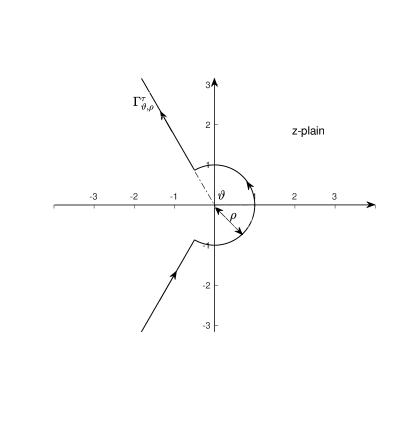
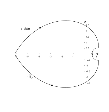
Figure 1: Contour $\Gamma_{\vartheta,\rho}^{\tau}$ in $z$-plain and $\mathcal{C}_{\vartheta,\rho}^{\tau}$ in $\zeta$-plain under the transformation $\zeta=e^{-z\tau}$.

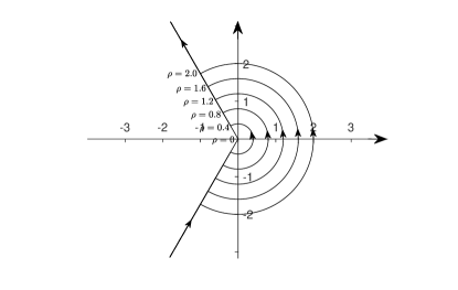
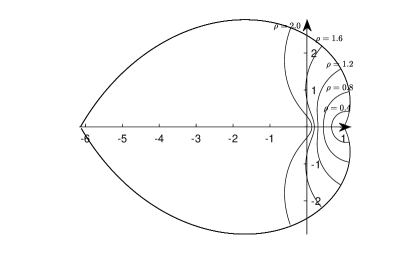
Figure 2: Contour $\Gamma_{\vartheta,\rho}^{\tau}$ in $z$-plain and $\mathcal{C}_{\vartheta,\rho}^{\tau}$ in $\zeta$-plain under the transformation $\zeta=e^{-z\tau}$ for different $\rho=0,0.4,0.8,1.2,1.6,2.0$, indicating $\mathbb{U}_{\vartheta,\rho_{1}}^{\tau}\subset\mathbb{U}_{\vartheta,\rho_{2}}^{\tau}$ provided $\rho_{1}\geq\rho_{2}$.

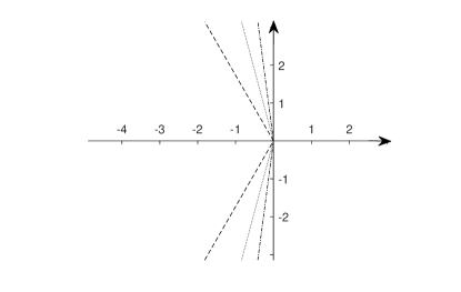
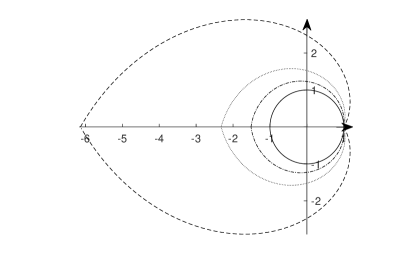
Figure 3: Contour $\Gamma_{\vartheta,0}^{\tau}$ in $z$-plain and $\mathcal{C}_{\vartheta,0}^{\tau}$ in $\zeta$-plain under the transformation $\zeta=e^{-z\tau}$ for different $\vartheta\in(\pi/2,\pi)$, indicating $\mathbb{U}_{\vartheta_{1}}\subset\mathbb{U}_{\vartheta_{2}}$ provided $\frac{\pi}{2}\leq\vartheta_{1}\leq\vartheta_{2}$.

2.4 Solution representation for $w_{h}(t)$

Let $\widehat{\phi}(z)$ be the Laplace transform of $\phi(t)$. Recalling that $\widehat{\partial_{t}^{\alpha}\phi}=z^{\alpha}\widehat{\phi}-z^{\alpha-1}\phi(0)$, we obtain $\widehat{D_{t}^{\alpha}w_{h}(t)}=\widehat{\partial_{t}^{\alpha}w_{h}(t)}=z^{\alpha}\widehat{w_{h}}$ thanks to $w_{h}(0)=0$. By taking the Laplace transform for (8), one gets

$$(z^{\alpha}-\Delta_{h})\widehat{w_{h}}=\widehat{g_{h}}+z^{-1}(\Delta_{h}v_{h}+f_{h}(0)).$$

Resorting to the inverse Laplace transform, we have

$$w_{h}(t)=\frac{1}{2\pi\mathrm{i}}\int_{\Gamma_{\vartheta,\rho}}e^{zt}\big{(}K(z)(\Delta_{h}v_{h}+f_{h}(0))+zK(z)\widehat{g_{h}}(z)\big{)}\mathrm{d}z,$$ (11)

where the function $K(z)$ stands for $K(z)=z^{-1}(z^{\alpha}-\Delta_{h})^{-1}$.

3 Nonstandard error estimates for ACN scheme

The standard analysis developed in jin2018analysis consists of solution representations of both the time continuous problem (8) and the discrete counterpart (10) where the latter requires the generating function $\omega(\zeta)$ be analytic and nonzero in the closed unit disc except for the point $\zeta=1$. Clearly, for the ACN scheme the function $\omega(\zeta)$ in (6) is zero at point $\zeta=-1$ and fails to meet this requirement. A key observation to surmount this problem is that $\widetilde{\omega}(\zeta)$ for the fractional BDF-2 or the generalized 2nd-order Newton–Gregory formula defined in (5) satisfies the requirement, and by using the residue theorem and the properties of $\mathbb{U}_{\vartheta}$ listed in Lemma 2, one can obtain the expression of the solution immediately.

Lemma 3

For $\widetilde{\omega}(\zeta)$ defined in (5), there exists some $\vartheta\in(\pi/2,\pi)$ such that

$$\begin{split}\big{\|}\big{(}\tau^{-\alpha}\widetilde{\omega}(\zeta)-\Delta_{h}\big{)}^{-1}\big{\|}\lesssim\tau^{\alpha}\big{|}\widetilde{\omega}(\zeta)\big{|}^{-1},\quad\forall\zeta\in\mathbb{U}_{\vartheta}.\end{split}$$

Proof

In accordance to (9), we only need to show that $\widetilde{\omega}(\zeta)$ belongs to $\Sigma_{\sigma}$ for some $\sigma\in(\pi/2,\pi)$. Indeed, the singular point of $\widetilde{\omega}(\zeta)$ for fractional BDF-2 (except for $\zeta=1$) is $\zeta=3$ and the zero for the generalized 2nd-order Newton–Gregory formula is $\zeta=1+\frac{2}{\alpha}$, both of which satisfy $|\zeta|>1$. By (iii) in Lemma 2, there exists some $\vartheta\in(\pi/2,\pi)$ such that $3\notin\mathbb{U}_{\vartheta}$ and $1+\frac{2}{\alpha}\notin\mathbb{U}_{\vartheta}$, meaning that $\widetilde{\omega}(\zeta)$ is analytic and nonzero in $\mathbb{U}_{\vartheta}$. Since it is well known that both methods are A$(\frac{\pi}{2})$-stable, i.e., $\widetilde{\omega}(\zeta)\in\Sigma_{\frac{\pi}{2}}$ for any $\zeta\in\mathbb{U}_{\frac{\pi}{2}}=\{z:|z|<1\}$ (see (ii) in Lemma 2), then by analyticity of $\widetilde{\omega}(\zeta)$ one gets $\widetilde{\omega}(\zeta)\in\Sigma_{\sigma}$ for some $\sigma\in(\pi/2,\pi)$ so long as $\vartheta$ is close to $\frac{\pi}{2}$ sufficiently.

Theorem 3.1

Given $\tau>0$ and $\alpha\in(0,1)$. There exist $\vartheta\in(\pi/2,\pi)$ and $\rho>0$ which are independent of $\tau$ such that the solution of the ACN scheme can be formulated by the following form

$$\begin{split}W_{h}^{n}&=\frac{1}{2\pi{\rm i}}\int_{\Gamma_{\vartheta,\rho}^{\tau}}e^{zt_{n}}\big{[}\tau\Phi_{i}(e^{-z\tau})(\Delta_{h}v_{h}+f_{h}(0))+\tau\Phi_{g}(e^{-z\tau})\widetilde{g}_{h}(e^{-z\tau})\big{]}\mathrm{d}z\\ &\quad-(-1)^{n}\big{(}\tau^{-\alpha}\widetilde{\omega}(-1)-\Delta_{h}\big{)}^{-1}\big{(}\Delta_{h}v_{h}+f_{h}(0)\big{)},\end{split}$$ (12)

where $\Phi_{i}(\zeta)$ and $\Phi_{g}(\zeta)$ are defined by

$$\begin{split}\Phi_{i}(\zeta)=\frac{2\zeta}{1-\zeta^{2}}\big{(}\tau^{-\alpha}\widetilde{\omega}(\zeta)-\Delta_{h}\big{)}^{-1},\quad\Phi_{g}(\zeta)=\big{(}\tau^{-\alpha}\widetilde{\omega}(\zeta)-\Delta_{h}\big{)}^{-1}.\end{split}$$ (13)

Proof

Multiplying both sides of (10) by $\zeta^{n}$ and summing the index $n$ from $1$ to $\infty$, one gets

$$\begin{split}\bigg{(}\tau^{-\alpha}\omega(\zeta)-\frac{1+\zeta}{2}\Delta_{h}\bigg{)}W_{h}(\zeta)=\frac{1+\zeta}{2}\widetilde{g}_{h}(\zeta)+\frac{\zeta}{1-\zeta}\big{(}f_{h}(0)+\Delta_{h}v_{h}\big{)},\end{split}$$ (14)

where we have used the following identity

$$\begin{split}\sum_{n=1}^{\infty}\zeta^{n}D_{\tau}^{\alpha}W_{h}^{n-\frac{1}{2}}=\tau^{-\alpha}\omega(\zeta)W_{h}(\zeta),\\ \frac{1}{2}\sum_{n=1}^{\infty}\zeta^{n}\big{(}\Delta_{h}W_{h}^{n}+\Delta_{h}W_{h}^{n-1}\big{)}=\frac{1+\zeta}{2}\Delta_{h}W_{h}(\zeta),\\ \frac{1}{2}\sum_{n=1}^{\infty}\zeta^{n}(g_{h}^{n}+g_{h}^{n-1})=\frac{1+\zeta}{2}\widetilde{g}_{h}(\zeta),\\ \sum_{n=1}^{\infty}\zeta^{n}\big{(}f_{h}(0)+\Delta_{h}v_{h}\big{)}=\frac{\zeta}{1-\zeta}\big{(}f_{h}(0)+\Delta_{h}v_{h}\big{)}.\end{split}$$

Clearly, (14) indicates that $\zeta\neq-1$. By multiplying both sides of (14) with $\frac{2}{1+\zeta}$, we have

$$\begin{split}\big{(}\tau^{-\alpha}\widetilde{\omega}(\zeta)-\Delta_{h}\big{)}W_{h}(\zeta)=\widetilde{g}_{h}(\zeta)+\frac{2\zeta}{1-\zeta^{2}}\big{(}f_{h}(0)+\Delta_{h}v_{h}\big{)},\end{split}$$

where the operator $\tau^{-\alpha}\widetilde{\omega}(\zeta)-\Delta_{h}$ is invertible for $\zeta\in\mathbb{U}_{\vartheta}$ for some $\vartheta\in(\pi/2,\pi)$, due to Lemma 3. We therefore obtained the following relation, with $\Phi_{i}(\zeta)$ and $\Phi_{g}(\zeta)$ defined in (13), that

$$\begin{split}W_{h}(\zeta)=\Phi_{i}(\zeta)\big{(}\Delta_{h}v_{h}+f_{h}(0)\big{)}+\Phi_{g}(\zeta)\widetilde{g}_{h}(\zeta),\quad\forall\zeta\in\mathbb{U}_{\vartheta}\setminus\{-1\}.\end{split}$$ (15)

For an appropriately chosen $\rho>0$, the result (ii) in Lemma 1 tells us $\mathbb{U}_{\vartheta,\rho}^{\tau}\subset\mathbb{U}_{\vartheta,0}^{\tau}=\mathbb{U}_{\vartheta}$, implying that $(\ref{bdf.2.2})$ also holds for $\zeta\in\mathbb{U}_{\vartheta,\rho}^{\tau}\setminus\{-1\}$. Using the residue theorem, one gets immediately that

$$\begin{split}-\frac{1}{2\pi{\rm i}}\int_{\mathcal{C}_{\vartheta,\rho}^{\tau}}\frac{W_{h}(\zeta)}{\zeta^{n+1}}\mathrm{d}\zeta={\rm Res}\bigg{(}\frac{W_{h}(\zeta)}{\zeta^{n+1}},0\bigg{)}+{\rm Res}\bigg{(}\frac{W_{h}(\zeta)}{\zeta^{n+1}},-1\bigg{)},\end{split}$$ (16)

where the first term of the right side of the equation is exactly $W_{h}^{n}$, and the second term can further be formulated as

$$\begin{split}{\rm Res}\bigg{(}\frac{W_{h}(\zeta)}{\zeta^{n+1}},-1\bigg{)}&=(-1)^{n-1}{\rm Res}\big{(}\Phi_{i}(\zeta),-1\big{)}(\Delta_{h}v_{h}+f_{h}(0))\\ &=(-1)^{n}\big{(}\tau^{-\alpha}\widetilde{\omega}(-1)-\Delta_{h}\big{)}^{-1}\big{(}\Delta_{h}v_{h}+f_{h}(0)\big{)}.\end{split}$$ (17)

By setting $\zeta=e^{-z\tau}$, the term of the left side of (16) reads that

$$\begin{split}-\frac{1}{2\pi{\rm i}}\int_{\mathcal{C}_{\vartheta,\rho}^{\tau}}\frac{W_{h}(\zeta)}{\zeta^{n+1}}\mathrm{d}\zeta=\frac{1}{2\pi{\rm i}}\int_{\Gamma_{\vartheta,\rho}^{\tau}}e^{zt_{n}}\big{[}\tau\Phi_{i}(e^{-z\tau})(\Delta_{h}v_{h}+f_{h}(0))+\tau\Phi_{g}(e^{-z\tau})\widetilde{g}_{h}(e^{-z\tau})\big{]}\mathrm{d}z,\end{split}$$

which, combined with (17), completes the proof of the theorem.

The next lemma is from Lemma B.1 in jin2017correction and Lemma 2 in wang2020higher (Actually, Lemma 2 in jin2017correction indicates that (18) holds for any $z\in\Gamma_{\vartheta,0}^{\tau}$. By introducing a positive $\rho$, one can check readily (18) still holds and the proof is omitted here).

Lemma 4

Given $\tau>0$. For $\widetilde{\omega}(\zeta)$ defined in (5), there exist some $\vartheta^{\prime}\in(\pi/2,\pi)$ and $\rho>0$ which are independent of $\tau$, such that

$$\tau^{\alpha}|z|^{\alpha}\lesssim|\widetilde{\omega}(e^{-z\tau})|\lesssim\tau^{\alpha}|z|^{\alpha},\quad\forall\vartheta\in(\pi/2,\vartheta^{\prime}),\quad\forall z\in\Gamma_{\vartheta,\rho}^{\tau}.$$ (18)

In combination with Lemma 3 and Lemma 4, we obtain

$$\big{\|}\big{(}\tau^{-\alpha}\widetilde{\omega}(e^{-z\tau})-\Delta_{h}\big{)}^{-1}\big{\|}\lesssim|z|^{-\alpha},\quad\forall z\in\Gamma_{\vartheta,\rho}^{\tau},$$ (19)

where $\vartheta\in(\pi/2,\pi)$ and $\rho>0$ are some constants free of $\tau$.

Lemma 5

Given $\tau>0$. Let $\widetilde{\omega}(\zeta)$ be defined in (5). There exist some $\vartheta^{\prime}\in(\pi/2,\pi)$ and $\rho>0$ which are independent of $\tau$, such that

$$|z^{\alpha}-\tau^{-\alpha}\widetilde{\omega}(e^{-z\tau})|\lesssim\tau^{2}|z|^{2+\alpha},\quad\forall\vartheta\in(\pi/2,\vartheta^{\prime}),\quad\forall z\in\Gamma_{\vartheta,\rho}^{\tau}.$$ (20)

Proof

For the fractional BDF-2, Lemma B.1 in jin2017correction has shown (20) holds. The technique can also be applied to the GNG-2 similarly and the details are omitted here.

Lemma 6

Given $\tau>0$, there exist some $\vartheta\in(\pi/2,\pi)$ and $\rho>0$ which are independent of $\tau$ such that

• $\displaystyle\bigg{|}\frac{2e^{-z\tau}}{1-e^{-2z\tau}}-z^{-1}\tau^{-1}\bigg{|}\lesssim\tau|z|,\quad\bigg{|}\frac{e^{-z\tau}}{(1-e^{-z\tau})^{2}}-z^{-2}\tau^{-2}\bigg{|}\lesssim 1,\quad\forall z\in\Gamma_{\vartheta,\rho}^{\tau}$.

• $\|\tau\Phi_{i}(e^{-z\tau})-K(z)\|\lesssim\tau^{2}|z|^{1-\alpha},\quad\forall z\in\Gamma_{\vartheta,\rho}^{\tau}$.

• $\displaystyle\bigg{\|}\frac{\tau^{2}e^{-z\tau}}{(1-e^{-z\tau})^{2}}\Phi_{g}(e^{-z\tau})-z^{-1}K(z)\bigg{\|}\lesssim\tau^{2}|z|^{-\alpha},\quad\forall z\in\Gamma_{\vartheta,\rho}^{\tau},$

where $K(z)=z^{-1}(z^{\alpha}-\Delta_{h})^{-1}$ and $\Phi_{i}(\zeta)$ and $\Phi_{g}(\zeta)$ are defined in (13).

Proof

For (i), if $|z|\tau<\epsilon$ where $\epsilon>0$ is given small enough, by using the Taylor expansion of $e^{-z\tau}$, one can check (i) holds readily. To be specific, denote by $Q_{n}(z)$ some function which may not be the same at different occurrence, fulfilling $|Q_{n}(z)|\lesssim|z|^{n}$ for sufficiently small $|z|$. There holds

$$\begin{split}\frac{2z\tau e^{-z\tau}}{1-e^{-2z\tau}}&=\frac{2z\tau\big{(}1-z\tau+z^{2}\tau^{2}/2+Q_{3}(z\tau)\big{)}}{1-\big{(}1-2z\tau+2z^{2}\tau^{2}+Q_{3}(z\tau)\big{)}}=\frac{1-z\tau+z^{2}\tau^{2}/2+Q_{3}(z\tau)}{1-z\tau-Q_{2}(z\tau)}\\ &=1+\frac{z^{2}\tau^{2}/2+Q_{3}(z\tau)+Q_{2}(z\tau)}{1-z\tau-Q_{2}(z\tau)}=1+Q_{2}(z\tau),\end{split}$$

which leads to

$$\bigg{|}\frac{2e^{-z\tau}}{1-e^{-2z\tau}}-z^{-1}\tau^{-1}\bigg{|}=|z|^{-1}\tau^{-1}\bigg{|}\frac{2z\tau e^{-z\tau}}{1-e^{-2z\tau}}-1\bigg{|}=|z|^{-1}\tau^{-1}Q_{2}(z\tau)\lesssim\tau|z|.$$

To prove the second inequality of (i), we note that

$$\begin{split}\frac{z^{2}\tau^{2}e^{-z\tau}}{(1-e^{-z\tau})^{2}}&=\frac{1-z\tau+z^{2}\tau^{2}/2+Q_{3}(z\tau)}{(1-z\tau/2-Q_{2}(z\tau))^{2}}=\frac{1-z\tau+z^{2}\tau^{2}/2+Q_{3}(z\tau)}{1-z\tau+Q_{2}(z\tau)}\\ &=1+\frac{Q_{2}(z\tau)}{1-z\tau+Q_{2}(z\tau)},\end{split}$$

yielding

$$\bigg{|}\frac{e^{-z\tau}}{(1-e^{-z\tau})^{2}}-z^{-2}\tau^{-2}\bigg{|}=|z|^{-2}\tau^{-2}\bigg{|}\frac{z^{2}\tau^{2}e^{-z\tau}}{(1-e^{-z\tau})^{2}}-1\bigg{|}\lesssim 1.$$

If $|z|\tau\geq\epsilon$, let $z=re^{\pm{\rm i}\vartheta}$ with $r\in[\frac{\epsilon}{\tau},\frac{\pi}{\tau\sin\vartheta}]$ for some $\vartheta\in(\pi/2,\pi)$ to be determined next. We only need to prove that the left terms of the inequalities in (i) can be bounded by some positive constants (independent of $\tau$), since any positive constant satisfies $c\leq\frac{c}{\epsilon}\epsilon\leq\frac{c}{\epsilon}|z|\tau$ by the assumption.

Let $\vartheta^{\prime},\vartheta^{\prime\prime}\in(\pi/2,\pi)$ be given and sufficiently close to $\pi/2$ with $\vartheta^{\prime}<\vartheta^{\prime\prime}$. For any $\vartheta\in(\vartheta^{\prime},\vartheta^{\prime\prime})$, using the following estimates,

$$\begin{split}|e^{-z\tau}|&\leq e^{|z|\tau}\leq e^{\frac{\pi}{\sin\vartheta}}\leq e^{\frac{\pi}{\sin\vartheta^{\prime\prime}}},\quad|z^{-1}\tau^{-1}|\leq\frac{1}{\epsilon},\\ \big{|}1-e^{-z\tau}\big{|}^{2}&=(1-e^{-\tau r\cos\vartheta})^{2}+2e^{-\tau r\cos 2\vartheta}[1-\cos(\tau r\sin\vartheta)]\\ &\geq(e^{\tau r\sin(\vartheta-\pi/2)}-1)^{2}\geq\tau^{2}r^{2}\sin^{2}(\vartheta-\pi/2)\\ &\geq\epsilon^{2}\sin^{2}(\vartheta^{\prime}-\pi/2),\\ \big{|}1-e^{-2z\tau}\big{|}^{2}&\geq 4\tau^{2}r^{2}\sin^{2}(\vartheta-\pi/2)\geq 4\epsilon^{2}\sin^{2}(\vartheta^{\prime}-\pi/2),\end{split}$$

one can get

$$\bigg{|}\frac{2e^{-z\tau}}{1-e^{-2z\tau}}-z^{-1}\tau^{-1}\bigg{|}\lesssim\frac{|e^{-z\tau}|}{|1-e^{-2z\tau}|}+\frac{1}{|z\tau|}\lesssim\frac{e^{\frac{\pi}{\sin\vartheta^{\prime\prime}}}}{2\epsilon\sin(\vartheta^{\prime}-\pi/2)}+\frac{1}{\epsilon},$$

and

$$\bigg{|}\frac{e^{-z\tau}}{(1-e^{-z\tau})^{2}}-z^{-2}\tau^{-2}\bigg{|}\lesssim\frac{|e^{-z\tau}|}{|1-e^{-z\tau}|^{2}}+\frac{1}{|z\tau|^{2}}\lesssim\frac{e^{\frac{\pi}{\sin\vartheta^{\prime\prime}}}}{\epsilon^{2}\sin^{2}(\vartheta^{\prime}-\pi/2)}+\frac{1}{\epsilon^{2}}.$$

For (ii), we have, by the definition of $\Phi_{i}$ and $K(z)$ that

$$\begin{split}\tau\Phi_{i}(e^{-z\tau})-K(z)&=\tau\bigg{(}\frac{2e^{-z\tau}}{1-e^{-2z\tau}}-z^{-1}\tau^{-1}\bigg{)}\big{(}\tau^{-\alpha}\widetilde{\omega}(e^{-z\tau})-\Delta_{h}\big{)}^{-1}\\ &\quad+z^{-1}\big{[}\big{(}\tau^{-\alpha}\widetilde{\omega}(e^{-z\tau})-\Delta_{h}\big{)}^{-1}-(z^{\alpha}-\Delta_{h})^{-1}\big{]}.\end{split}$$ (21)

In accordance to the following identity

$$\begin{split}&\quad\big{(}\tau^{-\alpha}\widetilde{\omega}(e^{-z\tau})-\Delta_{h}\big{)}^{-1}-(z^{\alpha}-\Delta_{h})^{-1}\\ &=\big{(}\tau^{-\alpha}\widetilde{\omega}(e^{-z\tau})-\Delta_{h}\big{)}^{-1}\big{(}z^{\alpha}-\tau^{-\alpha}\widetilde{\omega}(e^{-z\tau})\big{)}(z^{\alpha}-\Delta_{h})^{-1},\end{split}$$ (22)

and the estimates in (i), (19), (20) and (9), by (21) one immediately gets

$$\|\tau\Phi_{i}(e^{-z\tau})-K(z)\|\lesssim\tau^{2}|z|^{1-\alpha}.$$

For (iii), with $\Phi_{g}$ defined in (13), we have

$$\begin{split}\frac{\tau^{2}e^{-z\tau}}{(1-e^{-z\tau})^{2}}\Phi_{g}(e^{-z\tau})-z^{-1}K(z)&=\tau^{2}\bigg{[}\frac{e^{-z\tau}}{(1-e^{-z\tau})^{2}}-z^{-2}\tau^{-2}\bigg{]}\big{(}\tau^{-\alpha}\widetilde{\omega}(e^{-z\tau})-\Delta_{h}\big{)}^{-1}\\ &\quad+z^{-2}\big{[}\big{(}\tau^{-\alpha}\widetilde{\omega}(e^{-z\tau})-\Delta_{h}\big{)}^{-1}-(z^{\alpha}-\Delta_{h})^{-1}\big{]},\end{split}$$

which, in combination with the identity (LABEL:bdf.4.2.3) and (i), (19), (20) and (9), yields

$$\bigg{\|}\frac{\tau^{2}e^{-z\tau}}{(1-e^{-z\tau})^{2}}\Phi_{g}(e^{-z\tau})-z^{-1}K(z)\bigg{\|}\lesssim\tau^{2}|z|^{-\alpha}.$$

Since the source term $f(x,t)$ can be expanded as $f(x,t)=q_{0}(x)+tq_{1}(x)+t*q(x,t)$, the sharp error analysis for the ACN scheme consists of the following several theorems.

Theorem 3.2

Assume $f(x,t)\equiv 0$. Let $W_{h}^{n}$ be the solution of (10) and $U_{h}^{n}:=W_{h}^{n}+u_{h}(0)$ be the approximation to $u_{h}(t_{n})$ for $n\geq 1$. For sufficiently small $\tau>0$, there holds

$$\|u_{h}(t_{n})-U_{h}^{n}\|_{L^{2}(\Omega)}\lesssim(t_{n}^{\alpha-2}\tau^{2}+\tau^{\alpha})\|\Delta u_{0}\|_{L^{2}(\Omega)}.$$

Proof

By definition we have $u_{h}(t_{n})-U_{h}^{n}=w_{h}(t_{n})-W_{h}^{n}$. Using the solution representations (11) and (12), there holds

$$\begin{split}w_{h}(t_{n})-W_{h}^{n}=I_{1}^{n}+I_{2}^{n}+I_{3}^{n},\end{split}$$

where $I_{i}^{n}(i=1,2,3)$ stand for

$$\begin{split}I_{1}^{n}&=\frac{1}{2\pi{\rm i}}\int_{\Gamma_{\vartheta,\rho}^{\tau}}e^{zt_{n}}\big{[}K(z)-\tau\Phi_{i}(e^{-z\tau})\big{]}\Delta_{h}v_{h}\mathrm{d}z,\\ I_{2}^{n}&=\frac{1}{2\pi{\rm i}}\int_{\Gamma_{\vartheta,\rho}\setminus\Gamma_{\vartheta,\rho}^{\tau}}e^{zt_{n}}K(z)\Delta_{h}v_{h}\mathrm{d}z,\\ I_{3}^{n}&=(-1)^{n}\big{(}\tau^{-\alpha}\widetilde{\omega}(-1)-\Delta_{h}\big{)}^{-1}\Delta_{h}v_{h}.\end{split}$$

For the term $I_{1}^{n}$, by appealing to the estimate (ii) in Lemma 6 and the symmetry of contour $\Gamma_{\vartheta,\rho}^{\tau}$, we have

$$\begin{split}\|I_{1}^{n}\|_{L^{2}(\Omega)}&\lesssim\tau^{2}\|\Delta_{h}v_{h}\|_{L^{2}(\Omega)}\int_{\Gamma_{\vartheta,\rho}^{\tau}}|e^{zt_{n}}||z|^{1-\alpha}|\mathrm{d}z|\\ &\lesssim\tau^{2}\|\Delta_{h}v_{h}\|_{L^{2}(\Omega)}\bigg{(}\int_{\rho}^{\frac{\pi}{\tau\sin\vartheta}}e^{rt_{n}\cos\vartheta}r^{1-\alpha}\mathrm{d}r+\rho^{2-\alpha}\int_{0}^{\vartheta}e^{\rho t_{n}\cos\theta}\mathrm{d}\theta\bigg{)}.\end{split}$$ (23)

Taking $s=rt_{n}$, the first integration in (23) reads that

$$\int_{\rho}^{\frac{\pi}{\tau\sin\vartheta}}e^{rt_{n}\cos\vartheta}r^{1-\alpha}\mathrm{d}r\leq t_{n}^{\alpha-2}\int_{0}^{+\infty}e^{s\cos\vartheta}s^{1-\alpha}\mathrm{d}s\lesssim t_{n}^{\alpha-2},$$ (24)

where the last inequality holds for that $\vartheta\in(\pi/2,\pi)$ and $e^{s\cos\vartheta}$ decays faster than $s^{1-\alpha}$ at infinity. By choosing $\rho$ such that $\rho t_{n}\leq 1$, the second integration in (23) can further be formulated as

$$\rho^{2-\alpha}\int_{0}^{\vartheta}e^{\rho t_{n}\cos\theta}\mathrm{d}\theta\leq t_{n}^{\alpha-2}\int_{0}^{\vartheta}e\mathrm{d}\theta\lesssim t_{n}^{\alpha-2},$$

which, in combination with (24) and (23), leads to

$$\|I_{1}^{n}\|_{L^{2}(\Omega)}\lesssim t_{n}^{\alpha-2}\tau^{2}\|\Delta_{h}v_{h}\|_{L^{2}(\Omega)}.$$

For the term $I_{2}^{n}$, since $\|K(z)\|=\|z^{-1}(z^{\alpha}-\Delta_{h})^{-1}\|\lesssim|z|^{-1-\alpha}$, we obtain

$$\begin{split}\|I_{2}^{n}\|_{L^{2}(\Omega)}&\lesssim\|\Delta_{h}v_{h}\|_{L^{2}(\Omega)}\int_{\frac{\pi}{\tau\sin\vartheta}}^{+\infty}e^{rt_{n}\cos\vartheta}r^{-1-\alpha}\mathrm{d}r\lesssim\tau^{2}\|\Delta_{h}v_{h}\|_{L^{2}(\Omega)}\int_{\frac{\pi}{\tau\sin\vartheta}}^{+\infty}e^{rt_{n}\cos\vartheta}r^{1-\alpha}\mathrm{d}r\\ &\lesssim t_{n}^{\alpha-2}\tau^{2}\|\Delta_{h}v_{h}\|_{L^{2}(\Omega)},\end{split}$$ (25)

where the last inequality is worked out by setting $s=rt_{n}$ and the fast decay of $e^{s\cos\vartheta}$ as $s$ tends to infinity.
For the term $I_{3}^{n}$, direct estimate shows that

$$\|I_{3}^{n}\|_{L^{2}(\Omega)}\lesssim\tau^{\alpha}\|\Delta_{h}v_{h}\|_{L^{2}(\Omega)}.$$ (26)

Combining (23), (25) with (26) and using the identity $\Delta_{h}R_{h}=P_{h}\Delta$, we complete the proof of the theorem.

Theorem 3.3

Assume $u_{0}(x)\equiv 0$ and $f(x,t)=q_{0}(x)+tq_{1}(x)$ with $q_{0},q_{1}\in L^{2}(\Omega)$. Let $W_{h}^{n}$ be the solution of (10) and $U_{h}^{n}:=W_{h}^{n}+u_{h}(0)$ be the approximation to $u_{h}(t_{n})$ for $n\geq 1$. For sufficiently small $\tau>0$, there holds

$$\|u_{h}(t_{n})-U_{h}^{n}\|_{L^{2}(\Omega)}\lesssim\tau^{2}\big{(}t_{n}^{\alpha-2}\|q_{0}(x)\|_{L^{2}(\Omega)}+t_{n}^{\alpha-1}\|q_{1}(x)\|_{L^{2}(\Omega)}\big{)}+\tau^{\alpha}\|q_{0}(x)\|_{L^{2}(\Omega)}.$$

Proof

For $f(x,t)=q_{0}(x)+tq_{1}(x)$, we have $f_{h}(0)=q_{0h}(x):=P_{h}q_{0}(x)$, $g_{h}(x,t)=tq_{1h}(x):=tP_{h}q_{1}(x)$ and

$$\widetilde{g}_{h}(\zeta)=q_{1h}(x)\sum_{i=0}^{\infty}t_{i}\zeta^{i}=\frac{\tau\zeta}{(1-\zeta)^{2}}q_{1h}(x),\quad\widehat{g_{h}}(z)=z^{-2}q_{1h}(x).$$

It is notable that if $q_{1}(x)\equiv 0$, by almost the same estimate as Theorem 3.2, one can obtain

$$\|u_{h}(t_{n})-U_{h}^{n}\|_{L^{2}(\Omega)}\lesssim(t_{n}^{\alpha-2}\tau^{2}+\tau^{\alpha})\|q_{0}(x)\|_{L^{2}(\Omega)}.$$

We therefore in the next analysis mainly focus on $q_{0}(x)\equiv 0$. By solution representations (11) and (12), we have

$$\begin{split}w_{h}(t_{n})-W_{h}^{n}=J_{1}^{n}+J_{2}^{n},\end{split}$$ (27)

where $J_{i}^{n}(i=1,2)$ stand for

$$\begin{split}J_{1}^{n}&=\frac{1}{2\pi{\rm i}}\int_{\Gamma_{\vartheta,\rho}^{\tau}}e^{zt_{n}}\big{(}zK(z)\widehat{g_{h}}(z)-\tau\Phi_{g}(e^{-z\tau})\widetilde{g}_{h}(e^{-z\tau})\big{)}\mathrm{d}z,\\ J_{2}^{n}&=\frac{1}{2\pi{\rm i}}\int_{\Gamma_{\vartheta,\rho}\setminus\Gamma_{\vartheta,\rho}^{\tau}}e^{zt_{n}}zK(z)\widehat{g_{h}}(z)\mathrm{d}z.\end{split}$$

For the term $J_{1}^{n}$, by resorting to the estimate (iii) in Lemma 6 and the symmetry of contour $\Gamma_{\vartheta,\rho}^{\tau}$, we have

$$\begin{split}\|J_{1}^{n}\|_{L^{2}(\Omega)}&\lesssim\tau^{2}\|q_{1h}(x)\|_{L^{2}(\Omega)}\bigg{(}\int_{\rho}^{\frac{\pi}{\tau\sin\vartheta}}e^{rt_{n}\cos\vartheta}r^{-\alpha}\mathrm{d}r+\rho^{1-\alpha}\int_{0}^{\vartheta}e^{\rho t_{n}\cos\theta}\mathrm{d}\theta\bigg{)}\\ &\lesssim t_{n}^{\alpha-1}\tau^{2}\|q_{1h}(x)\|_{L^{2}(\Omega)},\end{split}$$ (28)

where the replacement $s=rt_{n}$ and assumption $\rho t_{n}\leq 1$ are adopt in deriving the last inequality.
For the term $J_{2}^{n}$, since $\|zK(z)\widehat{g_{h}}(z)\|_{L^{2}(\Omega)}=\|z^{-1}K(z)q_{1h}(x)\|_{L^{2}(\Omega)}\lesssim|z|^{-2-\alpha}\|q_{1h}(x)\|_{L^{2}(\Omega)}$, one gets

$$\begin{split}\|J_{2}^{n}\|_{L^{2}(\Omega)}&\lesssim\|q_{1h}(x)\|_{L^{2}(\Omega)}\int_{\frac{\pi}{\tau\sin\vartheta}}^{+\infty}e^{rt_{n}\cos\vartheta}r^{-2-\alpha}\mathrm{d}r\lesssim\tau^{2}\|\Delta_{h}v_{h}\|_{L^{2}(\Omega)}\int_{\frac{\pi}{\tau\sin\vartheta}}^{+\infty}e^{rt_{n}\cos\vartheta}r^{-\alpha}\mathrm{d}r\\ &\lesssim t_{n}^{\alpha-1}\tau^{2}\|q_{1h}(x)\|_{L^{2}(\Omega)}.\end{split}$$ (29)

Combining (27), (28) with (29) and using the fact that $\|q_{1h}(x)\|_{L^{2}(\Omega)}\leq\|q_{1}(x)\|_{L^{2}(\Omega)}$, we get

$$\|w_{h}(t_{n})-W_{h}^{n}\|_{L^{2}(\Omega)}\lesssim t_{n}^{\alpha-1}\tau^{2}\|q_{1h}(x)\|_{L^{2}(\Omega)}.$$

The proof of the theorem is completed.

Remark 2

Theorem 3.3 indicates that if the source term $f(x,t)$ is smooth and is zero at time $t=0$, such as $f=tq_{1}(x)$, then the error at $t_{n}$ is of $O(\tau^{2})$. See Example 2 in Section 5 for verification.

Theorem 3.4

Assume $u_{0}(x)\equiv 0$ and $f(x,t)=t*q(x,t)$. Let $W_{h}^{n}$ be the solution of (10) and $U_{h}^{n}:=W_{h}^{n}+u_{h}(0)$ be the approximation to $u_{h}(t_{n})$ for $n\geq 1$. For sufficiently small $\tau>0$, there holds

$$\|u_{h}(t_{n})-U_{h}^{n}\|_{L^{2}(\Omega)}\lesssim\tau^{2}\int_{0}^{t_{n}}(t_{n}-s)^{\alpha-1}\|q(s)\|_{L^{2}(\Omega)}\mathrm{d}s.$$ (30)

Proof

In this case, the discrete solution representation in (12) consists only the integral part. The estimate (30) can be carried out using the same analysis as Lemma 3.12 in jin2018analysis which is omitted here.

Remark 3

Combining Theorem 3.2-Theorem 3.4, we actually have shown the following result that, by assuming $u_{0}(x)\in D(\Delta)$, $f(x,t)\in W^{1,\infty}(0,T;L^{2}(\Omega))$, $\int_{0}^{t}(t-s)^{\alpha-1}\|f^{\prime\prime}(s)\|_{L^{2}(\Omega)}\mathrm{d}s<\infty$, and letting $W_{h}^{n}$ be the solution of (10) and $U_{h}^{n}:=W_{h}^{n}+u_{h}(0)$ be the approximation to $u_{h}(t_{n})$ for $n\geq 1$, then for sufficiently small $\tau>0$, there holds

$$\begin{split}\|u_{h}(t_{n})-U_{h}^{n}\|_{L^{2}(\Omega)}&\lesssim\tau^{2}\bigg{(}t_{n}^{\alpha-2}(\|f(0)\|_{L^{2}(\Omega)}+\|\Delta u_{0}\|_{L^{2}(\Omega)})+t_{n}^{\alpha-1}\|f^{\prime}(0)\|_{L^{2}(\Omega)}\\ &\quad+\int_{0}^{t_{n}}(t_{n}-s)^{\alpha-1}\|f^{\prime\prime}(s)\|_{L^{2}(\Omega)}\mathrm{d}s\bigg{)}+\tau^{\alpha}(\|\Delta u_{0}\|_{L^{2}(\Omega)}+\|f(0)\|_{L^{2}(\Omega)}).\end{split}$$

4 Correction method for ACN scheme

In this section we derive the modified averaging Crank-Nicolson (MACN) scheme by adding corrections to obtain the optimal accuracy. In general, at least two time steps should be modified (in which case at least two parameters are involved) since the singularity of $\Phi_{i}(\zeta)$ at $\zeta=-1$ must be removed and some estimate, such as (35) in the following analysis, should be satisfied. Define $a^{(1)}$ and $a^{(2)}$ as the correction parameters, with which the modified ACN scheme can be formulated as

$$\begin{split}D_{\tau}^{\alpha}W_{h}^{\frac{1}{2}}-\frac{1}{2}\Delta_{h}W_{h}^{1}=\frac{1}{2}\big{(}f_{h}^{1}+f_{h}(0)\big{)}+\Delta_{h}v_{h}+a^{(1)}(f_{h}(0)+\Delta_{h}v_{h}),\quad&n=1,\\ D_{\tau}^{\alpha}W_{h}^{\frac{3}{2}}-\frac{1}{2}\big{(}\Delta_{h}W_{h}^{2}+\Delta_{h}W_{h}^{1}\big{)}=\frac{1}{2}\big{(}f_{h}^{2}+f_{h}^{1}\big{)}+\Delta_{h}v_{h}+a^{(2)}(f_{h}(0)+\Delta_{h}v_{h}),\quad&n=2,\\ D_{\tau}^{\alpha}W_{h}^{n-\frac{1}{2}}-\frac{1}{2}\big{(}\Delta_{h}W_{h}^{n}+\Delta_{h}W_{h}^{n-1}\big{)}=\frac{1}{2}\big{(}f_{h}^{n}+f_{h}^{n-1}\big{)}+\Delta_{h}v_{h},\quad&n\geq 3.\end{split}$$ (31)

Theorem 4.1

Given $\tau>0$ and $\alpha\in(0,1)$. There exist $\vartheta\in(\pi/2,\pi)$ and $\rho>0$ which are independent of $\tau$, such that the solution of the modified ACN scheme (for some carefully chosen $a^{(1)}$ and $a^{(2)}$) takes the form

$$\begin{split}W_{h}^{n}&=\frac{1}{2\pi{\rm i}}\int_{\Gamma_{\vartheta,\rho}^{\tau}}e^{zt_{n}}\big{[}\tau\Phi_{mi}(e^{-z\tau})(\Delta_{h}v_{h}+f_{h}(0))+\tau\Phi_{g}(e^{-z\tau})\widetilde{g}_{h}(e^{-z\tau})\big{]}\mathrm{d}z\end{split}$$

where $\Phi_{g}(\zeta)$ is defined in (13) and $\Phi_{mi}(\zeta)$ is defined by

$$\begin{split}\Phi_{mi}(\zeta)=\frac{2\zeta}{1+\zeta}\bigg{(}\frac{1}{1-\zeta}+a^{(1)}+a^{(2)}\zeta\bigg{)}\big{(}\tau^{-\alpha}\widetilde{\omega}(\zeta)-\Delta_{h}\big{)}^{-1}.\end{split}$$

Proof

Multiplying both sides of (31) by $\zeta^{n}$ and summing the index $n$ from $1$ to $\infty$, one gets

$$\begin{split}\big{(}\tau^{-\alpha}\widetilde{\omega}(\zeta)-\Delta_{h}\big{)}W_{h}(\zeta)&=\widetilde{g}_{h}(\zeta)+\frac{2\zeta}{1+\zeta}\bigg{(}\frac{1}{1-\zeta}+a^{(1)}+a^{(2)}\zeta\bigg{)}\big{(}f_{h}(0)+\Delta_{h}v_{h}\big{)},\end{split}$$

which leads to

$$\begin{split}W_{h}(\zeta)&=\frac{2\zeta}{1+\zeta}\bigg{(}\frac{1}{1-\zeta}+a^{(1)}+a^{(2)}\zeta\bigg{)}\big{(}\tau^{-\alpha}\widetilde{\omega}(\zeta)-\Delta_{h}\big{)}^{-1}\big{(}f_{h}(0)+\Delta_{h}v_{h}\big{)}\\ &\quad+\big{(}\tau^{-\alpha}\widetilde{\omega}(\zeta)-\Delta_{h}\big{)}^{-1}\widetilde{g}_{h}(\zeta)\\ &=\Phi_{mi}(\zeta)\big{(}f_{h}(0)+\Delta_{h}v_{h}\big{)}+\Phi_{g}(\zeta)\widetilde{g}_{h}(\zeta).\end{split}$$ (32)

For carefully chosen $a^{(1)}$ and $a^{(2)}$ such that the term $\frac{2\zeta}{1+\zeta}\big{(}\frac{1}{1-\zeta}+a^{(1)}+a^{(2)}\zeta\big{)}$ is analytic at $\zeta=-1$, i.e., by requiring that

$$\begin{split}\frac{1}{2}+a^{(1)}-a^{(2)}=0,\end{split}$$ (33)

we conclude (32) holds for any $\zeta\in\mathbb{U}^{\tau}_{\vartheta,\rho}$ for some $\vartheta\in(\pi/2,\pi)$ and $\rho>0$. Using the residue theorem, we obtain that

$$\begin{split}-\frac{1}{2\pi{\rm i}}\int_{\mathcal{C}_{\vartheta,\rho}^{\tau}}\frac{W_{h}(\zeta)}{\zeta^{n+1}}\mathrm{d}\zeta={\rm Res}\bigg{(}\frac{W_{h}(\zeta)}{\zeta^{n+1}},0\bigg{)}=W_{h}^{n}.\end{split}$$ (34)

Then, by setting $\zeta=e^{-z\tau}$ in (34) we completes the proof of the theorem.

Considering (33), $\Phi_{mi}$ can be reformulated as

$$\begin{split}\Phi_{mi}(\zeta)=\frac{2\zeta}{1-\zeta}\bigg{[}1+a^{(1)}-\bigg{(}a^{(1)}+\frac{1}{2}\bigg{)}\zeta\bigg{]}\big{(}\tau^{-\alpha}\widetilde{\omega}(\zeta)-\Delta_{h}\big{)}^{-1}.\end{split}$$

To determine $a^{(1)}$, one needs to justify the estimate (counterpart of (ii) in Lemma 6)

$$\begin{split}\big{\|}\tau\Phi_{mi}(e^{-z\tau})-z^{-1}(z^{\alpha}-\Delta_{h})^{-1}\big{\|}\lesssim\tau^{2}|z|^{1-\alpha},\quad\forall z\in\Gamma_{\vartheta,\rho}^{\tau},\end{split}$$ (35)

for some $\vartheta\in(\pi/2,\pi)$ and $\rho>0$, which leads to the following lemma.

Lemma 7

The estimate (35) holds if and only if $a^{(1)}=-\frac{1}{4}$.

Proof

For sufficiently small $\tau$, both of the fractional BDF-2 and GNG-2 satisfy (4) with $p=2$, indicating that for $|z|\tau<\epsilon$ where $\epsilon$ is chosen sufficiently small, there holds

$$\begin{split}\big{|}z^{\alpha}-\tau^{-\alpha}\widetilde{\omega}(e^{-z\tau})\big{|}\lesssim\tau^{2}|z|^{2+\alpha}.\end{split}$$

Appealing to the fact

$$\begin{split}&\quad\tau\Phi_{mi}(e^{-z\tau})-z^{-1}(z^{\alpha}-\Delta_{h})^{-1}\\ &=\bigg{\{}\frac{2\tau e^{-z\tau}}{1-e^{-z\tau}}\bigg{[}1+a^{(1)}-\bigg{(}a^{(1)}+\frac{1}{2}\bigg{)}e^{-z\tau}\bigg{]}-z^{-1}\bigg{\}}\big{(}\tau^{-\alpha}\widetilde{\omega}(e^{-z\tau})-\Delta_{h}\big{)}^{-1}\\ &\quad+z^{-1}\bigg{[}\big{(}\tau^{-\alpha}\widetilde{\omega}(e^{-z\tau})-\Delta_{h}\big{)}^{-1}-(z^{\alpha}-\Delta_{h})^{-1}\bigg{]},\end{split}$$

and using the identity (LABEL:bdf.4.2.3), one immediately gets

$$\begin{split}\big{|}\tau\Phi_{mi}(e^{-z\tau})-z^{-1}(z^{\alpha}-\Delta_{h})^{-1}\big{|}&\lesssim|z|^{-\alpha}\bigg{|}\frac{2\tau e^{-z\tau}}{1-e^{-z\tau}}\bigg{[}1+a^{(1)}-\bigg{(}a^{(1)}+\frac{1}{2}\bigg{)}e^{-z\tau}\bigg{]}-z^{-1}\bigg{|}\\ &\quad+\tau^{2}|z|^{1-\alpha},\end{split}$$

where we have used the estimates (19), (20) and (9). Therefore, the estimate (35) for sufficiently small $|z|\tau$ holds if and only if

$$\begin{split}\bigg{|}\frac{2\tau e^{-z\tau}}{1-e^{-z\tau}}\bigg{[}1+a^{(1)}-\bigg{(}a^{(1)}+\frac{1}{2}\bigg{)}e^{-z\tau}\bigg{]}-z^{-1}\bigg{|}\lesssim\tau^{2}|z|,\end{split}$$

which is equivalent, by resorting to the expansion of the exponential function and some simple calculation, to the fact that $a^{(1)}=-\frac{1}{4}$.

If $|z|\tau>\epsilon$, similar analysis as (ii) or (iii) in Lemma 6 can be developed showing that the estimate (35) still holds and the details are omitted here. The proof of the lemma is completed.

In combination with the relation (33), we obtain $a^{(2)}=\frac{1}{4}$ and the following sharp error estimates.

Theorem 4.2

Assume $u_{0}(x)\in D(\Delta)$ and $f(x,t)\in W^{1,\infty}(0,T;L^{2}(\Omega))$ and $\int_{0}^{t}(t-s)^{\alpha-1}\|f^{\prime\prime}(s)\|_{L^{2}(\Omega)}\mathrm{d}s<\infty$. Let $W_{h}^{n}$ be the solution of (31) with $a^{(1)}=-\frac{1}{4}$ and $a^{(2)}=\frac{1}{4}$, and let $U_{h}^{n}:=W_{h}^{n}+u_{h}(0)$ be the approximation to $u_{h}(t_{n})$ for $n\geq 1$. For sufficiently small $\tau>0$, there holds

$$\begin{split}\|U_{h}^{n}-u_{h}(t_{n})\|_{L^{2}(\Omega)}&\lesssim\tau^{2}\bigg{(}t_{n}^{\alpha-2}(\|f(0)\|_{L^{2}(\Omega)}+\|\Delta u_{0}\|_{L^{2}(\Omega)})+t_{n}^{\alpha-1}\|f^{\prime}(0)\|_{L^{2}(\Omega)}\\ &\quad+\int_{0}^{t_{n}}(t_{n}-s)^{\alpha-1}\|f^{\prime\prime}(s)\|_{L^{2}(\Omega)}\mathrm{d}s\bigg{)}.\end{split}$$

Proof

The arguments can be carried out using almost the same strategies as Theorems 3.2-3.4, with the estimate (ii) in Lemma 6 replaced by (35). The repetitive details are omitted here.

Remark 4

It has been shown in Theorem 3.5 in jin2013error that the space semidiscrete solution $u_{h}(t)$ approximates $u(t)$ with optimal accuracy $O(h^{2})$, which in combination with Theorem 4.2, leads to the following estimate

$$\begin{split}\|U_{h}^{n}-u(t_{n})\|_{L^{2}(\Omega)}\lesssim&\tau^{2}\bigg{(}t_{n}^{\alpha-2}(\|f(0)\|_{L^{2}(\Omega)}+\|\Delta u_{0}\|_{L^{2}(\Omega)})+t_{n}^{\alpha-1}\|f^{\prime}(0)\|_{L^{2}(\Omega)}\\ &+\int_{0}^{t_{n}}(t_{n}-s)^{\alpha-1}\|f^{\prime\prime}(s)\|_{L^{2}(\Omega)}\mathrm{d}s\bigg{)}+h^{2}\|\Delta u_{0}\|_{L^{2}(\Omega)}.\end{split}$$

5 Numerical experiments

In the introduction section, we have mentioned a numerical test with a zero source term showing that the ACN scheme by the fractional BDF-2 or GNG-2 is only $O(\tau^{\alpha})$ accuracy, which confirms the results in Theorem 3.2. In this section, more numerical examples will be presented to verify other theoretical results. We note that only temporal accuracy is reported next and the space mesh size $h$ is taken sufficiently small ($h=10^{-4}$). Let $\Omega=(0,\pi)$ and $T=1$. For given time step $\tau$, denoted by $E(t_{n},\tau)=\|U_{h}^{n}-u(t_{n})\|_{L^{2}(\Omega)}$ the error at $t_{n}$, or by $E(\tau)=\displaystyle\max_{n}\|U_{h}^{n}-u(t_{n})\|_{L^{2}(\Omega)}$ the error for all $0\leq n\leq N$. The convergence order is obtained by

$$\text{Order}=\log_{2}\frac{E(t_{n},\tau)}{E(t_{n},\tau/2)},\quad\text{or}\quad\text{Order}=\log_{2}\frac{E(\tau)}{E(\tau/2)}.$$

In each table, the theoretical convergence order is offered in parentheses.
Example 1. In this example, by taking

$$u(x,t)=\big{(}E_{\alpha}(-t^{\alpha})-1\big{)}\sin x\quad\text{and}\quad f(x,t)=-\sin x,$$

where $E_{\alpha}(t)=\sum_{j=0}^{\infty}\frac{t^{j}}{\Gamma(\alpha j+1)}$, one gets $u_{0}\equiv 0$. Numerical results are collected in Table 2 for different $\alpha(\alpha=0.2,0.4,0.8)$ for both ACN schemes generated by fractional BDF-2 and GNG-2. The numerical convergence order indicates the accuracy is of $O(\tau^{\alpha})$ which is in line with the theoretical results of Theorem 3.3.

Table 2: Convergence order at $t_{n}=0.5$ of ACN scheme for Example 1.

$\alpha$	$\tau$	ACN(FBDF-2)			ACN(GNG-2)
		$\|U_{h}^{n}-u(t_{n})\|_{L^{2}(\Omega)}$	Order		$\|U_{h}^{n}-u(t_{n})\|_{L^{2}(\Omega)}$	Order
0.2	$1/2^{7}$	2.7962E-01	(0.20)		2.7024E-01	(0.20)
	$1/2^{8}$	2.5066E-01	0.16		2.4202E-01	0.16
	$1/2^{9}$	2.2401E-01	0.16		2.1609E-01	0.16
0.4	$1/2^{7}$	9.5481E-02	(0.40)		9.0387E-02	(0.40)
	$1/2^{8}$	7.3723E-02	0.37		6.9720E-02	0.37
	$1/2^{9}$	5.6680E-02	0.38		5.3560E-02	0.38
0.8	$1/2^{7}$	8.4719E-03	(0.80)		8.1956E-03	(0.80)
	$1/2^{8}$	4.8781E-03	0.80		4.7188E-03	0.80
	$1/2^{9}$	2.8059E-03	0.80		2.7142E-03	0.80

Example 2. To further validate Theorem 3.3, we choose in this example the source term $f(x,t)=-t\sin x$ and zero initial condition. The exact solution is unknown and is represented by numerical solutions on fine meshes ($\tau=2^{-12},h=10^{-4}$). We note that $f(x,t)$ in this case satisfies $f(x,0)=0$, which by Theorem 3.3, implies the convergence order is $2$ at any positive time and is $1+\alpha$ if all time levels are considered. As illustrated in Table 3 where errors and convergence orders at time $t_{n}=0.5$ are reported, one clear observes that for different $\alpha(\alpha=0.2,0.5,0.9)$, the accuracy is of $O(\tau^{2})$. Table 4 offers numerical results in the norm $\displaystyle\max_{n}\|U_{h}^{n}-u(t_{n})\|_{L^{2}(\Omega)}$, which confirms the accuracy is of $O(\tau^{1+\alpha})$.

Table 3: Convergence order at $t_{n}=0.5$ of ACN scheme for Example 2.

$\alpha$	$\tau$	ACN(FBDF-2)			ACN(GNG-2)
		$\|U_{h}^{n}-u(t_{n})\|_{L^{2}(\Omega)}$	Order		$\|U_{h}^{n}-u(t_{n})\|_{L^{2}(\Omega)}$	Order
0.2	$1/2^{7}$	6.3847E-07	(2.00)		6.4131E-07	(2.00)
	$1/2^{8}$	1.5922E-07	2.00		1.5982E-07	2.00
	$1/2^{9}$	3.9401E-08	2.01		3.9484E-08	2.02
0.5	$1/2^{7}$	1.3976E-06	(2.00)		1.4668E-06	(2.00)
	$1/2^{8}$	3.5052E-07	2.00		3.6687E-07	2.00
	$1/2^{9}$	8.6878E-08	2.01		9.0731E-08	2.02
0.9	$1/2^{7}$	1.7237E-06	(2.00)		1.5230E-06	(2.00)
	$1/2^{8}$	4.1513E-07	2.05		3.6628E-07	2.06
	$1/2^{9}$	1.0081E-07	2.04		8.8893E-08	2.04

Table 4: Convergence order of ACN scheme for Example 2 with the maximal norm in time.

$\alpha$	$\tau$	ACN(FBDF-2)			ACN(GNG-2)
		$\displaystyle\max_{n}\|U_{h}^{n}-u(t_{n})\|_{L^{2}(\Omega)}$	Order		$\displaystyle\max_{n}\|U_{h}^{n}-u(t_{n})\|_{L^{2}(\Omega)}$	Order
0.2	$1/2^{7}$	1.8429E-05	(1.20)		1.1902E-05	(1.20)
	$1/2^{8}$	9.1538E-06	1.01		5.2547E-06	1.18
	$1/2^{9}$	4.5100E-06	1.02		2.2767E-06	1.21
0.5	$1/2^{7}$	4.4319E-05	(1.50)		3.1894E-05	(1.50)
	$1/2^{8}$	1.6699E-05	1.41		1.2143E-05	1.39
	$1/2^{9}$	6.1310E-06	1.45		4.4965E-06	1.43
0.9	$1/2^{7}$	2.1268E-05	(1.90)		2.0355E-05	(1.90)
	$1/2^{8}$	5.8525E-06	1.86		5.5666E-06	1.87
	$1/2^{9}$	1.5772E-06	1.89		1.5007E-06	1.89

Example 3. In this example, we consider the modified ACN scheme by taking $u(x,t)$ and $f(x,t)$ as follows

$$u(x,t)=\big{(}E_{\alpha}(-t^{\alpha})+t^{3}\big{)}\sin x,\quad f(x,t)=\bigg{(}\frac{6t^{3-\alpha}}{\Gamma(4-\alpha)}+t^{3}\bigg{)}\sin x.$$

We emphasize that although $f(x,t)$ is singular at initial time, it indeed meets the property $f(x,t)\in W^{1,\infty}(0,T;L^{2}(\Omega))$ and $\int_{0}^{t}(t-s)^{\alpha-1}\|f^{\prime\prime}(s)\|_{L^{2}(\Omega)}\mathrm{d}s<\infty$ required by Theorem 4.2. The numerical results are reported in Table 5 for different $\alpha(\alpha=0.1,0.5,0.9)$. Clearly, with the help of corrections at initial two steps, the optimal accuracy $O(\tau^{2})$ is arrived at.

Table 5: The optimal convergence order at $t_{n}=0.5$ of modified ACN scheme for Example 3.

$\alpha$	$\tau$	MACN(FBDF-2)			MACN(GNG-2)
		$\|U_{h}^{n}-u(t_{n})\|_{L^{2}(\Omega)}$	Order		$\|U_{h}^{n}-u(t_{n})\|_{L^{2}(\Omega)}$	Order
0.1	$1/2^{7}$	7.4149E-07	(2.00)		5.9903E-07	(2.00)
	$1/2^{8}$	1.9277E-07	1.94		1.4581E-07	2.04
	$1/2^{9}$	4.4067E-08	2.13		4.1134E-08	1.83
0.5	$1/2^{7}$	1.0273E-05	(2.00)		5.1934E-06	(2.00)
	$1/2^{8}$	2.6169E-06	1.97		1.3398E-06	1.95
	$1/2^{9}$	6.5502E-07	2.00		3.3467E-07	2.00
0.9	$1/2^{7}$	4.9142E-05	(2.00)		4.6469E-05	(2.00)
	$1/2^{8}$	1.2325E-05	2.00		1.1655E-05	2.00
	$1/2^{9}$	3.0805E-06	2.00		2.9127E-06	2.00

6 Conclusion

In this work, the averaging Crank-Nicolson (ACN) scheme is considered to numerically solving the subdiffusion problems. Two types of time stepping methods, namely the fractional BDF-2 and the generalized 2nd-order Newton–Gregory formula are adopted to build the ACN scheme. The generating function involved for such scheme is characterized by its zeros which may be on the unit circle. By resorting to the residue theorem, sharp error estimates are developed showing that the accuracy of ACN scheme is of $O(\tau^{\alpha})$ at any positive time. To improve the accuracy of the method, corrections are designed at initial two steps which can yield the optimal $O(\tau^{2})$ accuracy. Several numerical examples are conducted to validate all theoretical results obtained in this work.

- (1) Alikhanov, A.A.: A new difference scheme for the time fractional diffusion equation. J. Comput. Phys. 280, 424–438 (2015)
- (2) Barkai, E., Metzler, R., Klafter, J.: From continuous time random walks to the fractional Fokker-Planck equation. Phys. Rev. E 61(1), 132 (2000)
- (3) Chen, H., Stynes, M.: Error analysis of a second-order method on fitted meshes for a time-fractional diffusion problem. J. Sci. Comput. 79, 624–647 (2019)
- (4) Chen, S., Shen, J., Zhang, Z., Zhou, Z.: A spectrally accurate approximation to subdiffusion equations using the log orthogonal functions. SIAM J. Sci. Comput. 42(2), A849–A877 (2020)
- (5) Dimitrov, Y.: Numerical approximations for fractional differential equations. arXiv preprint arXiv:1311.3935 (2013)
- (6) Gao, G.H., Sun, H.W., Sun, Z.Z.: Stability and convergence of finite difference schemes for a class of time-fractional sub-diffusion equations based on certain superconvergence. J. Comput. Phys. 280, 510–528 (2015)
- (7) Golding, I., Cox, E.C.: Physical nature of bacterial cytoplasm. Phys. Rev. Lett. 96(9), 098102 (2006)
- (8) Jin, B., Lazarov, R., Zhou, Z.: Error estimates for a semidiscrete finite element method for fractional order parabolic equations. SIAM J. Numer. Anal. 51(1), 445–466 (2013)
- (9) Jin, B., Li, B., Zhou, Z.: Correction of high-order BDF convolution quadrature for fractional evolution equations. SIAM J. Sci. Comput. 39(6), A3129–A3152 (2017)
- (10) Jin, B., Li, B., Zhou, Z.: An analysis of the Crank–Nicolson method for subdiffusion. IMA J. Numer. Anal. 38(1), 518–541 (2018)
- (11) Kilbas, A.A., Srivastava, H.M., Trujillo, J.J.: Theory and applications of fractional differential equations, vol. 204. Elsevier (2006)
- (12) Kopteva, N.: Error analysis of the L1 method on graded and uniform meshes for a fractional-derivative problem in two and three dimensions. Math. Comput. 88(319), 2135–2155 (2019)
- (13) Li, C., Zeng, F.: Numerical methods for fractional calculus, vol. 24. CRC Press (2015)
- (14) Li, D., Sun, W., Wu, C.: A novel numerical approach to time-fractional parabolic equations with nonsmooth solutions. Numer. Math. Theor. Meth. Appl 14(2), 355–376 (2021)
- (15) Liao, H.L.: A second-order scheme with nonuniform time steps for a linear reaction-subdiffusion problem. Commun. Comput. Phys. 30(2), 567–601 (2021)
- (16) Liao, H.l., Li, D., Zhang, J.: Sharp error estimate of the nonuniform L1 formula for linear reaction-subdiffusion equations. SIAM J. Numer. Anal. 56(2), 1112–1133 (2018)
- (17) Lin, Y., Xu, C.: Finite difference/spectral approximations for the time-fractional diffusion equation. J. Comput. Phys. 225(2), 1533–1552 (2007)
- (18) Liu, Y., Yin, B., Li, H., Zhang, Z.: The unified theory of shifted convolution quadrature for fractional calculus. J. Sci. Comput. 89(1), 18 (2021)
- (19) Lubich, C.: Discretized fractional calculus. SIAM J. Math. Anal. 17(3), 704–719 (1986)
- (20) Magin, R.: Fractional calculus in bioengineering, part 1. Crit. Rev. Bioeng. 32(1) (2004)
- (21) Raberto, M., Scalas, E., Mainardi, F.: Waiting-times and returns in high-frequency financial data: an empirical study. Phys. A 314(1-4), 749–755 (2002)
- (22) Sakamoto, K., Yamamoto, M.: Initial value/boundary value problems for fractional diffusion-wave equations and applications to some inverse problems. J. Math. Anal. Appl. 382(1), 426–447 (2011)
- (23) Shi, J., Chen, M., Yan, Y., Cao, J.: Correction of high-order Lk approximation for subdiffusion. J. Sci. Comput. 93(1), 31 (2022)
- (24) Stynes, M.: Too much regularity may force too much uniqueness. Frac. Calc. Appl. Anal. 19(6), 1554–1562 (2016)
- (25) Stynes, M., O’Riordan, E., Gracia, J.L.: Error analysis of a finite difference method on graded meshes for a time-fractional diffusion equation. SIAM J. Numer. Anal. 55(2), 1057–1079 (2017)
- (26) Sun, Z.z., Wu, X.: A fully discrete difference scheme for a diffusion-wave system. Appl. Numer. Math. 56(2), 193–209 (2006)
- (27) Wang, J., Wang, J., Yin, L.: A single-step correction scheme of Crank–Nicolson convolution quadrature for the subdiffusion equation. J. Sci. Comput. 87(1), 26 (2021)
- (28) Wang, Y., Yan, Y., Yan, Y., Pani, A.K.: Higher order time stepping methods for subdiffusion problems based on weighted and shifted Grünwald–Letnikov formulae with nonsmooth data. J. Sci. Comput. 83(3), 40 (2020)
- (29) Yan, Y., Khan, M., Ford, N.J.: An analysis of the modified L1 scheme for time-fractional partial differential equations with nonsmooth data. SIAM J. Numer. Anal. 56(1), 210–227 (2018)
- (30) Yin, B., Liu, Y., Li, H.: Necessity of introducing non-integer shifted parameters by constructing high accuracy finite difference algorithms for a two-sided space-fractional advection–diffusion model. Appl. Math. Lett. 105, 106347 (2020)
- (31) Yin, B., Liu, Y., Li, H., Zhang, Z.: Efficient shifted fractional trapezoidal rule for subdiffusion problems with nonsmooth solutions on uniform meshes. BIT 62(2), 631–666 (2022)
- (32) Zaslavsky, G.M.: Chaos, fractional kinetics, and anomalous transport. Phys. Rep. 371(6), 461–580 (2002)
- (33) Zeng, F., Li, C., Liu, F., Turner, I.: Numerical algorithms for time-fractional subdiffusion equation with second-order accuracy. SIAM J. Sci. Comput. 37(1), A55–A78 (2015)