Exploring Active Learning in Meta-Learning: Enhancing Context Set Labeling

Abstract

Most meta-learning methods assume that the (very small) context set used to establish a new task at test time is passively provided. In some settings, however, it is feasible to actively select which points to label; the potential gain from a careful choice is substantial, but the setting requires major differences from typical active learning setups. We clarify the ways in which active meta-learning can be used to label a context set, depending on which parts of the meta-learning process use active learning. Within this framework, we propose a natural algorithm based on fitting Gaussian mixtures for selecting which points to label; though simple, the algorithm also has theoretical motivation. The proposed algorithm outperforms state-of-the-art active learning methods when used with various meta-learning algorithms across several benchmark datasets.

1 Introduction

Meta-learning has gained significant prominence as a substitute for traditional “plain” supervised learning tasks, with the aim to adapt or generalize to new tasks given extremely limited data. (Hospedales et al. (2022) give a recent survey.) There has been enormous success compared to learning “from scratch” on each new problem, but could we do even better, with even less data?

One major way to improve data-efficiency in standard supervised learning settings is to move to an active learning paradigm, where typically a model can request a small number of labels from a pool of unlabeled data; these are collected, used to further train the model, and the process is repeated. (Settles (2009) provides a classic overview, and Ren et al. (2021) a more recent survey.)

Although each of these lines of research are quite developed, their combination – active meta-learning – has seen comparatively little research attention. Given that both focus on improving data efficiency, it seems very natural to investigate further. How can a meta-learner exploit an active learning setup to learn the best model possible, using only a very small number of labels in its context sets?

We are aware of two previous attempts at active selection of context sets in meta-learning: Müller et al. (2022) do so at meta-training time for text classification, while Boney & Ilin (2017) do it at meta-test time in semi-supervised few-shot image classification with ProtoNet (Snell et al., 2017). “Active meta-learning” thus means very different things in their procedures; these approaches are also entirely different from work on active selection of tasks during meta-training (as in Kaddour et al., 2020; Nikoloska & Simeone, 2022; Kumar et al., 2022). Our first contribution is therefore to clarify the different ways in which active learning can be applied to meta-learning, for differing purposes.

We then confirm in extensive experiments that no active learning method for context set selection seems to significantly help with final predictor quality at meta-training time – aligning with previous observations by Setlur et al. (2020) and Ni et al. (2021) – but that active learning can substantially help at meta-test time. In particular, we propose a natural algorithm based on fitting a Gaussian mixture model to the unlabeled data, using meta-learned feature representations; though the approach is simple, we also give theoretical motivation. We show that our proposed selection algorithm works reliably, and often substantially outperforms competitor methods across many different meta-learning and few-shot learning tasks, across a variety of benchmark datasets and meta-learning algorithms.

2 Meta-Learning: Background and Where to Make It Active

We aim to learn a learning algorithm $f_{\theta}$, a function which, given a dataset $\mathcal{C}$ consisting of pairs $(x,y)\in\mathcal{X}\times\mathcal{Y}$, returns $g:=f_{\theta}(\mathcal{C})$. The function $g:\mathcal{X}\to\hat{\mathcal{Y}}$ is a classifier, regressor, or so on. We evaluate the quality of $g$ using a loss function $\ell:\hat{\mathcal{Y}}\times\mathcal{Y}\to\mathbb{R}$, e.g. the cross-entropy or square loss:

$$\text{\emph{Empirical risk} of $g$ on $\mathcal{T}$:}\;\mathcal{R}_{\ell}(g,\mathcal{T})=\frac{1}{\lvert\mathcal{T}\rvert}\sum_{(x,y)\in\mathcal{T}}\ell\left(g(x),y\right).$$

To find the $\theta$ which gives the best $g$s, we assume we have access to distributions $\mathcal{P}^{\mathit{train}},\mathcal{P}^{\mathit{eval}}$ over tasks $\mathcal{D}\subseteq\mathcal{X}\times\mathcal{Y}$. For each task, we will run $f_{\theta}$ on a context set $\mathcal{C}$, then evaluate the quality of the learned predictor on a disjoint target set $\mathcal{T}$. We call the distribution over possible $(\mathcal{C},\mathcal{T})$ pairs $\operatorname{Pick}_{\theta}(\mathcal{D})$. For instance, the default choice in passive meta-learning chooses, say, five random points per class for $\mathcal{C}$ and assigns the rest to $\mathcal{T}$, ignoring $\theta$ and the $x$ values. Our aim is then roughly:

$$\text{Meta-training: find}\;\hat{\theta}\approx\operatorname*{arg\,min}_{\theta}\mathbb{E}_{\mathcal{D}\sim\mathcal{P}^{\mathit{train}}}\Bigg{[}\mathbb{E}_{(\mathcal{C},\mathcal{T})\sim\operatorname{Pick}_{\theta}^{\mathit{train}}(\mathcal{D})}\Big{[}\mathcal{R}_{\ell^{\mathit{train}}}\big{(}f_{\theta}(\mathcal{C}),\mathcal{T}\big{)}\Big{]}\Bigg{]}.$$ (1)

Many algorithms have been proposed for meta-training; we give a brief overview in Section 2.2.

To compare models based on $\mathcal{P}^{\mathit{eval}}$, we might evaluate with a different loss. For instance, it would be typical to use the 0-1 loss (corresponding to accuracy) for classification problems.

$$\text{Meta-testing: evaluate $f_{\hat{\theta}}$ by estimating}\;\mathbb{E}_{\widetilde{\mathcal{D}}\sim\mathcal{P}^{\mathit{eval}}}\Bigg{[}\mathbb{E}_{(\widetilde{\mathcal{C}},\widetilde{\mathcal{T}})\sim\operatorname{Pick}_{\hat{\theta}}^{\mathit{eval}}(\widetilde{\mathcal{D}})}\Big{[}\mathcal{R}_{\ell^{\mathit{eval}}}\big{(}f_{\hat{\theta}}(\widetilde{\mathcal{C}}),\widetilde{\mathcal{T}}\big{)}\Big{]}\Bigg{]}.$$ (2)

Finally, in practice, we might want to use a different selection scheme at deployment time. For instance, in passive meta-learning, one would typically use all available labeled data for context.

$$\text{Deployment: given a task $\breve{\mathcal{D}}$, find a context set via $(\breve{\mathcal{C}},\_)\sim\operatorname{Pick}_{\hat{\theta}}^{\mathit{deploy}}(\breve{\mathcal{D}})$ and use $f_{\theta}(\breve{\mathcal{C}})$}.$$ (3)

2.1 Active Selection of Context in Meta Learning

There are several places where active learning can be applied during meta-learning. In the meta-training phase (1), we could actively choose tasks $\mathcal{D}$, and/or have $\operatorname{Pick}_{\theta}^{\mathit{train}}$ actively select points for $\mathcal{C}$ and/or $\mathcal{T}$. At meta-testing time (2), we could have $\operatorname{Pick}_{\theta}^{\mathit{eval}}$ actively select points for $\widetilde{\mathcal{C}}$ and/or $\widetilde{\mathcal{T}}$; we might also actively choose $\widetilde{\mathcal{D}}$ to use labels efficiently, similarly to active surveying (Garnett et al., 2012). At deployment time (3), $\operatorname{Pick}_{\theta}^{\mathit{deploy}}$ might actively choose a context set $\breve{\mathcal{C}}$ to label.

Actively selecting $\mathcal{D}$, $\widetilde{\mathcal{D}}$, $\mathcal{T}$, and/or $\widetilde{\mathcal{T}}$ is interesting to minimize the label burden (or, possibly, computational cost) of meta-training (Kaddour et al., 2020; Nikoloska & Simeone, 2022; Kumar et al., 2022). We assume here, however, that $\mathcal{P}^{\mathit{train}}$ and $\mathcal{P}^{\mathit{eval}}$ are based on already-labeled datasets.

We are concerned instead with the labeling burden at deployment: given a new dataset and a meta-trained algorithm, how do we find the best final predictor with a given labeling budget? This corresponds to active selection of $\breve{\mathcal{C}}$ in $\operatorname{Pick}_{\theta}^{\mathit{deploy}}$. Then, in order to compare algorithms on their ability to perform this task, we choose $\operatorname{Pick}_{\theta}^{\mathit{eval}}=\operatorname{Pick}_{\theta}^{\mathit{deploy}}$, and thus actively select $\widetilde{\mathcal{C}}$.

Should we expect this to help? Efficient approaches for data selection in meta-learning have not yet received much research attention. Setlur et al. (2020) suggest that context set diversity is empirically not particularly helpful for meta-learning, and Ni et al. (2021) show that data augmentation on context sets is not very useful either. Pezeshkpour et al. (2020) further provide some evidence using label information that there is not much room to improve few-shot classification with active learning. Agarwal et al. (2021), however, argue against the previous conclusions by showing that adversarially selected context sets, at both training and test time, significantly change the performance of few-image classification. Their approach is not applicable in practice since it requires full label information, but may suggest there is room to improve meta-learning algorithms with better context sets.

Müller et al. (2022) compare traditional active learning algorithms for few-shot text classification at training time, i.e. active $\operatorname{Pick}_{\theta}^{\mathit{train}}$, passive $\operatorname{Pick}_{\theta}^{\mathit{eval}}$. Boney & Ilin (2017) instead compare active learning algorithms for semi-supervised few-shot image classification inside $\operatorname{Pick}_{\theta}^{\mathit{eval}}$, specifically when $f_{\theta}$ is a ProtoNet, with passive $\operatorname{Pick}_{\theta}^{\mathit{train}}$. Both are feasible settings, but as argued above if we are concerned with performance of our deployed predictor we should use an active $\operatorname{Pick}_{\theta}^{\mathit{eval}}=\operatorname{Pick}_{\theta}^{\mathit{deploy}}$. One can choose $\operatorname{Pick}_{\theta}^{\mathit{train}}$ to be active or not, depending on which learns better predictors; we show in Appendix J that it seems active $\operatorname{Pick}_{\theta}^{\mathit{train}}$ does not help.

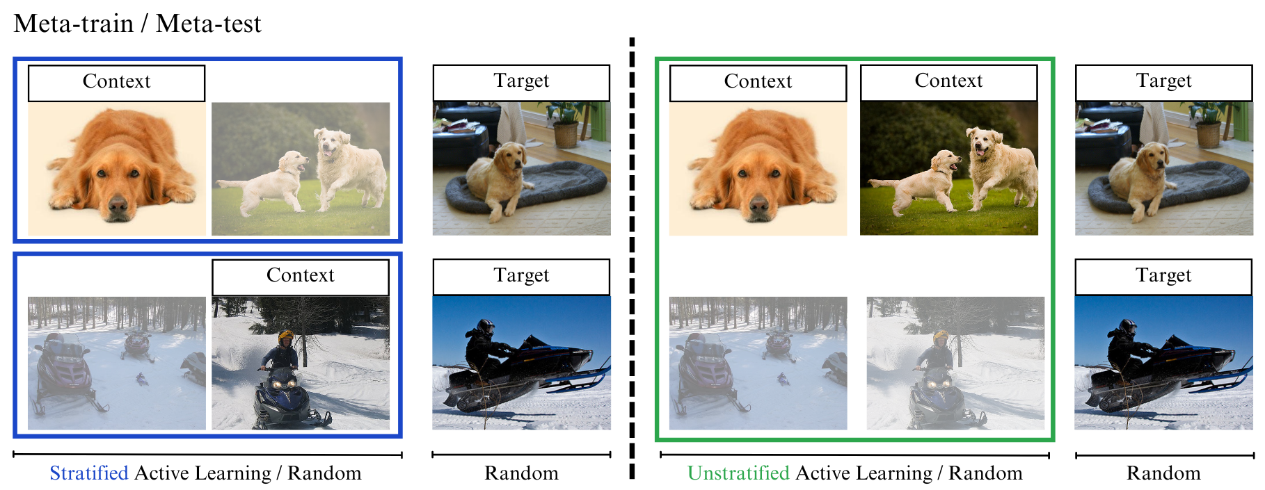
Figure 1: The meta-training process. $\operatorname{Pick}_{\theta}$ can be stratified or unstratified, active or passive.

Stratification

In passive few-shot classification, the $\operatorname{Pick}$ functions typically choose context points according to a stratified sample: for one-shot classification, $\mathcal{C}$ contains exactly one point per class. This is because, if we take a uniform random sample of size $N$ for an $N$-way classification problem, $\mathcal{C}$ is unlikely to contain all the classes, making classification very difficult. Assuming “nature” gives a stratified uniform sample, as in nearly all work on few-shot classification, also seems reasonable.

In pool-based active settings, however, it is highly unreasonable to assume that $\operatorname{Pick}_{\theta}^{\mathit{deploy}}$ can be stratified (as illustrated on the left side of Figure 1): to do so, we would need to know the label of every point in $\breve{\mathcal{D}}$, in which case we should simply use all those labels. As we would like $\operatorname{Pick}_{\theta}^{\mathit{eval}}=\operatorname{Pick}_{\theta}^{\mathit{deploy}}$, eval-time stratification is then not particularly reasonable; even so, we report such results per the standards of meta-learning. When $\operatorname{Pick}_{\theta}^{\mathit{deploy}}$ is unstratified (as in the right side of Figure 1), it is particularly important for the selection criterion to find samples from each class.

Train-time stratification with unstratified evaluation does not leak data labels, and is plausible when $\mathcal{P}^{\mathit{train}}$ and $\mathcal{P}^{\mathit{eval}}$ are fully labeled. Since this approach trains $f_{\theta}$ in an “easy” setting and evaluates it in a “hard” one, however, we will see it tends to slightly underperform the fully-unstratified default.

Regression problems are not typically stratified; we do not stratify for our regression experiments.

2.2 Related Work: Meta-Learning algorithms

Meta-learning algorithms can be divided into several categories; all will be applicable for our active learning strategies, and we evaluate with at least one representative algorithm per category.

Metric-based methods learn a representation space encoding a “good” similarity, where simple classifiers work well (Vinyals et al., 2016; Finn et al., 2018; Oreshkin et al., 2018). ProtoNet (Snell et al., 2017) finds features so that points from each class are close to the prototype feature of the class.

Optimization-based methods use $f_{\theta}$ that incorporate optimization, e.g. gradient descent as in MAML (Finn et al., 2017; Antoniou et al., 2019), which seeks parameters $\theta$ (especially a parameter initialization) such that gradient descent quickly finds a useful model on a new task. ANIL (Raghu et al., 2020) freezes most of the network and only updates the last layer, while R2D2 (Bertinetto et al., 2019) and MetaOptNet (Lee et al., 2019b) replace the last layer with a convex problem whose solution can be differentiated; these approaches can improve both performance and speed.

Model-based methods learn a model that explicitly adapts to new tasks, typically by modeling the distribution of $y$ from $\mathcal{T}$ given its $x$ values and $\mathcal{C}$. The most prominent family of methods is Neural Processes (NPs) (Garnelo et al., 2018b; Dubois et al., 2020), which encode a context set and estimate task-specific distribution parameters. Conditional (and latent) NPs can have issues with underfitting (Garnelo et al., 2018a; b), but AttentiveNPs (Kim et al., 2019) and ConvNPs (Gordon et al., 2020) can be more powerful. These models are more commonly used for regression.

Pre-training methods, such as SimpleShot (Wang et al., 2019) and Baseline++ (Chen et al., 2019), are based on repeated demonstrations (also Zhang et al., 2021; Goldblum et al., 2020) that simply pre-training a multi-class model can surpass the performance of commonly used meta-learners.

3 Active Learning

In pool-based active learning, a model requests labels for the most “informative” data points from a pool of unlabeled data. The key question is how to estimate which data points will be informative.

3.1 Related Work: Existing Active Learning Methods

Uncertainty-based methods

Simple but effective uncertainty-based methods such as maximum entropy (Wang & Shang, 2014), least confident (Settles, 2009), and margin sampling (Scheffer et al., 2001) are widely used for active learning. Since they only consider current models’ uncertainty, active learning strategies that consider expected changes in model parameters (Settles et al., 2007; Ash et al., 2020) and model outputs (Zhu et al., 2003; Guo & Greiner, 2007; Roy & McCallum, 2001; Käding et al., 2018; Freytag et al., 2014; Käding et al., 2016; Mohamadi et al., 2022) have been also been proposed. However, recent analyses have empirically demonstrated that at least in certain experimental settings, most active learning methods are not significantly different from one another (Lang et al., 2021), and may not even improve over random selection (Munjal et al., 2022).

Random

Uniformly randomly samples a context set from all the candidate data points.

Entropy

Add one point to the context set based on $x^{*}=\operatorname*{arg\,max}_{x\in\mathcal{U}}H(\hat{y}(x)\mid x)$, where $\mathcal{U}$ are the unlabeled candidate data points and $H(\cdot)$ is Shannon entropy (Wang & Shang, 2014). Other than in Appendix K, we apply this in “batch mode,”color=violet!20,noinline]Danica: update discussion i.e. we do not observe points one-by-one but rather choose the $\lvert\mathcal{C}\rvert$ points with the highest “initial” entropy.

Margin

For classification, add one point to $\mathcal{C}$ based on $x^{*}=\operatorname*{arg\,min}_{x\in\mathcal{U}}p_{1}(y|x)-p_{2}(y|x)$, where $p_{1}$ and $p_{2}$ denote the first and second highest predicted probabilities, respectively (Scheffer et al., 2001). We also run this method in “batch mode.”

Although Entropy and Margin are very simple and fast to evaluate, no uncertainty-based method seems to substantially outperform them on typical active image classification tasks (e.g. Mohamadi et al., 2022), and we will see that other methods are unlikely to be competitive in low-budget regimes.

Low-budget active learning

The limitations of typical active learning approaches may especially apply in very-low-budget cases, such as those considered in few-shot classification and meta-learning. In particular, when the “current” model is quite bad, using it to choose points might be counterproductive. In the one-shot case especially, standard active learning methods simply do not apply.

Recently, several papers have have proposed novel active learning algorithms for these settings; none of these papers focused on meta-learning, but should be broadly applicable since meta-learning is also a low-budget setting. Rather than picking e.g. the points about which a model is least certain, these papers propose to label the “most representative” data points independently of a “current” model.

DPP

Determinantal Point Processes (DPPs) can query diverse samples, based on selecting a subset that maximizes the determinant of a similarity matrix (Bıyık et al., 2019).

Typiclust

Run $k$-means on the unlabeled data points, where $k=\lvert\mathcal{C}\rvert$ is the annotation budget. Select one data point per cluster such that the distance between a data point and its $k^{\prime}$ nearest neighbors is minimized: $\operatorname*{arg\,min}_{x\in\mathcal{U}}\sum_{x^{\prime}\in\operatorname{NN}_{k^{\prime}}(x)}\lVert x-x^{\prime}\rVert_{2}$ (Hacohen et al., 2022).

Coreset

Greedily select a subset of the unlabeled data points to approximately minimize the distance from unlabeled data points to their nearest labeled point (Sener & Savarese, 2018).

ProbCover

Select data points that roughly maximize the number of unlabeled points within a distance of $\tau$ from any labeled point, where $\tau$ is chosen according to a “purity” heuristic (Yehuda et al., 2022); see Appendix F for more details.

3.2 Features for Representative-Selection Methods

Notions of the “most representative” data points are highly dependent on a reasonable metric of data similarity. Prior methods operated either on raw data – typically a poor choice for complex datasets like natural images – or, in semi-supervised settings as in ProbCover and Typiclust, on SimCLR (Chen et al., 2020) features learned on the unlabeled data.

In metric-based meta-learning, we propose to instead use the current meta-learned representation; choosing points representative for the features we will use downstream is the natural choice.

In MAML, the most natural equivalent might be features from the empirical neural tangent kernel (Lee et al., 2019a) of the current initialization network; this approximates what will happen when the network is trained on $\mathcal{C}$, and so is perhaps the best simple understanding of “how this network views the data.” Even empirical NTKs are often expensive to evaluate, however, and we thus propose to instead use features from the penultimate layer of the initialization neural net $f_{\theta}(\{\})$, corresponding to the NTK of a model that only retrains its last layer (as in ANIL, R2D2, and MetaOptNet).

We also use the penultimate-layer reperesentations of $f_{\theta}(\{\})$ for NP-based meta-learning.

Experiments in Appendix I show that this proposal outperforms separate self-supervised features.

3.3 Gaussian Mixture Selection for Low-Budget Active Learning

We propose the following very simple algorithm for low-budget active learning: fit a mixture of $k$ Gaussians to the unlabeled data features, where $k$ is the label budget, using EM with a $k$-means initialization. We use a shared diagonal covariance matrix. Once a mixture is fit, we select the highest-density point from each component: $\operatorname*{arg\,min}_{x\in\mathcal{U}}(x-\mu_{j})^{\mathsf{T}}\Sigma^{-1}(x-\mu_{j})$ for each $j\in[k]$.

For metric-based meta-learning, the motivation of this algorithm is clear: we want labeled points that approximately “cover” the data points. Our notion of a “cover” is somewhat different from that of Coreset (Sener & Savarese, 2018) or ProbCover (Yehuda et al., 2022); we avoid ProbCover’s need for a fixed radius, which we show can lead to poor choices (see Appendix F), and are more concerned with “average” covering (and hence perhaps less sensitive to outliers) than Coreset. The quality of selected data points from those methods are compared according to a few metrics in Figure 6.

On ANIL and MetaOptNet: since $\lvert\mathcal{C}\rvert$ is at most, say, 50 (in $10$-way $5$-shot) and the feature dimension is typically hundreds, ANIL becomes approximately the same multiclass max-margin separator obtained by (unregularized) MetaOptNet. Intuitively, as $\lvert\mathcal{C}\rvert$ grows, the means of an isotropic Gaussian mixture converge to roughly a covering set for the dataset $\mathcal{U}$, and the max-margin separator of a set cover for $\mathcal{U}$ will be similar to the max-margin separator for all of the data. Even in various cases when $\lvert\mathcal{C}\rvert\ll\lvert\mathcal{U}\rvert$, choosing the means yields a max-margin separator that generalizes well.

Figure 4 in Appendix A illustrates that, if class-conditional data distributions are isotropic Gaussians with the same covariance matrices, labeling the cluster centers can be far preferable to labeling a random point from each cluster. This is backed up by the following result in a particular simple case:

propositionpropname Suppose $Y\sim\mathrm{Uniform}([N])$, and $X\mid Y=y\sim\mathcal{N}(\mu_{y},\sigma^{2}I)$, where the $\mu_{i}$ are orthonormal. Then the max-margin separator (4) on $\{(\mu_{i},i)\}_{i=1}^{N}$ is Bayes-optimal for $Y\mid X=x$.

For more general settings, we argue that GMM is still a good method based on being an efficient set cover, as shown in Figure 5 in Appendix A along with the proof for Section 3.3.

Very-low-budget regime

Active learning based on Gaussian mixtures is not new in itself. Closely-related methods such as $k$-means, $k$-means⁺⁺ or $k$-medoids have been used as sole selection algorithms (Aghaee et al., 2016; Voevodski et al., 2012) or in combination with uncertainty-based methods (Nguyen & Smeulders, 2004; Donmez et al., 2007; Ash et al., 2020; Hacohen et al., 2022). Some recent work (Boney & Ilin, 2017) including DPP (Bıyık et al., 2019) and Coreset (Sener & Savarese, 2018) show significant improvements over GMM-based baselines. These trends, however, do not seem to hold true in very-low-budget regimes such as meta-learning. As shown in Figure 2, GMM matches or outperforms other low-budget methods with very small numbers of labels for standard image classification tasks; the following section shows that GMM provides substantial improvements in meta-learning.

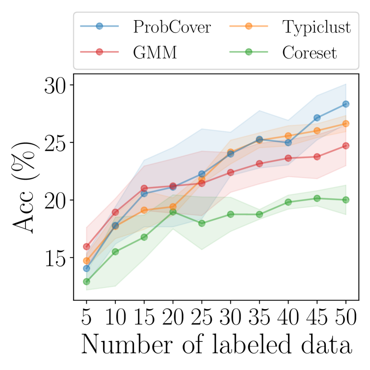
(a) CIFAR10

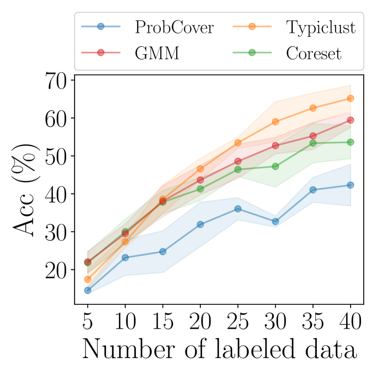
(b) MNIST

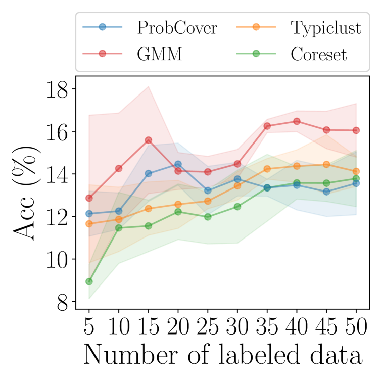
(c) SVHN

Figure 2: Low-budget active learning methods on supervised image classification with very low budget. Mean and standard error for three sets of SimCLR features, three runs per features.

4 Active Meta-Learning Experiments

We now compare various active learning methods for variants of active meta learning as defined in Section 2.1, on both classification tasks (in Sections 4.1 and 4.2) and regression (in Section 4.3). color=blue!30,]Won: add the problem of sequential active meta

4.1 Few-shot Image Classification

We use four popular few-shot image classification benchmark datasets. MiniImageNet (Vinyals et al., 2016; Ravi & Larochelle, 2017) consists of $60\,000$ images sampled from ImageNet (Deng et al., 2009), with $64$ train classes, $16$ validation, and $20$ test. Each class has $600$ images. TieredImageNet (Ren et al., 2018) is a much larger subset of ImageNet; it consists of $34$ super-classes, each containing $10$ to $30$ sub-classes. There are $20$ train super-classes, $6$ validation, and $8$ test. FC100 (Oreshkin et al., 2018) is a subset of CIFAR100 (Krizhevsky, 2009), with $60$ train classes, $20$ validation, and $20$ test. It is designed to minimize the overlap between the splits. CUB (Wah et al., 2011; Hilliard et al., 2018) consists of $200$ classes of bird images, with $140$ train classes, $30$ validation, and $30$ test.

We validate whether our active learning methods work across various types of meta-learning algorithms. We run metric-based: ProtoNet (Snell et al., 2017), optimization-based: MAML (Finn et al., 2017), ANIL (Raghu et al., 2020), and MetaOpt(Lee et al., 2019b), as well as pre-training-based: Baseline++ (Chen et al., 2019) and SimpleShot (Wang et al., 2019).We vary the backbone to demonstrate robustness: for instance, we use 4 convolutional blocks for MAML and ProtoNet, and ResNet10 (He et al., 2016) for Baseline++. As typical in few-shot classification, we report means and 95% confidence intervals for test accuracy from a single model, based on 600 meta-test samples.

We use the meta-learner’s features as proposed in Section 3.2 for all methods; experiments in Appendix I confirm that they outperform contrastive learning of features on the meta-training set. Additionally, in the main body we only present results where $\operatorname{Pick}_{\theta}^{\mathit{train}}$ is random; Appendix J demonstrates that, in our setup, active learning at train time is actually mildly harmful to overall performance, which aligns with the observations in Ni et al. (2021) and Setlur et al. (2020).

For metric-based methods, Table 1 shows results for ProtoNet on FC100. The simple GMM method significantly outperforms the other active learning strategies on all problem variants considered here. As previously reported (Hacohen et al., 2022; Yehuda et al., 2022), uncertainty-based methods are significantly worse than random selection in this low-budget regime.

For optimization-based, Table 2 shows results with MAML on MiniImageNet. Similar to Table 1, GMM again significantly outperforms the other strategies in most cases. The performance of ProbCover is sometimes much lower than other methods due to its radius parameter, which is very difficult to tune, with the best choice changing dramatically depending on the sub-task even though Yehuda et al. (2022) proposed to fix this parameter per dataset (see Appendix F for more). Results for ANIL on TieredImageNet and MetaOptNet on FC100 are provided in Appendix G.

For pre-training-based methods, we compare active learning strategies with Baseline++ on the CUB dataset in Table 3, seeing that the proposed method is again usually by far the best, though in one five-shot case it essentially ties DPP. As these methods do not follow the meta-training process in (1), train-time stratification is not applicable. Appendix G shows results for SimpleShot.

$\operatorname{Pick}_{\theta}^{\mathit{eval}}$	1-Shot			5-Shot
	Fully strat.	Train strat.	Unstrat.	Fully strat.	Train strat.	Unstrat.
Random	$36.73\pm 0.18$	$31.27\pm 0.21$	$31.40\pm 0.41$	$47.98\pm 0.18$	$42.83\pm 0.20$	$44.00\pm 0.21$
Entropy	$33.67\pm 0.16$	$29.82\pm 0.20$	$30.01\pm 0.20$	$44.64\pm 0.17$	$38.39\pm 0.22$	$38.36\pm 0.25$
Margin	$34.28\pm 0.18$	$29.74\pm 0.20$	$28.99\pm 0.20$	$45.31\pm 0.17$	$39.65\pm 0.21$	$38.13\pm 0.24$
DPP	$36.20\pm 0.18$	$31.34\pm 0.20$	$31.09\pm 0.20$	$47.53\pm 0.17$	$43.69\pm 0.20$	$44.19\pm 0.20$
Coreset	$35.79\pm 0.17$	$30.31\pm 0.20$	$31.57\pm 0.18$	$43.08\pm 0.40$	$41.56\pm 0.20$	$41.79\pm 0.22$
Typiclust	$46.01\pm 0.16$	$30.96\pm 0.19$	$30.61\pm 0.21$	$47.54\pm 0.17$	$43.61\pm 0.18$	$44.03\pm 0.21$
ProbCover	$48.66\pm 0.16$	$32.86\pm 0.22$	$33.58\pm 0.19$	$51.11\pm 0.17$	$44.20\pm 0.23$	$44.40\pm 0.24$
GMM (Ours)	$50.22\pm 0.18$	$34.23\pm 0.23$	$35.03\pm 0.23$	$54.76\pm 0.17$	$46.30\pm 0.21$	$47.03\pm 0.20$

Table 1: 5-Way K-Shot classification on FC100 with ProtoNet, with $\operatorname{Pick}_{\theta}^{\mathit{train}}$ random. The first, second, third best results for each setting are marked in this and all other results tables.

$\operatorname{Pick}_{\theta}^{\mathit{eval}}$	1-Shot			5-Shot
	Fully strat.	Train strat.	Unstrat.	Fully strat.	Train strat.	Unstrat.
Random	$47.93\pm 0.20$	$28.16\pm 0.17$	$34.85\pm 0.19$	$64.16\pm 0.18$	$53.54\pm 0.20$	$58.84\pm 0.20$
Entropy	$48.16\pm 0.20$	$25.56\pm 0.14$	$30.44\pm 0.17$	$61.22\pm 0.20$	$34.36\pm 0.23$	$39.57\pm 0.26$
Margin	$48.31\pm 0.20$	$28.32\pm 0.16$	$30.83\pm 0.17$	$63.73\pm 0.18$	$49.24\pm 0.22$	$53.92\pm 0.22$
DPP	$48.96\pm 0.21$	$28.90\pm 0.17$	$36.44\pm 0.19$	$64.15\pm 0.18$	$54.18\pm 0.20$	$57.86\pm 0.19$
Coreset	$47.74\pm 0.20$	$29.19\pm 0.18$	$33.71\pm 0.18$	$61.28\pm 0.18$	$30.98\pm 0.19$	$45.74\pm 0.23$
Typiclust	$55.65\pm 0.18$	$27.45\pm 0.17$	$35.46\pm 0.18$	$64.16\pm 0.18$	$46.70\pm 0.21$	$57.83\pm 0.21$
ProbCover	$52.07\pm 0.17$	$23.34\pm 0.11$	$37.29\pm 0.18$	$64.66\pm 0.18$	$40.01\pm 0.21$	$45.32\pm 0.22$
GMM (Ours)	$58.82\pm 0.24$	$33.34\pm 0.24$	$37.68\pm 0.19$	$67.18\pm 0.18$	$54.35\pm 0.20$	$59.05\pm 0.20$

Table 2: 5-Way K-Shot classification on MiniImageNet with MAML, with $\operatorname{Pick}_{\theta}^{\mathit{train}}$ random.

Comparison between active learning methods.

Figure 3 (left) visualizes context set selection using t-SNE (van der Maaten & Hinton, 2008) for one 5-way, 1-shot, unstratified task. It is vital to select one sample from each class; only GMM does so here. Figure 3 (right) summarizes behavior across many tasks; while not perfect, GMM does a much better job of selecting distinct classes.

Entropy and Margin are typically far worse than random. So is Coreset, agreeing with prior observations (Ash et al., 2020; Hacohen et al., 2022; Yehuda et al., 2022); this may be because of issues with the greedy algorithm and/or sensitivity to outliers. Typiclust tends to pick points which, while dense according to its “typicality measure,” are far from cluster centers; this may be helpful in traditional active learning, but seems to hurt here. DPP is often better than random, but only barely; diverse selections may not necessarily lead to representative selections.

ProbCover manages to cover the feature space well, and is usually second-best. However, its “hard” radius causes issues; it may be preferable to use a smoother notion, as in GMM. The “purity” heuristic to choose a radius $\delta$ also does not seem to align well with model performance for meta-learning, as shown in Appendix F.

GMM, by contrast, provides robust performance without introducing significant new hyperpameters.

“Soft” $k$-means would be a special case of GMM with a spherical covariance. For some cases, standard $k$-means performs about the same as the GMM, but the GMM is occasionally much better: for Baseline++ on CUB, GMM outperforms $k$-means by $3.95$ points for 5-way 1-shot and $11.79$ for 5-shot. We provide a more thorough comparison to $k$-means in Appendix E.

$\operatorname{Pick}_{\theta}^{\mathit{eval}}$	1-Shot		5-Shot
	Test strat.	Test unstrat.	Test strat.	Test unstrat.
Random	$68.44\pm 0.92$	$51.03\pm 0.88$	$82.66\pm 0.56$	79.57 $\pm$ 0.67
Entropy	$66.33\pm 0.91$	$45.31\pm 0.89$	$80.97\pm 0.60$	$78.33\pm 0.72$
Margin	$68.65\pm 0.90$	$50.48\pm 0.94$	82.29 $\pm$ 0.64	$71.07\pm 0.83$
DPP	71.53 $\pm$ 0.89	$54.38\pm 0.92$	82.81 $\pm$ 0.55	78.62 $\pm$ 0.76
Coreset	$69.01\pm 0.91$	56.22 $\pm$ 0.94	$82.07\pm 0.55$	$76.35\pm 0.74$
Typiclust	$70.58\pm 0.81$	$29.80\pm 0.32$	$74.86\pm 0.81$	$70.00\pm 0.92$
ProbCover	78.11 $\pm$ 0.69	55.09 $\pm$ 0.98	$78.59\pm 0.64$	$65.71\pm 0.97$
GMM (Ours)	79.98 $\pm$ 0.60	59.55 $\pm$ 0.87	82.55 $\pm$ 0.58	82.68 $\pm$ 0.57

Table 3: 5-Way K-Shot classification on CUB with Baseline++, with $\operatorname{Pick}_{\theta}^{\mathit{train}}$ random.

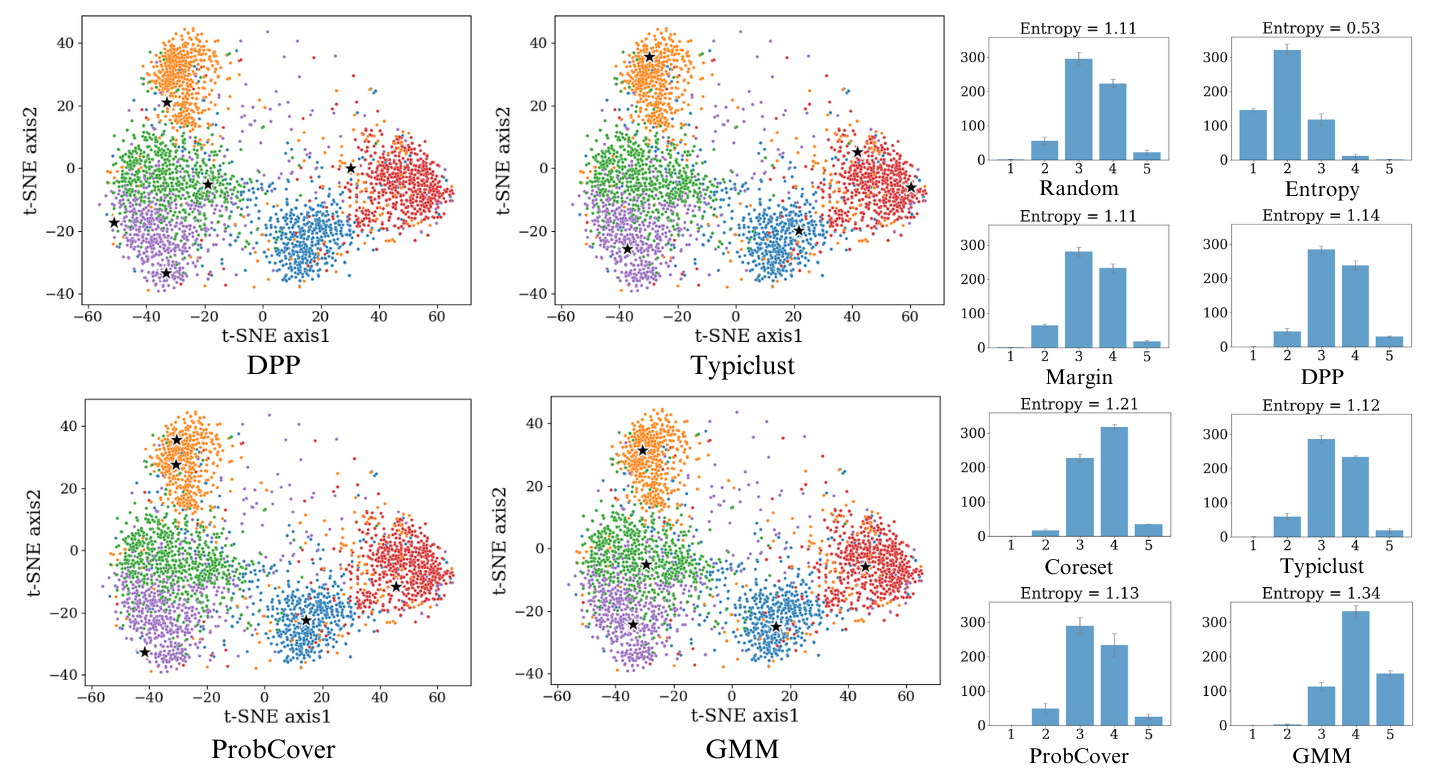
Figure 3: Left. t-SNE visualization of unlabeled points of one 5-way, 1-shot, unstratified MiniImageNet task. Stars denote selected context points using each method. Right. Distributions of the number of classes selected in each $\widetilde{\mathcal{C}}$ by ProtoNet on MiniImageNet among 600 meta-test cases, along with the mean empirical entropy of $y$ from $\widetilde{\mathcal{C}}$. The higher the value is, the more diverse classes an active learning method selects; $\log 5\approx 1.6$ would be perfect.

4.2 Cross-Domain Active Meta-Learning

Cross-domain learning, where $\mathcal{P}^{\mathit{train}}$ is “fundamentally different” from $\mathcal{P}^{\mathit{eval}}$, is typically more difficult than “in-domain" meta-learning. We use a ResNet18 (He et al., 2016) pretrained with standard supervised learning on ImageNet, and meta-test on CUB and Places (Zhou et al., 2017), which contains images of “places” such as restaurants and phone booths. As used for cross-domain meta-learning by Oh et al. (2022), it contains $16$ classes with an average of $1{,}715$ images each. As the model is not meta-trained, train stratification is not relevant; we show results in Table 4 only for unstratified test sets. The GMM method is again the clear overall winner; all other methods are often worse than random.

$\operatorname{Pick}_{\theta}^{\mathit{eval}}$	$P^{\mathit{eval}}$ on Places		$P^{\mathit{eval}}$ on CUB
	1-Shot	5-Shot	1-Shot	5-Shot
Random	$44.28\pm 1.93$	$77.92\pm 1.70$	$49.93\pm 0.92$	84.38 $\pm$ 0.72
Entropy	$36.12\pm 1.25$	$57.79\pm 2.93$	$41.85\pm 0.99$	$71.15\pm 0.99$
Margin	$43.31\pm 1.97$	$73.65\pm 1.94$	$48.04\pm 0.98$	$78.84\pm 0.92$
DPP	$46.76\pm 2.29$	78.36 $\pm$ 1.89	51.41 $\pm$ 0.90	84.19 $\pm$ 0.72
Coreset	50.03 $\pm$ 0.93	$65.20\pm 2.77$	$50.77\pm 0.95$	$81.80\pm 0.81$
Typiclust	$43.76\pm 1.98$	77.57 $\pm$ 1.84	$43.39\pm 1.03$	$50.69\pm 1.08$
ProbCover	47.93 $\pm$ 1.08	$59.08\pm 2.50$	62.13 $\pm$ 1.08	$69.80\pm 1.16$
GMM (Ours)	60.01 $\pm$ 0.86	86.45 $\pm$ 1.42	59.87 $\pm$ 0.86	85.49 $\pm$ 0.67

Table 4: Cross-domain meta-learning tasks using a ResNet18 pre-trained on ImageNet.

4.3 Active Meta-Learning for Regression

Each sinusoidal function (Finn et al., 2017) has task $y=a\sin(x+p)$, where $a\sim\text{Unif}(0.1,5)$ is the amplitude, and $p\sim\text{Unif}(0,\pi)$ is the phase of sine functions; we use MAML for this dataset.

Distractor and ShapeNet1D are vision regression datasets (Gao et al., 2022); the task is to predict the position of a specific object in an image ignoring a distractor, or to predict an object’s 1D pose (azimuth rotation). IC uses objects whose classes were observed during meta-training, while CC has novel object classes. We use conditional Neural Processes (NP) for Distractor, and attentive NP for ShapeNet1D. Details are provided in Appendix H.

Table 5 compares active strategies on these datasets; GMM again performs generally the best.

Active Strategy	Sine func. (3-Shots)	Distractor (2-Shots)		ShapeNet1D (2-Shots)
		IC	CC	IC	CC
Random	$24.17\pm 0.43$	$18.91\pm 2.13$	$25.79\pm 2.17$	$16.52\pm 1.08$	$19.07\pm 1.30$
DPP	23.19 $\pm$ 0.51	18.08 $\pm$ 2.12	19.68 $\pm$ 1.92	11.83 $\pm$ 0.85	13.68 $\pm$ 0.93
Coreset	$31.36\pm 0.48$	19.58 $\pm$ 1.95	24.08 $\pm$ 2.19	11.39 $\pm$ 0.91	13.05 $\pm$ 1.18
Typiclust	21.59 $\pm$ 0.40	$20.27\pm 2.15$	$24.96\pm 2.68$	$12.54\pm 1.08$	$14.58\pm 1.24$
ProbCover	$29.36\pm 0.49$	$21.96\pm 2.45$	$25.25\pm 2.78$	$12.31\pm 0.85$	$13.95\pm 1.08$
GMM (Ours)	18.09 $\pm$ 0.38	17.95 $\pm$ 2.05	22.03 $\pm$ 2.42	10.78 $\pm$ 0.72	12.35 $\pm$ 0.97

Table 5: Meta-learning for regression on a toy dataset and two pose estimation datasets for Intra-Category (IC) and Cross-Category (CC). Sine func. and Distractor use mean squared error, ShapeNet1D uses cosine-sine-distance; lower values are better for each.

5 Discussion

We have clarified the ways in which active learning can be incorporated into meta-learning. While active context set selection does not seem to work at meta-training time (Appendix J), it can be extremely useful at meta-testing/deployment time.

We proposed a surprisingly simple method that substantially outperforms previous proposals. It is simple and intuitive, and bears some theoretical guarantees in a particular simple situation, though why it improves so thoroughly over related methods is not yet fully clear.

While we evaluated on a range of methods across many datasets, we focused on convolutional models for computer vision tasks; although we see no particular reason to expect this, it’s conceivable that things might behave differently with other types of data and/or models.

Reproducibility

For each experiment, we listed implementation details of the experiment such as model, optimizer, batch size, and training iterations, along with the links to publicly available code we built on, in Appendix B. Anonymous code is provided in the supplementary material. For the theoretical result, we clearly mentioned conditions and provided a complete proof in Appendix A.

Acknowledgements

This work was supported in part by the Natural Sciences and Engineering Resource Council of Canada, the Canada CIFAR AI Chairs program, the BC DRI Group, Compute Ontario, and the Digital Resource Alliance of Canada.

Appendix A Details for Max-Margin Motivation

The following optimization problem is one form of an $N$-class max-margin problem, i.e. a multi-class support vector machine (Crammer & Singer, 2001), on a training set $\{(x_{i},y_{i})\}_{i=1}^{m}$:

$$\min_{w_{1},\dots,w_{N}}\sum_{y=1}^{N}\lVert w_{y}\rVert^{2}\;\text{ s.t. }\;\forall i\in[m],\;\forall y^{\prime}\neq y_{i},\;w_{y_{i}}^{\mathsf{T}}x_{i}\geq w_{y^{\prime}}^{\mathsf{T}}x_{i}+1.$$ (4)

This is a “hard” version of the problem used as a classification head by MetaOptNet (Lee et al., 2019b), and can be obtained in their framework by taking the penalty parameter $C\to\infty$.

and can be obtained in their framework by taking the penalty parameter $C\to\infty$.

The decision boundaries obtained by small-step-size gradient descent for linear predictors with cross-entropy loss on separable data converge to those obtained by (4), as shown by Soudry et al. (2018, Theorem 7), for almost all datasets. Thus, ANIL (Raghu et al., 2020), which uses gradient descent for linear predictors with cross-entropy loss on separable data, will approximately obtain the same solution when using enough steps with appropriately small learning rates.

MetaOptNet uses the homogeneous predictors discussed here. We can handle non-homogeneous linear predictors ($w^{\mathsf{T}}x+b$ instead of just $w^{\mathsf{T}}x$) with the standard trick of adding a constant $1$ feature to each data point. This solution actually does not quite maximize the margin on the original problem, since it effectively adds $b^{2}$ to the objective in (4), but ANIL will find exactly this same solution when using gradient descent on a function with a separate intercept term.

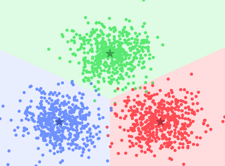
(a) Trained on cluster centers

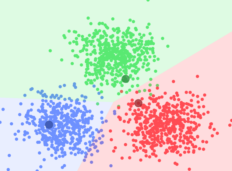
(b) Trained on random points

Figure 4: Decision boundaries using a multiclass SVM (4) trained on a one-shot dataset containing (a) cluster centers (shown by stars) and (b) randomly selected points (shown by circles).

Figure 4 demonstrates visually that, if the class-conditional data distributions are isotropic Gaussians with the same covariance matrices, labeling the cluster centers can be far preferable to labeling a random point from each cluster. This is backed up by the following result in a particular case: *

Proof.

Combine Lemmas 1 and 2 below. ∎

The orthonormal assumption keeps the proof tractable; far more analysis would be needed without it. With high-dimensional meta-learned features that are well-aligned to the learning problem, however, it is reasonable to expect that inner products between different classes will be much smaller than the within-class inner products.

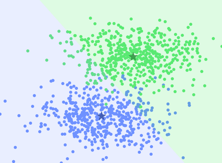
(a) Trained on $N$ cluster centers

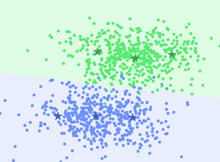
(b) Trained on $3N$ cluster centers

Figure 5: Decision boundaries using a multiclass SVM (4) trained on cluster centers (shown by stars), with (a) the one-shot case and (b) the three-shot case.

This optimality result can break when the clusters do not share a spherical covariance; consider Figure 5(a), where the data is still Gaussian but the shared class-conditional covariance is not spherical. In the one-shot case, max-margin on the separators does not choose the optimal separator. In this case, we could manually select points to choose the correct line. Doing so, however, is quite risky; since we do not know the data labels (or that it is actually Gaussian), we might incorrectly separate the data. Figure 5(b) shows the same problem in a three-shot setting; here, even though the data is truly generated from a mixture of two Gaussians, fitting a mixture of six Gaussians gives us an approximate set cover of the data, and the max-margin separator now works well.

In fact, we can expect that (a) as the number of clusters grows, the cluster centers produce a better and better set cover of the dataset; (b) the max-margin separator on a set cover will approximate the max-margin separator on the full dataset, since the support vectors are all nearby. color=violet!20,noinline]Danica: would be nice to prove this…sigh

A.1 Proofs

Lemma 1.

Suppose that $\{x_{i}\}_{i=1}^{N}$ are orthonormal. Then the solution to (4) with the dataset $\{(x_{y},y)\}_{y=1}^{N}$ is given by $w_{y}=x_{y}-\frac{1}{N}\sum_{i=1}^{N}x_{i}$, and hence

$$\operatorname*{arg\,max}_{y}w_{y}^{\mathsf{T}}x=\operatorname*{arg\,min}_{y}\lVert x-x_{y}\rVert.$$

Proof.

We will be able to analytically solve the KKT conditions for (4) in this case. Rather than using existing analyses of (4), it will be simpler to directly analyze this particular case.

Let $\mathbf{w}=\begin{bmatrix}w_{1}\\ \vdots\\ w_{N}\end{bmatrix}\in\mathbb{R}^{Nd}$, where $d$ is the dimension of the $x_{i}$ and $w_{y}$. The objective of our optimization problem is then simply $\lVert\mathbf{w}\rVert^{2}$.

We will next define a matrix $A$ such that the constraints can be written as $A\mathbf{w}+\mathbf{1}\leq\mathbf{0}$, with $A\in\mathbb{R}^{N(N-1)\times Nd}$ and $\leq$ interpreted elementwise. Each constraint is of the form $-w_{i}^{\mathsf{T}}x_{i}+w_{j}^{\mathsf{T}}x_{i}+1\leq 0$, where $i\neq j$ are class indices in $[N]$. We can write the corresponding row of $A$ as $(E_{j}-E_{i})x_{i}$, where $E_{i}\in\mathbb{R}^{Nd\times d}$ are given by $E_{i}=\begin{bmatrix}0_{(i-1)d\times d}\\ I_{d}\\ 0_{(N-i-1)d\times d}\end{bmatrix}$; these $E_{i}$ are a block-matrix analogue of standard basis vectors, so that $E_{i}x_{i}\in\mathbb{R}^{Nd}$ has $x_{i}$ in the $i$th block of $d$ coordinates, and $0$ elsewhere. We will order these constraints in $A$ in “row-major” order: recalling that $i\neq j$, this means we have first $i=1\;j=2$, then $i=1\;j=3$, up to $i=1\;j=N$, followed by $i=2\;j=1$, $i=2\;j=3$, and so on. Let $\ell(i,j)$ give the index of the corresponding constraint, so that e.g. $\ell(1,3)=2$.

Now, the problem can be written

$$\min_{\mathbf{w}\in\mathbb{R}^{Nd}}\frac{1}{2}\lVert\mathbf{w}\rVert^{2}\;\text{s.t.}\;A\mathbf{w}+\mathbf{1}\leq\mathbf{0},$$

with the $\frac{1}{2}$ introduced for convenience. The KKT conditions for this problem are

$$\mathbf{w}+A^{\mathsf{T}}\mu=\mathbf{0}\quad A\mathbf{w}+\mathbf{1}\leq\mathbf{0}\quad\mu\geq\mathbf{0}\quad\mu\odot(A\mathbf{w}+\mathbf{1})=\mathbf{0},$$

where $\odot$ is elementwise multiplication. From the first condition, $\mathbf{w}=-A^{\mathsf{T}}\mu$, where $\mu\in\mathbb{R}^{N(N-1)}$ is any vector satisfying

$$\mu\geq\mathbf{0}\quad AA^{\mathsf{T}}\mu-\mathbf{1}\geq\mathbf{0}\quad\mu\odot(AA^{\mathsf{T}}\mu-\mathbf{1})=\mathbf{0}.$$

Since (4) is a strictly convex minimization problem with affine constraints, these conditions are necessary and sufficient for optimality, and the solution $\mathbf{w}$ is unique.

We can reasonably expect, since the $x_{i}$ are orthonormal, that all constraints should be active, meaning that $AA^{\mathsf{T}}\mu=\mathbf{1}$. Indeed, choosing $\mu=(AA^{\mathsf{T}})^{-1}\mathbf{1}$ automatically satisfies the second and third conditions; it only remains to show that this $\mu\geq\mathbf{0}$ in order to show this as an optimal solution to (4).

To do this, we will explicitly characterize $AA^{\mathsf{T}}$:

$$(AA^{\mathsf{T}})_{\ell(i,j),\ell(i^{\prime},j^{\prime})}=x_{i}^{\mathsf{T}}(E_{j}-E_{i})^{\mathsf{T}}(E_{j^{\prime}}-E_{i^{\prime}})x_{i^{\prime}}=(\delta_{ii^{\prime}}+\delta_{jj^{\prime}}-\delta_{ij^{\prime}}-\delta_{ji^{\prime}})\,x_{i}^{\mathsf{T}}x_{i^{\prime}},$$

where $\delta_{ij}=\mathds{1}(i=j)$ is the Kronecker delta, since $E_{i}^{\mathsf{T}}E_{j}=\delta_{ij}I_{d}$.

Since the $x_{i}$ are orthonormal, $x_{i}^{\mathsf{T}}x_{i^{\prime}}=\delta_{ii^{\prime}}$. As we know $i\neq j$ and $i^{\prime}\neq j^{\prime}$, this simplifies to

$$(AA^{\mathsf{T}})_{\ell(i,j),\ell(i^{\prime},j^{\prime})}=\delta_{ii^{\prime}}(1+\delta_{jj^{\prime}}).$$

Thus $(AA^{\mathsf{T}})$ is a block matrix with diagonal blocks of size $(N-1)\times(N-1)$ with values $I_{N-1}+\mathbf{1}_{N-1}\mathbf{1}_{N-1}^{\mathsf{T}}$, and all off-diagonal blocks zero. Taking $\mu=(AA^{\mathsf{T}})^{-1}\mathbf{1}_{N(N-1)}$, the zero blocks contribute nothing, so each block of $N-1$ entries of $\mu$ is $(I_{N-1}+\mathbf{1}_{N-1}\mathbf{1}_{N-1})^{-1}\mathbf{1}_{N-1}$.

Note that $\mathbf{1}_{N-1}\mathbf{1}_{N-1}^{\mathsf{T}}$ has one eigenvector $v_{1}=\frac{1}{\sqrt{N-1}}\mathbf{1}$ with eigenvalue $\lambda_{1}=N-1$, and the remaining eigenvalues are all zero with eigenvectors satisfying $v_{i}^{\mathsf{T}}\mathbf{1}=0$. Adding $I$ to this matrix simply increases all eigenvalues by one. Thus

$$\left(I+\mathbf{1}\mathbf{1}^{\mathsf{T}}\right)^{-1}\mathbf{1}=\frac{1}{N}\left(\frac{1}{\sqrt{N-1}}\mathbf{1}\right)\left(\frac{1}{\sqrt{N-1}}\mathbf{1}\right)^{\mathsf{T}}\mathbf{1}+\sum_{i=2}^{N-1}v_{i}\underbrace{v_{i}^{\mathsf{T}}\mathbf{1}}_{0}=\frac{1}{N}\underbrace{\frac{\mathbf{1}^{\mathsf{T}}\mathbf{1}}{N-1}}_{1}\mathbf{1}=\frac{1}{N}\mathbf{1},$$

and so $\mu=\frac{1}{N}\mathbf{1}_{N(N-1)}$, which is indeed $\geq\mathbf{0}$; thus this is an optimal solution to the problem.

We next reconstruct $\mathbf{w}=-A^{\mathsf{T}}\mu=-\frac{1}{N}A^{\mathsf{T}}\mathbf{1}_{N(N-1)}$. Consider the block $w_{i}$ inside $\mathbf{w}$; its value will be the negative mean of the entries of $A$ with an $E_{i}$ in them. The $\ell(i,j)$ rows for $j\neq i$ contribute $N-1$ entries of the form $-E_{i}x_{i}$. We also have the $\ell(k,i)$ rows, which have one $E_{i}x_{k}$ term for each $k\neq i$. Thus

$$w_{i}=-\frac{1}{N}\left(-(N-1)x_{i}+\sum_{k\neq i}x_{k}\right)=-\frac{1}{N}\left(-Nx_{i}+\sum_{k=1}^{N}x_{k}\right)=x_{i}-\bar{x},$$

where $\bar{x}=\frac{1}{N}\sum_{k=1}^{N}x_{k}$. Thus, for a test point $x$,

$$\operatorname*{arg\,max}_{i}w_{i}^{\mathsf{T}}x=\operatorname*{arg\,max}_{i}x_{i}^{\mathsf{T}}x-\bar{x}^{\mathsf{T}}x=\operatorname*{arg\,max}_{i}x_{i}^{\mathsf{T}}x.$$

Because the $x_{i}$ are orthonormal, this is further equal to

$$\operatorname*{arg\,min}_{i}\lVert x_{i}\rVert^{2}+\lVert x\rVert^{2}-2x_{i}^{\mathsf{T}}x=\operatorname*{arg\,min}_{i}\lVert x-x_{i}\rVert.\qed$$

Lemma 2.

If $X\mid Y=y\sim\mathcal{N}(\mu_{y},\sigma^{2}I)$ and $Y\sim\operatorname{Uniform}([N])$, the Bayes-optimal classifier is given by

$$f^{*}(x)=\operatorname*{arg\,min}_{y}\lVert x-\mu_{y}\rVert.$$

Proof.

This well-known fact follows by combining

$$p(Y=y\mid X=x)=\frac{p(X=x\mid Y=y)p(Y=y)}{p(X=x)}\propto p(X=x\mid Y=y)$$

with the definition of the density for $X$,

$$\operatorname*{arg\,max}_{y}\frac{1}{(2\pi\sigma^{2})^{d/2}}\exp\left(-\frac{1}{2\sigma^{2}}\lVert x-\mu_{y}\rVert^{2}\right)=\operatorname*{arg\,min}_{y}\lVert x-\mu_{y}\rVert.\qed$$

Appendix B Implementation Details for Meta Learning Algorithms

Metric-based

We use a meta learning library called learn2learn (Arnold et al., 2020) to implement ProtoNet (Snell et al., 2017). Following the original paper, we train a model with $30$-way and $20$-way for 1-Shot and 5-Shot, respectively, for $3{,}000$ iterations. We use a 4 layer convolutional neural network (Conv4) with $64$ channel size, and the batch size is set to $100$. For optimization, we employ an Adam optimizer with a learning rate of $0.01$ without having a learning rate schedule.

Optimization-based

We use the learn2learn library to implement both MAML (Finn et al., 2017) and ANIL (Raghu et al., 2020). We use Conv4 with $32$ channel size for MAML and $64$ channel size for ANIL (larger channel size does not perform better for MAML). We train both MAML and ANIL for $60{,}000$ iterations. For optimizer, we employ an Adam optimizer for both with learning rates of $0.003$ and $0.001$ (adaptation learning rates of $0.5$ and $0.1$) for MAML and ANIL, respectively. Batch sizes are set to $32$ for both.

For MetaOptNet (Lee et al., 2019b), we use the publicly available code provided by the authors of the paper (https://github.com/kjunelee/MetaOptNet). We employ the dual formulation of Support Vector Machine (SVM) proposed in MetaOptNet (MetaOptNet-SVM) for experiments with the training shot of $15$, and use the default hyperparameter settings. For instance, we use a SGD optimizer with initial learning rate of $0.1$ which decays step-wise. We train a model for $60$ epochs with a batch size of $8$.

Model-based

For both Conditional Neural Process (CNP) (Garnelo et al., 2018a) and Attentive Neural Process (ANP) (Kim et al., 2019), we use the publicly available code provided by the authors of the paper that addresses regression tasks for computer vision problems (Gao et al., 2022) (https://github.com/boschresearch/what-matters-for-meta-learning).

As the authors provide the model checkpoints for CNP on Distractor dataset and ANP on ShapeNet1D, we utilize them to compare active learning methods in meta-test time. We use 2-Shot for context sets in meta-test time instead of 25-Shot as done in the original work, since 25-Shot is too large to investigate the difference between active learning methods.

Pre-training-based

We use the publicly available code provided by the authors of the papers for both Baseline++ (Chen et al., 2019) (https://github.com/wyharveychen/CloserLookFewShot) and SimpleShot (Wang et al., 2019) (https://github.com/mileyan/simple_shot). For both models, we use the features from the pre-trained models on the whole training dataset in inference time. As reported in the public repository for Baseline++, the performance on CUB for 1-Shot and 5-Shot is lower than the numbers reported in the paper by about $1.1\%$ and $2.5\%$, respectively. Similarly, the reproduced performance of SimpleShot for 1-Shot and 5-Shot is lower by about $4\sim 5\%$. Note that the numbers correspond for the case of fully stratified random sampling.

Appendix C Implementation Details for Active Learning Strategies

In this section, we provide detailed description for the implementation of the following active learning methods.

DPP (Bıyık et al., 2019)

We use DPPy library (Gautier et al., 2019) to implement DPP selection. Gram matrix of the features from the penultimate layer are used as L-ensembles for DPP. We employ $k$-DPP to select $k$ number of context data points.

Coreset (Sener & Savarese, 2018)

We refer to both original code (https://github.com/ozansener/active_learning_coreset) and code provided by the authors of Typiclust and ProbCover. Since we assume that there is no initial labeled data points, we randomly choose the first data point and then apply the greedy algorithm after that.

Typiclust (Hacohen et al., 2022)

We refer to the publicly available code provided by the authors of the paper (https://github.com/avihu111/TypiClust). As the maximum number of data points to annotate is $25$ ($=5$-Way $\times$ $5$-Shot), we do not set the maximum number of clusters unlike the original paper. We set the $k$ in $k$-NN to $20$ as with the original work.

ProbCover (Yehuda et al., 2022)

We use the code provided by the original authors of the paper (it is the same as Typiclust). As we state in Appendix F and Appendix I, we exploit the features from the meta learners instead of self-supervised features to determine the radius parameters of ProbCover. In particular, the radius for each algorithm and dataset combination is determined as shown in Appendix F.

GMM (Ours)

We refer to a publicly available implementation for GMM (https://github.com/ldeecke/gmm-torch). As previously mentioned, we initialize the cluster centers using $k$-means. Then, we update the cluster means and covariance matrix (shared by all the clusters) using expectation maximization algorithm for up to $100$ iterations. We make the covariance matrix shared between the clusters because we assume that the “influence" of each annotated data point to other data points is roughly the same regardless of data point although the weight of each dimension may be different (if they are the same, it is equivalent to $k$-means).

Appendix D Comparison of quality of selected data points

In this section, we estimate the quality of selected data points from the low budget active learning methods. In Figure 6, we compare them in the distance and accuracy as explained in the caption with ANIL (Raghu et al., 2020) on MiniImageNet. Whether a task is 1-Shot or 5-Shot, or train-time stratified or unstratified, we can observe that the metrics for GMM are consistently the best.

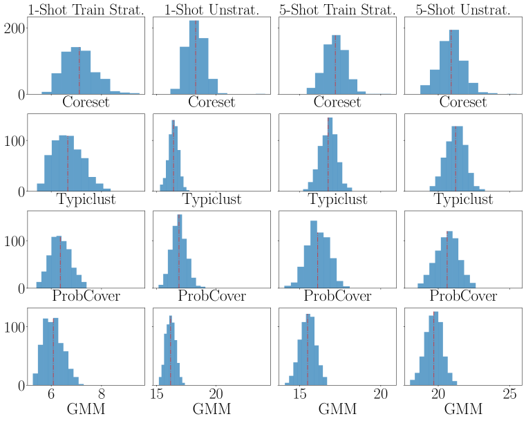
(a) Distributions of distances

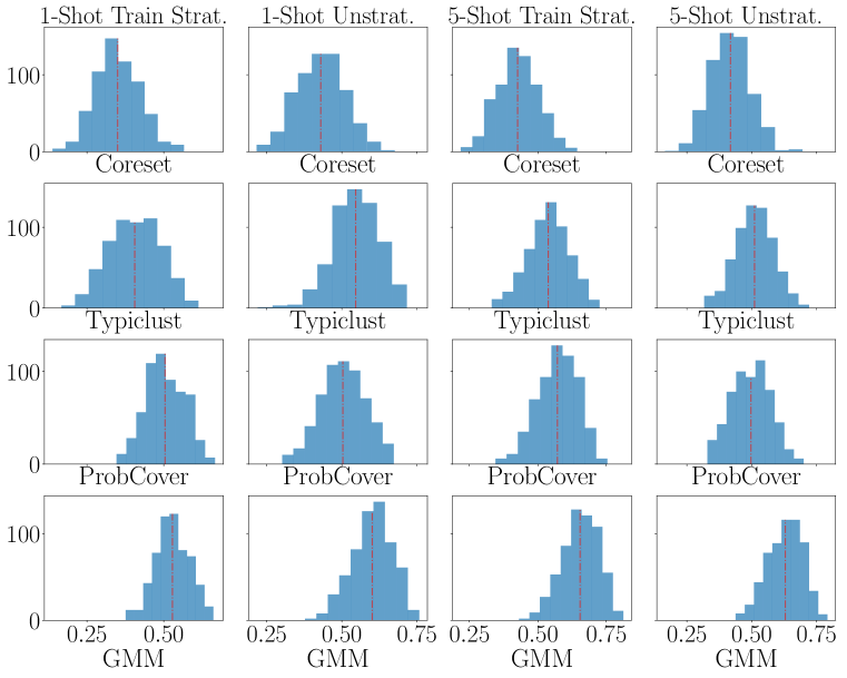
(b) Distributions of accuracies

Figure 6: Estimation of goodness of selected data points on MiniImageNet with ANIL using the distribution of (a) the distance between the unlabeled points and closest selected points, and (b) the equality between the true labels of unlabeled points and labels of the closest select points. Red dotted lines show mean values.

Data & Model	Clustering	1-Shot			5-Shot
		Fully strat.	Train strat.	Unstrat.	Fully strat.	Train strat.	Unstrat.
MiniImage. MAML	$k$-means	56.75 $\pm$ 0.20	33.29 $\pm$ 0.26	37.26 $\pm$ 0.18	65.76 $\pm$ 0.18	41.61 $\pm$ 0.24	59.17 $\pm$ 0.20
	Weighted Ent.	55.91 $\pm$ 0.34	22.69 $\pm$ 0.18	32.27 $\pm$ 0.32	63.87 $\pm$ 0.31	23.75 $\pm$ 0.25	46.80 $\pm$ 0.33
	GMM	58.82 $\pm$ 0.24	33.34 $\pm$ 0.24	37.68 $\pm$ 0.19	67.18 $\pm$ 0.18	54.35 $\pm$ 0.20	59.05 $\pm$ 0.20
FC100 ProtoNet	$k$-means	50.20 $\pm$ 0.17	29.69 $\pm$ 0.20	35.03 $\pm$ 0.23	54.07 $\pm$ 0.17	41.42 $\pm$ 0.23	41.34 $\pm$ 0.23
	Weighted Ent.	50.22 $\pm$ 0.18	31.80 $\pm$ 0.20	28.94 $\pm$ 0.19	50.38 $\pm$ 0.16	40.40 $\pm$ 0.25	39.95 $\pm$ 0.25
	GMM	50.22 $\pm$ 0.18	34.23 $\pm$ 0.23	35.03 $\pm$ 0.23	54.76 $\pm$ 0.17	46.30 $\pm$ 0.21	47.03 $\pm$ 0.20

Table 6: Comparison of GMM and $k$-Means selections on MiniImageNet and FC100 using MAML and ProtoNet.

Appendix E Comparison to $k$-Means based methods

Table 6 compares the proposed GMM method to $k$-means and weighted $k$-means (Nguyen & Smeulders, 2004; Donmez et al., 2007) on MiniImageNet and FC100 datasets with MAML and ProtoNet, respectively.

Nguyen & Smeulders (2004); Donmez et al. (2007) combines uncertainty and density-based sampling e.g. $k$-means for binary classification using logistic regression. For their original tasks, the selection criterion is equivalent to density weighted margin sampling. We extend it to $K$ way multi-class classification tasks where their acquisition criterion becomes weighted entropy.

For most cases, weighted entropy is constantly worse than the other two methods. It is expected since uncertainty-based criteria perform significantly worse than density-based criteria throughout all the experiments.

Also, the performance of GMM and $k$-means is similar in general but for some cases, GMM is significantly better than $k$-means. We conjecture it is because some features are more important than the others, and since GMM takes it into account using Mahalanobis distance (instead of Euclidean distance used in $k$-means), it selects data points that represents nearby data points better.

Appendix F Difficulty of Tuning the Radius Parameter for ProbCover

In Section 3.2 of Yehuda et al. (2022), the authors proposed to tune the radius $\delta$ based on the purity defined as,

$$\pi(\delta)=P(\{x:B_{\delta}(x)\text{ is pure}\})\,\,\,\text{ where }\,\,\,B_{\delta}(x)=\{x^{\prime}:\lVert x^{\prime}-x\rVert_{2}\leq\delta\}$$ (5)

Here, a ball $B_{\delta}(x)$ is “pure" if $f(x^{\prime})=y,\,\forall x^{\prime}\in B_{\delta}(x)$ where $y$ is the label of $x$. As the radius $\delta$ increases, the purity decreases monotonically. They choose the optimal radius $\delta^{*}$ as $\delta^{*}=\max\{\delta:\pi(\delta)\geq 0.95\}$. More specifically, they first run k-means with k being the number of classes. Then, the purity is measured using the k-means assignment as pseudo-labels.

In their setting (pool-based active learning for image classification), since it is hard to obtain meaningful features from a model trained only a few examples, they use the features from self-supervised learning methods such as SimCLR (Chen et al., 2020) It is, however, not the case for meta-learning. In meta-test time, the features from the meta learner are usually more meaningful than self-supervised learning features. Hence, we use the mete learner’s features to estimate the optimal radius for ProbCover. Following the original paper, we first run k-means and compute the purity in the same way. Since the features can differ by meta learning algorithms and the number of shots, we provide the plots for different algorithms as well as 1 and 5-Shots as shown in Figure 7 (we select the optimal radius $\delta$ based on these plots throughout the experiments). For Figure 7(a)-(f), we also provide the meta-test performance of stratified and unstratified versions of Random selection to demonstrate that the estimated optimal radius and best radius for meta-test accuracy do not align.

Another difficulty of estimating the optimal radius is that it is hard to set a search space for the radius. As shown in the x-axis of Figure 7, the reasonable search space varies significantly depending on the meta-learning algorithms and datasets we use. In Yehuda et al. (2022), this was less of a problem since they use SimCLR features, which are normalized: the range of the radius is in $[0,1]$. However, as shown in Appendix I, if we use SimCLR features in meta-test time to actively select context sets, the performance generally drops.

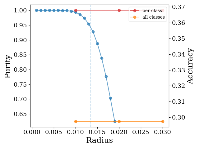
(a) Proto FC100 1-Shot

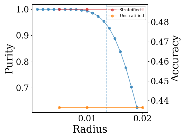
(b) Proto FC100 1-Shot

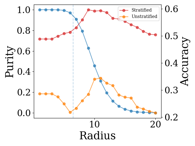
(c) MAML Mini. 1-Shot

(d) MAML Mini. 5-Shot

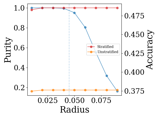
(e) ANIL Tiered. 1-Shot

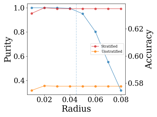
(f) ANIL Tiered. 5-Shot

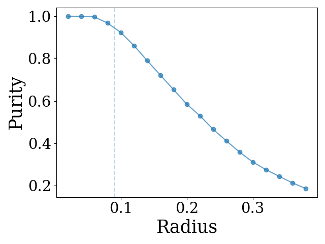
(g) Baseline++ CUB

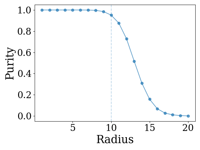
(h) SimpleShot Mini.

Figure 7: Estimation of the optimal radius for ProbCover in meta-learning

Appendix G Additional Experimental Results for Classification

In this section, we provide addtional experimental results for few-shot image classification. In Table 7, we compare the active learning strategies for ANIL (Raghu et al., 2020) on the TieredImageNet dataset. Similarly, Table 8 provides the results with MetaOptNet (Lee et al., 2019b) on FC100 dataset. Table 9, Table 10, and Table 11 are for SimpleShot (Wang et al., 2019), ProtoNet (Snell et al., 2017), and ANIL (Raghu et al., 2020) on MiniImageNet, respectively. Note that Entropy and Margin selections are not applicable for MetaOptNet-SVM. Regardless of meta-learning algorithm and dataset, GMM significantly outperforms the other active learning methods, and some of them are worse than the Random selection.

Appendix H Additional Experimental Details for Regression

Gao et al. (2022) propose the Distractor and ShapeNet1D datasets to compare meta learning algorithms for vision regression tasks. They evaluate meta learners for intra-category (IC) and cross-category (CC) inputs where CC corresponds to the cross-domain in few-shot image classification.

Distractor consists of $10$ object classes for a training set and $2$ novel classes for CC evaluation. Each class contains $1,000$ randomly sampled objects from ShapeNetCoreV2 (Chang et al., 2015). $20\%$ of training set is reserved for IC evaluation. In this dataset, each image consists of two objects: the object of interest and a distractor object, which are positioned randomly. The goal is to recognize and locate the object of interest within the image in the presence of a distractor.

ShapeNet1D (Gao et al., 2022) consists of $27$ object classes for a training set and $3$ object classes for CC evaluation. Each object class contains $50$ images, and $10$ images are used for IC evaluation. ShapeNet1D aims to predict the 1D pose, i.e., rotation angle, around the azimuth axis of an object.

To analyze these vision regression tasks, we compare various active learning strategies in the 2-shot setting. We use CNP for Distractor, NP for ShapeNet1D. More details about the models can be found in Appendix B.

$\operatorname{Pick}_{\theta}^{\mathit{eval}}$	1-Shot			5-Shot
	Fully strat.	Train strat.	Unstrat.	Fully strat.	Train strat.	Unstrat.
Random	$47.55\pm 0.18$	$38.19\pm 0.16$	$34.79\pm 0.15$	$63.84\pm 0.17$	$57.92\pm 0.23$	$57.56\pm 0.18$
Entropy	$43.89\pm 0.16$	$32.73\pm 0.16$	$26.33\pm 0.14$	$57.56\pm 0.18$	$40.23\pm 0.18$	$34.16\pm 0.17$
Margin	$47.35\pm 0.17$	$36.01\pm 0.14$	$30.79\pm 0.14$	$62.87\pm 0.17$	$54.89\pm 0.24$	$56.76\pm 0.17$
DPP	$49.28\pm 0.17$	$38.17\pm 0.15$	$36.52\pm 0.15$	$63.24\pm 0.19$	$57.28\pm 0.21$	$57.23\pm 0.18$
Coreset	$47.32\pm 0.18$	$36.97\pm 0.20$	$40.72\pm 0.14$	$56.93\pm 0.18$	$47.68\pm 0.22$	$52.89\pm 0.17$
Typiclust	$52.95\pm 0.18$	$37.21\pm 0.17$	$34.05\pm 0.14$	$63.13\pm 0.19$	$55.84\pm 0.22$	$56.76\pm 0.17$
ProbCover	$48.53\pm 0.53$	$37.61\pm 0.49$	$34.53\pm 0.43$	$63.48\pm 0.51$	57.77 $\pm$ 0.56	$57.12\pm 0.58$
GMM (Ours)	$60.29\pm 0.19$	$50.92\pm 0.22$	$42.17\pm 0.17$	$66.48\pm 0.18$	$60.12\pm 0.24$	$60.28\pm 0.17$

Table 7: 5-Way K-Shot classification on TieredImageNet with ANIL, with $\operatorname{Pick}_{\theta}^{\mathit{train}}$ random.

$\operatorname{Pick}_{\theta}^{\mathit{eval}}$	1-Shot			5-Shot
	Fully strat.	Train strat.	Unstrat.	Fully strat.	Train strat.	Unstrat.
Random	40.41 $\pm$ 0.74	31.96 $\pm$ 0.56	32.76 $\pm$ 0.63	53.11 $\pm$ 0.66	47.73 $\pm$ 0.70	47.48 $\pm$ 0.76
DPP	40.47 $\pm$ 0.80	30.33 $\pm$ 0.67	33.41 $\pm$ 0.66	51.44 $\pm$ 0.68	48.21 $\pm$ 0.67	47.45 $\pm$ 0.68
Coreset	39.20 $\pm$ 0.71	27.55 $\pm$ 0.66	30.16 $\pm$ 0.69	46.80 $\pm$ 0.67	24.08 $\pm$ 0.65	25.75 $\pm$ 0.72
Typiclust	45.20 $\pm$ 0.78	26.35 $\pm$ 0.47	27.00 $\pm$ 0.43	52.39 $\pm$ 0.66	23.97 $\pm$ 0.42	24.12 $\pm$ 0.39
ProbCover	41.93 $\pm$ 0.67	26.87 $\pm$ 0.62	27.43 $\pm$ 0.48	54.36 $\pm$ 0.76	37.00 $\pm$ 0.69	38.33 $\pm$ 0.76
GMM (Ours)	51.16 $\pm$ 0.67	40.89 $\pm$ 0.74	41.61 $\pm$ 0.87	60.48 $\pm$ 0.86	52.68 $\pm$ 0.70	51.79 $\pm$ 0.70

Table 8: 5-Way K-Shot classification on FC100 with MetaOptNet, with $\operatorname{Pick}_{\theta}^{\mathit{train}}$ random.

$\operatorname{Pick}_{\theta}^{\mathit{eval}}$	1-Shot		5-Shot
	Fully strat.	Train strat.	Fully strat.	Train strat.
Random	$45.15\pm 0.73$	$26.28\pm 0.61$	61.22 $\pm$ 0.72	51.89 $\pm$ 0.73
Entropy	$37.08\pm 0.75$	$21.62\pm 0.37$	$47.93\pm 0.74$	$32.74\pm 0.60$
Margin	$41.53\pm 0.73$	$24.28\pm 0.51$	62.15 $\pm$ 0.70	50.90 $\pm$ 0.75
DPP	$44.52\pm 0.75$	26.32 $\pm$ 0.58	$60.93\pm 0.72$	51.79 $\pm$ 0.75
Coreset	45.85 $\pm$ 0.73	27.04 $\pm$ 0.54	$56.48\pm 0.72$	$40.39\pm 0.68$
Typiclust	$44.53\pm 0.71$	$22.97\pm 0.42$	$34.21\pm 0.77$	$20.04\pm 0.06$
ProbCover	49.32 $\pm$ 0.71	$24.61\pm 0.52$	$55.60\pm 0.66$	$32.24\pm 0.67$
GMM (Ours)	52.77 $\pm$ 0.72	28.17 $\pm$ 0.64	62.64 $\pm$ 0.71	$50.40\pm 0.75$

Table 9: 5-Way K-Shot classification on MiniImageNet with SimpleShot, with $\operatorname{Pick}_{\theta}^{\mathit{train}}$ random.

$\operatorname{Pick}_{\theta}^{\mathit{eval}}$	1-Shot			5-Shot
	Fully strat.	Train strat.	Unstrat.	Fully strat.	Train strat.	Unstrat.
Random	47.70 $\pm$ 0.20	39.65 $\pm$ 0.28	38.72 $\pm$ 0.27	64.66 $\pm$ 0.18	57.36 $\pm$ 0.27	57.42 $\pm$ 0.25
Entropy	44.33 $\pm$ 0.20	36.35 $\pm$ 0.28	34.87 $\pm$ 0.27	61.23 $\pm$ 0.19	49.83 $\pm$ 0.31	48.46 $\pm$ 0.32
Margin	47.07 $\pm$ 0.20	37.69 $\pm$ 0.27	37.84 $\pm$ 0.28	63.79 $\pm$ 0.18	55.25 $\pm$ 0.29	56.15 $\pm$ 0.27
DPP	47.90 $\pm$ 0.20	39.17 $\pm$ 0.28	37.89 $\pm$ 0.26	64.36 $\pm$ 0.19	57.48 $\pm$ 0.26	57.37 $\pm$ 0.25
Coreset	47.86 $\pm$ 0.20	39.51 $\pm$ 0.26	37.79 $\pm$ 0.26	55.09 $\pm$ 0.20	50.14 $\pm$ 0.29	50.27 $\pm$ 0.28
Typiclust	59.51 $\pm$ 0.17	38.47 $\pm$ 0.27	37.57 $\pm$ 0.27	61.02 $\pm$ 0.19	51.82 $\pm$ 0.31	52.02 $\pm$ 0.30
ProbCover	48.51 $\pm$ 0.20	35.25 $\pm$ 0.26	34.50 $\pm$ 0.25	43.61 $\pm$ 0.19	38.63 $\pm$ 0.21	38.24 $\pm$ 0.20
GMM (Ours)	64.50 $\pm$ 0.16	47.88 $\pm$ 0.32	44.71 $\pm$ 0.29	67.03 $\pm$ 0.19	57.55 $\pm$ 0.29	56.44 $\pm$ 0.30

Table 10: 5-Way K-Shot classification on MiniImageNet with ProtoNet, with $\operatorname{Pick}_{\theta}^{\mathit{train}}$ random. The first, second, third best results for each setting are marked in this and all other results tables.

$\operatorname{Pick}_{\theta}^{\mathit{eval}}$	1-Shot			5-Shot
	Fully strat.	Train strat.	Unstrat.	Fully strat.	Train strat.	Unstrat.
Random	46.59 $\pm$ 0.19	36.70 $\pm$ 0.19	34.79 $\pm$ 0.18	61.35 $\pm$ 0.19	55.24 $\pm$ 0.20	56.65 $\pm$ 0.19
Entropy	44.63 $\pm$ 0.20	35.51 $\pm$ 0.18	27.35 $\pm$ 0.14	55.09 $\pm$ 0.19	39.71 $\pm$ 0.20	37.45 $\pm$ 0.19
Margin	46.58 $\pm$ 0.19	36.60 $\pm$ 0.19	32.46 $\pm$ 0.18	55.62 $\pm$ 0.19	40.40 $\pm$ 0.20	37.67 $\pm$ 0.19
DPP	47.33 $\pm$ 0.19	37.45 $\pm$ 0.17	37.76 $\pm$ 0.18	61.08 $\pm$ 0.19	56.18 $\pm$ 0.18	57.08 $\pm$ 0.18
Coreset	46.40 $\pm$ 0.21	38.37 $\pm$ 0.17	41.34 $\pm$ 0.17	53.74 $\pm$ 0.20	47.81 $\pm$ 0.20	51.62 $\pm$ 0.19
Typiclust	54.44 $\pm$ 0.18	36.78 $\pm$ 0.17	34.52 $\pm$ 0.19	60.87 $\pm$ 0.18	52.56 $\pm$ 0.20	55.11 $\pm$ 0.19
ProbCover	51.56 $\pm$ 0.18	27.49 $\pm$ 0.15	41.46 $\pm$ 0.17	61.68 $\pm$ 0.18	53.80 $\pm$ 0.20	42.70 $\pm$ 0.22
GMM (Ours)	58.50 $\pm$ 0.18	48.13 $\pm$ 0.20	40.26 $\pm$ 0.18	65.14 $\pm$ 0.17	59.01 $\pm$ 0.20	61.48 $\pm$ 0.19

Table 11: 5-Way K-Shot classification on MiniImageNet with ANIL, with $\operatorname{Pick}_{\theta}^{\mathit{train}}$ random.

Appendix I Comparison to Self-Supervised Features

ProbCover and Typiclust use self-supervised features to actively select new data points to annotate, since there are not enough labeled data to train a classifier to output meaningful features. Instead, they utilize the features from SimCLR (Chen et al., 2020). To validate if it is better to use the features from a meta learner than SimCLR in meta-learning, we compare SimCLR features to the features from either MAML or ProtoNet for Typiclust and ProbCover as shown in Table 12 and Table 13. Here, we use MiniImageNet and FC100 datasets for MAML and ProtoNet, respecitvely as with Table 2 and Table 1. For both Typiclust and ProbCover, although there are a couple of cases where SimCLR features are better, it is significantly worse than MAML and ProtoNet features in general. It intuitively makes sense because 1) meta learners are trained with large enough data points and 2) it is likely that the information in self-supervised features do not align with that in meta learners.

Dataset	Features	1-Shot			5-Shot
		Fully strat.	Train strat.	Unstrat.	Fully strat.	Train strat.	Unstrat.
Mini.	MAML	55.65 $\pm$ 0.18	27.45 $\pm$ 0.17	35.46 $\pm$ 0.18	64.16 $\pm$ 0.18	46.70 $\pm$ 0.21	57.83 $\pm$ 0.21
	SimCLR	44.84 $\pm$ 0.44	27.59 $\pm$ 0.35	34.80 $\pm$ 0.47	65.95 $\pm$ 0.43	36.03 $\pm$ 0.48	57.77 $\pm$ 0.47
FC100	ProtoNet	46.01 $\pm$ 0.16	30.96 $\pm$ 0.19	30.61 $\pm$ 0.21	47.54 $\pm$ 0.17	43.61 $\pm$ 0.18	44.03 $\pm$ 0.21
	SimCLR	36.07 $\pm$ 0.44	29.60 $\pm$ 0.46	30.13 $\pm$ 0.45	48.59 $\pm$ 0.49	43.29 $\pm$ 0.49	43.89 $\pm$ 0.59

Table 12: Comparison of MAML and SimCLR features for Typiclust in meta-test time.

Dataset	Features	1-Shot			5-Shot
		Fully strat.	Train strat.	Unstrat.	Fully strat.	Train strat.	Unstrat.
Mini.	MAML	52.81 $\pm$ 1.16	21.91 $\pm$ 0.24	36.21 $\pm$ 0.18	64.70 $\pm$ 0.91	42.07 $\pm$ 0.49	23.40 $\pm$ 0.36
	SimCLR	47.57 $\pm$ 0.42	25.35 $\pm$ 0.38	32.19 $\pm$ 0.43	64.33 $\pm$ 0.39	36.64 $\pm$ 0.58	26.16 $\pm$ 0.43
FC100	ProtoNet	48.66 $\pm$ 0.16	32.86 $\pm$ 0.22	33.58 $\pm$ 0.19	51.11 $\pm$ 0.17	44.20 $\pm$ 0.24	44.40 $\pm$ 0.24
	SimCLR	31.40 $\pm$ 0.42	29.53 $\pm$ 0.42	28.39 $\pm$ 0.43	47.11 $\pm$ 0.39	39.33 $\pm$ 0.54	45.40 $\pm$ 0.52

Table 13: Comparison of MAML and SimCLR features for ProbCover in meta-test time.

Appendix J Training-Time Active Learning

As mentioned in Section 5, we observe that active learning methods do not significantly change the generalization performance of meta learners when applied in meta-train time, which aligns with Ni et al. (2021) and Setlur et al. (2020). To empirically demonstrate the statement, we apply several active learning methods without stratification in the meta-train time for ProtoNet on MiniImageNet. Again, we report the mean and $95\%$ confidence interval from $600$ meta-test tasks. Figure 8 shows among Random, DPP and GMM selections, one is not significantly better than another although the Entropy selection is significantly worse than them.

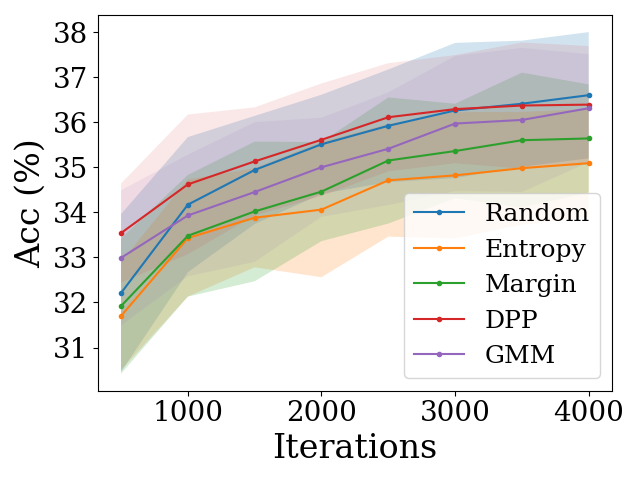
Figure 8: Comparison of $\operatorname{Pick}_{\theta}^{\mathit{train}}$.

Appendix K Sequential Active-Meta Learning

Figure 9 compare active learning methods for sequential setting where we select $5$ context samples at a time until the budget reaches $25$ samples. Every time we select new context samples we may utilize them to maximize new label information. For MAML, we update all the model parameters through adaptation steps. It is, however, not applicable to the other meta-learning methods we use in this work including ProtoNet, since none of the other methods including optimization-based methods such as ANIL, do not update the parameters up to the penultimate layer.

As expected, the test performance of ProtoNet does not change much regardless of active learning methods. But, the test performance of MAML gradually increases as we add more context samples. In sequential active-meta learning, GMM still significantly outperforms other active learning methods.

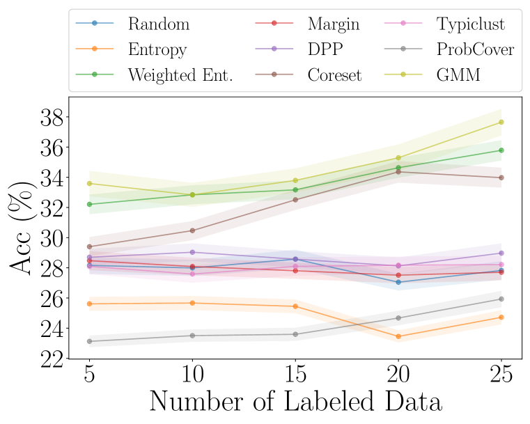
(a) MAML – Train strat.

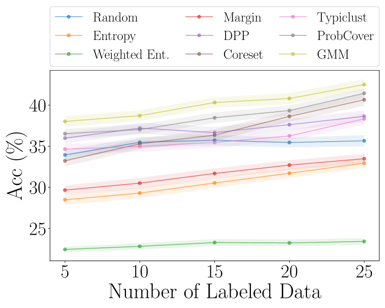
(b) MAML – Unstrat.

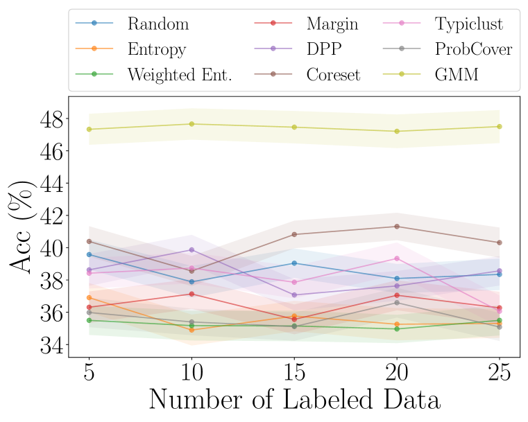
(c) Proto – Train strat.

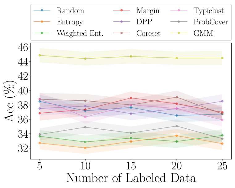
(d) Proto – Unstrat.

Figure 9: Test performance of MAML and ProtoNet on MiniImageNet with sequentially actively selected context sets. $5$ context samples are selected at each iteration until it reaches $25$.

References

- Agarwal et al. (2021) Mayank Agarwal, Mikhail Yurochkin, and Yuekai Sun. On sensitivity of meta-learning to support data. NeurIPS, 2021.
- Aghaee et al. (2016) Amin Aghaee, Mehrdad Ghadiri, and Mahdieh Soleymani Baghshah. Active distance-based clustering using k-medoids. In PAKDD, 2016.
- Antoniou et al. (2019) Antreas Antoniou, Harrison Edwards, and Amos Storkey. How to train your MAML. In ICLR, 2019.
- Arnold et al. (2020) Sébastien M R Arnold, Praateek Mahajan, Debajyoti Datta, Ian Bunner, and Konstantinos Saitas Zarkias. learn2learn: A library for Meta-Learning research. 2020.
- Ash et al. (2020) Jordan T Ash, Chicheng Zhang, Akshay Krishnamurthy, John Langford, and Alekh Agarwal. Deep batch active learning by diverse, uncertain gradient lower bounds. ICLR, 2020.
- Bertinetto et al. (2019) Luca Bertinetto, João F. Henriques, Philip H. S. Torr, and Andrea Vedaldi. Meta-learning with differentiable closed-form solvers. In ICLR, 2019.
- Bıyık et al. (2019) Erdem Bıyık, Kenneth Wang, Nima Anari, and Dorsa Sadigh. Batch active learning using determinantal point processes. NeurIPS, 2019.
- Boney & Ilin (2017) Rinu Boney and Alexander Ilin. Semi-supervised and active few-shot learning with prototypical networks. 2017.
- Chang et al. (2015) Angel X Chang, Thomas Funkhouser, Leonidas Guibas, Pat Hanrahan, Qixing Huang, Zimo Li, Silvio Savarese, Manolis Savva, Shuran Song, Hao Su, Jianxiong Xiao, Li Yi, and Fisher Yu. ShapeNet: An information-rich 3D model repository. 2015.
- Chen et al. (2020) Ting Chen, Simon Kornblith, Mohammad Norouzi, and Geoffrey Hinton. A simple framework for contrastive learning of visual representations. In ICML, 2020.
- Chen et al. (2019) Wei-Yu Chen, Yen-Cheng Liu, Zsolt Kira, Yu-Chiang Frank Wang, and Jia-Bin Huang. A closer look at few-shot classification. 2019.
- Crammer & Singer (2001) Koby Crammer and Yoram Singer. On the algorithmic implementation of multiclass kernel-based vector machines. JMLR, 2001.
- Deng et al. (2009) Jia Deng, Wei Dong, Richard Socher, Li-Jia Li, Kai Li, and Li Fei-Fei. ImageNet: A large-scale hierarchical image database. In CVPR, 2009.
- Donmez et al. (2007) Pinar Donmez, Jaime G Carbonell, and Paul N Bennett. Dual strategy active learning. In ECML, 2007.
- Dubois et al. (2020) Yann Dubois, Jonathan Gordon, and Andrew YK Foong. Neural process family. http://yanndubs.github.io/Neural-Process-Family/, 2020.
- Fang et al. (2017) Meng Fang, Yuan Li, and Trevor Cohn. Learning how to active learn: A deep reinforcement learning approach. In EMNLP, 2017.
- Finn et al. (2017) Chelsea Finn, Pieter Abbeel, and Sergey Levine. Model-agnostic meta-learning for fast adaptation of deep networks. In ICML, 2017.
- Finn et al. (2018) Chelsea Finn, Kelvin Xu, and Sergey Levine. Probabilistic model-agnostic meta-learning. In NeurIPS, 2018.
- Freytag et al. (2014) Alexander Freytag, Erik Rodner, and Joachim Denzler. Selecting influential examples: Active learning with expected model output changes. In ECCV, 2014.
- Gao et al. (2022) Ning Gao, Hanna Ziesche, Ngo Anh Vien, Michael Volpp, and Gerhard Neumann. What matters for meta-learning vision regression tasks? In CVPR, 2022.
- Garnelo et al. (2018a) Marta Garnelo, Dan Rosenbaum, Christopher Maddison, Tiago Ramalho, David Saxton, Murray Shanahan, Yee Whye Teh, Danilo Rezende, and SM Ali Eslami. Conditional neural processes. In ICML, 2018a.
- Garnelo et al. (2018b) Marta Garnelo, Jonathan Schwarz, Dan Rosenbaum, Fabio Viola, Danilo J Rezende, SM Eslami, and Yee Whye Teh. Neural processes. In ICML Workshop on Theoretical Foundations and Applications of Deep Generative Models, 2018b.
- Garnett et al. (2012) Roman Garnett, Yamuna Krishnamurthy, Xuehan Xiong, Jeff Schneider, and Richard Mann. Bayesian optimal active search and surveying. In ICML, 2012.
- Gautier et al. (2019) Guillaume Gautier, Guillermo Polito, Rémi Bardenet, and Michal Valko. DPPy: DPP sampling with Python. JMLR-MLOSS, 2019. URL https://github.com/guilgautier/DPPy/.
- Goldblum et al. (2020) Micah Goldblum, Steven Reich, Liam Fowl, Renkun Ni, Valeriia Cherepanova, and Tom Goldstein. Unraveling meta-learning: Understanding feature representations for few-shot tasks. In ICML, 2020.
- Gordon et al. (2020) Jonathan Gordon, Wessel P Bruinsma, Andrew YK Foong, James Requeima, Yann Dubois, and Richard E Turner. Convolutional conditional neural processes. In ICLR, 2020.
- Guo & Greiner (2007) Yuhong Guo and Russell Greiner. Optimistic active-learning using mutual information. In IJCAI, 2007.
- Hacohen et al. (2022) Guy Hacohen, Avihu Dekel, and Daphna Weinshall. Active learning on a budget: Opposite strategies suit high and low budgets. ICML, 2022.
- He et al. (2016) Kaiming He, Xiangyu Zhang, Shaoqing Ren, and Jian Sun. Deep residual learning for image recognition. In CVPR, 2016.
- Hilliard et al. (2018) Nathan Hilliard, Lawrence Phillips, Scott Howland, Artëm Yankov, Courtney D Corley, and Nathan O Hodas. Few-shot learning with metric-agnostic conditional embeddings. 2018.
- Hospedales et al. (2022) Timothy Hospedales, Antreas Antoniou, Paul Micaelli, and Amos Storkey. Meta-learning in neural networks: A survey. PAMI, 44(9):5149–5169, 2022.
- Kaddour et al. (2020) Jean Kaddour, Steindór Sæmundsson, and Marc Peter Deisenroth. Probabilistic active meta-learning. In NeurIPS, 2020.
- Käding et al. (2016) Christoph Käding, Erik Rodner, Alexander Freytag, and Joachim Denzler. Active and continuous exploration with deep neural networks and expected model output changes. In NeurIPS Workshop on Continual Learning and Deep Networks, 2016.
- Käding et al. (2018) Christoph Käding, Erik Rodner, Alexander Freytag, Oliver Mothes, Björn Barz, Joachim Denzler, and Carl Zeiss AG. Active learning for regression tasks with expected model output changes. In BMVC, 2018.
- Kim et al. (2019) Hyunjik Kim, Andriy Mnih, Jonathan Schwarz, Marta Garnelo, Ali Eslami, Dan Rosenbaum, Oriol Vinyals, and Yee Whye Teh. Attentive neural processes. In ICLR, 2019.
- Konyushkova et al. (2017) Ksenia Konyushkova, Raphael Sznitman, and Pascal Fua. Learning active learning from data. In NeurIPS, 2017.
- Krizhevsky (2009) Alex Krizhevsky. Learning multiple layers of features from tiny images. 2009.
- Kumar et al. (2022) Ramnath Kumar, Tristan Deleu, and Yoshua Bengio. The effect of diversity in meta-learning. 2022.
- Lang et al. (2021) Adrian Lang, Christoph Mayer, and Radu Timofte. Best practices in pool-based active learning for image classification. 2021.
- Lee et al. (2019a) Jaehoon Lee, Lechao Xiao, Samuel Schoenholz, Yasaman Bahri, Roman Novak, Jascha Sohl-Dickstein, and Jeffrey Pennington. Wide neural networks of any depth evolve as linear models under gradient descent. In NeurIPS, 2019a.
- Lee et al. (2019b) Kwonjoon Lee, Subhransu Maji, Avinash Ravichandran, and Stefano Soatto. Meta-learning with differentiable convex optimization. In CVPR, 2019b.
- Mohamadi et al. (2022) Mohamad Amin Mohamadi, Wonho Bae, and Danica J. Sutherland. Making look-ahead active learning strategies feasible with neural tangent kernels. In NeurIPS, 2022.
- Müller et al. (2022) Thomas Müller, Guillermo Pérez-Torró, Angelo Basile, and Marc Franco-Salvador. Active few-shot learning with fasl. In NLDB, 2022.
- Munjal et al. (2022) Prateek Munjal, Nasir Hayat, Munawar Hayat, Jamshid Sourati, and Shadab Khan. Towards robust and reproducible active learning using neural networks. In CVPR, 2022.
- Nguyen & Smeulders (2004) Hieu T Nguyen and Arnold Smeulders. Active learning using pre-clustering. In ICML, 2004.
- Ni et al. (2021) Renkun Ni, Micah Goldblum, Amr Sharaf, Kezhi Kong, and Tom Goldstein. Data augmentation for meta-learning. In ICML, 2021.
- Nikoloska & Simeone (2022) Ivana Nikoloska and Osvaldo Simeone. Bamld: Bayesian active meta-learning by disagreement. SPAWC, 2022.
- Oh et al. (2022) Jaehoon Oh, Sungnyun Kim, Namgyu Ho, Jin-Hwa Kim, Hwanjun Song, and Se-Young Yun. Understanding cross-domain few-shot learning based on domain similarity and few-shot difficulty. In NeurIPS, 2022.
- Oreshkin et al. (2018) Boris Oreshkin, Pau Rodríguez López, and Alexandre Lacoste. Tadam: Task dependent adaptive metric for improved few-shot learning. In NeurIPS, 2018.
- Pezeshkpour et al. (2020) Pouya Pezeshkpour, Zhengli Zhao, and Sameer Singh. On the utility of active instance selection for few-shot learning. In HAMLETS workshop at NeurIPS, 2020.
- Raghu et al. (2020) Aniruddh Raghu, Maithra Raghu, Samy Bengio, and Oriol Vinyals. Rapid learning or feature reuse? towards understanding the effectiveness of maml. In ICLR, 2020.
- Ravi & Larochelle (2017) Sachin Ravi and Hugo Larochelle. Optimization as a model for few-shot learning. In ICLR, 2017.
- Ren et al. (2018) Mengye Ren, Eleni Triantafillou, Sachin Ravi, Jake Snell, Kevin Swersky, Joshua B Tenenbaum, Hugo Larochelle, and Richard S Zemel. Meta-learning for semi-supervised few-shot classification. In ICLR, 2018.
- Ren et al. (2021) Pengzhen Ren, Yun Xiao, Xiaojun Chang, Po-Yao Huang, Zhihui Li, Brij B. Gupta, Xiaojiang Chen, and Xin Wang. A survey of deep active learning. ACM Comput. Surv., 54(9), 10 2021.
- Roy & McCallum (2001) Nicholas Roy and Andrew McCallum. Toward optimal active learning through monte carlo estimation of error reduction. In ICML, 2001.
- Scheffer et al. (2001) Tobias Scheffer, Christian Decomain, and Stefan Wrobel. Active hidden markov models for information extraction. In ISIDA, 2001.
- Sener & Savarese (2018) Ozan Sener and Silvio Savarese. Active learning for convolutional neural networks: A core-set approach. ICLR, 2018.
- Setlur et al. (2020) Amrith Setlur, Oscar Li, and Virginia Smith. Is support set diversity necessary for meta-learning? 2020.
- Settles (2009) Burr Settles. Active learning literature survey. 2009.
- Settles et al. (2007) Burr Settles, Mark Craven, and Soumya Ray. Multiple-instance active learning. 2007.
- Snell et al. (2017) Jake Snell, Kevin Swersky, and Richard S Zemel. Prototypical networks for few-shot learning. In NeurIPS, 2017.
- Soudry et al. (2018) Daniel Soudry, Elad Hoffer, Mor Shpigel Nacson, Suriya Gunasekar, and Nathan Srebro. The implicit bias of gradient descent on separable data. JMLR, 2018.
- van der Maaten & Hinton (2008) Laurens van der Maaten and Geoffrey Hinton. Visualizing data using t-sne. JMLR, 2008.
- Vinyals et al. (2016) Oriol Vinyals, Charles Blundell, Timothy Lillicrap, Daan Wierstra, et al. Matching networks for one shot learning. In NeurIPS, 2016.
- Voevodski et al. (2012) Konstantin Voevodski, Maria-Florina Balcan, Heiko Röglin, Shang-Hua Teng, and Yu Xia. Active clustering of biological sequences. JMLR, 2012.
- Wah et al. (2011) Catherine Wah, Steve Branson, Peter Welinder, Pietro Perona, and Serge Belongie. The Caltech-UCSD Birds-200-2011 dataset. California Institute of Technology technical report CNS-TR-2011-001, 2011.
- Wang & Shang (2014) Dan Wang and Yi Shang. A new active labeling method for deep learning. In IJCNN, 2014.
- Wang et al. (2019) Yan Wang, Wei-Lun Chao, Kilian Q. Weinberger, and Laurens van der Maaten. Simpleshot: Revisiting nearest-neighbor classification for few-shot learning. 2019.
- Yehuda et al. (2022) Ofer Yehuda, Avihu Dekel, Guy Hacohen, and Daphna Weinshall. Active learning through a covering lens. NeurIPS, 2022.
- Zhang et al. (2021) Xueting Zhang, Debin Meng, Henry Gouk, and Timothy M Hospedales. Shallow bayesian meta learning for real-world few-shot recognition. In ICCV, 2021.
- Zhou et al. (2017) Bolei Zhou, Agata Lapedriza, Aditya Khosla, Aude Oliva, and Antonio Torralba. Places: A 10 million image database for scene recognition. PAMI, 2017.
- Zhu et al. (2003) Xiaojin Zhu, John Lafferty, and Zoubin Ghahramani. Combining active learning and semi-supervised learning using gaussian fields and harmonic functions. In ICML Workshops, 2003.