Neural-based Compression Scheme for Solar Image Data

Abstract

Studying the solar system and especially the Sun relies on the data gathered daily from space missions. These missions are data-intensive and compressing this data to make them efficiently transferable to the ground station is a twofold decision to make. Stronger compression methods, by distorting the data, can increase data throughput at the cost of accuracy which could affect scientific analysis of the data. On the other hand, preserving subtle details in the compressed data requires a high amount of data to be transferred, reducing the desired gains from compression. In this work, we propose a neural network-based lossy compression method to be used in NASA’s data-intensive imagery missions. We chose NASA’s Solar Dynamics Observatory (SDO) mission which transmits 1.4 terabytes of data each day as a proof of concept for the proposed algorithm. In this work, we propose an adversarially trained neural network, equipped with local and non-local attention modules to capture both the local and global structure of the image resulting in a better trade-off in rate-distortion (RD) compared to conventional hand-engineered codecs. The RD variational autoencoder used in this work is jointly trained with a channel-dependent entropy model as a shared prior between the analysis and synthesis transforms to make the entropy coding of the latent code more effective. We also studied how optimizing perceptual losses could help our neural compressor to preserve high-frequency details of the data in the reconstructed compressed image. Our neural image compression algorithm outperforms currently-in-use and state-of-the-art codecs such as JPEG and JPEG-2000 in terms of the RD performance when compressing extreme-ultraviolet (EUV) data. As a proof of concept for use of this algorithm in SDO data analysis, we have performed coronal hole (CH) detection using our compressed images, and generated consistent segmentations, even at a compression rate of $\sim 0.1$ bits per pixel (compared to 8 bits per pixel on the original data) using EUV data from SDO.

1 Introduction

Learning based image compression outperform (Yang et al., 2022) almost all traditional codecs including JPEG (Wallace, 1991) and JPEG-2000 (Taubman & Marcellin, 2002). With a basis in convolutional neural networks (CNNs), the performance of said learned compression methods has been improved through various investigations: enhanced entropy model (Minnen et al., 2018; Minnen & Singh, 2020; Qian et al., 2022), learned representation augmentation via attention (Cheng et al., 2020; Zhu et al., 2022) and incorporating adversarial training for improved perceptual quality of reconstruction (Agustsson et al., 2019; Blau & Michaeli, 2019; Mentzer et al., 2020a).

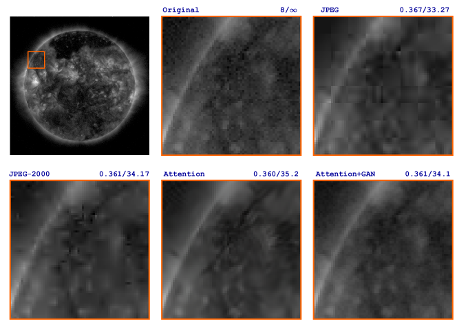
Figure 1: Visual comparison of proposed compression schemes (Attention only and GAN+Attention) to other standard codecs. Reported performance is in terms of bit-rate/distortion [bpp$\downarrow$/PSNR$\uparrow$]. GAN outputs are visually closer to the original input despite their inferior performance in terms of PSNR. Best viewed on screen.

In this work, we demonstrate the potential of neural network compression codecs to serve as the go-to approach for future space missions for on-board data compression. We baseline our novel algorithm on the solar image data collected by the Atmospheric Imaging Assembly (AIA) instrument on-board the Solar Dynamics Observatory (SDO) spacecraft and compare the performance with traditional methods. Finally, we show that a CH segmentation (Boucheron et al., 2016) is minimally affected even at extremely low bit-rate compression provided by our proposed neural compression method. Extremely compressed images using our network preserves the required details for the task of CH segmentation on images downloaded from the SDO mission.

Contributions of This Work. Preliminary results of our proposed algorithm is published in (Zafari et al., 2022), introducing the application of neural image compression on downloaded solar imagery data. The primary contribution of the current work is to critically evaluate the performance of our algorithm on downstream science and/or operational tasks (e.g. CH segmentation). Additionally, we provide a detailed description of the joint forward and backward adapted entropy model used to improve the rate-distortion performance of the proposed algorithm which was not available in (Zafari et al., 2022).

The paper is structured as follows: Section 2 provides a review of neural compression autoencoders and their potential application for a solar mission with a discussion of the downstream scientific task of segmentation on the SDO data. Section 3 is devoted to our proposed method. Experimental results and ablation studies are described in Section 4. Section 5 concludes our discussions.

2 Related Work

2.1 Neural Image Compression

Transform coding-based image compression algorithms share four main steps to compress an image (Goyal, 2001). First, a transform is applied to the image to transfer the pixels from their spatial domain to a transform domain that reduces correlation between pixels and thereby results in many small coefficients (i.e., information packing). Second, the transformed image is quantized to discard less significant information from the data in the transform domain. Third, entropy coding is utilized to losslessly encode the quantized samples into a stream of ones and zeros. This bitstream is the compressed image. The fourth and final step occurs at the receiving end (or at the reconstructing step), which is responsible for decoding the quantized values to the original space of the input image. The first and most widely used architecture to mimic this scenario in deep neural networks is the convolutional autoencoder which has shown its superiority in terms of rate-distortion performance in the literature (Ballé et al., 2017). Both the encoding and decoding parts of the traditional transform codec can be imitated by an autoencoder (Ballé et al., 2021).

In an end-to-end optimization of an autoencoder, problems arise when we want to quantize the bottleneck to remove redundancies in order to reach high compression ratios. ANNs are optimized using gradient descent algorithms which update the parameters of the network by back-propagating the gradients of the loss function. Gradients of the quantization process are not useful for optimizing the loss function as its value is either zero or infinity. As a result, we need to approximate hard discrete quantization with an operation yielding informative gradients for updating the parameters of the network. The most widely used approach is proposed by (Ballé et al., 2016a), inherited from (Gray & Neuhoff, 1998), in which they showed that adding independent and identically distributed unit uniform noise can be interpreted equivalently as doing scalar quantization on the bottleneck. This method is thoroughly discussed in Section 3.1.3. By applying this noise to the bottleneck, we can optimize the differential entropy of the continuous approximation as a variational upper bound (Theis et al., 2016) to reduce the entropy of the bottleneck. Low entropy messages are compressed more efficiently into bitstreams (Cover, 1999).

Optimal compression in theory can be achieved by vector quantization (Gersho & Gray, 2012). In vector quantization each data point is represented by a prototype and a collection of prototypes, called a codebook, is shared between sender and receiver. The application of vector quantization in ANN-based compression has been investigated by (Agustsson et al., 2017), with the cost of a complicated training procedure. To make the training more accessible, neural compression algorithms follow the classical approach to avoid the complexity of vector quantization. In classical image compression schemes, e.g., JPEG (Wallace, 1991), to get the best out of the quantization process, the first step is to apply an invertible linear transform and translate the image into decorrelated coefficients using a linear transform, e.g., Discrete Cosine Transform (DCT) in JPEG (Wallace, 1991). By doing so, scalar quantization can reach a reasonable performance close to vector quantization (Goyal, 2001). On the other hand, it has been shown (Ballé et al., 2017; 2021) that a joint-optimized learned nonlinear transform, i.e., neural network, followed by scalar quantization is sufficient to approximate a parametric form of vector quantization.

As will be shown in Section 3, replacing the actual quantization of the latent code/bottleneck of the autoencoder with a uniform noise approximation in the bottleneck of a vanilla autoencoder during training of the network (Ballé et al., 2018) will transform it to a Variational Autoencoder (VAE) (Kingma & Ba, 2015b).

The difference between the rate-distortion VAE and its vanilla version is the chosen prior for the latent variables. In autoencoder-based image compression, the Gaussian prior of the VAE is replaced with a unit uniform distribution centered on integer numbers to imitate the scalar quantization process.

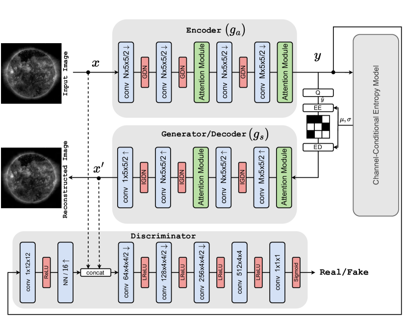
Figure 2: Network architecture. The input image traverses through a series of convolutional layers yielding 16 times smaller (spatially) feature maps than the original input dimensions. To reconstruct the image, the decoder follows the same dimensions of the encoder network in a reverse order using transpose convolution layers. A conditional discriminator encourages the generator (decoder) toward better perceptual quality. The number of channels in the encoder and decoder are set as $N=192$ and $M=320$, respectively. Q performs scalar quantization. EE and ED indicate the entropy encoder and decoder, respectively. The checkerboard box represents the bitstream of the compressed image including only zeros and ones. $\mu$ and $\sigma$ are predicted parameters of the latent code probability distribution, defined by the entropy estimation model as shown in Fig. 3. LReLU denotes Leaky Rectified Linear Unit activation function. GDN and IGDN correspond to Generalized Divisive Normalization nonlinearity and its inverse, discussed in Section 4.2.

2.2 Generative Adversarial Training

Generative Adversarial Networks (GANs) (Goodfellow et al., 2014) have emerged as a transformative technology in the fields of computer vision and aerospace systems, offering a wide array of innovative applications. In the realm of computer vision, GANs have played a pivotal role in image generation (Brock et al., 2019; Esser et al., 2021), enhancement (Poirier-Ginter & Lalonde, 2023), and manipulation (Ling et al., 2021). Researchers have leveraged GANs to generate high-resolution images from low-resolution inputs (Ledig et al., 2017), thereby enhancing the quality of visual data, a crucial advancement for various computer vision applications. GANs have also demonstrated their ability to generate realistic synthetic images (Brock et al., 2019; Esser et al., 2021), which find application in data augmentation for training deep neural network models, particularly in scenarios where labeled datasets are limited. Additionally, GANs have been instrumental in style transfer (Karras et al., 2019), enabling the creation of unique visual content by merging the style of one image with the content of another (Karras et al., 2020). GANs are also used in domain translation tasks to make realistic photos out of sketches or colorizing grayscale images (Isola et al., 2017; Zhu et al., 2017).

The utilization of GANs has been particularly noteworthy in the aerospace field of study. GANs have been employed to enhance satellite imagery for Earth observation and environmental monitoring (Jozdani et al., 2022). They facilitate the removal of sensor noise (Toner & Fletcher, 2022), the enhancement of image resolution, and the synthesis of missing data (Hu et al., 2022), or improving the overall quality of satellite-based remote sensing (Liu et al., 2022). GANs has shown great potential in synthesizing RF micro-Doppler signatures to tackle the challenge of limited sample availability and facilitate the training of more complex deep neural networks (DNNs) to improve RF signal classification performance (Rahman et al., 2022). Training neural networks in a GAN framework also improved unsupervised domain adaptation in satellite pose estimation (Wang et al., 2023). These advancements have the potential to significantly impact industries, from enhancing image analysis to improving the safety and efficiency of aerospace operations.

2.3 Attention Mechanism in Neural Networks

When it comes to computer vision, deep convolutional neural networks (CNNs) are the de facto standard despite their poor performance in capturing long-range dependencies (Li et al., 2021; Zhou et al., 2021). The performance degradation of CNNs is attributed to their local receptive field, which is mainly because of the limited kernel size (Ramachandran et al., 2019) of the filters.

Efforts have been made to help CNNs capture a more robust representation of the input image. One naïve solution is to make the network deeper, but other problems will arise in training such networks which have led to the introduction of deep residual networks (ResNet) (He et al., 2016). Although increasing the parameters of a network will generally lead to a richer representation and better performance, it will make training such networks harder since overfitting can easily happen in these over-parametrized neural networks. Attention mechanisms have been proposed to address the problem of the local receptive field by keeping the depth of the network unchanged. In (Wang et al., 2017) a single module was proposed to be included in between sequential convolutional layers, consisting of two branches, the trunk to process local features and the mask to decide which of the local features in the trunk are more important to be passed to the next convolutional layer, as in Fig. 4(a).

In contrast to local attention, the authors in (Wang et al., 2018) first discussed how non-local attention can be viewed as a special case of a non-local algorithm which was traditionally used as a method to denoise images (Buades et al., 2005). The idea was to find similar pixels/patches in the image/feature map and replace them with a weighted sum over all the others, with higher weights for more similar ones. It can be inferred from (Wang et al., 2018) that Vision Transformers (ViT) (Dosovitskiy et al., 2021) are all special cases of the non-local attention mechanism.

The non-local attention block (see Fig. 4(b)) helps the mask branch to efficiently learn the most informative parts of features (in the trunk) for the task at hand (Zhang et al., 2019). The authors in (Zhang et al., 2019) also added a skip connection to help the output feature maps be richer, by letting the module have access to both attended and raw features. This skip connection prevents vanishing gradients as well.

Another recently proposed mechanism to incorporate attention in CNNs has been introduced in (Woo et al., 2018). It is an enhanced version of the Squeeze-and-Excitation network (Hu et al., 2018), to apply attention on both spatial and channel feature maps separately. This way of applying attention is simpler and computationally more efficient than previous computation-heavy attention mechanisms based on pre-trained networks or complex calculations (Xiao et al., 2015).

3 Methods

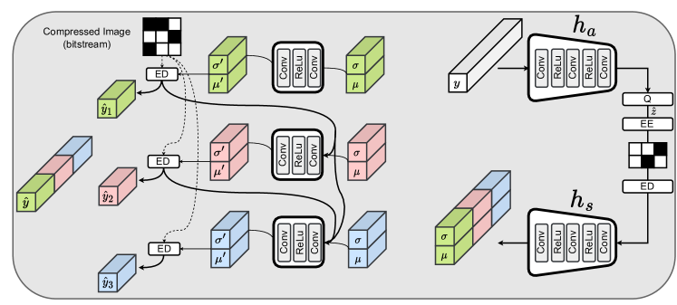
Figure 3: Joint forward and backward adaptation entropy model with the channel conditioning assumption in the probability distribution of the latents. Conv represents a convolutional layer with a kernel size of $3\times 3$ with stride and padding of size $1$. Due to limited space, this figure shows channel-wise conditioning on only three slices (red, green, and blue), while in the implementation the latent code is divided into 10 slices. After decoding, the first slice ($\bm{\hat{y}}_{1}$) is used to decode the second one ($\bm{\hat{y}}_{2}$), and both of them are used for decoding the third slice ($\bm{\hat{y}}_{3}$). ReLu stands for a rectified linear unit. Q, EE, and ED denote quantization, and entropy encoder/decoder, respectively. Checkerboard boxes represent bitstream codes. The estimated probability distribution that is parametrized by $\mu$ an $\sigma$ is shared as the prior over the latent code both on the encoder and decoder side at the time of entropy coding.

3.1 Generative Image Compression

Autoencoder-based learned image compression networks, like the one we have proposed in Fig. 2, generally consist of two major parts. The first part includes the encoder/decoder network and the second part is the bottleneck entropy estimation network. The former is discussed in this section and Section 3.1.2 is devoted to describing the functionality of the latter. As illustrated in Figs. 2 and 3, the network input ($\bm{x}$) and output ($\bm{x^{\prime}}$) relations can be summarized as follows:

$$\bm{x^{\prime}}=g_{s}(ED(EE(\bm{\hat{y}}));\bm{\theta_{g}}),$$ (1)

$$\bm{\hat{y}}=\lfloor g_{a}(\bm{x};\bm{\phi_{g}})\rceil,$$

$$\bm{\hat{z}}=\lfloor h_{a}(\bm{y};\bm{\phi_{h}})\rceil,$$

in which $\lfloor\cdot\rceil$ denotes the quantization of a real value to the nearest integer number, $\bm{\hat{y}}$ is the quantized latent variable, and $\bm{\hat{z}}$ is its quantized hyper-prior which is discussed in Section 3.1.2. $ED$ and $EE$ denote the entropy decoder and entropy encoder, respectively. The encoder and decoder nonlinear transforms are represented by $g_{a}$ and $g_{s}$ with their learned parameters, $\bm{\phi_{g}}$ and $\bm{\theta_{g}}$, respectively. The subscripts $a$ and $s$ refer to analysis and synthesis as they are common designations for the compression and decompression processes in the area of transform coding-based compression. $h_{a}$ is the analysis transform to get the hyper-priors of the entropy estimation model, defined by its parameters $\bm{\phi_{h}}$. Throughout the following section, we use the terms quantized bottleneck and quantized latent code interchangeably.

3.1.1 Learning Objective

Any learned image compression network tries to find an optimal tradeoff in the rate-distortion plane by trading off distortion for the expected bitrate (or vice versa), governed by a Lagrangian coefficient $\lambda$. The rate-distortion trade-off can be described as:

$$R+\lambda D_{r},$$ (2)

where $R$ and $D_{r}$ correspond to the estimated entropy of the latent code and reconstruction distortion, respectively. The estimated entropy of the quantized bottleneck, $R$, represents the rate term. Optimizing the parameters of the neural network will enforce this objective to be minimized. The probability distribution of the latent code is variationally approximated by hyper-prior $\bm{z}$. Then the quantized $\bm{\hat{z}}$ is transmitted alongside the compressed image as side-information to build the shared prior on the decoder side. Therefore, the entropy of both the quantized bottleneck and its hyper-prior should be optimized:

$$R=\mathbb{E}_{x\sim p_{X}}[-\log_{2}P_{\bm{\hat{y}}|\bm{\hat{z}}}(\bm{\hat{y}}|\bm{\hat{z}};\bm{\theta_{h}})-\log_{2}P_{\bm{\hat{z}}}(\bm{\hat{z}};\bm{\psi})],$$ (3)

where $\bm{\theta_{h}}$ and $\bm{\psi}$ are parameters of the learned entropy model on the latent code ($\bm{\hat{y}}$) and hyper-prior ($\bm{\hat{z}}$), respectively. $P_{\bm{\hat{y}}|\bm{\hat{z}}}$ is the probability mass function of the discrete bottleneck and $P_{\bm{\hat{z}}}$ denotes the probability mass function for the discretized hyper-prior.

In Eq. (2), $D_{r}$ accounts for the distortion between the input and output image of the network which can be measured by any desired metric. The prevalently used criterion to measure distortion between input and output is the Mean Squared Error (MSE), which is heavily criticized in the context of computer vision (Zhao et al., 2017) because it often results in the reconstruction of blurry images. Efforts have been made to propose metrics that can adhere perceptually to the human visual system, e.g., the Multi-Scale Structural SIMilarity index (MS-SSIM) (Wang & Bovik, 2009). Even these metrics have shown weaknesses when intensely scrutinized (Nilsson & Akenine-Möller, 2020). Recently, perceptual-aware metrics based on features generated by pre-trained neural networks have been proposed. Learned Perceptual Image Patch Similarity (LPIPS) introduced by (Zhang et al., 2018) uses trained AlexNet/VGGNet features to compare patches of an image with a corresponding reference. In training our neural compressor, we will enhance its reconstruction loss by exploiting this perceptual metric.

To make the reconstruction closer to the input image, we also consider adversarial training for our decoder network. Generative Adversarial Networks (GANs) (Goodfellow et al., 2014; Agustsson et al., 2019; Mentzer et al., 2020b; Blau & Michaeli, 2019) consisting of a generator and a discriminator sub-network, are able to better match the distribution of data at reconstruction. In our network, the decoder plays the role of the generator. In the GAN framework, the discriminator forces the decoder output to preserve the distribution of the input image at the time of reconstruction. The proposed objective to be optimized for adversarial training of the generator is a combination of distortion and perception as follows:

$$\begin{split}D_{r}=\mathbb{E}_{\bm{x}\sim p_{X}}[&\lambda_{recon}MSE(\bm{x},\bm{x^{\prime}})\\ +&\lambda_{perc}LPIPS(\bm{x},\bm{x^{\prime}})\\ -&\lambda_{adv}\log D(\bm{x^{\prime}},\bm{y})],\end{split}$$ (4)

where $D(\bm{x^{\prime}},\bm{y})$ denotes the classification decision of the discriminator which is based on two inputs fed into its network, reconstructed image $\bm{x^{\prime}}$ and bottleneck $\bm{y}$ which serves as a condition. In this setting $\lambda_{adv}$ regularizes how much the discriminator should be optimized to classify the generator reconstructed image (fake image in GAN terminology) as an original image. As a result, the generator parameters are optimized with a combination of Eq. (4) as a distortion and Eq. (3) as a rate penalty.

To make the adversarial training feasible we need the discriminator to judge whether its input sample came from the true distribution of data or is a fake generated image, which is the reconstructed image in our network, i.e., $\bm{x^{\prime}}$. The discriminator will need to be optimized by a separate auxiliary loss, given as:

$$\begin{split}L_{disc.}=&\mathbb{E}_{\bm{x}\sim p_{X}}[-\log(D(\bm{x},\bm{y})]\\ +&\mathbb{E}_{\bm{x}\sim p_{X}}[-\log(1-D(\bm{x^{\prime}},\bm{y}))],\end{split}$$ (5)

which is the cross entropy loss between the label provided by the discriminator network ($D$) and the true labels, assuming label 1 for the original image and 0 for the reconstructed image by the generator.

It has been shown analytically that increasing the perceptual quality of a generator can result in degradation in terms of distortion measures (Blau & Michaeli, 2018). GANs are a solution to encourage better perceptual quality in the reconstructed image by tolerating an acceptable amount of distortion. More detailed experiments have been adopted in (Mentzer et al., 2020a) to prove in practice the idea that GANs improve perceptual quality at the cost of a small increase in distortion Therefore, it would be an expected behavior to have a lower Peak Signal to Noise Ratio (PSNR) value on a decoder trained adversarially in contrast to a decoder trained merely on distortion metrics. These adversarially trained networks are expected, however, to perform better when measured with perceptually-motivated metrics.

3.1.2 Entropy Modeling

The performance of any learned image compression scheme depends heavily on how well it can estimate the true entropy of the bottleneck. Thus the objective will be to minimize the cross entropy between the probability model and the latent code’s true probability distribution. To make entropy estimation possible, several probability estimation methods have been proposed in the literature, including empirical histogram density estimation (Agustsson et al., 2017; Theis et al., 2017), piecewise linear models (Ballé et al., 2017), conditioning on a latent variable (hyper-prior) (Ballé et al., 2018), and context modeling based on autoregressive models (Minnen et al., 2018).

From a high-level overview, entropy estimation models can be divided into two main categories: Forward Adaptation (FA) and Backward Adaptation (BA) models. The former suffers from a low capacity to capture all dependencies in the probability distribution of the latent code and the latter’s disadvantage is that the decoding process cannot be parallelized. Learned FA models (Ballé et al., 2018; 2021) will only use the information provided during the encoding of the image, while BA methods which are based on autoregressive models (Minnen et al., 2018) need information from the decoded message as well. In the following section, we discuss the functionality of each of them. We emphasize that using a combined entropy model of both FA and BA is the approach we take in this work.

Forward Adaptation

To model the probability distribution of latent code $\bm{\hat{y}}$, some assumptions must be made to make the learning feasible and efficient. The simplest way to model any multivariate random variable is to assume independence between all its dimensions, which is called the fully factorized model (Bishop, 2006), i.e.,

$$\begin{split}P_{\bm{\hat{y}}}(\bm{\hat{y}})&=P_{\bm{\hat{y}_{1}}}(\bm{\hat{y}_{1}})P_{\bm{\hat{y}_{2}}}(\bm{\hat{y}_{2}})\dots P_{\bm{\hat{y}_{m}}}(\bm{\hat{y}_{m}})\\ &=\prod_{i}P_{\bm{\hat{y}_{i}}}(\bm{\hat{y}_{i}}),\end{split}$$ (6)

where $m$ is the dimension of latent code $\bm{\hat{y}}$.

On the other hand, the most flexible and expressive model is to use an autoregressive probability model to capture all dependencies between dimensions of the latent code:

$$\begin{split}P_{\bm{\hat{y}}}(\bm{\hat{y}})&=P_{\bm{\hat{y}_{1}}}(\bm{\hat{y}_{1}})P_{\bm{\hat{y}_{2}}}(\bm{\hat{y}_{2}}|\bm{\hat{y}_{1}})P_{\bm{\hat{y}_{3}}}(\bm{\hat{y}_{3}}|\bm{\hat{y}_{1}},\bm{\hat{y}_{2}})\dots\\ &\dots P_{\bm{\hat{y}_{m-1}}}(\bm{\hat{y}_{m-1}}|\bm{\hat{y}_{<m-1}})P_{\bm{\hat{y}_{m}}}(\bm{\hat{y}_{m}}|\bm{\hat{y}_{<m}})\\ &=\prod_{i}P_{\bm{\hat{y}_{i}}}(\bm{\hat{y}_{i}}|pa(\bm{\hat{y}_{i}})),\end{split}$$ (7)

where $pa(\bm{\hat{y}_{i}})=\bm{\hat{y}_{<i}}$ denotes the parents of $\bm{\hat{y}_{i}}$, i.e., $\bm{\hat{y}_{1}},\bm{\hat{y}_{2}},\dots,\bm{\hat{y}_{i-1}}$, whose probability density is conditioned on them. However, letting all the dependencies be visible in the model make it infeasible for practical applications. The curse of dimensionality arises when you model all the conditional dependencies (Bishop, 2006), preventing the entropy model from being realized. Even if there was enough computational power to learn this fully visible model, the required time to train the model can easily approach infinity as the dimension of the latent code increases. Therefore, an essential decision is how to modify the modeling to capture only essential dependencies while ignoring irrelevant ones. By doing so the modeling accuracy can be compromised at a reasonable rate but much more efficiently (Minnen et al., 2018).

There is another approach to avoid density modeling based on the probability chain rule Eq. 7. We can use a latent variable model (LVM) to model the dependencies between visible variables, in our case $\bm{\hat{y}}$, based on hierarchical invisible latent variables (Bishop, 1999), in our case $\bm{\hat{z}}$. By introducing a set of hidden variables, i.e., $\bm{\hat{z}}$, the target random variable, i.e., $\bm{\hat{y}}$, probabilities will be conditionally independent by definition (Bishop, 1999). This is a crucial improvement toward simplifying the modeling complexity and not sacrificing modeling accuracy at the same time. Since, in learned image compression, we are interested in modeling a shared prior to be used both on the encoder and decoder side, this model is called a hyper-prior in the literature (Ballé et al., 2018; 2021; Qian et al., 2021; 2022; Kim et al., 2022). Thus, if we denote the hyper-prior by $\bm{\hat{z}}$, the shared prior distribution between the encoder and decoder can be written as:

$$P_{\bm{\hat{y}}}(\bm{\hat{y}}) =\prod_{i}P_{\bm{\hat{y}_{i}}}(\bm{\hat{y}_{i}}|\bm{\hat{z}}).$$ (8)

Equation (8) explicitly models the multivariate random variable by the conditional independence on the hyper-prior $\bm{\hat{z}}$.

Backward Adaptation

Although ideally latent variable models are able to capture all dependencies in the dimensions of a random variable, the practical issues of training them and the variational and amortization gaps hinder them from performing on par with their autoregressive counterparts. The variational gap is the mismatch between the assumed variational density and the true distribution of the latent code. The amortization gap refers to the assumption that the posterior is calculated with only a single input to the encoder network. To address this issue, context should be introduced to the LVM. In addition, to prevent the infeasibility of a global context model (autoregressive model) the amount of context will be enforced on neighboring elements close to the dimension whose probability is being modeled. In the area of computer vision, masked convolutions are the de-facto choice to model the local context in a causal manner (Van den Oord et al., 2016; Minnen et al., 2018).

Joint Forward and Backward Adaptation

To take advantage of both LVM, which is an implementation of FA, and autoregressive entropy models which implements the BA modeling (Ballé et al., 2018; Lee et al., 2019; Minnen et al., 2018; Minnen & Singh, 2020), we define the conditional probability of the latent code as:

$$P_{\bm{\hat{y}}|\bm{\hat{z}}}(\bm{\hat{y}}|\bm{\hat{z}})=\prod_{i}P(\bm{\hat{y}_{i}}|\bm{\hat{y}_{j<i}},\bm{\hat{z}};\bm{\theta_{h}}).$$ (9)

Conditioning on the quantized hyper-prior, i.e., $\bm{\hat{z}}$, as side-information is an example of FA and conditioning on all previously decoded elements of the latent code, i.e., $\bm{\hat{y}_{j<i}}$, is an example of BA. Spatially autoregressive models have slow decoding time (Minnen et al., 2018; Lee et al., 2019) since the decoding time complexity increases quadratically with the spatial dimensions of the latent code. In contrast to spatial autoregressive modeling, (Minnen & Singh, 2020) only considers the conditioning of the probabilities on the channels. With this channel-wise autoregressive modeling, the decoding time is only a function of the number of slices assumed in the entropy model thus the spatial dimension of the input image will not affect the decoding latency of our neural image compression network. We have used the same approach as in (Minnen & Singh, 2020) , as shown in Fig. 3, to estimate the entropy and minimize it during training.

3.1.3 Relaxed Quantization

The gradients of uniform scalar quantization are either zero or infinity. Thus this operation is required to be replaced with an approximation that provides informative gradients. These useful gradients will provide the ability to update the parameters of analysis and synthesis transforms using back-propagation (Agustsson et al., 2017; Ballé et al., 2016a; Yang et al., 2020; Guo et al., 2021).

This approximation can be shown by assuming the simplest form of scalar quantization, i.e., rounding to the nearest integer. If an element of a latent code and its quantized version are denoted by $y$ and $\hat{y}$, respectively, then we have the following:

$$y\sim p_{y}(y)\quad\xrightarrow{\hskip 14.22636pt\hat{y}=\lfloor y\rceil\hskip 14.22636pt}\quad\hat{y}\sim P_{\hat{y}}(\hat{y}).$$ (10)

In this setting $y$ is a continuous random variable. Although the quantized latent code $\hat{y}$ is a discrete random variable, its generalized probability density function can be written as a train of Dirac delta functions with weights $P_{\hat{y}}(\hat{y}=n)$ at integer-values of $n$ ($n\in\mathbb{Z}$):

$$p_{\hat{y}}(\hat{y})=\sum_{-\infty}^{+\infty}P_{\hat{y}}(n)\delta(\hat{y}-n),$$ (11)

where the weights $P_{\hat{y}}(n)$ define the probability mass function for the discrete random variable $\hat{y}$.

For every integer-valued $\hat{y}$, its probability after being quantized with uniform scalar quantization will be:

$$P_{\hat{y}}(\hat{y}=n) =P_{y}(n-\frac{1}{2}<y<n+\frac{1}{2})$$ (12)

$$=\int_{n-\frac{1}{2}}^{n+\frac{1}{2}}p_{y}(\alpha)d\alpha$$

$$=\int_{-\infty}^{+\infty}p_{y}(\alpha)rect(n-\alpha)d\alpha$$

$$=(p_{y}*rect)(n),$$

where $*$ denotes the convolution operation. Convolution of probability density functions for two independent random variables implies the summation of those random variables.

From Eq. (12) we can see that if a unit uniform noise with mean zero, i.e., $\mathcal{U}(-\frac{1}{2},+\frac{1}{2})$, is added to the unquantized latent representation, it will have the same density value at integer points which are the actual quantized values. Therefore, adding independent zero mean unit uniform noise will act as continuous approximation to the hard uniform scalar quantization.

As a result, we have the relaxed quantized latent code $\tilde{y}$ as:

$$\tilde{y}=y+w,$$ (13)

where $w\sim\mathcal{U}(-\frac{1}{2},+\frac{1}{2})$.

We emphasize again that only at integer-valued points (quantized values) the value of the probability density of relaxed latent $\tilde{y}$ will be equal to the probability mass of the actual quantized value $\hat{y}$:

$$P_{\hat{y}}(\hat{y}=n)=p_{\tilde{y}}(\tilde{y}=n).$$ (14)

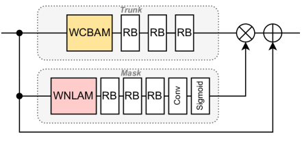
(a) Attention module with skip connection. RB denotes a residual block. WCBAM denotes a window-based convolutional block attention module and WNLAM is a window-based non-local attention module.

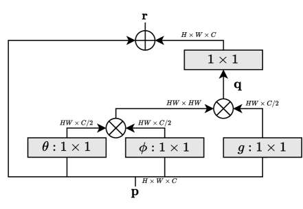
(b) Window-based non-local attention module (WNLAM).

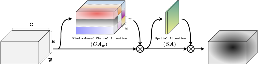
(c) Window-based convolutional block attention module (WCBAM). A feature map of C channels with spatial dimensions H$\times$W is the input to the WCBAM block. $w$ is the window size over which to calculate channel attention.

Figure 4: Attention module architecture.

3.2 Attention Assisted Image Compression

The attention mechanism in neural networks (discussed in Section 2.3) have been also employed in deep neural compression networks. (Zhou et al., 2019) applied residual attention, then (Chen et al., 2021) improved their work by adding a non-local attention mechanism to the mask of the residual attention. As a further improvement, (Zou et al., 2022) applied non-local attention limited to small windows of the feature maps. This window-based attention attained better results in compression. Here we propose to use two kinds of attention mechanisms in a window-based manner.

Solar images have a great amount of spatial redundancy compared to natural scene images. In this view, discarding the redundancy and only keeping the low frequency content, which is desired in natural image compression, could lead to high distortions unless paying the cost of transmitting high frequency contents as well. Another important issue when it comes to the compression of solar images is that the minute details and high frequency components are important for the analysis of data (for example solar flare detection and coronal hole segmentation), while in general image compression these high frequency details could be discarded without intolerable cost. To address these differences in the compression domain, we propose two separate attention mechanisms: First, to to apply a window-based non-local attention and second to refine features over a local window in the channel dimension enriching the latent code of the image.

3.2.1 Window-based Non-Local Attention Module (WNLAM)

To clarify the procedure of the window-based non-local attention mechanism, described in Section 2.3, a concise review of how this method enriches the representations learned by the convolutional neural networks is included in this section. A non-local attention block as shown in Fig. 4(b) is composed of a weighted average, denoted by $\mathbf{q}$, over a linear transformed version of the block input $\mathbf{p}$, i.e., $g(\mathbf{p})$:

$$\mathbf{q}_{i}=\frac{1}{\sum_{\forall j}e^{\theta(\mathbf{p}_{i})^{T}\phi(\mathbf{p}_{j})}}\sum_{\forall k}e^{\theta(\mathbf{p}_{i})^{T}\phi(\mathbf{p}_{k})}g(\mathbf{p}_{k}),$$ (15)

where $g(\cdot)$ is a linear transformation, with learnable parameters $W_{g}$ implemented by a $1\times 1$ convolution layer defined as $g(\mathbf{p_{k}})=W_{g}\mathbf{p_{k}}$. The weights of the sum in Eq. (15) are calculated by the measure of similarity in the embedding space of the input, i.e., $\theta(\mathbf{p}_{i})=W_{\theta}\mathbf{p_{i}}$ and $\phi(\mathbf{p}_{k})=W_{\phi}\mathbf{p_{k}}$, where $W_{\theta}$ and $W_{\phi}$ are learnable parameters.

As the final operation in non-local attention, $\mathbf{r}_{i}$ is calculated by a linear transformation ($W_{r}$) added to the original $\mathbf{p}_{i}$ as follows:

$$\mathbf{r}_{i}=W_{r}\mathbf{q}_{i}+\mathbf{p}_{i}.$$ (16)

Applying a non-local attention mechanism locally through non-overlapping windows has shown to be more effective in the task of image compression (Zou et al., 2022) than its global counterpart (Cheng et al., 2020). In high-bitrate image compression, restoring edges and high-frequency content is as important as representing the global features in the latent representation (Wallace, 1991; Ballé et al., 2018; Cheng et al., 2020). Consequently, a naïve non-local attention mechanism can perform worse than local attentions which are able to capture local redundancies and preserve details on the reconstructed image (Zou et al., 2022).

3.2.2 Window-based Convolutional Block Attention Module (WCBAM)

A simple to implement attention mechanism in CNNs is the convolutional block attention module (CBAM) which has shown great benefit in classification tasks (Woo et al., 2018). It includes two attention mechanisms. First, the channel attention ($CA$) guides the network to only consider channels with higher importance for the desired task. Second, the spatial attention ($SA$) dictates where the network should pay more attention. Here we propose to utilize this attention module in a window-based manner. Instead of globally considering the whole spatial extent of each channel, we focus only on a cropped window size of $w$, as shown in Fig. 4(c).

Applying the WCBAM mechanism on the input features $X$ can be summarized as:

$$X_{CA} =CA_{w}\odot X,$$ (17)

$$X_{CA,SA} =SA\odot X_{CA},$$

where $\odot$ is the Hadamard product. $CA_{w}$ reweighs the channels over each window. After refining the channels, the spatial attention enforces each of the refined channels ($X_{CA}$) to highlight their important spatial content for the task of image compression by the Hadamard product with $SA$.

The window-based channel attention is calculated by passing the average and max pool through a shared fully connected network ($F$), as in Eq. (18):

$$CA_{w}=sigmoid(F(Avg(X_{w}))+F(Max(X_{w}))),$$ (18)

where $X_{w}$ is a chosen window over the input feature map $X$. Next, the spatial attention weights ($SA$) will be derived by concatenating the average and max pool passed through a convolutional layer as:

$$SA=sigmoid(Conv([Avg(X_{CA}),Max(X_{CA})])).$$ (19)

WCBAM helps the network to capture global dependencies by looking over all channels of each chosen window simultaneously and highlighting the spatially important features with a global average/max pooled feature. These global features are needed in transforming the image from pixel space to feature space.

3.2.3 Transformers as Attention Modules

The superiority of models based on transformers, which are a special kind of non-local attention mechanism, compared to convolutional neural networks has been recently proven (Dosovitskiy et al., 2021; Liu et al., 2021). Although transformers have shown great benefit in image classification and object detection tasks, their naïve application in image compression networks has failed (Zou et al., 2022). The goal of transformers is to capture long-range dependencies in an image as opposed to convolutional-based neural networks which inherently have a local inductive bias due to the use of a local kernel. On the other hand, the ultimate goal of image compression is to capture both local and global dependencies in order to summarize them efficiently in the latent code. If the latent code includes global information, we can expect a more compact representation. By naïvely applying the transformer blocks in the neural compression networks, it was shown (Zou et al., 2022; Zhu et al., 2022) that optimizing the rate-distortion loss leads to a local receptive field, hindering the self-attention from global dependency modeling. Therefore enriching the attention mechanism in the convolutional neural networks, as we show in this work, could lead to better performance in terms of rate-distortion.

4 Experiments

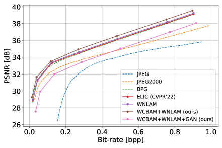
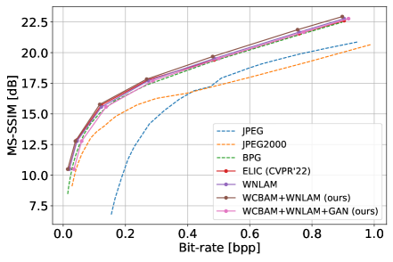
Figure 5: Rate-distortion curves averaged over the test set described in Section 4.1. On the left, PSNR is calculated from MSE using $10\log_{10}\frac{255^{2}}{MSE}$. On the right, MS-SSIM is reported in logarithmic scale by $-10\log(1-m)$ to show the differences better, in which $m$ is the MS-SSIM in the range of zero to one.

4.1 Dataset

The dataset of SDO images described in (Galvez et al., 2019) includes images of the sun at wavelengths of 94, 131, 171, 193, 211, 304, 335, 1600, and 1700 Å at a cadence of 6 minutes. We temporally downsampled the images to a cadence of 1 hour to decrease dependencies between training samples. In addition, to prevent biases of the images with respect to solar variations at different stages of the solar cycle, we followed the same approach proposed by (Salvatelli et al., 2019) to divide the dataset based on the month they are taken. Images from January to August of years 2015 to 2018 are chosen for training and September to December of the same years are reserved for testing. The total number of training images is 21,416 and the test set includes 8,257 samples. The results reported in this section are all based on the test portion of the dataset.

4.2 Implementation Details

As the nonlinearity in our neural network, we have utilized a computationally efficient (Johnston et al., 2019) version of Generalized Divisive Normalization (GDN) (Ballé et al., 2016b). As a result of GDN’s local normalization, statistical dependencies are reduced in the feature maps. By exploiting GDN instead of more conventional nonlinearities like ReLU, the statistical dependencies in the feature maps will be reduced significantly (Ballé et al., 2016b).

During the evaluation phase, entropy coding of the latent integer values was realized by range asymmetric numeral systems coding (Duda, 2013). It is worth mentioning that the entropy coding is lossless and doing it during the training phase has no impact on the measured performance or functionality of the algorithm. It is only during the evaluation phase that entropy coding is needed since the performance of algorithms is compared with standard codecs, such as JPEG (Wallace, 1991), JPEG-2000 (Taubman & Marcellin, 2002). Seven models have been trained with empirically chosen hyper-parameter $\lambda\in\displaystyle\{0.0015,0.0035,0.0070,0.0125,0.0250,0.0410,0.0550\}$ governing the rate-distortion trade-off as in Eq. (2) for 100 epochs. We have used the Adam (Kingma & Ba, 2015a) optimizer on batches of size 16 consisting of randomly cropped $256\times 256$ patches from the original $512\times 512$ images. The initial value of the learning rate is set to $10^{-4}$ and annealed during the training to $1.2\times 10^{-6}$ which took about 48 hours on a machine with a single NVIDIA RTX 6000A graphic card, for each model. In addition, to compare our proposed neural codec with state of the art neural-based codecs we picked ELIC (He et al., 2022) neural compression and trained with exactly the same hyper-parameters and training policies as described for our own networks.

Table 1: Encoding/decoding latency of the proposed neural-based codec compared other codecs in three different bitrate regimes (input image size of $4096\times 4096$ pixels). ENC and DEC refer to encoding and decoding times, respectively and are reported in milliseconds.

		$\sim 0.1$ bpp				$\sim 0.35$ bpp				$\sim 0.7$ bpp
Codec		ENC (ms)	DEC (ms)			ENC (ms)	DEC (ms)			ENC (ms)	DEC (ms)
JPEG (Wallace, 1991)		42	48			47	58			50	64
JPEG2000 (Taubman & Marcellin, 2002)		312	187			367	221			416	249
BPG (Bellard, 2018)		2340	2048			3032	2354			4080	2936
ELIC (He et al., 2022)		3671	3012			3754	3099			3818	3176
ours		3527	3321			3654	3423			3698	3455

Training our autoencoder based on MSE and LPIPS will result in outperforming even the state-of-the-art hand-engineered codec, i.e., BPG (Bellard, 2018), as shown in Fig. 5. As can be seen in this figure, augmenting the WNLAM attention with WCBAM is capable of improving the rate-distortion performance in terms of both distortion measures PSNR and MS-SSIM. Although the adversarially trained network with the GAN has a distortion performance almost the same as JPEG-2000 (Taubman & Marcellin, 2002), the general lower performance of our GAN network is a common issue addressed in (Blau & Michaeli, 2018). The PSNR or MS-SSIM are unable to capture the perceptual quality of the generated image in a GAN. The perceptual quality of GAN network reconstructions is discussed in Section 4.3, where the quality is measured by the perceptual metric LPIPS.

To evaluate our model’s computational complexity compared with other compression algorithms, we have conducted experiments to measure the encoding and decoding latencies as reported in Table 1. All hand-crafted codecs, including JPEG, JPEG2000, and BPG are evaluated on a system powered by Intel Core i7-5930K Broadwell-E CPU. Our proposed method and other state-of-the-art neural compression alogrithm (i.e., ELIC) are tested on a single NVIDIA RTX 6000A graphic card.

4.3 Ablation Study

To investigate how much the attention modules contribute to the performance of our neural compressor, we have trained three separate networks including a network with only the WNLAM module, then augmented with the WCBAM module, and finally augmented with the WCBAM module and trained adversarially in a GAN framework. Performance for each of the seven targeted bit-rates is discussed in Section 4.2. The first architecture has only the WNLAM module (Fig. 5) whose performance in terms of PSNR and MS-SSIM has been improved by adding the WCBAM attention module.

As emphasized in Fig. 1, the adversarially trained decoder results in better visual quality of the reconstructed image than the autoencoder only trained with the window-based non-local and convolutional block attention mechanisms. Conventional metrics like PSNR and MS-SSIM are unable to capture the higher perceptual quality of the GAN-reconstructed images. It is empirically shown (Zhang et al., 2018) that LPIPS can show the merit of an adversarially trained network. LPIPS is known as a measure of similarity between an image and its reconstruction and it is shown that it is consistent with the human judgment of the quality of reconstructed images (Zhang et al., 2018). As shown in Fig. 6, the adversarially trained network performs better than the others which are not trained using GANs. This figure shows that if the human judgment has priority over the PSNR/MS-SSIM, training adversarially is the best option.

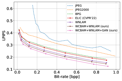
Figure 6: Rate-distortion curve. Distortion is measured by the LPIPS metric (lower is better) as described in Section 3.1.1. As shown, GAN performance in generating high-quality images can be quantified by this metric.

4.4 Example of the Impact on Downstream Use Applications

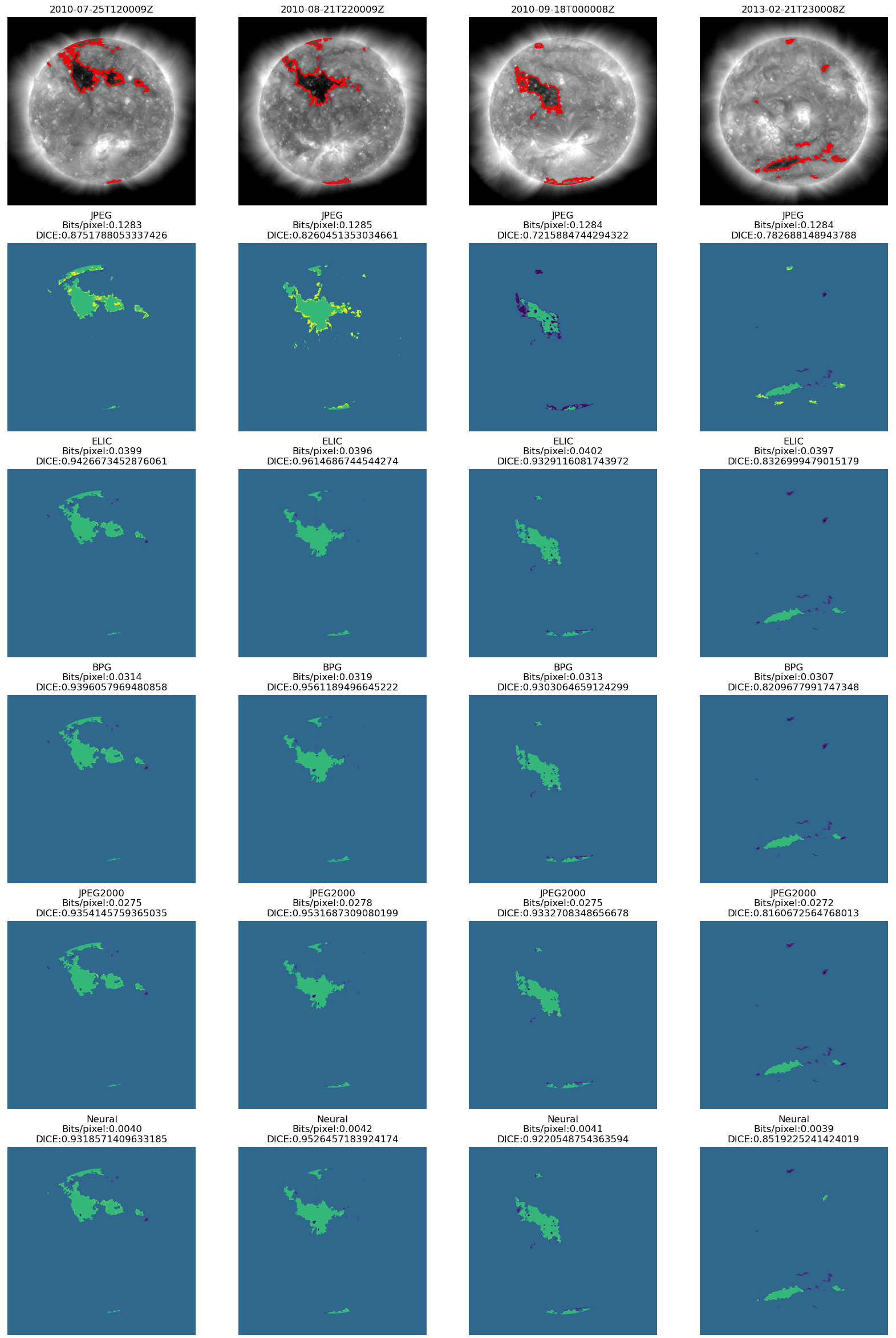
Figure 7: Effects of proposed compression scheme on CH detection via ACWE. The top row images are the original solar EUV images. At this wavelength CHs appear as dark regions. The CH segmentation on the original images is shown in the same row. The remaining images are comparisons of the original ACWE segmentation with the segmentation generated from the compressed images with different compression schemes. Last row contains the results of segmentation on reconstructed images through our proposed neural codec at sub $\sim 0.01$ bitrates, a bitrate regime not achievable by other codecs preserving the same DICE coefficient. In each image purple regions were only identified as CHs in the original segmentation, yellow regions were identified as belonging to a CH only in the compressed image segmentation, green regions were identified as CHs in both segmentations, and blue regions were not identified as CHs in either segmentation.

In order to provide an example of the effects of the proposed compression scheme on data science applications, the coronal hole (CH) detection and segmentation scheme outlined in Boucheron et al. (2016), which is an extension of the active contours without edges (ACWE) algorithm of Chan & Vese (2001), was applied to four 193 Å Solar EUV images. The effects of compression were determined by comparing the similarity of the resulting CH regions at various bit rates to the CH regions identified on the original Level 1 193 Å EUV images.

CHs are regions of low-density, low-temperature plasma within the Sun’s corona. These regions are associated with open magnetic field lines, and are sources of high-speed solar wind Altschuler et al. (1972); Munro & Withbroe (1972); Wang & Sheeley (1990); Wang et al. (1996). For this reason, accurate delineation of CH boundaries and extents is important for accurate space weather modeling and prediction Wang & Sheeley (1990); Arge et al. (2003; 2004). The segmentation scheme outlined in Boucheron et al. (2016) combines threshold-based detection, which is a common method of detecting CHs Reiss et al. (2021), with a region refinement algorithm that further refines the initial segmentation based on the homogeneity of the region. By using the algorithm of Boucheron et al. (2016) we can verify that region intensity and underlying structure necessary for accurate delineation of coronal holes are both preserved in the compressed images.

ACWE is an iterative process wherein an initial contour or ‘seed’ is manipulated on a pixel-by-pixel basis across multiple iterations in order to minimize an energy functional. The ACWE energy functional is minimized by balancing three forces which seek to 1: minimize the length of the contour, 2: maximize the homogeneity of the foreground (or CH region), and 3: maximize the homogeneity of the background or non-CH region Chan & Vese (2001). Each force is subject to a user-defined weight which defines the relative importance of achieving each goal Chan & Vese (2001). Unlike the process outlined in Boucheron et al. (2016), ACWE was performed on the images at the original resolution of $4096\times 4096$ pixels. The rest of the process follows the method outlined in Boucheron et al. (2016), wherein the images are corrected for limb brightening following the method outlined in Verbeeck et al. (2014). An initial seed is then generated by selecting all on-disk pixels with an intensity $\leq\alpha\times QS$ where $QS$ is the mean intensity of the quiet Sun, and the seeding parameter ($\alpha$) is defined as $\alpha=0.3$. From there ACWE was performed on the on-disk region using the length constraint $\mu=0$, and the ratio of foreground to background homogeneity parameters $\lambda_{i}/\lambda_{o}=50$.

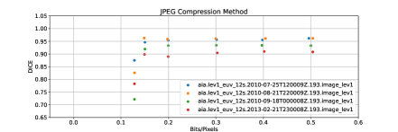
(a) JPEG

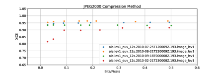
(b) JPEG-2000

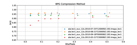
(c) BPG

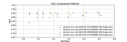
(d) ELIC

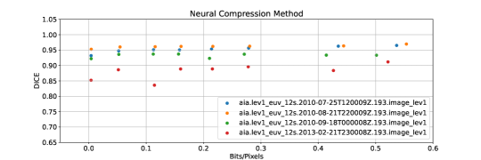
(e) Our Neural Codec

Figure 8: Effects of different compression schemes on CH detection via ACWE, expressed as DICE coefficient as a function of bit-rate.

The compression process was evaluated using four 193 Å Solar EUV images with record times (as expressed by the T_REC keyword) 2010-07-25 T12:00:02Z, 2010-08-21 T22:00:02Z, 2010-09-18 T00:00:02Z, and 2013-02-21 T23:00:01Z. In order to prepare the images for the compression process, the original Level 1 EUV image (at their native spatial resolution of $4096\times 4096$ pixels) were clipped to the intensity range of $[20,2500]$. Once clipped, a $\log_{10}$ transform was applied to the intensity levels within images. The resulting intensities where then mapped to 255 discrete levels before performing the compression using the proposed network (with both WNLAM and WCBAM attention). For this process eight models were developed using the hyper-parameters $\lambda=\{0.0005,0.0035,0.007,0.009,0.011,0.0125,0.019,0.025\}$. Once a compressed image for each EUV input was generated from each model, the images were then restored by reversing the intensity mapping and reversing the $\log_{10}$ transform prior to performing ACWE.

An example of the effects of the proposed compression scheme on the final CH segmentation is presented in Fig. 7. In this figure the output of compressed images by five different compression algorithms are compared, by showing the original image and its correct segmentation on the first row for four different images of the Sun. The subsequent rows are the highest compression rate achievable by the mentioned algorithm and as it can be seen the proposed neural compression method can still deliver in the sub-0.01 bpp regime. Each image in Fig. 7 is a comparison between the two segmentations (original and compressed) wherein purple regions were only identified as CHs in the original segmentation, yellow regions were identified as belonging to a CH only in the compressed image segmentation, green regions were identified as CHs in both segmentations, and blue regions were not identified as CHs in either segmentation. Within this image set, and the remaining cases tested, the discrepancies between segmentations are generally limited to small-scale structures, usually along the boundary of CH regions. This suggests that the proposed compression scheme is able to preserve the overall structure (and intensity) of coronal hole regions within the solar EUV image.

Across the four images, the effects of compression were evaluated by computing the DICE coefficient, defined as

$$DSC=\frac{2|S_{1}\cap S_{2}|}{|S_{1}|+|S_{2}|},$$ (20)

between the CH segmentation generated by ACWE from the original EUV image ($S_{1}$), and the segmentation generated from the compressed image ($S_{2}$), where $|\cdot|$ denotes cardinality and $\cap$ denotes intersection. These results, which are shown as a function of bit rate of the compressed image in Fig. 8, corroborates the observations seen in Fig. 7 by showing a high similarity between segmentations across all bit rates and more desirably in the extremely compressed regimes.

It should be noted that applying a log transformation to the intensities within an image increases the number of output intensity levels used to represent low intensities while decreasing the number of output levels used to represent high intensities. For this reason, more of the 255 discrete intensity levels were allocated to preserving fine detail at the low-intensity range of the image, which, in turn, improved the quality of the ACWE segmentation Grajeda et al. (2023).

To help disentangle the effects of this advantage, this same prepossessing was applied to the same EUV images before compressing the images using other compression, then reversing the process in the same manner. The DICE coefficient (again, compared to the segmentation of the original EUV image) as a function of the bit-rate of the compressed image for the other compression schemes is presented in Fig. 8. It should be noted that the other compression schemes begin to show signs of degradation in image features that negatively impact CH segmentation at compression rates of $\sim 0.12$ bits per pixel, and cannot produce images with a compression rate $<0.1$ bits per pixel for these 4K by 4K images, unless sacrificing DICE measure. One the other hand, the neural compression scheme proposed here continues to perform well beyond this threshold, suggesting that the neural compression scheme is able to better preserve the features that are relevant to this application.

5 Conclusion

In this work, we have shown how an effective image compression scheme based on trainable neural networks could be utilized for ad-hoc applications like images from NASA’s SDO mission. We explored the effectiveness of window-based spatial and cross-channel attention mechanisms in an adversarially trained neural network to improve the performance of compression in terms of rate-distortion-perception trade-off. It was shown that neural compression algorithms may be able to benefit data-intensive space missions with minimal degradation in downstream scientific tasks such as coronal hole segmentation as described in this work.

Acknowledgments

This research is based upon work supported by the National Aeronautics and Space Administration (NASA), via award number 80NSSC21M0322 under the title of Adaptive and Scalable Data Compression for Deep Space Data Transfer Applications using Deep Learning.

References

- Agustsson et al. (2017) Eirikur Agustsson, Fabian Mentzer, Michael Tschannen, Lukas Cavigelli, Radu Timofte, Luca Benini, and Luc Van Gool. Soft-to-hard vector quantization for end-to-end learning compressible representations. In Advances in Neural Information Processing, 2017.
- Agustsson et al. (2019) Eirikur Agustsson, Michael Tschannen, Fabian Mentzer, Radu Timofte, and Luc Van Gool. Generative adversarial networks for extreme learned image compression. In Proceedings of the IEEE/CVF International Conference on Computer Vision, 2019.
- Altschuler et al. (1972) Martin D. Altschuler, Dorothy E. Trotter, and Frank Q. Orrall. Coronal holes. Solar Physics, 26(2):354–365, October 1972. doi: 10.1007/BF00165276.
- Arge et al. (2004) C. N. Arge, J. G. Luhmann, D. Odstrcil, C. J. Schrijver, and Y. Li. Stream structure and coronal sources of the solar wind during the May 12th, 1997 CME. Journal of Atmospheric and Solar-Terrestrial Physics, 66(15-16):1295–1309, October 2004. doi: 10.1016/j.jastp.2004.03.018.
- Arge et al. (2003) Charles N. Arge, Dusan Odstrcil, Victor J. Pizzo, and Leslie R. Mayer. Improved method for specifying solar wind speed near the Sun. In Marco Velli, Roberto Bruno, Francesco Malara, and B. Bucci (eds.), Solar Wind Ten, volume 679 of American Institute of Physics Conference Series, pp. 190–193, September 2003. doi: 10.1063/1.1618574.
- Ballé et al. (2016a) Johannes Ballé, Valero Laparra, and Eero P. Simoncelli. End-to-end optimization of nonlinear transform codes for perceptual quality. In 2016 Picture Coding Symposium, PCS 2016. IEEE, 2016a.
- Ballé et al. (2016b) Johannes Ballé, Valero Laparra, and Eero P. Simoncelli. Density modeling of images using a generalized normalization transformation. In 4th International Conference on Learning Representations, 2016b.
- Ballé et al. (2017) Johannes Ballé, Valero Laparra, and Eero P. Simoncelli. End-to-end optimized image compression. In 5th International Conference on Learning Representations. OpenReview.net, 2017.
- Ballé et al. (2018) Johannes Ballé, David Minnen, Saurabh Singh, Sung Jin Hwang, and Nick Johnston. Variational image compression with a scale hyperprior. In 6th International Conference on Learning Representations, 2018.
- Ballé et al. (2021) Johannes Ballé, Philip A. Chou, David Minnen, Saurabh Singh, Nick Johnston, Eirikur Agustsson, Sung Jin Hwang, and George Toderici. Nonlinear transform coding. IEEE J. Sel. Top. Signal Process., 2021. doi: 10.1109/JSTSP.2020.3034501.
- Bellard (2018) Fabrice Bellard. Bpg image format. https://bellard.org/bpg/, 2018.
- Bishop (1999) Christopher M Bishop. Latent variable models. Learning in graphical models, 371, 1999.
- Bishop (2006) Christopher M Bishop. Pattern recognition and machine learning, volume 4. Springer, 2006.
- Blau & Michaeli (2018) Yochai Blau and Tomer Michaeli. The perception-distortion tradeoff. In 2018 IEEE Conference on Computer Vision and Pattern Recognition, CVPR 2018, Salt Lake City, UT, USA, June 18-22, 2018, pp. 6228–6237. Computer Vision Foundation / IEEE Computer Society, 2018. doi: 10.1109/CVPR.2018.00652.
- Blau & Michaeli (2019) Yochai Blau and Tomer Michaeli. Rethinking lossy compression: The rate-distortion-perception tradeoff. In International Conference on Machine Learning. PMLR, 2019.
- Boucheron et al. (2016) LE Boucheron, M Valluri, and RTJ McAteer. Segmentation of coronal holes using active contours without edges. Solar Physics, 291(8):2353–2372, 2016.
- Brock et al. (2019) Andrew Brock, Jeff Donahue, and Karen Simonyan. Large scale GAN training for high fidelity natural image synthesis. In 7th International Conference on Learning Representations, ICLR 2019, New Orleans, LA, USA, May 6-9, 2019. OpenReview.net, 2019. URL https://openreview.net/forum?id=B1xsqj09Fm.
- Buades et al. (2005) Antoni Buades, Bartomeu Coll, and J-M Morel. A non-local algorithm for image denoising. In 2005 IEEE Computer Society Conference on Computer Vision and Pattern Recognition (CVPR’05), volume 2. IEEE, 2005.
- Chan & Vese (2001) T.F. Chan and L.A. Vese. Active contours without edges. IEEE Transactions on Image Processing, 10(2):266–277, 2001. doi: 10.1109/83.902291.
- Chen et al. (2021) Tong Chen, Haojie Liu, Zhan Ma, Qiu Shen, Xun Cao, and Yao Wang. End-to-end learnt image compression via non-local attention optimization and improved context modeling. IEEE Transactions on Image Processing, 30, 2021.
- Cheng et al. (2020) Zhengxue Cheng, Heming Sun, Masaru Takeuchi, and Jiro Katto. Learned image compression with discretized gaussian mixture likelihoods and attention modules. In Proceedings of the IEEE Conference on Computer Vision and Pattern Recognition (CVPR), 2020.
- Cover (1999) Thomas M Cover. Elements of information theory. John Wiley & Sons, 1999.
- Dosovitskiy et al. (2021) Alexey Dosovitskiy, Lucas Beyer, Alexander Kolesnikov, Dirk Weissenborn, Xiaohua Zhai, Thomas Unterthiner, Mostafa Dehghani, Matthias Minderer, Georg Heigold, Sylvain Gelly, Jakob Uszkoreit, and Neil Houlsby. An image is worth 16x16 words: Transformers for image recognition at scale. In 9th International Conference on Learning Representations. OpenReview.net, 2021.
- Duda (2013) Jarek Duda. Asymmetric numeral systems: entropy coding combining speed of huffman coding with compression rate of arithmetic coding. arXiv preprint arXiv:1311.2540, 2013.
- Esser et al. (2021) Patrick Esser, Robin Rombach, and Bjorn Ommer. Taming transformers for high-resolution image synthesis. In Proceedings of the IEEE/CVF conference on computer vision and pattern recognition, pp. 12873–12883, 2021.
- Galvez et al. (2019) Richard Galvez, David F. Fouhey, Meng Jin, Alexandre Szenicer, Andrés Muñoz-Jaramillo, Mark C. M. Cheung, Paul J. Wright, Monica G. Bobra, Yang Liu, James Mason, and Rajat Thomas. A machine-learning data set prepared from the NASA solar dynamics observatory mission. The Astrophysical Journal Supplement Series, may 2019. doi: 10.3847/1538-4365/ab1005.
- Gersho & Gray (2012) Allen Gersho and Robert M Gray. Vector quantization and signal compression, volume 159. Springer Science & Business Media, 2012.
- Goodfellow et al. (2014) Ian Goodfellow, Jean Pouget-Abadie, Mehdi Mirza, Bing Xu, David Warde-Farley, Sherjil Ozair, Aaron Courville, and Yoshua Bengio. Generative adversarial nets. Advances in neural information processing systems, 2014.
- Goyal (2001) V.K. Goyal. Theoretical foundations of transform coding. IEEE Signal Processing Magazine, 18(5):9–21, 2001. doi: 10.1109/79.952802.
- Grajeda et al. (2023) J. A. Grajeda, L. E. Boucheron, M. S. Kirk, A. Leisner, and C. N. Arge. Quantifying the consistency and characterizing the confidence of coronal holes detected by active contours without edges (ACWE). Accepted: Solar Physics, 2023.
- Gray & Neuhoff (1998) Robert M. Gray and David L. Neuhoff. Quantization. IEEE Trans. Inf. Theory, 1998. doi: 10.1109/18.720541.
- Guo et al. (2021) Zongyu Guo, Zhizheng Zhang, Runsen Feng, and Zhibo Chen. Soft then hard: Rethinking the quantization in neural image compression. In International Conference on Machine Learning. PMLR, 2021.
- He et al. (2022) Dailan He, Ziming Yang, Weikun Peng, Rui Ma, Hongwei Qin, and Yan Wang. Elic: Efficient learned image compression with unevenly grouped space-channel contextual adaptive coding. In Proceedings of the IEEE/CVF Conference on Computer Vision and Pattern Recognition, pp. 5718–5727, 2022.
- He et al. (2016) Kaiming He, Xiangyu Zhang, Shaoqing Ren, and Jian Sun. Deep residual learning for image recognition. In Proceedings of the IEEE conference on computer vision and pattern recognition, 2016.
- Hu et al. (2018) Jie Hu, Li Shen, and Gang Sun. Squeeze-and-excitation networks. In Proceedings of the IEEE conference on computer vision and pattern recognition, 2018.
- Hu et al. (2022) Liwei Hu, Wenyong Wang, Yu Xiang, and Jun Zhang. Flow field reconstructions with gans based on radial basis functions. IEEE Transactions on Aerospace and Electronic Systems, 58(4):3460–3476, 2022.
- Isola et al. (2017) Phillip Isola, Jun-Yan Zhu, Tinghui Zhou, and Alexei A Efros. Image-to-image translation with conditional adversarial networks. In Proceedings of the IEEE conference on computer vision and pattern recognition, pp. 1125–1134, 2017.
- Johnston et al. (2019) Nick Johnston, Elad Eban, Ariel Gordon, and Johannes Ballé. Computationally efficient neural image compression. Technical report, Google Research, 2019.
- Jozdani et al. (2022) Shahab Jozdani, Dongmei Chen, Darren Pouliot, and Brian Alan Johnson. A review and meta-analysis of generative adversarial networks and their applications in remote sensing. International Journal of Applied Earth Observation and Geoinformation, 108:102734, 2022. ISSN 1569-8432. doi: https://doi.org/10.1016/j.jag.2022.102734. URL https://www.sciencedirect.com/science/article/pii/S0303243422000605.
- Karras et al. (2019) Tero Karras, Samuli Laine, and Timo Aila. A style-based generator architecture for generative adversarial networks. In Proceedings of the IEEE/CVF conference on computer vision and pattern recognition, pp. 4401–4410, 2019.
- Karras et al. (2020) Tero Karras, Samuli Laine, Miika Aittala, Janne Hellsten, Jaakko Lehtinen, and Timo Aila. Analyzing and improving the image quality of stylegan. In Proceedings of the IEEE/CVF conference on computer vision and pattern recognition, pp. 8110–8119, 2020.
- Kim et al. (2022) Jun-Hyuk Kim, Byeongho Heo, and Jong-Seok Lee. Joint global and local hierarchical priors for learned image compression. In Proceedings of the IEEE/CVF Conference on Computer Vision and Pattern Recognition, 2022.
- Kingma & Ba (2015a) Diederik P. Kingma and Jimmy Ba. Adam: A method for stochastic optimization. In 3rd International Conference on Learning Representations, 2015a.
- Kingma & Ba (2015b) Diederik P. Kingma and Jimmy Ba. Adam: A method for stochastic optimization. In 3rd International Conference on Learning Representations, 2015b.
- Ledig et al. (2017) Christian Ledig, Lucas Theis, Ferenc Huszár, Jose Caballero, Andrew Cunningham, Alejandro Acosta, Andrew Aitken, Alykhan Tejani, Johannes Totz, Zehan Wang, et al. Photo-realistic single image super-resolution using a generative adversarial network. In Proceedings of the IEEE conference on computer vision and pattern recognition, pp. 4681–4690, 2017.
- Lee et al. (2019) Jooyoung Lee, Seunghyun Cho, and Seung-Kwon Beack. Context-adaptive entropy model for end-to-end optimized image compression. In International Conference on Learning Representations, 2019.
- Li et al. (2021) Duo Li, Jie Hu, Changhu Wang, Xiangtai Li, Qi She, Lei Zhu, Tong Zhang, and Qifeng Chen. Involution: Inverting the inherence of convolution for visual recognition. In Proceedings of the IEEE/CVF Conference on Computer Vision and Pattern Recognition, pp. 12321–12330, 2021.
- Ling et al. (2021) Huan Ling, Karsten Kreis, Daiqing Li, Seung Wook Kim, Antonio Torralba, and Sanja Fidler. Editgan: High-precision semantic image editing. Advances in Neural Information Processing Systems, 34:16331–16345, 2021.
- Liu et al. (2022) Peng Liu, Jun Li, Lizhe Wang, and Guojin He. Remote sensing data fusion with generative adversarial networks: State-of-the-art methods and future research directions. IEEE Geoscience and Remote Sensing Magazine, 10(2):295–328, 2022. doi: 10.1109/MGRS.2022.3165967.
- Liu et al. (2021) Ze Liu, Yutong Lin, Yue Cao, Han Hu, Yixuan Wei, Zheng Zhang, Stephen Lin, and Baining Guo. Swin transformer: Hierarchical vision transformer using shifted windows. In ICCV. IEEE, 2021. doi: 10.1109/ICCV48922.2021.00986.
- Mentzer et al. (2020a) Fabian Mentzer, George D Toderici, Michael Tschannen, and Eirikur Agustsson. High-fidelity generative image compression. Advances in Neural Information Processing Systems, 33, 2020a.
- Mentzer et al. (2020b) Fabian Mentzer, George D Toderici, Michael Tschannen, and Eirikur Agustsson. High-fidelity generative image compression. Advances in Neural Information Processing Systems, 33:11913–11924, 2020b.
- Minnen & Singh (2020) David Minnen and Saurabh Singh. Channel-wise autoregressive entropy models for learned image compression. In IEEE International Conference on Image Processing, ICIP 2020, Abu Dhabi, United Arab Emirates, October 25-28, 2020, pp. 3339–3343. IEEE, 2020. doi: 10.1109/ICIP40778.2020.9190935.
- Minnen et al. (2018) David Minnen, Johannes Ballé, and George Toderici. Joint autoregressive and hierarchical priors for learned image compression. In Advances in Neural Information Processing, 2018.
- Munro & Withbroe (1972) Richard H. Munro and George L. Withbroe. Properties of a coronal “hole” derived from extreme-ultraviolet observations. The Astrophysical Journal, 176:511, September 1972. doi: 10.1086/151653.
- Nilsson & Akenine-Möller (2020) Jim Nilsson and Tomas Akenine-Möller. Understanding SSIM. arXiv preprint arXiv:2006.13846, 2020.
- Poirier-Ginter & Lalonde (2023) Yohan Poirier-Ginter and Jean-François Lalonde. Robust unsupervised stylegan image restoration. In Proceedings of the IEEE/CVF Conference on Computer Vision and Pattern Recognition, pp. 22292–22301, 2023.
- Qian et al. (2021) Yichen Qian, Zhiyu Tan, Xiuyu Sun, Ming Lin, Dongyang Li, Zhenhong Sun, Hao Li, and Rong Jin. Learning accurate entropy model with global reference for image compression. In International Conference on Learning Representations, 2021.
- Qian et al. (2022) Yichen Qian, Xiuyu Sun, Ming Lin, Zhiyu Tan, and Rong Jin. Entroformer: A transformer-based entropy model for learned image compression. In International Conference on Learning Representations, 2022.
- Rahman et al. (2022) Mohammed Mahbubur Rahman, Sevgi Z Gurbuz, and Moeness G Amin. Physics-aware generative adversarial networks for radar-based human activity recognition. IEEE Transactions on Aerospace and Electronic Systems, 2022.
- Ramachandran et al. (2019) Prajit Ramachandran, Niki Parmarand, Ashish Vaswani, Irwan Bello, Anselm Levskaya, and Jonathon Shlens. Stand-alone self-attention in vision models. In Advances in Neural Information Processing, 2019.
- Reiss et al. (2021) Martin A. Reiss, Karin Muglach, Christian Möstl, Charles N. Arge, Rachel Bailey, Véronique Delouille, Tadhg M. Garton, Amr Hamada, Stefan Hofmeister, Egor Illarionov, Robert Jarolim, Michael S. F. Kirk, Alexander Kosovichev, Larisza Krista, Sangwoo Lee, Chris Lowder, Peter J. MacNeice, and Astrid Veronig. The observational uncertainty of coronal hole boundaries in automated detection schemes. The Astrophysical Journal, 913(1):28, May 2021. ISSN 1538-4357. doi: 10.3847/1538-4357/abf2c8. URL http://dx.doi.org/10.3847/1538-4357/abf2c8.
- Salvatelli et al. (2019) Valentina Salvatelli, Souvik Bose, Brad Neuberg, Luiz FG dos Santos, Mark Cheung, Miho Janvier, Atilim Gunes Baydin, Yarin Gal, and Meng Jin. Using U-Nets to create high-fidelity virtual observations of the solar corona. Advances in Neural Information Processing Systems, 32, 2019.
- Taubman & Marcellin (2002) David S. Taubman and Michael W. Marcellin. JPEG2000 - image compression fundamentals, standards and practice. The Kluwer international series in engineering and computer science. Kluwer, 2002. doi: 10.1007/978-1-4615-0799-4.
- Theis et al. (2016) L. Theis, A. van den Oord, and M. Bethge. A note on the evaluation of generative models. In International Conference on Learning Representations, 2016.
- Theis et al. (2017) Lucas Theis, Wenzhe Shi, Andrew Cunningham, and Ferenc Huszár. Lossy image compression with compressive autoencoders. In 5th International Conference on Learning Representations. OpenReview.net, 2017.
- Toner & Fletcher (2022) Nathan Toner and Justin Fletcher. Self-attending task generative adversarial network for realistic satellite image creation. In 2022 IEEE Aerospace Conference (AERO), pp. 1–9. IEEE, 2022.
- Van den Oord et al. (2016) Aaron Van den Oord, Nal Kalchbrenner, Lasse Espeholt, Oriol Vinyals, Alex Graves, et al. Conditional image generation with pixelcnn decoders. Advances in neural information processing systems, 29, 2016.
- Verbeeck et al. (2014) C. Verbeeck, V. Delouille, B. Mampaey, and R. De Visscher. The SPoCA-suite: Software for extraction, characterization, and tracking of active regions and coronal holes on EUV images. Astronomy & Astrophysics, 561:A29, 2014. doi: 10.1051/0004-6361/201321243. URL https://doi.org/10.1051/0004-6361/201321243.
- Wallace (1991) Gregory K. Wallace. The JPEG still picture compression standard. Commun. ACM, 1991. doi: 10.1145/103085.103089.
- Wang et al. (2017) Fei Wang, Mengqing Jiang, Chen Qian, Shuo Yang, Cheng Li, Honggang Zhang, Xiaogang Wang, and Xiaoou Tang. Residual attention network for image classification. In CVPR, pp. 3156–3164, 2017.
- Wang et al. (2018) Xiaolong Wang, Ross Girshick, Abhinav Gupta, and Kaiming He. Non-local neural networks. In Proceedings of the IEEE conference on computer vision and pattern recognition, 2018.
- Wang & Sheeley (1990) Y. M. Wang and Jr. Sheeley, N. R. Solar wind speed and coronal flux-tube expansion. The Astrophysical Journal, 355:726, June 1990. doi: 10.1086/168805.
- Wang et al. (1996) Yi-Ming Wang, Scott H. Hawley, and Jr. Sheeley, Neil R. The magnetic nature of coronal holes. Science, 271(5248):464–469, January 1996. doi: 10.1126/science.271.5248.464.
- Wang & Bovik (2009) Zhou Wang and Alan C Bovik. Mean squared error: Love it or leave it? a new look at signal fidelity measures. IEEE signal processing magazine, 2009.
- Wang et al. (2023) Zi Wang, Minglin Chen, Yulan Guo, Zhang Li, and Qifeng Yu. Bridging the domain gap in satellite pose estimation: a self-training approach based on geometrical constraints. IEEE Transactions on Aerospace and Electronic Systems, 2023.
- Woo et al. (2018) Sanghyun Woo, Jongchan Park, Joon-Young Lee, and In So Kweon. CBAM: Convolutional block attention module. In Proceedings of the European conference on computer vision (ECCV), 2018.
- Xiao et al. (2015) Tianjun Xiao, Yichong Xu, Kuiyuan Yang, Jiaxing Zhang, Yuxin Peng, and Zheng Zhang. The application of two-level attention models in deep convolutional neural network for fine-grained image classification. In Proceedings of the IEEE conference on computer vision and pattern recognition, pp. 842–850, 2015.
- Yang et al. (2020) Yibo Yang, Robert Bamler, and Stephan Mandt. Variational bayesian quantization. In International Conference on Machine Learning. PMLR, 2020.
- Yang et al. (2022) Yibo Yang, Stephan Mandt, and Lucas Theis. An introduction to neural data compression. CoRR, abs/2202.06533, 2022.
- Zafari et al. (2022) Ali Zafari, Atefeh Khoshkhahtinat, Piyush M. Mehta, Nasser M. Nasrabadi, Barbara J. Thompson, Daniel Da Silva, and Michael S. F. Kirk. Attention-based generative neural image compression on solar dynamics observatory. In 2022 21st IEEE International Conference on Machine Learning and Applications (ICMLA), pp. 198–205, 2022. doi: 10.1109/ICMLA55696.2022.00035.
- Zhang et al. (2018) Richard Zhang, Phillip Isola, Alexei A Efros, Eli Shechtman, and Oliver Wang. The unreasonable effectiveness of deep features as a perceptual metric. In CVPR, 2018.
- Zhang et al. (2019) Yulun Zhang, Kunpeng Li, Kai Li, Bineng Zhong, and Yun Fu. Residual non-local attention networks for image restoration. In International Conference on Learning Representations, 2019.
- Zhao et al. (2017) Hang Zhao, Orazio Gallo, Iuri Frosio, and Jan Kautz. Loss functions for image restoration with neural networks. IEEE Trans. Computational Imaging, 2017. doi: 10.1109/TCI.2016.2644865.
- Zhou et al. (2021) Jingkai Zhou, Varun Jampani, Zhixiong Pi, Qiong Liu, and Ming-Hsuan Yang. Decoupled dynamic filter networks. In Proceedings of the IEEE/CVF Conference on Computer Vision and Pattern Recognition, pp. 6647–6656, 2021.
- Zhou et al. (2019) Lei Zhou, Zhenhong Sun, Xiangji Wu, and Junmin Wu. End-to-end optimized image compression with attention mechanism. In CVPR Workshops, June 2019.
- Zhu et al. (2017) Jun-Yan Zhu, Taesung Park, Phillip Isola, and Alexei A Efros. Unpaired image-to-image translation using cycle-consistent adversarial networks. In Proceedings of the IEEE international conference on computer vision, pp. 2223–2232, 2017.
- Zhu et al. (2022) Yinhao Zhu, Yang Yang, and Taco Cohen. Transformer-based transform coding. In International Conference on Learning Representations, 2022. URL https://openreview.net/forum?id=IDwN6xjHnK8.
- Zou et al. (2022) Renjie Zou, Chunfeng Song, and Zhaoxiang Zhang. The devil is in the details: Window-based attention for image compression. In CVPR, 2022.