A distributed multi-GPU ab initio density matrix renormalization group algorithm with applications to the P-cluster of nitrogenase

Abstract

The presence of many degenerate $d/f$ orbitals makes polynuclear transition metal compounds such as iron-sulfur clusters in nitrogenase challenging for state-of-the-art quantum chemistry methods. To address this challenge, we present the first distributed multi-GPU (Graphics Processing Unit) ab initio density matrix renormalization (DMRG) algorithm, suitable for modern high-performance computing (HPC) infrastructures. The central idea is to parallelize the most computationally intensive part - the multiplication of $O(K^{2})$ operators with a trial wavefunction, where $K$ is the number of spatial orbitals, by combining operator parallelism for distributing the workload with a batched algorithm for performing contractions on GPU. With this new implementation, we are able to reach an unprecedentedly large bond dimension $D=14000$ on 48 GPUs (NVIDIA A100 80 GB SXM) for an active space model (114 electrons in 73 active orbitals) of the P-cluster, which is nearly three times larger than the bond dimensions reported in previous DMRG calculations for the same system using only CPUs.

University of Chinese Academy of Sciences, Beijing, China

1 Introduction

The density matrix renormalization group (DMRG) algorithm^{1, 2} is a powerful numerical tool initially invented for computational study of strongly correlated one-dimensional systems. Its adaptation to quantum chemistry often referred as ab initio DMRG^{3, 4, 5, 6, 7, 8, 9, 10, 11, 12, 13, 14, 15, 16, 17, 18, 19, 20, 21, 22, 23, 24, 25, 26, 27, 28, 29, 30, 31, 32, 33, 34, 35, 36, 37, 38}. has made the study of transition metal complexes with several metal centers become possible, where the traditional full configuration interaction (FCI) is usually limited to one or two transition metal centers. Typical examples include the applications to the oxygen-evolving complex²⁷ [Mn4CaO5], the iron-sulfur clusters with [Fe2S2] and [Fe4S4] cores²⁸, the P-cluster [Fe8S7] and FeMoco [Fe7MoS9C] of nitrogenase with eight transition metal centers^{39, 40, 41}. It should be emphasized that the entanglement structure between orbitals in these molecules is more complex than that in one-dimensional systems. As a result, while for one-dimensional systems the ground state can be well captured by a finite bond dimension $D$ in the underlying variational wavefunction, independent of the system size⁴², the variational energy as a function of the bond dimension $D$ converges much more slowly for these complicated systems. This means that the bond dimension required to reach certain accuracy (e.g. 1 milli-Hartree per metal) for these systems needs to increase as the system size increases. In view of the computational scaling of ab initio DMRG, which is $O(K^{3}D^{3}+K^{4}D^{2})$ with $K$ being the number of spatial orbitals, this presents a huge computational challenge, which limits the typical value of $D$ to several thousands.

In view of such challenges, the major goal of the present work is to develop a new parallelization algorithm for ab initio DMRG, which can take advantage of modern heterogeneous high-performance computing (HPC) infrastructures. To date, Graphics Processing Unit (GPU) has become the most common accelerating device in HPC systems, for example, seven of the top ten supercomputers on the top 500 list ⁴³ are equipped with GPUs. The many-core architecture of GPU is specially designed for compute-bound and memory-bound tasks such as matrix-matrix multiplication (GEMM) and fast Fourier transformation (FFT), respectively. As a result, GPU has been widely adopted in computational chemistry and physics packages, e.g., TeraChem ^{44, 45}, GAMESS⁴⁶, FermiONs++⁴⁷, VASP ^{48, 49}, PWmat ^{50, 51}, Quantum Espresso ⁵², BerkeleyGW ⁵³, etc. In addition, recent developments of Tensor Cores ⁵⁴ have significantly improved the computational capability of GPUs, in particular, GEMM in double precision can be further accelerated on NVIDIA A100 or H100 GPUs.

Effectively utilizing the power of modern heterogeneous HPC infrastructures is nontrivial for ab initio DMRG, whose parallelization is less straightforward due to the complexity of the algorithm itself and the data structure involved. Different parallelization strategies need to be combined to achieve good performance. The first parallelization strategy developed by Chan¹⁰, which will be referred as operator parallelism, is based on a partition of normal/complementary operators. It can distribute the computation as well as the memory and disk requirements across different nodes. When symmetry is used, the matrix representation of operators becomes block-sparse. Based on this, Kurashige and Yanai⁵⁵ developed a parallelization strategy by distributing symmetry sectors. Li and Chan⁵⁶ realized the parallelization based on the sum of matrix product operators (MPO) representation⁵⁷ for the Hamiltonian in the context of spin-projected DMRG. Brabec et al.⁵⁸ combined operator and symmetry sector parallelisms and applied the resulting program to the FeMoco cluster (with an active space comprising 113 electrons in 76 orbitals⁴⁰) with a bond dimension equal to 6000 using approximately 2000 CPU cores. Zhai et al.⁵⁹ combined the real-space⁶⁰ and the sum of MPO⁵⁷ parallelisms and achieved a good parallel scaling up to thousands of CPU cores. The development of heterogeneous parallel strategy for ab initio DMRG appears only very recently. Menczer and Legeza^{61, 62} reported a single-node multi-GPU parallelization of ab initio DMRG and applied to the FeMoco with $D=4096$⁶². Apart from these parallelization strategies developed for ab initio DMRG, other parallelization strategies have also been introduced in the context of DMRG for model Hamiltonians^{63, 64, 65, 66, 67, 68, 69, 70}. A closely related work to the present study is the application of batched GEMM on GPU using the MAGMA⁷¹ library in the DMRG++ code⁶⁶. For a review of previous parallel DMRG studies, see Ref. ⁷². To the best of our knowledge, distributed multi-GPU parallelization of ab initio DMRG has not been reported.

In this work, we present a distributed multi-GPU ab initio DMRG algorithm. The central idea is to perform the most computationally intensive part, that is, the multiplication of $O(K^{2})$ operators with a trial wavefunction, by combining operator parallelism for distributing the workload with a batched algorithm for performing contractions on GPU. The remainder of the paper is organized as follows. In Sec. 2, we recapitulate DMRG and introduce our distributed multi-GPU parallelization. In Sec. 3, we benchmark the algorithm by applying it to the ground-state energy of an active space model (114 electrons in 73 active orbitals) of the P-cluster³⁹ and analyze the performance of our implementation. The capability of the present algorithm is demonstrated by reaching an unprecedentedly large bond dimension $D=14000$ for the P-cluster model, which is nearly three times larger than the bond dimensions reported in previous DMRG calculations for the same system using only CPUs. Conclusions and outlooks for future directions are presented in Sec. 4.

2 Theory and algorithm

2.1 Recapitulation of DMRG

The DMRG algorithm is a variational algorithm aiming to find the low-lying eigenstate of a Hamiltonian

$$\hat{H}\Psi=E\Psi,$$ (1)

with

$$\hat{H}=\sum_{pq}h_{pq}\hat{a}_{p}^{\dagger}\hat{a}_{q}+\frac{1}{4}\sum_{pqrs}\langle pq\|rs\rangle\hat{a}_{p}^{\dagger}\hat{a}_{q}^{\dagger}\hat{a}_{s}\hat{a}_{r},$$ (2)

by a special low-rank approximation, called matrix product states^{73, 57} (MPS), where the many-body wavefunction $\Psi$ in the Fock space is approximated as

$$\Psi^{n_{1}n_{2}\cdots n_{K}}\approx\sum_{\{\alpha_{k}\}}A^{n_{1}}_{\alpha_{1}}[1]A^{n_{2}}_{\alpha_{1}\alpha_{2}}[2]\cdots A^{n_{k}}_{\alpha_{k-1}\alpha_{k}}[k]\cdots A^{n_{K}}_{\alpha_{K-1}}[K],$$ (3)

with $n_{k}\in\{0,1,2,3\}$ for the occupation patterns $\{|vac\rangle,|k_{\beta}\rangle,|k_{\alpha}\rangle,|k_{\alpha}k_{\beta}\rangle\}$. Here, the tensors at the boundary $A^{n_{1}}_{\alpha_{1}}[1]$ and $A^{n_{K}}_{\alpha_{K-1}}[K]$ are matrices, while those $A^{n_{k}}_{\alpha_{k-1}\alpha_{k}}[k]$ in the middle of the MPS chain are rank-3 tensors. In practice, a maximal value $D$ for the virtual index $\alpha_{k}$ is given as an input for the DMRG algorithm. It is usually referred as the bond dimension, and controls the accuracy of the DMRG calculations. The set of tensors $\{A^{n_{k}}_{\alpha_{k-1}\alpha_{k}}[k]\}$ is to be found by minimizing the energy function

$$E[\{A^{n_{k}}_{\alpha_{k-1}\alpha_{k}}[k]\}]=\langle\Psi(\{A^{n_{k}}_{\alpha_{k-1}\alpha_{k}}[k]\})|\hat{H}|\Psi(\{A^{n_{k}}_{\alpha_{k-1}\alpha_{k}}[k]\})\rangle,$$ (4)

subject to the normalization condition $\langle\Psi(\{A^{n_{k}}_{\alpha_{k-1}\alpha_{k}}[k]\})|\Psi(\{A^{n_{k}}_{\alpha_{k-1}\alpha_{k}}[k]\})\rangle=1$. Since the number of parameters in each tensor $A^{n_{k}}_{\alpha_{k-1}\alpha_{k}}[k]$ scales as $O(D^{2})$, the total of parameters in an MPS is of $O(KD^{2})$. In DMRG, the optimization is carried out in a sequential way (called sweep), in which all other tensors are kept fixed when a one-site tensor $C^{n_{k}}_{\alpha_{k-1}\alpha_{k}}[k]$ or a two-site tensor $C^{n_{k}n_{k+1}}_{\alpha_{k-1}\alpha_{k+1}}[k,k+1]\triangleq(A[k]A[k+1])^{n_{k}n_{k+1}}_{\alpha_{k-1}\alpha_{k+1}}$ is being optimized in one-dot or two-dot sweep algorithms.

In the commonly used two-dot algorithm, Eq. (1) is solved in a direct product space $V_{L}\otimes V_{C_{1}}\otimes V_{C_{2}}\otimes V_{R}=\{|l_{k-1}n_{k}n_{k+1}r_{k+1}\rangle\}$, which is a subspace of the entire Fock space defined by the contracted basis $|l_{k-1}n_{k}n_{k+1}r_{k+1}\rangle$, using an iterative algorithm such as the Davidson algorithm⁷⁴. In this case, the Hamiltonian $\hat{H}$ (2) can be written as a sum of product form

$$\hat{H}=\sum_{\mu}\hat{O}^{L}_{\mu}\hat{O}^{C_{1}}_{\mu}\hat{O}^{C_{2}}_{\mu}\hat{O}^{R}_{\mu}.$$ (5)

where the number of terms ($\mu$) scales as $O(K^{2})$ for the second-quantized ab initio Hamiltonian^{3, 6}. The wavefunction expanded in this space reads

$$|\Psi\rangle=\sum_{lc_{1}c_{2}r}|lc_{1}c_{2}r\rangle\Psi^{lc_{1}c_{2}r}.$$ (6)

In the DMRG algorithm, the Hamiltonian-wavefunction multiplication is usually the most time-consuming part, i.e.

$$\sigma^{l^{\prime}c_{1}^{\prime}c_{2}^{\prime}r^{\prime}} = \sum_{\mu}\sum_{lc_{1}c_{2}r}\langle l^{\prime}c_{1}^{\prime}c_{2}^{\prime}r^{\prime}|\hat{O}^{L}_{\mu}\hat{O}^{C_{1}}_{\mu}\hat{O}^{C_{2}}_{\mu}\hat{O}^{R}_{\mu}|lc_{1}c_{2}r\rangle\Psi^{lc_{1}c_{2}r}$$ (7)

$$= \sum_{\mu}\sum_{lc_{1}c_{2}r}\zeta_{\mu lc_{1}c_{2}}[\hat{O}^{L}_{\mu}]_{l^{\prime}l}[\hat{O}^{C_{1}}_{\mu}]_{c_{1}^{\prime}c_{1}}[\hat{O}^{C_{2}}_{\mu}]_{c_{2}^{\prime}c_{2}}[\hat{O}^{R}_{\mu}]_{r^{\prime}r}\Psi^{lc_{1}c_{2}r},$$

where $\zeta_{\mu lc_{1}c_{2}}$ is a factor ($\pm 1$) due to the Fermionic character of electrons. The dimensions of $\hat{O}^{C_{1}}$ and $\hat{O}^{C_{2}}$ are 4, while the dimensions of $\hat{O}^{L}$ and $\hat{O}^{R}$ are $D$. Therefore, the computational cost for Eq. (7) scales as $O(K^{2}D^{3})$, and hence the total cost per sweep is $O(K^{3}D^{3})$. After a new wavefunction $\Psi^{lc_{1}c_{2}r}$ is obtained in the Davidson step, the site tensor $A[k]$ can be updated using singular value decomposition (SVD) or diagonalizing the reduced density matrix¹. This is referred to as the decimation step. With the new $A[k]$, a renormalization step is performed to produce the updated $\hat{O}^{L}$ or $\hat{O}^{R}$ for the next cycle, e.g.

$$[\hat{O}^{\mathrm{new}}_{\mu}]_{r^{\prime}r}=\sum_{l^{\prime}c^{\prime}}\sum_{lc}A_{l^{\prime}r^{\prime}}^{c^{\prime}*}\langle l^{\prime}c^{\prime}|\hat{O}^{L}_{\mu}\hat{O}^{C}_{\mu}|lc\rangle A_{lr}^{c}=\sum_{l^{\prime}c^{\prime}}\sum_{lc}\zeta_{\mu l}A_{l^{\prime}r^{\prime}}^{c^{\prime}*}[\hat{O}^{L}_{\mu}]_{l^{\prime}l}[\hat{O}^{C}_{\mu}]_{c^{\prime}c}A_{lr}^{c},$$ (8)

which scales also as $O(K^{3}D^{3})$ per sweep. For a more detailed description of the DMRG algorithm, the reader is referred to Ref. ⁶.

2.2 Distributed multi-GPU parallelization

The distributed parallelization algorithm by Chan¹⁰ distributes the computation of Eq. (7) by distributing $\mu$ (corresponding to contraction pairs of normal and complementary operators⁶) to different processors at the cost of replicating creation/annihilation operators and communications of complementary operators ($\hat{S}_{p}$ and $\hat{H}$) using the message passing interface (MPI)⁷⁵. The leading computational cost for the Davidson and renormalization steps becomes $O([K^{3}D^{3}+K^{4}D^{2}]/n_{p})$ with $n_{p}$ being the number of processors¹⁰. In this work, we use this algorithm to distribute operators and partition $\mu$ to different processes on difference nodes. Furthermore, we assume that a GPU is bound to a process, and we will use GPU to accelerate the contractions in Eqs. (7) and (8) for each process.

In this work, we use Abelian symmetries in DMRG to reduce the computational cost and memory consumption. Consequently, the operators are block-sparse and only the nonzero blocks are stored, see Fig. 1. We will use capital letters to represent symmetry blocks. In the Davidson diagonalization step, we implementation Eq. (7) via eight (instead of four as some operators are Hermitian conjugate of basic operators) batches of contractions at the level of symmetry blocks, viz.

$$I^{0/1}_{\mu L^{\prime}R^{\prime}C_{1}^{\prime}C_{2}^{\prime}LRC_{1}C_{2}}(LRC_{1}C_{2}^{\prime}) = [\hat{O}_{\mu}]_{C_{2}^{\prime}C_{2}}\cdot\Psi(LRC_{1}C_{2}),$$ (9)

$$I^{2/3}_{\mu L^{\prime}R^{\prime}C_{1}^{\prime}C_{2}^{\prime}LRC_{1}C_{2}}(LRC_{1}^{\prime}C_{2}^{\prime}) = [\hat{O}_{\mu}]_{C_{1}^{\prime}C_{1}}\cdot I^{0/1}_{\mu L^{\prime}R^{\prime}C_{1}^{\prime}C_{2}^{\prime}LRC_{1}C_{2}}(LRC_{1}C_{2}^{\prime}),$$ (10)

$$I^{4/5}_{\mu L^{\prime}R^{\prime}C_{1}^{\prime}C_{2}^{\prime}LRC_{1}C_{2}}(LR^{\prime}C_{1}^{\prime}C_{2}^{\prime}) = [\hat{O}_{\mu}]_{R^{\prime}R}\cdot I^{2/3}_{\mu L^{\prime}R^{\prime}C_{1}^{\prime}C_{2}^{\prime}LRC_{1}C_{2}}(LRC_{1}^{\prime}C_{2}^{\prime}),$$ (11)

$$I^{6/7}_{\mu L^{\prime}R^{\prime}C_{1}^{\prime}C_{2}^{\prime}LRC_{1}C_{2}}(L^{\prime}R^{\prime}C_{1}^{\prime}C_{2}^{\prime}) = [\hat{O}_{\mu}]_{L^{\prime}L}\cdot I^{4/5}_{\mu L^{\prime}R^{\prime}C_{1}^{\prime}C_{2}^{\prime}LRC_{1}C_{2}}(LR^{\prime}C_{1}^{\prime}C_{2}^{\prime}),$$ (12)

$$\sigma(L^{\prime}R^{\prime}C_{1}^{\prime}C_{2}^{\prime}) = \sum_{\mu}\sum_{LRC_{1}C_{2}}\zeta_{\mu LC_{1}C_{2}}\cdot I^{6/7}_{\mu L^{\prime}R^{\prime}C_{1}^{\prime}C_{2}^{\prime}LRC_{1}C_{2}}(L^{\prime}R^{\prime}C_{1}^{\prime}C_{2}^{\prime}),$$ (13)

where $\sigma(L^{\prime}R^{\prime}C_{1}^{\prime}C_{2}^{\prime})$ represents the symmetry block of $\sigma^{lc_{1}c_{2}r}$ (7) stored in C order, and the subscript in $I_{\mu L^{\prime}R^{\prime}C_{1}^{\prime}C_{2}^{\prime}LRC_{1}C_{2}}$ indicates that the intermediate is obtained from the term $\mu$ and the combination of symmetry blocks $L^{\prime}R^{\prime}C_{1}^{\prime}C_{2}^{\prime}$ and $LRC_{1}C_{2}$. For nonrelativistic or spin-free scalar relativistic Hamiltonians with particle number and spin projection symmetry, $[\hat{O}_{\mu}]_{C_{1}^{\prime}C_{1}}$ and $[\hat{O}_{\mu}]_{C_{2}^{\prime}C_{2}}$ are just numbers, and hence Eqs. (9) and (10) can be omitted by absorbing these factors into the scalar factor in the final step (13). For relativistic Hamiltonian including spin-orbit couplings, the spin projection is no longer a good quantum number, and $[\hat{O}_{\mu}]_{C_{1}^{\prime}C_{1}}$ and $[\hat{O}_{\mu}]_{C_{2}^{\prime}C_{2}}$ can be either a scalar or a two-by-two matrix. In this case, all the eight batches of contractions are needed. Each batch of contractions in Eqs. (9)-(12) can be recast into a batch of independent dense matrix-matrix multiplications (see Fig. 1). The preprocessing of different terms in the Hamiltonian ($\mu$), symmetry blocks (i.e., $L$, $R$, etc.), and the expansion of Eqs. (9)-(12) into dense matrix-matrix multiplications are carried out on CPU. Each batch of matrix multiplications takes the form

$$\{\mathbf{C}_{1}=\mathbf{A}_{1}\mathbf{B}_{1},\;\cdots,\;\mathbf{C}_{T}=\mathbf{A}_{T}\mathbf{B}_{T}\}.$$ (14)

However, the dimensions of the matrices are not the same, and its efficient computation using batched GEMM on GPU will be discussed in details in the next section. A similar strategy is developed for the renormalization step (8), viz.

$$I_{\mu L^{\prime}R^{\prime}C^{\prime}LRC}^{0/1}(LRC^{\prime}) = [\hat{O}^{C}_{\mu}]_{C^{\prime}C}\cdot A(LRC),$$ (15)

$$I_{\mu L^{\prime}R^{\prime}C^{\prime}LRC}^{2/3}(L^{\prime}RC^{\prime}) = [\hat{O}^{L}_{\mu}]_{L^{\prime}L}\cdot I_{\mu L^{\prime}R^{\prime}C^{\prime}LRC}^{0/1}(LRC^{\prime}),$$ (16)

$$I_{\mu L^{\prime}R^{\prime}C^{\prime}LRC}^{4}(R^{\prime}R) = A^{*}(L^{\prime}R^{\prime}C^{\prime})\cdot I_{\mu L^{\prime}R^{\prime}C^{\prime}LRC}^{2/3}(L^{\prime}RC^{\prime}),$$ (17)

$$[\hat{O}^{\mathrm{new}}_{\mu}]_{R^{\prime}R} = \sum_{L^{\prime}C^{\prime}LC}\zeta_{\mu L}\cdot I_{\mu L^{\prime}R^{\prime}C^{\prime}LRC}^{4}(R^{\prime}R).$$ (18)

In summary, we realize the contractions in both the Davidson and renormalization steps using batched linear algebra on GPU via three steps (see Fig. 1). First, in order to reduce the memory cost, the necessary blocks of $\hat{O}^{L}$ or $\hat{O}^{R}$ are formed from normal/complementary operators (e.g., $\hat{O}^{R}=\sum_{s}\alpha_{s}\hat{a}_{s}^{R}$) on the fly using batched matrix-vector multiplications (GEMV), which we will refer as the step for intermediates. Second, batched GEMM are applied for Eqs. (9)-(12) or Eqs. (15)-(17), which will be referred as the GEMM step for simplicity. The final step for Eq. (13) or Eq. (18) referred as the reduction is achieved via batched GEMV for different combinations of operators ($\mu$) and symmetry blocks.

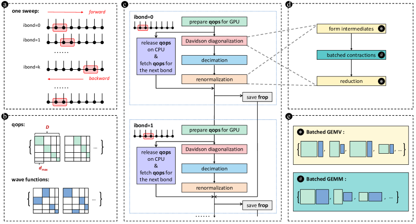
Figure 1: Flowchart of the two-dot sweep algorithm implemented in this work. Initially (ibond=0), all the necessary operators qops, see Eq. (19), which are stored in a block-sparse manner, are loaded from disk to CPU memory and then copied to GPU. Alternatively, if NVIDIA GPUDirect Storage (GDS) is supported, then qops can be directly loaded to GPU. Once the copy is finished, the CPU memory space is reused to prefetch qops for the next bond asynchronously in order to reduce IO time. In the Davidson diagonalization and renormalization steps, batched GEMV and GEMM are invoked on GPUs to form intermediates, perform contractions, and finally reduce to target results. After these two steps, the newly obtained renormalized operators are copied back to CPU, and then saved to disk asynchronously. The next cycle will start with copying qops from CPU to GPU (ibond=1). The iteration will go over the entire MPS chain and back to the initial bond, where a single DMRG sweep is finished.

2.3 Implementation details

This distributed multi-GPU ab initio DMRG algorithm is implemented in our in-house program Focus^{76, 77} written in C++ and CUDA. Here we provide a more detailed description of the implementation of batched contractions as well as other optimizations. The flowchart of the two-dot sweep algorithm implemented in this work is shown in Fig. 1. The detailed explanations are as follows. We refer the coordinate pair $(k,k+1)$ in the MPS chain (3) as a bond. A sweep consists of a sequence of bonds to be iterated, where at each bond either $A[k]$ or $A[k+1]$ will be updated depending on the sweep direction is forward or backward (see Fig. 1a). All the necessary normal and complementary operators^{78, 3, 6} for forming $\hat{O}^{L}$, $\hat{O}^{R}$, $\hat{O}^{C_{1}}$, and $\hat{O}^{C_{2}}$ in Eq. (5) at a given bond are named qops, which include

$$\{\hat{a}_{p}^{X\dagger},\hat{A}^{X}_{pq},\hat{B}^{X}_{ps},\hat{P}^{X}_{pq},\hat{Q}^{X}_{ps},\hat{S}^{X}_{p},\hat{H}^{X}\},\quad X\in\{L,R,C_{1},C_{2}\},$$ (19)

where

$$\hat{A}^{X}_{pq} = \hat{a}_{p}^{X\dagger}\hat{a}_{q}^{X\dagger},$$ (20)

$$\hat{B}^{X}_{ps} = \hat{a}_{p}^{X\dagger}\hat{a}^{X}_{s},$$ (21)

$$\hat{P}^{X}_{pq} = \sum_{s<r}\langle pq\|sr\rangle\hat{a}_{r}^{X}\hat{a}_{s}^{X},$$ (22)

$$\hat{Q}^{X}_{ps} = \sum_{qr}\langle pq\|sr\rangle\hat{a}_{q}^{X\dagger}\hat{a}_{r}^{X},$$ (23)

$$\hat{S}_{p} = \sum_{q}\frac{1}{2}h_{pq}\hat{a}_{q}^{X}+\sum_{q,s<r}\langle pq\|sr\rangle\hat{a}_{q}^{X\dagger}\hat{a}_{r}^{X}\hat{a}_{s}^{X}.$$ (24)

These operators are stored in a block-sparse manner (see Fig. 1b) using Abelian symmetries. At the initial bond, we first load qops from disk to CPU and then copy them from CPU to GPU (see Fig. 1c). Note that if NVIDIA GPUDirect Storage (GDS) is supported, qops can be directly loaded to GPU. In our implementation, we assume that both the CPU and GPU memories are large enough to hold the qops at a given bond, otherwise more nodes are needed. This will eventually become the bottleneck for extremely large-scale calculations, because the memory requirement for one process scales as $O(K^{2}D^{2}/n_{p}+KD^{2})$, where $O(KD^{2})$ comes from the storage for $\hat{a}_{p}$ and $\hat{S}_{p}$, which are duplicated in each process⁶ and will eventually become the bottleneck. Therefore, further optimizations are necessary to overcome this limitation in future. Once the copy is finished, we release the qops for the current bond on CPU, and use the memory space to prefetch qops for the next bond asynchronously. In this way, loading qops from disk to CPU memory, which will become time consuming for large-scale calculations, can be hided by the the Davidson diagonalization and renormalization steps. Similarly, after the renormalized operators are formed on GPU, they are copied back to CPU memory and then stored on disk asynchronously, which further hides the cost for IO by overlapping the saving process with the iteration for the next bond.

In both the Davidson and renormalization steps, batched GEMM of form Eq. (14) is the most computationally intensive part. In the DMRG++ code⁶⁶ for model Hamiltonians, it is handled with the MAGMA library⁷¹ (magmablas_dgemm_vbatched). In our test, we found the performance of such implementation for ab initio DMRG typically gives 5-6 TFLOPS on NVIDIA A100 GPU, which is about half of the peak performance for double precision using CUDA cores (9.7 TFLOPS). A more severe problem is that Tensor Cores are not supported yet by magmablas_dgemm_vbatched. To achieve better performance, a key observation is that different from the case for model Hamiltonians, for ab initio Hamiltonians (5) there are many operators in Eqs. (7) and (8) of the same kind (e.g. $\hat{a}_{p}^{X\dagger}$ for different $p$, $\hat{A}_{pq}^{X}$ for different $p<q$, etc.). This implies that GEMM encountered in Eq. (14) can be classified into groups by a simple sort, where within each group the dimensions are the same. To illustrate this fact, Figure 2 displays the distribution of groups for the batched GEMM in Eq. (11) appeared in the calculations of the P-cluster model with different bond dimensions $D$ and different number of processes $n_{p}$. In Table 1, we show the statistical analysis for the obtained results in Fig. 2. It is seen that the grouping strategy is very effective, in particular, for small $n_{p}$. We will refer the number of GEMMs of the same sizes as the batchCount as used in cuBLAS (cublasDgemmBatched). As shown in Table 1, for $n_{p}=4$ with $D=1000$ and $D=2000$, the averaged batchCount $N_{1}/N_{2}$ are greater than 100. This allows to effectively use the highly optimized kernel in cuBLAS (cublasDgemmBatched), which currently only supports batched GEMM for matrices with the same size and can use Tensor Cores for acceleration. When $n_{p}$ is increased to 16, the averaged batchCount $N_{1}/N_{2}$ becomes smaller, because the operators of the same type are eventually distributed to different processors as $n_{p}$ increases. This can lower the performance for small $D$. To take into account this, our final solution is to combine the use of batched GEMM with CUDA streams. For large $D$, the averaged cost for batched GEMM $C/N_{2}$ will become large enough to achieve good performance even with a small averaged batchCount $N_{1}/N_{2}$, since the size of the involved matrices will be increasingly large. Compared with using MAGMA, this combined approach leads to a much better performance (see Sec. 3).

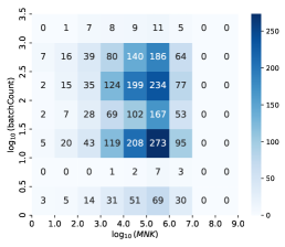
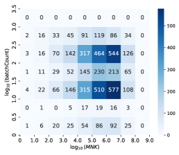
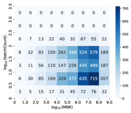
(a) $D=1000$ and $n_{p}=4$	(c) $D=2000$ and $n_{p}=4$	(e) $D=5000$ and $n_{p}=16$
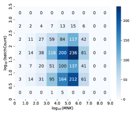
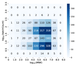
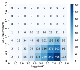
(b) $D=1000$ and $n_{p}=16$	(d) $D=2000$ and $n_{p}=16$	(f) $D=5000$ and $n_{p}=128$

Figure 2: Distribution of groups for the batched GEMM in Eq. (11) appeared in the DMRG calculations of the P-cluster model (ibond=34) with different bond dimensions $D$ and number of processes $n_{p}$. The data measured at rank 0 are displayed. The $x$ axis represents the cost of a single GEMM $C_{mn}=\sum_{k=1}^{K}A_{mk}B_{kn}$ ($m=1,\cdots,M$ and $n=1,\cdots,N$), while the $y$ axis represents the number of GEMMs of the same sizes ($M$, $N$, and $K$), which is referred as batchCount. The number shown in the graph represents the number of batched GEMM, that is, the number of function calls of the cuBLAS batched GEMM kernel, within the intervals.

Table 1: Statistical analysis for the distributions in Fig. 2. $n_{p}$: number of processors; $N_{1}$: total number of GEMM; $N_{2}$: total number of batched GEMM; $N_{1}/N_{2}$: averaged batchCount; $C$: total cost for GEMM (or equivalently batched GEMM) given by $\sum_{i=1}^{N_{1}}2M_{i}N_{i}K_{i}$; $C/N_{2}$: averaged cost for batched GEMM.

$D$	$n_{p}$	$N_{1}$	$N_{2}$	$N_{1}/N_{2}$	$C/10^{9}$	$C/N_{2}/10^{6}$
1000	4	508073	2666	190.6	386.1	144.8
1000	16	128196	2023	63.4	97.7	48.3
2000	4	625165	4972	125.7	2917.4	586.8
2000	16	157684	3092	51.0	736.3	238.1
5000	16	198853	6960	28.6	10323.0	1483.2
5000	128	27256	3293	8.3	1408.0	427.6

In this work, the program was tested on two different hardware platforms shown in Table 2. In the Davidson diagonalization, the formation and diagonalization of the Hamiltonian in a subspace, the computation of residuals and preconditioning, and the Gram-Schmidt orthonormalization are performed on CPU only at rank 0, while the formation of $\sigma$-vector in Eq. (13) is performed on distributed GPUs. We use the NVIDIA Collective Communication Library (NCCL)⁷⁹ to accelerate multi-GPU and multi-node communications for broadcasting trial vectors and the reduction of $\sigma$-vector in the Davidson step, as well as the reduction of complementary operators ($\hat{S}_{p}$ and $\hat{H}$) in the renormalization step.

Besides, we find the CPU part of the Davidson diagonalization on platform 1 with ARM processors using 32 threads is much slower than that on platform 2 with Intel processor using 8 threads, since some basic functions including dcopy, dnrm2, dgemm are slower using OpenBLAS than using MKL. To get a comparable performance, we reoptimize these functions for ARM processors. OpenMP is used for optimizing dcopy, while SIMD instruction and multi-threading techniques are used for optimizing dnrm2. For GEMM used in the Davidson step, we note that the special shape of matrices ($K\gg M,N$) necessitates the adoption of thread-level parallelism for all $M$/$N$/$K$ dimensions, while OpenBLAS’s inherent support for parallelism is only for the $M$ and $N$ dimensions. Besides, we have introduced a suite of assembly-level optimizations, comprising SIMD vectorization, loop unrolling, and prefetching. These optimizations, when applied within a 32-thread configuration, yield substantial performance enhancements, resulting in impressive speedup factors ranging from 10 to 15 compared with OpenBLAS in the calculations of the P-cluster with $D=8000$.

Table 2: Hardware platforms and software versions used in this work. The reported timing data were mostly obtained on platform 1, except for the blue lines in Fig. 4. The results in Table 5 requiring large CPU and GPU memory were obtained on platform 2.

	platform 1 (ARM)	platform 2 (Intel)
CPU	Huawei Kunpeng 920	Intel Xeon Gold 8358
no. of CPUs per node	2	2
CPU clockspeed	3.0 GHz	2.6 GHz
total no. of cores	128	64
CPU memory per node	250GB	1.5TB
GPU	NVIDIA A100 40GB PCIe	NVIDIA A100 80GB SXM
no. of GPUs per node	4	8
performance (FP64)	9.7 TFLOPS	9.7 TFLOPS
performance (FP64 Tensor Core)	19.5 TFLOPS	19.5 TFLOPS
GPU bandwidth	1555 GB/s	2039 GB/s
CUDA version	11.4	11.6
MPI version	OpenMPI 4.1.2	OpenMPI 4.1.5
NCCL version	2.16.5	2.17.1
MAGMA version	2.7.1	2.7.1
BLAS/LAPACK	OpenBLAS 0.3.23a	Intel MKL 2022
a Some BLAS functions (dcopy, dnrm2, and dgemm) are reoptimized for the ARM platform.

3 Results

We benchmark the performance of the above algorithm by applying it to the ground-state problem of an active space model (114 electrons in 73 active orbitals) defined in Ref. ³⁹ for the resting state of the P-cluster (see the inset of Fig. 6), where the integrals and orbital orderings are available online⁸⁰. Due to the limitation of computational resources, we performed timing analysis using platform 1 (ARM processors) with up to 32 nodes with 128 GPUs (NVIDIA A100 40GB) and $D\leq 8000$. In the last part of this section, a large-scale calculation using platform 2 (Intel processors), which has larger CPU and GPU memories per node, was reported using all the 6 nodes available with 48 GPUs (NVIDIA A100 80GB) in total and $D$ up to 14000.

Figure 3 shows the wall time for performing a single sweep and that for performing Eq. (7) in the Davidson step (referred as Hx for simplicity in the later context) of a single sweep, denoted by $T_{\mathrm{sweep}}$ and $T_{\mathrm{Hx}}$, respectively, as a function of the bond dimension $D$ or the number of GPUs $n_{\mathrm{GPU}}$. We find that both $T_{\mathrm{sweep}}$ and $T_{\mathrm{Hx}}$ scale roughly quadratically for large $D$, which is lower than the formal scaling $O(D^{3})$, while below $D=2500$ the scaling is lower than quadratic. These behaviors are attributed to the use of symmetries and GPUs. In Table 3, we list the maximal dimension of symmetry sectors $d_{\max}$ at a given bond dimension $D$ measured in the middle of the MPS chain. We find $d_{\max}$ and $D$ obey a simple linear relation for this system

$$d_{\max}(D)=0.128D+51.8.$$ (25)

Therefore, compared with the case without symmetry ($d_{\max}=D$), using Abelian symmetry leads to a 7.8 fold reduction of $d_{\max}$. This results in a very high block-sparsity in the operators and wavefunctions. Thus, the lowering from cubic to quadratic scaling is mainly due to the use of symmetry. Ref. ⁸¹ reported a similar scaling with respect to $D$, $O(D^{2.40})$ and $O(D^{2.18})$ for non-spin-adapted and spin-adapted DMRG, respectively, using 24 CPU cores for iron sulfur dimer. However, the gradual transition to quadratic scaling is not observed for small $D$. We attribute such transition to the use of GPU, because below certain $d_{\max}$ the workload is not enough to fill the GPU.

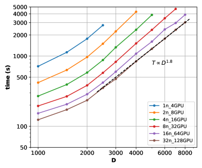
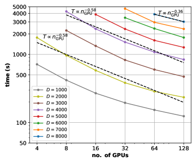
(a) Wall time for performing a single sweep $T_{\mathrm{sweep}}$ as a function of $D$ or $n_{\mathrm{GPU}}$.
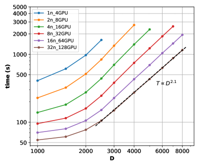
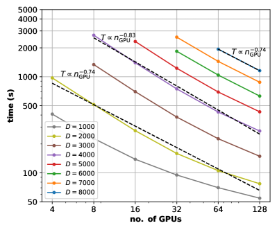
(b) Wall time for performing Eq. (7) in the Davidson step $T_{\mathrm{Hx}}$ as a function of $D$ or $n_{\mathrm{GPU}}$.

Figure 3: Wall time of performing a single sweep $T_{\mathrm{sweep}}$ and that for performing Eq. (7) in the Davidson step of a single sweep $T_{\mathrm{Hx}}$ as a function of the bond dimension $D$ or the number of GPUs $n_{\mathrm{GPU}}$ obtained on platform 1.

Table 3: Speedup for $T_{\mathrm{sweep}}$ and $T_{\mathrm{Hx}}$ (in parenthesis) for different bond dimensions $D$ using different number of nodes on platform 1, where each node has 4 GPUs. The column $d_{\max}$ lists the maximal dimension of symmetry sectors at a given bond dimension $D$ measured in the middle of the MPS chain (ibond=34). The last column shows the computed parallel efficiency. The symbol ’-’ indicates that the computation with a given $D$ cannot be done due to memory limitations, such that the parallel efficiency in the last column is calculated for the speedup with 32 nodes with respect to different references, where the number ’1’ indicates the reference for computing the speedup for a given $D$.

$D$	$d_{\max}$	1n	2n	4n	8n	16n	32n	efficiency
1000	167	1	1.7 (1.8)	2.6 (2.9)	3.6 (4.3)	4.5 (5.9)	5.6 (7.5)	0.17 (0.24)
2000	311	1	1.8 (1.9)	3.0 (3.5)	4.6 (6.1)	6.2 (9.2)	7.5 (12.6)	0.23 (0.40)
3000	442	-	1	1.7 (1.9)	2.6 (3.6)	3.6 (6.0)	4.5 (9.0)	0.28 (0.56)
4000	571	-	1	1.8 (1.9)	2.8 (3.6)	4.0 (6.3)	5.1 (9.9)	0.32 (0.62)
5000	697	-	-	1	1.6 (1.9)	2.4 (3.4)	3.0 (5.4)	0.38 (0.67)
6000	820	-	-	-	1	1.4 (1.8)	2.0 (2.9)	0.49 (0.73)
7000	944	-	-	-	1	1.6 (1.8)	2.0 (2.9)	0.50 (0.74)
8000	1071	-	-	-	-	1	1.3 (1.7)	0.64 (0.84)

The strong scaling is also illustrated in Fig. 3, and the detailed results for speedup is shown in Table 3 for different bond dimensions with different number of nodes. Overall, it is seen that $T_{\mathrm{Hx}}$ scales much better than $T_{\mathrm{sweep}}$. For instance, $T_{\mathrm{sweep}}$ for $D=8000$ with 128 GPUs becomes $2^{-0.36}=78\%$ of that with 64 GPUs, whereas $T_{\mathrm{Hx}}$ for $D=8000$ with 128 GPUs is about $2^{-0.74}=60\%$ of that with 64 GPUs. The decreases of speedup for the entire sweep is analyzed latter. Now we focus on the analysis of the speedup only for $T_{\mathrm{Hx}}$, where a decomposition of the speedup for different parts of Hx is shown in Table 4. There are several factors that affect the total speedup for Hx. Firstly, for small bond dimensions such as $D=1000$ or $D=2000$, the speedup for Hx is not ideal with 32 nodes, because the workload is not large enough. This is reflected in the Fig. 3(b), where the curves start to deviate from being linear as $n_{\mathrm{GPU}}$ is greater than 32 for $D=1000$ and $D=2000$. Generally, we can observe that the parallel efficiency increases as the bond dimension increases. Secondly, the calculation at the middle of the MPS chain scales better than that close to the boundary of the MPS chain, since the bond dimension close to the boundary is actually smaller than $D$. This can be seen from the comparison in Table 4 between the speedups for a single sweep and the corresponding results for the middle of the sweep. Thirdly, the total speedup for Hx can be slightly smaller than those for the three computational steps as shown for $D=8000$, because in addition to computations, $T_{\mathrm{Hx}}$ also includes the time for communication between different nodes for broadcasting the trial vector and reducing the $\sigma$-vector as well as the time for copying the trial vector from CPU to GPU and the $\sigma$-vector from GPU back to CPU. These parts take less than 10% of $T_{\mathrm{Hx}}$ in our tests for $D\geq 5000$ with 32 nodes.

Table 4: Speedup for different parts of $T_{\mathrm{Hx}}$ in a single sweep obtained using 32 nodes for $D$=2000, 5000, and 8000, with respect to those obtained using 1, 4, and 16 nodes, respectively. The three steps (intermediates, GEMM, reduction) refer to different computational steps in performing Eqs. (9)-(13), see also Fig. 1d. Values in parenthesis are the corresponding speedups for the middle of the sweep (ibond=34).

$D$	reference	intermediates	GEMM	reduction	Hx
2000	1n	23.4 (27.1)	12.2 (20.9)	14.1 (21.0)	12.6 (19.7)
5000	4n	6.4 (7.4)	5.9 (7.1)	5.1 (6.5)	5.4 (6.6)
8000	16n	1.8 (1.9)	1.8 (1.9)	1.7 (1.9)	1.7 (1.8)

In Fig. 4, we show the average performances for the eight batches of GEMM in Eqs. (9)-(12) in the Davidson step and those in Eqs. (15)-(17) in the renormalization step as a function of $D$ measured at the bond in the middle of the MPS chain. It is clear that in both cases the performances increase as $D$ increases. The performances above $D=3000$ exceed the theoretical peak performance for double-precision floating-point format (FP64) using CUDA Cores. Therefore, using Tensor Cores leads to a significant increase in performance and hence reduces the computational time dramatically. The peak performance obtained on NVIDIA A100 PCIe 40 GB is about 13 TFLOPS, which is 67% of the peak performance for FP64 with Tensor Cores, while that obtained on NVIDIA A100 SMX 80 GB is about 15 TFLOPS, which is 10% higher. To better understand the performance, we also plot the measured performances of cublasDgemmBatched for a single batched GEMM with $M=N=K=d_{\max}(D)$, where $d_{\max}(D)$ is given in Eq. (25), and the batchCount is determined by fixing the total memory of all matrices ($\mathrm{batchCount}\times 3d^{2}_{\max}(D)$) to be 10 GB. This can roughly be considered as an upper bond for our implementation. Because the actual GPU memory available may be smaller for large $D$, and the sizes of most matrices in the batched GEMM are smaller than $d_{\max}$. It is seen that the performance of our combined strategy using batched GEMM and CUDA streams is about 85% of this model for large $D$. Finally, we observe that the performances with less processes are higher in particular for $D$ less than 2000. This is because as shown in Fig. 2, the batchCount is smaller for larger $n_{\mathrm{GPU}}$. This indicates a room for further improving the performance for larger $n_{\mathrm{GPU}}$ in future, by combining different batched GEMM together in the case of small matrices.

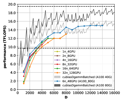
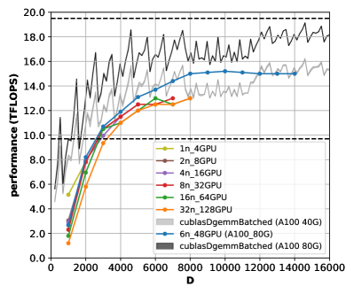
Figure 4: Average performances for the eight batches of GEMM in Eqs. (9)-(12) in the Davidson step and those in Eqs. (15)-(17) in the renormalization step as a function of $D$. The data are measured at rank 0 in the DMRG calculation for the bond in the middle of the MPS chain (ibond=34). The black dashed lines are the theoretical performances for double precision using CUDA Cores (9.7 TFLOPS) and Tensor Cores (19.5 TFLOPS), respectively. The black and grey lines are the measured performances of cublasDgemmBatched for a single batched GEMM with $M=N=K=d_{\max}(D)$, where $d_{\max}(D)$ is given in Eq. (25), and the batchCount is determined by fixing the total memory of all matrices ($\mathrm{batchCount}\times 3d^{2}_{\max}(D)$) to be 10 GB. Except for the blue and black lines, which were obtained on platform 2 using NVIDIA A100 SXM 80 GB, all the data were obtained on platform 1 using NVIDIA A100 PCIe 40 GB.

As mentioned before in Table 3, the speedup for $T_{\mathrm{sweep}}$ is lower than that for $T_{\mathrm{Hx}}$. Figure 5 shows the decomposition of $T_{\mathrm{sweep}}$ for $D=3000$, $D=5000$, and $D=7000$ into different parts. The part $T_{\mathrm{Hx}}$ is always the dominant part of the DMRG calculations, which is known in previous DMRG studies^{10, 62}. In comparison, the renormalization part is quite small. The reduction of $T_{\mathrm{Hx}}$, $T_{\mathrm{renorm}}$, and $T_{\mathrm{IO}}$ by using more nodes is reasonably good. Thus, our goal to accelerate the most expensive part in DMRG using multi-GPUs has been achieved. In the current implementation, the decimation step is simply done on CPU, which can also be carried out on GPU using cuSOLVER. We note that the rest part starts to become a larger portion as the number of nodes increases, and hence it needs to be optimized in future in order to achieve better scalability for $T_{\mathrm{sweep}}$. One major contribution to this part is the serial part in the Davidson diagonalization, which is executed only on CPU at rank 0. If a better iterative eigensolver is implemented, we expect that the wall time for this part can be reduced.

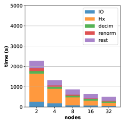
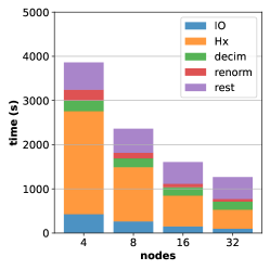
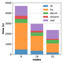
(a) $D=3000$	(b) $D=5000$	(c) $D=7000$

Figure 5: Decomposition of $T_{\mathrm{sweep}}$ for $D=3000$, $D=5000$, and $D=7000$ obtained on platform 1 into IO, Hx, decimation, renormalization and the rest part, which includes the serial part of the Davidson diagonalization, the construction of the diagonal part of Hamiltonian, other communication and synchronization, etc.

Finally, as an example to illustrate the capability of the present algorithm, we performed a large-scale DMRG calculation for the P-cluster model using platform 2 with $D$ up to 14000, and compared the obtained energies $E$ and discarded weights $w$ with those previously obtained^{39, 41} using spin-adapted DMRG on CPUs in Table 5. The largest $D$ achieved in the present work is nearly three times larger than that reported in previous works for the same system using only CPUs with MPI/OpenMP parallelization. Calculations with larger $D$ are possible provided more GPUs are available for meeting the memory requirement. The energy differences between the present and the previous works for the same $D$ are mainly due to two factors. First, the initial guesses for MPS are different. While the initial guess in previous studies was obtained from spin-projected MPS⁵⁶ with a small bond dimension, the initial guess in the present work is generated from the conversion of a selected configuration interaction (SCI) wavefunction following Ref. ⁷⁶. Second, the present implementation only using Abelian symmetries is non-spin-adapted. However, we found that the DMRG energy with the same $D$ obtained in the present work is lower than the corresponding result obtained in previous works. This is usually not the case for calculations with and without spin-adaptation, as spin-adaptation can lead to much lower energy for spin-coupled systems²³. Therefore, the energy difference is mainly due to the different initialization strategies. This is also reflected in the discarded weights, where the present results are smaller than the previous results^{39, 41} for the same $D$.

Table 5: Comparison of DMRG energies ($E$ in Hartree) and discarded weights ($w$) obtained for the P-cluster CAS(114e,73o) model. Previous results taken from Refs. ³⁹ and ⁴¹ were obtained with spin-adapted DMRG, while the present results were obtained without spin-adaptation. The last line shows the extrapolated energy $E_{w=0}$ obtained via a linear extrapolation $E(w)=Aw+E_{w=0}$ shown in Fig. 6.

Li et al. (Ref. 39)				Lee et al. (Ref. 41)				this work
$D$	$w$	$E$		$D$	$w$	$E$		$D$	$w$	$E$
3000	2.30$\times 10^{-4}$	-17492.213966		1000	4.17$\times 10^{-4}$	-17492.190311		2000	1.24$\times 10^{-4}$	-17492.215587
3500	2.00$\times 10^{-4}$	-17492.216321		1500	3.40$\times 10^{-4}$	-17492.200594		3000	9.87$\times 10^{-5}$	-17492.220314
4000	1.60$\times 10^{-4}$	-17492.218127		2000	2.89$\times 10^{-4}$	-17492.206725		4000	8.35$\times 10^{-5}$	-17492.222921
				2500	2.51$\times 10^{-4}$	-17492.210894		5000	7.31$\times 10^{-5}$	-17492.224618
				3000	2.23$\times 10^{-4}$	-17492.213953		6000	6.58$\times 10^{-5}$	-17492.225828
				3500	2.00$\times 10^{-4}$	-17492.216294		7000	5.98$\times 10^{-5}$	-17492.226734
				4000	1.82$\times 10^{-4}$	-17492.218146		8000	5.52$\times 10^{-5}$	-17492.227448
				4500	1.63$\times 10^{-4}$	-17492.219644		9000	5.15$\times 10^{-5}$	-17492.228023
				5000	1.36$\times 10^{-4}$	-17492.220847		10000	4.83$\times 10^{-5}$	-17492.228500
								11000	4.53$\times 10^{-5}$	-17492.228900
								12000	4.28$\times 10^{-5}$	-17492.229245
								13000	4.04$\times 10^{-5}$	-17492.229539
								14000	3.83$\times 10^{-5}$	-17492.229797
extrapolation		-17492.227676				-17492.237907				-17492.236408

In the last line of Table 5, we report the extrapolated energies using a linear extrapolation with respect to the discarded weights, see Fig. 6. It is seen that while the earliest extrapolated energy³⁹ with only a few data points seems to overestimate the ground-state energy, the extrapolated results obtained with the data from Ref. ⁴¹ and the present work agree within 1 mH. Our best variational energy obtained with $D=14000$ differs from the extrapolated energy by 6.6 mH, while the difference for the previous results⁴¹ is 17.1 mH. Thus, a reduction of the error by a factor of almost three is achieved using the new hybrid CPU-GPU implementation, and the error per metal is within 1 mH compared with the extrapolated energies. It deserves to point out that as shown in the last column of Table 5, the energy converges very slowly as $D$ increases, which is an indication of the complex entanglement structure for the P-cluster problem. We expect that using SU(2) symmetry in future can accelerate the convergence.

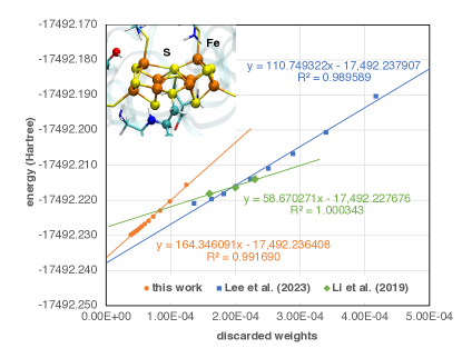
Figure 6: Comparison of linear extrapolation of DMRG energies $E$ with respect to discarded weights $w$ obtained in the present and previous studies^{39, 41} for the P-cluster CAS(114e,73o) model.

4 Conclusion

In this work, we presented a distributed multi-GPU ab initio DMRG algorithm suitable for modern heterogeneous HPC infrastructures. This is achieved by combining the operator parallelism¹⁰ using MPI and batched matrix-vector and matrix-matrix multiplications using GPUs. In particular, we show that the algorithm enables the use of Tensor Cores for accelerating GEMM, which is the most computationally expensive part in DMRG. With this new development, we can reach an unprecedented accuracy (1 mH per metal) for the ground-state energy of a CAS(114e,73o) model^{39, 80} of the P-cluster with a bond dimension $D=14000$.

The present algorithm can be readily combined with other techniques to further improve the performance of ab initio DMRG, such as SU(2) symmetry, real-space parallelization⁶⁰, and mixed-precision schemes⁸². We are also interested in applying the present algorithm to fully relativistic DMRG^{32, 83, 84, 77}, where the symmetry is lower and hence the symmetry blocks are much larger and complex algebra is required. We expect in such case the GPU acceleration will be even more beneficial.

We acknowledge Dingshun Lv, Qiaorui Chen, and Zhen Guo for helpful discussions on batched matrix-matrix multiplications on GPU, and Bingbing Suo for useful comments on the manuscript. This work was supported by the National Natural Science Foundation of China (Grants No. 21973003) and the Fundamental Research Funds for the Central Universities. We acknowledge the computing resource and technical support provided by Tan Kah Kee Supercomputing Center (IKKEM).

References

- White 1992 White, S. R. Density matrix formulation for quantum renormalization groups. Phys. Rev. Lett. 1992, 69, 2863
- White 1993 White, S. R. Density-matrix algorithms for quantum renormalization groups. Phys. Rev. B 1993, 48, 10345
- White and Martin 1999 White, S. R.; Martin, R. L. Ab initio quantum chemistry using the density matrix renormalization group. J. Chem. Phys. 1999, 110, 4127–4130
- Daul et al. 2000 Daul, S.; Ciofini, I.; Daul, C.; White, S. R. Full-CI quantum chemistry using the density matrix renormalization group. Int. J. Quantum Chem. 2000, 79, 331–342
- Mitrushenkov et al. 2001 Mitrushenkov, A. O.; Fano, G.; Ortolani, F.; Linguerri, R.; Palmieri, P. Quantum chemistry using the density matrix renormalization group. J. Chem. Phys. 2001, 115, 6815–6821
- Chan and Head-Gordon 2002 Chan, G. K.-L.; Head-Gordon, M. Highly correlated calculations with a polynomial cost algorithm: A study of the density matrix renormalization group. J. Chem. Phys. 2002, 116, 4462–4476
- Chan and Head-Gordon 2003 Chan, G. K.-L.; Head-Gordon, M. Exact solution (within a triple-zeta, double polarization basis set) of the electronic Schrödinger equation for water. J. Chem. Phys. 2003, 118, 8551–8554
- Legeza et al. 2003 Legeza, Ö.; Röder, J.; Hess, B. Controlling the accuracy of the density-matrix renormalization-group method: The dynamical block state selection approach. Phys. Rev. B 2003, 67, 125114
- Legeza and Sólyom 2003 Legeza, Ö.; Sólyom, J. Optimizing the density-matrix renormalization group method using quantum information entropy. Phys. Rev. B 2003, 68, 195116
- Chan 2004 Chan, G. K.-L. An algorithm for large scale density matrix renormalization group calculations. J. Chem. Phys. 2004, 120, 3172–3178
- Mitrushenkov et al. 2003 Mitrushenkov, A.; Linguerri, R.; Palmieri, P.; Fano, G. Quantum chemistry using the density matrix renormalization group II. J. Chem. Phys. 2003, 119, 4148–4158
- Chan et al. 2004 Chan, G. K.-L.; Kállay, M.; Gauss, J. State-of-the-art density matrix renormalization group and coupled cluster theory studies of the nitrogen binding curve. J. Chem. Phys. 2004, 121, 6110–6116
- Chan and Van Voorhis 2005 Chan, G. K.-L.; Van Voorhis, T. Density-matrix renormalization-group algorithms with nonorthogonal orbitals and non-Hermitian operators, and applications to polyenes. J. Chem. Phys. 2005, 122, 204101
- Moritz and Reiher 2006 Moritz, G.; Reiher, M. Construction of environment states in quantum-chemical density-matrix renormalization group calculations. J. Chem. Phys. 2006, 124, 034103
- Hachmann et al. 2006 Hachmann, J.; Cardoen, W.; Chan, G. K.-L. Multireference correlation in long molecules with the quadratic scaling density matrix renormalization group. J. Chem. Phys. 2006, 125, 144101
- Marti et al. 2008 Marti, K. H.; Ondík, I. M.; Moritz, G.; Reiher, M. Density matrix renormalization group calculations on relative energies of transition metal complexes and clusters. J. Chem. Phys. 2008, 128, 014104
- Ghosh et al. 2008 Ghosh, D.; Hachmann, J.; Yanai, T.; Chan, G. K.-L. Orbital optimization in the density matrix renormalization group, with applications to polyenes and -carotene. J. Chem. Phys. 2008, 128, 144117
- Chan 2008 Chan, G. K.-L. Density matrix renormalisation group Lagrangians. Phys. Chem. Chem. Phys. 2008, 10, 3454–3459
- Zgid and Nooijen 2008 Zgid, D.; Nooijen, M. Obtaining the two-body density matrix in the density matrix renormalization group method. J. Chem. Phys. 2008, 128, 144115
- Luo et al. 2010 Luo, H.-G.; Qin, M.-P.; Xiang, T. Optimizing Hartree-Fock orbitals by the density-matrix renormalization group. Phys. Rev. B 2010, 81, 235129
- Marti and Reiher 2011 Marti, K. H.; Reiher, M. New electron correlation theories for transition metal chemistry. Phys. Chem. Chem. Phys. 2011, 13, 6750–6759
- Kurashige and Yanai 2011 Kurashige, Y.; Yanai, T. Second-order perturbation theory with a density matrix renormalization group self-consistent field reference function: Theory and application to the study of chromium dimer. J. Chem. Phys. 2011, 135, 094104
- Sharma and Chan 2012 Sharma, S.; Chan, G. K.-L. Spin-adapted density matrix renormalization group algorithms for quantum chemistry. J. Chem. Phys. 2012, 136, 124121
- Chan 2012 Chan, G. K. Low entanglement wavefunctions. Wiley Interdiscip. Rev. Comput. Mol. Sci. 2012, 2, 907–920
- Wouters et al. 2012 Wouters, S.; Limacher, P. A.; Van Neck, D.; Ayers, P. W. Longitudinal static optical properties of hydrogen chains: Finite field extrapolations of matrix product state calculations. J. Chem. Phys. 2012, 136, 134110
- Mizukami et al. 2012 Mizukami, W.; Kurashige, Y.; Yanai, T. More electrons make a difference: Emergence of many radicals on graphene nanoribbons studied by ab initio DMRG theory. J. Chem. Theory Comput. 2012, 9, 401–407
- Kurashige et al. 2013 Kurashige, Y.; Chan, G. K.-L.; Yanai, T. Entangled quantum electronic wavefunctions of the Mn4CaO5 cluster in photosystem II. Nat. Chem. 2013, 5, 660–666
- Sharma et al. 2014 Sharma, S.; Sivalingam, K.; Neese, F.; Chan, G. K.-L. Low-energy spectrum of iron–sulfur clusters directly from many-particle quantum mechanics. Nat. Chem. 2014, 6, 927–933
- Wouters and Van Neck 2014 Wouters, S.; Van Neck, D. The density matrix renormalization group for ab initio quantum chemistry. Eur. Phys. J. D 2014, 68, 1–20
- Wouters et al. 2014 Wouters, S.; Poelmans, W.; Ayers, P. W.; Van Neck, D. CheMPS2: A free open-source spin-adapted implementation of the density matrix renormalization group for ab initio quantum chemistry. Comput. Phys. Commun. 2014, 185, 1501–1514
- Fertitta et al. 2014 Fertitta, E.; Paulus, B.; Barcza, G.; Legeza, Ö. Investigation of metal–insulator-like transition through the ab initio density matrix renormalization group approach. Phys. Rev. B 2014, 90, 245129
- Knecht et al. 2014 Knecht, S.; Legeza, Ö.; Reiher, M. Communication: Four-component density matrix renormalization group. J. Chem. Phys. 2014, 140, 041101
- Szalay et al. 2015 Szalay, S.; Pfeffer, M.; Murg, V.; Barcza, G.; Verstraete, F.; Schneider, R.; Legeza, Ö. Tensor product methods and entanglement optimization for ab initio quantum chemistry. Int. J. Quantum Chem. 2015, 115, 1342–1391
- Yanai et al. 2015 Yanai, T.; Kurashige, Y.; Mizukami, W.; Chalupskỳ, J.; Lan, T. N.; Saitow, M. Density matrix renormalization group for ab initio Calculations and associated dynamic correlation methods: A review of theory and applications. Int. J. Quantum Chem. 2015, 115, 283–299
- Olivares-Amaya et al. 2015 Olivares-Amaya, R.; Hu, W.; Nakatani, N.; Sharma, S.; Yang, J.; Chan, G. K.-L. The ab-initio density matrix renormalization group in practice. J. Chem. Phys. 2015, 142, 034102
- Baiardi and Reiher 2020 Baiardi, A.; Reiher, M. The density matrix renormalization group in chemistry and molecular physics: Recent developments and new challenges. J. Chem. Phys. 2020, 152
- Cheng et al. 2022 Cheng, Y.; Xie, Z.; Ma, H. Post-density matrix renormalization group methods for describing dynamic electron correlation with large active spaces. J. Phys. Chem. Lett. 2022, 13, 904–915
- Ma et al. 2022 Ma, H.; Schollwöck, U.; Shuai, Z. Density Matrix Renormalization Group (DMRG)-Based Approaches in Computational Chemistry; Elsevier, 2022
- Li et al. 2019 Li, Z.; Guo, S.; Sun, Q.; Chan, G. K.-L. Electronic landscape of the P-cluster of nitrogenase as revealed through many-electron quantum wavefunction simulations. Nat. Chem. 2019, 11, 1026–1033
- Li et al. 2019 Li, Z.; Li, J.; Dattani, N. S.; Umrigar, C.; Chan, G. K. The electronic complexity of the ground-state of the FeMo cofactor of nitrogenase as relevant to quantum simulations. J. Chem. Phys. 2019, 150
- Lee et al. 2023 Lee, S.; Lee, J.; Zhai, H.; Tong, Y.; Dalzell, A. M.; Kumar, A.; Helms, P.; Gray, J.; Cui, Z.-H.; Liu, W., et al. Evaluating the evidence for exponential quantum advantage in ground-state quantum chemistry. Nat. Commun. 2023, 14, 1952
- Eisert et al. 2010 Eisert, J.; Cramer, M.; Plenio, M. B. Colloquium: Area laws for the entanglement entropy. Rev. Mod. Phys. 2010, 82, 277
- 43 \urlwww.top500.org
- Ufimtsev and Martinez 2008 Ufimtsev, I. S.; Martinez, T. J. Graphical processing units for quantum chemistry. Comput. Sci. Eng. 2008, 10, 26–34
- Seritan et al. 2021 Seritan, S.; Bannwarth, C.; Fales, B. S.; Hohenstein, E. G.; Isborn, C. M.; Kokkila-Schumacher, S. I.; Li, X.; Liu, F.; Luehr, N.; Snyder Jr, J. W., et al. TeraChem: A graphical processing unit-accelerated electronic structure package for large-scale ab initio molecular dynamics. Wiley Interdiscip. Rev. Comput. Mol. Sci. 2021, 11, e1494
- Zahariev et al. 2023 Zahariev, F.; Xu, P.; Westheimer, B. M.; Webb, S.; Galvez Vallejo, J.; Tiwari, A.; Sundriyal, V.; Sosonkina, M.; Shen, J.; Schoendorff, G., et al. The General Atomic and Molecular Electronic Structure System (GAMESS): Novel Methods on Novel Architectures. J. Chem. Theory Comput. 2023,
- Kussmann and Ochsenfeld 2017 Kussmann, J.; Ochsenfeld, C. Hybrid CPU/GPU integral engine for strong-scaling ab initio methods. J. Chem. Theory Comput. 2017, 13, 3153–3159
- Hacene et al. 2012 Hacene, M.; Anciaux-Sedrakian, A.; Rozanska, X.; Klahr, D.; Guignon, T.; Fleurat-Lessard, P. Accelerating VASP electronic structure calculations using graphic processing units. J. Comput. Chem. 2012, 33, 2581–2589
- Hutchinson and Widom 2012 Hutchinson, M.; Widom, M. VASP on a GPU: Application to exact-exchange calculations of the stability of elemental boron. Comput. Phys. Commun. 2012, 183, 1422–1426
- Jia et al. 2013 Jia, W.; Cao, Z.; Wang, L.; Fu, J.; Chi, X.; Gao, W.; Wang, L.-W. The analysis of a plane wave pseudopotential density functional theory code on a GPU machine. Comput. Phys. Commun. 2013, 184, 9 – 18
- Jia et al. 2013 Jia, W.; Fu, J.; Cao, Z.; Wang, L.; Chi, X.; Gao, W.; Wang, L.-W. Fast plane wave density functional theory molecular dynamics calculations on multi-GPU machines. J. Comput. Phys. 2013, 251, 102 – 115
- Romero et al. 2018 Romero, J.; Phillips, E.; Ruetsch, G.; Fatica, M.; Spiga, F.; Giannozzi, P. A Performance Study of Quantum ESPRESSO’s PWscf Code on Multi-core and GPU Systems. High Performance Computing Systems. Performance Modeling, Benchmarking, and Simulation. Cham, 2018; pp 67–87
- Ben et al. 2020 Ben, M. D.; Yang, C.; Li, Z.; Jornada, F. H. d.; Louie, S. G.; Deslippe, J. Accelerating Large-Scale Excited-State GW Calculations on Leadership HPC Systems. SC20: International Conference for High Performance Computing, Networking, Storage and Analysis. 2020; pp 1–11
- Markidis et al. 2018 Markidis, S.; Chien, S. W. D.; Laure, E.; Peng, I. B.; Vetter, J. S. NVIDIA Tensor Core Programmability, Performance & Precision. 2018 IEEE International Parallel and Distributed Processing Symposium Workshops (IPDPSW). 2018; pp 522–531
- Kurashige and Yanai 2009 Kurashige, Y.; Yanai, T. High-performance ab initio density matrix renormalization group method: Applicability to large-scale multireference problems for metal compounds. J. Chem. Phys. 2009, 130, 234114
- Li and Chan 2017 Li, Z.; Chan, G. K.-L. Spin-projected matrix product states: Versatile tool for strongly correlated systems. J. Chem. Theory Comput. 2017, 13, 2681–2695
- Chan et al. 2016 Chan, G. K.; Keselman, A.; Nakatani, N.; Li, Z.; White, S. R. Matrix product operators, matrix product states, and ab initio density matrix renormalization group algorithms. J. Chem. Phys. 2016, 145
- Brabec et al. 2021 Brabec, J.; Brandejs, J.; Kowalski, K.; Xantheas, S.; Legeza, Ö.; Veis, L. Massively parallel quantum chemical density matrix renormalization group method. J. Comput. Chem. 2021, 42, 534–544
- Zhai and Chan 2021 Zhai, H.; Chan, G. K. Low communication high performance ab initio density matrix renormalization group algorithms. J. Chem. Phys. 2021, 154
- Stoudenmire and White 2013 Stoudenmire, E.; White, S. R. Real-space parallel density matrix renormalization group. Phys. Rev. B 2013, 87, 155137
- Menczer and Legeza 2023 Menczer, A.; Legeza, Ö. Massively Parallel Tensor Network State Algorithms on Hybrid CPU-GPU Based Architectures. arXiv preprint arXiv:2305.05581 2023,
- Menczer and Legeza 2023 Menczer, A.; Legeza, Ö. Boosting the effective performance of massively parallel tensor network state algorithms on hybrid CPU-GPU based architectures via non-Abelian symmetries. arXiv preprint arXiv:2309.16724 2023,
- Hager et al. 2004 Hager, G.; Jeckelmann, E.; Fehske, H.; Wellein, G. Parallelization strategies for density matrix renormalization group algorithms on shared-memory systems. J. Comput. Phys. 2004, 194, 795–808
- Levy et al. 2020 Levy, R.; Solomonik, E.; Clark, B. K. Distributed-memory DMRG via sparse and dense parallel tensor contractions. SC20: International Conference for High Performance Computing, Networking, Storage and Analysis. 2020; pp 1–14
- Nemes et al. 2014 Nemes, C.; Barcza, G.; Nagy, Z.; Legeza, Ö.; Szolgay, P. The density matrix renormalization group algorithm on kilo-processor architectures: Implementation and trade-offs. Comput. Phys. Commun. 2014, 185, 1570–1581
- Elwasif et al. 2018 Elwasif, W.; D’azevedo, E.; Chatterjee, A.; Alvarez, G.; Hernandez, O.; Sarkar, V. MiniApp for Density Matrix Renormalization Group Hamiltonian Application Kernel. 2018 IEEE International Conference on Cluster Computing (CLUSTER). 2018; pp 590–597
- Li et al. 2020 Li, W.; Ren, J.; Shuai, Z. Numerical assessment for accuracy and GPU acceleration of TD-DMRG time evolution schemes. J. Chem. Phys. 2020, 152
- Chen et al. 2020 Chen, F.-Z.; Cheng, C.; Luo, H.-G. Improved hybrid parallel strategy for density matrix renormalization group method. Chin. Phys. B 2020, 29, 070202
- Chen et al. 2021 Chen, F.-Z.; Cheng, C.; Luo, H.-G. Real-space parallel density matrix renormalization group with adaptive boundaries. Chin. Phys. B 2021, 30, 080202
- Ganahl et al. 2023 Ganahl, M.; Beall, J.; Hauru, M.; Lewis, A. G.; Wojno, T.; Yoo, J. H.; Zou, Y.; Vidal, G. Density matrix renormalization group with tensor processing units. PRX Quantum 2023, 4, 010317
- Abdelfattah et al. 2016 Abdelfattah, A.; Haidar, A.; Tomov, S.; Dongarra, J. Performance, design, and autotuning of batched GEMM for GPUs. High Performance Computing: 31st International Conference, ISC High Performance 2016, Frankfurt, Germany, June 19-23, 2016, Proceedings. 2016; pp 21–38
- Tian and Ma 2023 Tian, Y.; Ma, H. High-Performance Computing for Density Matrix Renormalization Group. Curr. Chin. Sci. 2023, 3, 178–186
- Schollwöck 2011 Schollwöck, U. The density-matrix renormalization group in the age of matrix product states. Ann. Phys. 2011, 326, 96–192
- Davidson 1975 Davidson, E. R. The iterative calculation of a few of the lowest eigenvalues and corresponding eigenvectors of large real-symmetric matrices. J. Comput. Phys 1975, 17, 87–94
- Walker and Dongarra 1996 Walker, D. W.; Dongarra, J. J. MPI: a standard message passing interface. Supercomputer 1996, 12, 56–68
- Li 2021 Li, Z. Expressibility of comb tensor network states (CTNS) for the P-cluster and the FeMo-cofactor of nitrogenase. Electron. struct. 2021, 3, 014001
- Li 2023 Li, Z. Time-reversal symmetry adaptation in relativistic density matrix renormalization group algorithm. J. Chem. Phys. 2023, 158
- Xiang 1996 Xiang, T. Density-matrix renormalization-group method in momentum space. Phys. Rev. B 1996, 53, R10445
- 79 https://developer.nvidia.com/nccl
- 80 https://github.com/zhendongli2008/Active-space-model-for-Pclusters
- Zhai et al. 2023 Zhai, H.; Larsson, H. R.; Lee, S.; Cui, Z.-H.; Zhu, T.; Sun, C.; Peng, L.; Peng, R.; Liao, K.; Tölle, J., et al. Block2: a comprehensive open source framework to develop and apply state-of-the-art DMRG algorithms in electronic structure and beyond. arXiv preprint arXiv:2310.03920 2023,
- Tian et al. 2022 Tian, Y.; Xie, Z.; Luo, Z.; Ma, H. Mixed-Precision Implementation of the Density Matrix Renormalization Group. J. Chem. Theory Comput. 2022, 18, 7260–7271
- Battaglia et al. 2018 Battaglia, S.; Keller, S.; Knecht, S. Efficient relativistic density-matrix renormalization group implementation in a matrix-product formulation. J. Chem. Theory Comput. 2018, 14, 2353–2369
- Zhai and Chan 2022 Zhai, H.; Chan, G. K. A comparison between the one-and two-step spin–orbit coupling approaches based on the ab initio density matrix renormalization group. J. Chem. Phys. 2022, 157