Steady-State Analysis and Online Learning for Queues with Hawkes Arrivals

Abstract

We investigate the long-run behavior of single-server queues with Hawkes arrivals and general service distributions and related optimization problems. In detail, utilizing novel coupling techniques, we establish finite moment bounds for the stationary distribution of the workload and busy period processes. In addition, we are able to show that, those queueing processes converge exponentially fast to their stationary distribution. Based on these theoretic results, we develop an efficient numerical algorithm to solv the optimal staffing problem for the Hawkes queues in a data-driven manner. Numerical results indicate a sharp difference in staffing for Hawkes queues, compared to the classic GI/GI/1 model, especially in the heavy-traffic regime.

Keywords: steady-state analysis; Hawkes processes; capacity sizing problem; online learning

1 Introduction

As one of the most fundamental queueing model, the single-server queue is used to describe service systems with scarce but reusable recourse. Recent empirical studies found that arrivals in many real queueing systems exhibit a clustering or self-exciting behavior; that is, an arrival may increase the possibility of new arrivals. In some cases, such clustering behavior is intrinsic to the underlying system. For example, in the stock market, it is a common practice to split a large order into small child orders to reduce transaction cost. As a consequence, one observed arriving order may be followed by a sequence of other child orders (Abergel and Jedidi, 2015). As a natural extension of the classic Poisson process, Hawkes process has been used to model arrivals with self-excitement such as order flow in stock market (Abergel and Jedidi, 2015), infected patients during pandemic (Bertozzi et al., 2020), and the internet traffic in social media (Zhao et al., 2015).

To understand the impact of self-excitement in the arrival process on the long-run performance of service systems, Koops et al. (2018) and Daw and Pender (2018) provided analytic solutions to steady-state moments on the number of people in system for different infinite-server systems with Hawkes arrivals. In particular, Daw and Pender (2018) study the systems with Markovian Hawkes arrivals and phase-type/deterministic service times, whereas Koops et al. (2018) study the cases with non-Markovian Hawkes arrivals and exponential service times. Because of the dependence between customer arrivals and sojourn times, it is difficult to obtain analytic results for finite-server queues with Hawkes arrivals, including the most fundamental single-server queue (see the dicussion on p.941 of Koops et al. (2018)). Instead, simulation algorithm was developed in Chen (2021) to generate unbiased samples from the steady-state distribution of Hawkes$/GI/1$ queue.

Although analytic expression of the steady-state distribution might not be available for finite-server queues with Hawkes arrivals, it is still possible to carry out theoretic analysis for better understanding on the long-run behavior of such systems and to obtain useful application implications. In this paper, we establish theoretic results on the steady-state moments and rate of convergence to stationarity for a general class of Hawkes$/GI/1$ queues with non-Markovian Hawkes arrivals and general distributed service times. As an application example, we then develop an efficient numerical algorithm for performance optimization of Hawkes$/GI/1$ systems under the guidance of the theoretic results.

In detail, we first construct an explicit representation of stationary queueing functions for the Hawkes$/GI/1$ under certain tail conditions on the self-excitation function of the Hawkes process and the service time distribution. Then, we establish existence of higher-order moments for the stationary workload process and busy period. Finally, we obtain the main theoretic result in this paper, showing that the queueing processes of Hakes$/GI/1$ queue converge to their stationary distributions exponentially fast in total variation norm. Our proof techniques root in the cluster representation of Hawkes process (Koops et al., 2018). It first enables us to dominate the stationary Hawkes$/GI/1$ system with an auxiliary $GI/GI/1$ system and thus establish the moment bounds. For the ergodicity analysis, we utilize a coupling approach to obtain a finite-time bound and more explicit characterization on the convergence rate. Previous works on convergence rate analysis for queueing models usually resort to the so-called synchronous coupling, e.g. Chen et al. (2023a) for $GI/GI/1$ queue, Blanchet and Chen (2020) and Banerjee and Budhiraja (2020) for reflected Brownian motions. In synchronous coupling, a transient system is coupled with a stationary system such that they have independent initial system states but share the same arrival and service processes. In our setting, however, the initial system state is not independent of future arrivals due to the self-exciting behavior in Hawkes arrivals, and thus synchronous coupling is not applicable. To tackle this issue, we construct a different semi-synchronous coupling leveraging the cluster representation of Hawkes process. In particular, we split the Hawkes arrivals, via the cluster representation, into two groups - those dependent on the initial state and those independent of the initial state - so that the coupled system shared the same arrivals that are independent of the initial state. We believe the semi-synchronous coupling technique is of independent research interest and can be used for analysis of stochastic systems with Hawkes or other auto-correlated input processes.

As an application example, we then develop an online learning algorithm for optimal staffing/capacity sizing of Hawkes$/GI/1$ system under the guidance of the theoretic results we have developed. The algorithm is designed using the framework proposed in Chen et al. (2023a) for which the choice of algorithm hyper-parameters and the performance guarantee rely highly on the ergodicity behavior of the underlying queueing system. Based on the exponential convergence result, we are able to design an online learning algorithm with logarithmic regret bound for optimizing service capacity in Hawkes$/GI/1$ systems. Utilizing this algorithm as an efficient numerical tool, we then carry out an empirical study on the impact of self-excitement in arrival process to decision making in service systems. The numerical results illustrate that ignoring self-excitement or auto-correlation in the arrival data could lead to significant under-staffing in service systems. In addition, we design a set of numerical experiments to investigate Hawkes$/GI/1$ queue in heavy traffic. In the literature, the “square root rule” is a well-known rule of thumb for optimal capacity sizing or staffing queues in heavy traffic, see for example, Garnett et al. (2002); Whitt (2004); Zeltyn and Mandelbaum (2005); Lee and Ward (2018) and the references therein. With the square root staffing rule, the system would usually enjoy the efficient use of the servers but still with a quality guarantee of the service at the same time. Our numerical results, however, show that the square root rule does not hold in this example of service capacity sizing for Hawkes$/GI/1$ queues, indicating different asymptotic behavior of Hawkes$/GI/1$ queues in the heavy traffic. We believe these numerical findings not only bring application insights to decision makings in service system with self-exciting arrivals, but could also potentially lead to some new theoretic development.

Organization of the paper.

In Section 2, we review the related literature. In Section 3, we introduce the preliminaries of Hawkes process and our main model, the Hawkes$/GI/1$ queue. The main theoretic results are presented in Section 4. In Section 5, we introduce our key building blocks, namely, the construction of the stationary version of Hawkes queue and the auxiliary $M/GI/1$ queue. Then we give the proof of the moment bounds for stationary Hawkes queues. In Section 6, we show that the Hawkes$/GI/1$ queue converges to its steady state exponentially fast. As an application example, we introduce the optimal service capacity sizing problem in Section 7 and develop the online learning algorithm along with the regret bound analysis. Numerical results are reported in Section 8. Finally, we conclude the paper in Section 9.

2 Related Literature

The present paper is related to the following two streams of literature.

Queues with Hawkes arrivals.

Our paper relates to literature about queues with Hawkes arrivals. Hawkes process is initially introduced by sequel papers of Alan Hawkes in (Hawkes, 1971a, b; Hawkes and Oakes, 1974) to model the occurrence of earthquakes in seismology and epidemics. Gao and Zhu (2018) applies heavy-traffic analysis to Hawkes$/GI/\infty$ and shows that the properly scaled queue length process converges to a Gaussian process as background intensity grows, whose covariance kernel depends on the excitation function and the service times, which has no closed form in general. Koops et al. (2018) investigates the number of customers in a Hawkes$/M/\infty$ queue and applies analytical methods to provide transient moment bounds of the number of customers in the system. Daw and Pender (2018) analyzes Hawkes$/PH/\infty$ and Hawkes$/D/\infty$ models with exponential excitation function and obtains the transient and stationary moment bounds of the number of customers in the system. As it is difficult to obtain analytic solution to finite-server systems with Hawkes arrivals, Chen (2021) proposes a perfect simulation algorithm to generate samples exactly from the steady-state of Hawkes$/GI/1$ queue.

Staffing with Non-standard Arrival Processes.

Our paper also relates to a small and emerging literature on staffing service systems with non-standard arrival processes. Zhang et al. (2014) uses a doubly stochastic Poisson process (DSPP) with a rate driven by a Cox-Ingersoll-Ross (CIR) process to model the overdispersion of the arrivals in a call center. The authors also suggest to use safety staffing in accordance to the level of overdispersion. Sun and Liu (2021) also consider CIR driven DSPP as arrival input and suggest that the square-root staffing calibrated by the overdispersion level could achieve probability of delay target in heavy-traffic. Heemskerk et al. (2022) investigate the staffing problem for many-server queue with Cox arrival process via an offered-load approach using analytic results for infinite-server queue with the same arrival process as developed in Heemskerk et al. (2017). Daw et al. (2019) considers the staffing problem for queues with batch arrivals and finds out that it is asymptotically optimal to set the service capacity by mean arrival rate plus additional safety staffing level proportional to batch sizes as batch sizes grow to infinity. Here we consider the staffing problem under Hawkes arrivals and develop a numerical solution that works in a data-driven manner.

3 Preliminaries and Main Model

In this section, we introduce the Hawkes process considered and the corresponding Hawkes$/GI/1$ queue. Specifically, we first introduce the Hawkes process in Section 3.1 and then its stationary version in Section 3.2. Finally, we introduce our main model, i.e., the Hawkes$/GI/1$ queue and its corresponding stochastic processes in Section 3.3.

3.1 Hawkes Process

Mathematically, a Hawkes process is a counting process $N(t)$ that satisfies

$$\mathbb{P}(N(t+\Delta t)-N(t)=n|\mathcal{F}(t))=\begin{cases}\lambda(t)\Delta t+o(\Delta t),&n=1\\ o(\Delta t),&n>1\\ 1-\lambda(t)\Delta t+o(\Delta t),&n=0,\end{cases}$$

as $\Delta t\rightarrow 0$. Here $\mathcal{F}(t)$ is the associated filtration, and $\lambda(t)$ is the conditional intensity that satisfies

$$\lambda(t)=\lambda_{0}+\sum_{i=1}^{N(t)}h(t-t_{i}).$$ (1)

Here $\lambda_{0}$ is the background intensity and $t_{1},\ t_{2},\cdots$ are the time of arrivals, and $h(\cdot):\mathbb{R}^{+}\rightarrow\mathbb{R}^{+}$ is called the excitation function. From equation (1), the Hawkes process has self-exciting property and once an arrival happens, the arrival rate will grow instantly.

Following Koops et al. (2018), we introduce an equivalent cluster representation of Hawkes process. This representation basically describes Hawkes process as a kind of branching-process with immigrants, and is useful in our construction of stationary Hawkes process and analysis on the stationary Hawkes/GI/1 queue.

Definition 1 (Cluster representation of Hawkes Process).

Consider a time (possibly infinite) $T\geq 0$, and define a sequence of random events and their corresponding arrival time $\{t_{n}<T:n\geq 1\}$ according to the following procedure:

1. Consider a set of immigrants that arrives at time $\{t_{l}^{1}\leq T:l\geq 1\}$, according to a time homogeneous Poisson process on $[0,T]$ with rate $\lambda_{0}$.

2. For each immigrant time $t_{l}^{1},\ l\geq 1$, define a cluster $C_{l}$, which is the set for the arrivals brought by immigrant $l$. We index the events in $C_{l}$ by $k\geq 1$ and represent the events by $e_{l}^{k}=(k,t_{l}^{k},p_{l}^{k})$. Here $t_{l}^{k}$ is the arrival time of this event and $p_{l}^{k}$ is the index of the parent event of this event. By this representation, we represent the $l$-th immigrant event as $e_{l}^{1}=(1,t^{1}_{l},0)$.

3. The cluster $C_{l}$ is generated by a branching process. Initialize $k=1$ and $C_{l}=\{e_{l}^{1}\}$. For events in $C_{l}$, let $n=|C_{l}|$, i.e., the current cardinal of cluster $C_{l}$. Generate the descendant events of next generation $e_{l}^{n+1}=(n+1,t_{l}^{n+1},k),\cdots,e_{l}^{n+\Lambda}=(n+\Lambda,t_{l}^{n+\Lambda},k)$ following inhomogeneous Poisson proecess on $[t_{l}^{k},T]$ with rate function $\lambda(t)=h(t-t_{l}^{k})$. Update $k\leftarrow k+1$ and combine $e_{l}^{n+1},\cdots,e_{l}^{n+\Lambda}$ into the $C_{l}$. Keep this procedure until no new events happens.

4. Collect the arrival times of all events from all cluster as $\{t_{n}:n\geq 1\}=\cup_{l}\{t_{l}^{k},k=1,\cdots,|C_{l}|\}.$

Let $m=\int_{0}^{\infty}h(t)dt$. According to Definition 1, $m$ is the expected number of events of the next generation that can be generated by a single event. For those events $e_{l}^{k}$ that are not an immigrant, let us define their birth times as $b_{l}^{k}=t_{l}^{k}-t_{l}^{p_{l}^{k}}$. Conditional on $|C_{l}|$, by the property of inhomogeneous Poisson distribution, $\{b_{l}^{k}:l\geq 1,k\geq 2\}$ are i.i.d. positive random variables with probability density function $f(t)=h(t)/m$ for $t\geq 0$. The arrival time of the first event $t^{1}_{l}$ is called the arrival time of cluster $C_{l}$. The arrival time of the last event is denoted by $\delta_{l}\equiv\max_{k}t_{l}^{k}$ and is called the departure time of cluster $C_{l}$. In the rest of the paper, we will specify the distribution of a Hawkes process by parameter $(\lambda_{0},m,f(\cdot))$.

3.2 A Stationary Hawkes Process

For the Hawkes process with parameters $(\lambda_{0},m,f(\cdot))$ to be stable in the long term, intuitively, each cluster should contain a finite number of events on average. Therefore, we shall assume that $m<1$ throughout the paper. This is a common assumption used in the literature and it is known that the Hawkes process has a unique stationary distribution under this assumption (Hawkes and Oakes, 1974; Brémaud et al., 2002). Following Chen (2021), we can construct a stationary Hawkes process via cluster representation as follows.

First, we extend the homogeneous Poisson process $\{t_{l}^{1}\}$ of the immigrants, or equivalently, the cluster arrivals, to time interval $(-\infty,\infty)$. For this two-ended Poisson process, we index the sequence of immigrant arrival times by $\{\pm 1,\pm 2,...\}$ such that $t^{1}_{-1}\leq 0<t^{1}_{1}$ and generate i.i.d. copies of clusters $\{C_{\pm l}:l=1,2,...\}$ for each $l$ following the procedure described in Definition 2. Then, the collection of all the events in $\{C_{\pm l}:l=1,2,...\}$ form a stationary Hawkes process on $(-\infty,\infty)$. In particular, for any pair of $a<b$ on the real line, define

$$N(a,b)\triangleq|\cup_{l=-\infty}^{\infty}\{(k,t_{l}^{k},p_{l}^{k}):k=1,2,...,|C_{l}|,a\leq t_{l}^{k}\leq b\}|,$$

as the number of events in $\{C_{\pm l}:l=1,2,...\}$ that arrive on $[a,b]$. Then, we have, for any $a<b$ and $s>0$, $N(a,b)\stackrel{{\scriptstyle d}}{{=}}N(a+s,b+s)$ following the fact that the two-ended Poisson process $\{t^{1}_{\pm 1},t^{1}_{\pm 2},...\}$ is stationary on $(-\infty,\infty)$ and that the clusters $\{C_{\pm l}:l=1,2,...\}$ are i.i.d. and independent of the two-ended Poisson process.

3.3 The Hawkes$/GI/1$ Model and Assumptions

We consider a single-server queue where customers arrive according to a stationary Hawkes process with parameters $(\lambda_{0},m,f(\cdot))$ throughout this article. Following Section 3.2, the stationary Hawkes process is a two-ended process on $(-\infty,\infty)$. A usual way to index customers is by the order of their arrival times. In particular, the $n$-th customer arriving after $0$ is indexed by $n$ while the last $n$-th customer arriving before $0$ is indexed by $-n$, for $n=1,2,...$. Note that there is no customer arriving exactly at time 0 almost surely. Then, the corresponding arrival time is denoted as $\{t_{\pm n}:n=1,2,...\}$.

To facilitate analysis using cluster representation of the Hawkes process, we introduce a second way to index customers. Recall that $\{C_{l}:l=\pm 1,\pm 2,...\}$ is the set of i.i.d. clusters of the stationary Hawkes process. We denote by a pair of numbers $(l,k)$ as the customer corresponding to the $k$-th event in cluster $C_{l}$. The corresponding arrival time is $t_{l}^{k}$. Note that there is a one-one correspondence between the indices $n$ and $(l,k)$ as illustrated by Figure 1. Throughout the paper, we will use these two ways of indexing customers alternatively.

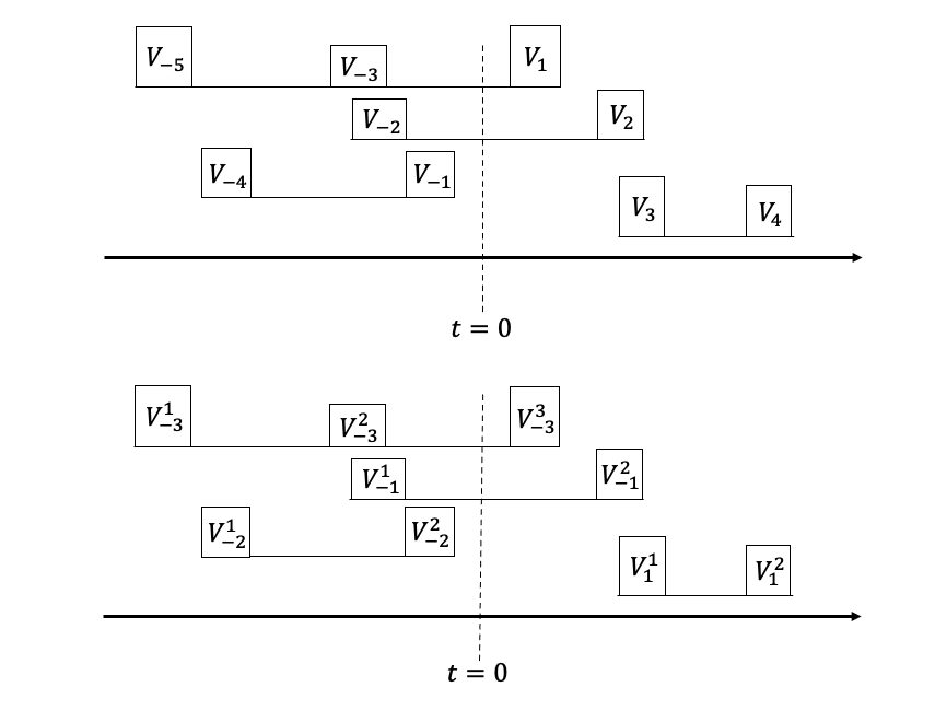
Figure 1: Illustration of the job labels. Each rectangle represents an arrival. In the top panel, the jobs are labeled according to the arrival times. In the bottom panel, the jobs are labeled by clusters.

Upon arrival, customer $n$ (or $(l,k)$) brings to the system a job of size $V_{n}$ (or $V_{l}^{k}$) which follows the distribution of a positive random variable $V$ with continuous pdf $g(\cdot)$. To include job size information, we shall write each event in $C_{l}$ as $e_{l}^{k}=(k,t_{l}^{k},p_{l}^{k},V_{l}^{k})$. Customers are served FIFO and the server processes jobs at a constant rate $\mu>0$, i.e., the service time for a customer with job size $V$ is equal to $V/\mu$. Without loss of generality, we assume that $\mathbb{E}[V]=1$.

Next, we define the queueing processes of interest. First, let $W(t)$ be the total amount of workload in the system at time $t$. Given the initial value $W(0)$, the dynamic of $W(t)$ for $t\geq 0$ can be defined as follows. Let $N(t)$ be the number of arrivals on time $[0,t)$ and define the process

$$R(t)=\sum_{n=1}^{N(t)}V_{n}-\mu t\text{ for all }t\geq 0.$$ (2)

Then, we have

$$dW(t)=dR(t)+dL(t),\text{ with }L(0)=0,\leavevmode\nobreak\ dL(t)\geq 0\text{ and }W(t)dL(t)=0.$$

Here the function $L(t)/\mu$ equals to the server’s idle time by time $t$. In addition, we have a closed-form expression for $W(t)$ for given $W(0)$ and $R(t)$:

$$W(t)=W(0)+R(t)-0\wedge\min_{0\leq s\leq t}\left\{W(0)+R(s)\right\}.$$ (3)

In addition to the workload process, we are also interested in the so-called observed busy period process $X(t)$. In particular, for any $t\geq 0$, $X(t)$ is defined as the time elapsed since the last time when the server is idle, i.e.,

$$X(t)\triangleq t-\sup\{s\leq t:W(s)=0\}.$$

We close the section by presenting the technical assumptions on the Hawkes$/GI/1$ queue. First, to ensure that the Hawkes$/GI/1$ queue is stable, we impose the following stability condition saying that the average arrival rate of jobs should be smaller than the service rate.

Assumption 1 (Stability Condition).

We assume that there exist $\varepsilon>0$ and $\underline{\mu}>0$ such that

$$\mu\in\mathcal{B}\equiv[\underline{\mu},\bar{\mu}],\quad\lambda_{0}\cdot\frac{\mathbb{E}[V]}{1-m}<\underline{\mu}-\varepsilon.$$

In addition, we also impose light-tail conditions on the birth time $b$ of the Hawkes process and individual workload $V$. These conditions will be mainly used in the proof of geometric ergodicity of the Hawkes$/GI/1$ queue.

Assumption 2 (Light-tailed Birth Time).

The birth time $b$ of the Hawkes process has a continuous density $f(\cdot)$ and finite moment generating function around $0$, i.e.

$$\psi_{b}(\theta)\equiv\mathbb{E}[\exp(\theta b)]<0,$$

for some $\theta>0$.

Assumption 3 (Light-tailed Individual Workload).

The individual workload $V$ has a finite moment generating function in a neighborhood of the origin, i.e.,

$$\psi_{V}(\theta)\equiv\mathbb{E}[\exp(\theta V)]<0.$$

4 Main Results

In this part, we present the main results on the long-run behavior of the Hawkes$/GI/1$ queue and some proof ideas. In Section 4.1 we first construct a stationary version of Hawkes$/GI/1$ queue so that we can explicitly characterize the steady-state distributions of the queueing processes. In Section 4.2, we present the finite moment results on the steady-state workload and busy periods, which are analog of the results in (Asmussen, 2003, Chapter X) for the $GI/GI/1$ model. Finally, in Section 4.3, we present the exponential ergodicity results in the form of exponentially-decay memory on the initial state and explain the coupling idea used in the proofs.

4.1 A Stationary Hawkes/GI/1 Queue

Suppose Assumption 1 holds. We shall construct a stationary version of the Hawkes/GI/1 queue following the same idea as in Loynes (1962). For a two-ended stationary Hawkes process as introduced in Section 3.2, we index the arrivals after time 0 by $n=1,2,...$, and arrivals before time 0 by $n=-1,-2,\cdots$. Recall that for all $t\geq 0$, we have defined $N(t)$ as the number of arrivals in $[0,t)$. Now, we define $N(-t)$ as the minus of the number of arrivals in $[-t,0]$. For any $t\in\mathbb{R}$ and $s\geq 0$, define

$$R^{\leftarrow}(t,s)\triangleq\sum_{n=N(t-s)}^{N(t)}V_{n}-\mu s.$$

Since the counting process $N(\cdot)$ is stationary and $V_{n}$ are i.i.d., $R^{\leftarrow}(t,\cdot)$ follows the same distribution as $R^{\leftarrow}(0,\cdot)$ for all $t\in\mathbb{R}$. Under Assumption 1, for each $t\geq 0$, $R^{\leftarrow}(t,s)$ is a process of negative drift and will go to $-\infty$ as $s\to\infty$. Therefore, we can define

$$\tilde{W}(t)\triangleq\max_{s\geq 0}R^{\leftarrow}(t,s).$$

The following proposition shows that $\tilde{W}(\cdot)$ is a stationary version of the workload process of the Hawkes$/GI/1$ queue with service rate $\mu$.

Proposition 1.

Under Assumption 1, $\{\tilde{W}(t):t\geq 0\}$ is a stationary process. Besides, the dynamic of $\tilde{W}(\cdot)$ follows the workload process of a Hawkes/GI/1 queue with customers arriving according to the stationary Hawkes process $N(t)$ with i.i.d. job sizes $V_{n}$ and served with rate $\mu$.

Similarly, we can also construct a stationary version of the observed busy period. For any $t\geq 0$, define

$$\tilde{X}(t)=\operatorname*{arg\,max}_{s\geq 0}R^{\leftarrow}(t,s).$$ (4)

Proposition 2.

The process $\tilde{X}(\cdot)$ is stationary. In addition, for each $t\geq 0$, $\tilde{X}(t)$ equals the observed busy period corresponding to the workload process $\tilde{W}(\cdot)$.

4.2 Moment of Stationary Distributions

Following the construction in Section 4.1, we shall denote the stationary workload and the stationary observed busy periods of Hawkes$/GI/1$ queue by $\tilde{W}$ and $\tilde{X}$, respectively. Our first main result is on the existence of moments and moment generating function of $\tilde{W}$ and busy time $\tilde{X}$.

Theorem 1.

Under Assumptions 1 and 2, the following statements are true.

1. If $\mathbb{E}[V_{1}^{{k+1}}]<\infty$, then $\mathbb{E}[\tilde{W}^{k}]<\infty$ and $\mathbb{E}[\tilde{X}^{k}]<\infty$.

2. In addition, if Assumption 3 holds, then

   $$\mathbb{E}[\exp(\theta_{1}\tilde{W})]<\infty,\quad\text{and}\quad{\mathbb{E}[\exp(\varepsilon\theta_{1}\tilde{X})]<\infty},$$

   where $\theta_{1}$ is a positive constant specified in (8) and $\varepsilon$ is defined in Assumption 1.

Theorem 1 is an analogue of theorem 2.1 in (Asmussen, 2003, Chapter X) and theorem 5.7 in (Asmussen, 2003, Chapter VIII). For the proof of workload, the main idea is to bound $\tilde{W}(\cdot)$ from above using an M/GI/1 queue following the idea in Chen (2021). For the proof of the busy period, we connect the busy period with the workload of another Hawkes queue but with a smaller service rate. The proof details including the construction of the $M/GI/1$ queue and the Hawkes queue with a smaller service rate will be given in Section 5.

4.3 Exponential Ergodicity of Associated Queueing Process

Our second main result is the geometric (exponential) ergodicity of the Hawkes/GI/1 queue. Following the idea in Chen et al. (2023b), we show that two Hawkes$/GI/1$ queues with different initial states can be properly coupled so that they will converge to each other exponentially fast, i.e., the dependence of the queueing process on the initial state of the system decays exponentially fast. In the setting of Hawkes$/GI/1$ queues, such dependence on the initial state can be attributed to two different sources: (i) the impact of initial congestion level in the queuing system, which is reflected by the initial values of the queueing process; (ii) the impact of Hawkes arrivals before time 0 on future arrivals. The proof method of Chen et al. (2023b) based on synchronous coupling can only deal with the first source of dependence in the setting of $GI/GI/1$. To deal with the second source of dependence that is caused by Hawkes arrivals, we shall design a new coupling called semi-synchronous coupling utilizing the cluster representation of Hawkes processes introduced in Section 3.1.

A key insight from the cluster representation is that at any time point $t$, the impact of Hawkes arrivals in the past on the future only lies in those clusters that arrive before time $t$ and depart after time $t$. To accurately describe this insight and our new coupling method, we need to introduce some extra notations. For each $t\in\mathbb{R}$, we define

$$N_{0}(t)=\{(k,t_{l}^{k},p_{l}^{k},V_{l}^{k}):(k,t_{l}^{k},p_{l}^{k},V_{l}^{k})\in C_{l},s.t.\leavevmode\nobreak\ t_{l}^{1}<t,\delta_{l}\geq t\},$$

where $\delta_{l}$ is the departure time of cluster $C_{l}$ as defined in Section 3.1. In other words, $N_{0}(t)$ is a union of all clusters that arrive before time $t$ but last after time $t$. As the clusters that arrive after time $t$ are independent of clusters that arrive before time $t$, customer arrivals after time $t$ are independent of $W(t)$ conditional on $N_{0}(t)$. We call the set $N_{0}(t)$ the Hawkes memory at time $t$. At time $0$, $N_{0}(0)$ captures all impact of Hawkes arrivals before time 0 to future arrivals, so it is natural to include $N_{0}(0)$ as part of the initial system state.

Next, we introduce two stochastic processes that are derived from $N_{0}(\cdot)$ and useful in our proofs. First, we define the total residual job size at time $t$ as

$$J_{0}(t)=\sum_{(k,t_{l}^{k},p_{l}^{k},V_{l}^{k})\in N_{0}(t),t_{l}^{k}\geq t}V_{l}^{k},$$ (5)

i.e., the total size of jobs that will arrive after time $t$ from clusters that have arrived before time $t$. Then, we define the residual life time of past history as

$$L_{0}(t)\triangleq\max\{t_{l}^{k}:(k,t_{l}^{k},p_{l}^{k},V_{l}^{k})\in N_{0}(t)\},$$

i.e., the remaining time to the last event of the past history.

Now we are ready to introduce our new coupling design for the Hawkes$/GI/1$ queue. Consider two Hawkes$/GI/1$ queues with given initial workload $W^{i}(0)$, system busy time $X^{i}(0)$ and Hawkes memories $N_{0}^{i}(0)$ for $i=1,2$. We couple two systems such that they share the same customer arrivals (including their individual workload) from the clusters that arrive after time $0$, i.e., they share the same sequence of clusters after time $0$. We call this a semi-synchronous coupling as the two systems do not exactly share the same arrivals and service times after time $0$ due to customers from $N_{0}^{1}(0)$ and $N_{0}^{2}(0)$. An illustration is given in Figure 2.

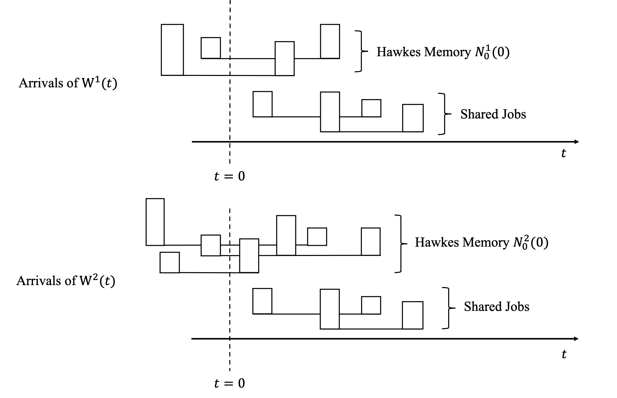
Figure 2: Illustration of semi-synchronous coupling. Each rectangle represents a job and the jobs on the same line form a cluster. The Hawkes Memories $N_{0}^{1}(0),N_{0}^{2}(0)$ are different and the clusters coming after time 0 (shared jobs) are the same.

In the Theorem 2 below, we show that two Hawkes$/GI/1$ queues that are semi-synchronously coupled will converge to each other exponentially fast. The proof is given in Section 6.

Theorem 2.

Suppose that two Hawkes/GI/1 queues with initial states $(W^{1}(0),X^{1}(0),N^{1}_{0}(0))$ and $(W^{2}(0),X^{2}(0),N^{2}_{0}(0))$ are semi-synchronously coupled and that Assumptions 1 to 3 hold. Then, there exists two positive constants $\eta,\theta>0$ such that for all $m\geq 1$

$$\mathbb{E}\left[|W^{1}(t)-W^{2}(t)|^{m}\Big{|}\mathcal{F}_{0}\right]\leq D_{0}^{m}\sum_{i=1}^{2}\exp\left(-(\eta\mu t-(\eta+2\theta)\mu L_{0}^{i}-\theta(W^{i}(0)+J^{i}_{0}(0)))_{+}\right),$$

and

$$\mathbb{E}\left[|X^{1}(t)-X^{2}(t)|^{m}\Big{|}\mathcal{F}_{0}\right]\leq\left(X^{1}(0)+X^{2}(0)+t\right)^{m}\sum_{i=1}^{2}\exp\left(-(\eta\mu t-(\eta+2\theta)\mu L_{0}^{i}-\theta(W^{i}(0)+J^{i}_{0}(0)))_{+}\right),$$

where $L_{0}^{i}(0)$ and $J^{i}_{0}(0)$ are the total residual job size and residual lifetime corresponding to $N^{i}_{0}(0)$ for $i=1,2$, respectively, and

$$D_{0}\equiv|W^{1}(0)-W^{2}(0)|+\max(J_{0}^{1},J_{0}^{2}),$$

measures the difference between the initial states $(W^{1}(0),X^{1}(0),N^{1}_{0}(0))$ and $(W^{2}(0),X^{2}(0),N^{2}_{0}(0))$.

Remark 1.

The value of constants $\eta$ and $\theta$ will be specified in (9) in Section 6. In fact, this theorem could be modified to bound

$$\mathbb{E}[f(|W^{1}(t)-W^{2}(t)|)|\mathcal{F}_{0}]$$

for any monotonic $f(\cdot)$ with $f(0)=0$ by directly replace $D_{0}^{m}$ into $f(D_{0})$ in the right-hand side.

As a direct result, we obtain exponential convergence to steady-state distribution (exponential ergodicity) for the workload process and the observed busy period process of Hawkes$/GI/1$ queue (for exponential ergodicity, see (Down et al., 1995)). Let $\mathbb{P}^{t}(\cdot|W(0),X(0),N(0))$ be the probability measure of $(W(t),X(t),N(t))$ conditional on the initial state $(W(0),X(0),N(0))$ and let $\pi$ be the stationary probability measure $\mathbb{P}^{\infty}(\cdot)$, then we have the following Corollary 1.

Corollary 1 (Exponential Ergodicity).

Under Assumption 1 to 3, we have for any initial state $(W(0),X(0),N_{0}(0))$,

$$\|\mathbb{P}^{t}\left(\cdot|\leavevmode\nobreak\ W(0),X(0),N_{0}(0)\right)-\pi\|_{TV}<\min\{e^{-\eta\mu t}(M_{0}+\exp((\eta+2\theta)\mu L_{0}+\theta(W(0)+J_{0}(0)))),1\}$$

for a constant $M_{0}>0$.

5 Proof of Theorem 1

We first introduce an auxiliary M/GI/1 queue to dominate the workload of the Hawkes/GI/1 queue in Section 5.1. Then, the analysis on the moments of steady-state workload $\tilde{W}$ and $\tilde{X}$ are given in Section 5.2 and 5.3, respectively.

5.1 An Auxiliary Dominant $M/GI/1$ Queue

We consider a single-server queue coupled with the Hawkes$/GI/1$ queue such that its customers arrive at $\{\delta_{l}:l=\pm 1,\pm 2,\cdots\}$, i.e., departure times of the clusters of the stationary Hawkes process. By reversibility, one can check that $\{\delta_{l}:l=\pm 1,\pm 2,...\}$ forms a two-ended Poisson process with rate $\lambda_{0}$ on $(-\infty,\infty)$. We let the job size brought by customer $l$ equal to

$$S_{l}\equiv\sum_{k=1}^{|C_{l}|}V_{l}^{k},\text{ for }l=\pm 1,\pm 2,...,$$

i.e., the total amount of workload brought by all customers from cluster $C_{l}$ of the Hawkes$/GI/1$ queue. Following Definition 1, $\{S_{l}\}_{l}$ is an i.i.d. sequence. In addition, by Assumption 1,

$$\lambda_{0}\mathbb{E}[S_{1}]=\lambda_{0}\frac{\mathbb{E}[V_{1}]}{1-m}<\underline{\mu}-\varepsilon<\mu.$$

Therefore, the system as described above is indeed a stable M/GI/1 queue. For all $t\in\mathbb{R}$ and $s\geq 0$, define

$$\hat{R}^{\leftarrow}(t,s)=\sum_{t-s\leq\delta_{l}<t}S_{l}-\mu s.$$

Following the same argument as in Proposition 1, this $M/GI/1$ queue has a stationary workload process

$$\hat{W}(t)=\max_{s\geq 0}\hat{R}^{\leftarrow}(t,s).$$

Similar to $J_{0}(t)$, for any $t\in\mathbb{R}$, define the backward total residual job size as

$$J^{\leftarrow}_{0}(t)=\sum_{(k,t_{l}^{k},p_{l}^{k},V_{l}^{k})\in N_{0}(t),t_{l}^{k}<t}V_{l}^{k}.$$ (6)

Then, the auxiliary $M/GI/1$ queue dominates the Hawkes$/GI/1$ queue in the following sense: the stationary workload $\tilde{W}(t)$ of the Hawkes queue can be bounded by the stationary workload $\hat{W}(t)$ of the M/GI/1 queue plus the backward total residual job size $J^{\leftarrow}_{0}(t)$.

Proposition 3.

For any $t\geq 0$,

1. $\tilde{W}(t)\leq\hat{W}(t)+J^{\leftarrow}_{0}(t)$;

2. $\hat{W}(t)$ and $J^{\leftarrow}_{0}(t)$ are independent.

5.2 Moments of the Stationary Workload

Given Proposition 3, in order to show that $\tilde{W}(0)$ has finite moment, it suffices to show that both $\hat{W}(0)$ and $J_{0}^{\leftarrow}(0)$ have finite moment. Note that $\hat{W}(0)$ is the stationary workload process of an $M/GI/1$ queue and has been extensively studied in the literature (see (Asmussen, 2003, Chapter X), (Wolff, 1989, Chapter 9) and references therein), so what remains is to bound the moments of $J_{0}^{\leftarrow}(0)$. We first introduce some technical lemmas.

Lemma 1.

There exist constants $\theta_{0},\theta_{1}>0$ such that

$$\log\psi_{b}(\theta_{0})=\log\left(\int_{0}^{\infty}\exp(\theta_{0}t)f(t)dt\right)<m-1-\log(m),$$ (7)

$$\psi_{V}(\theta_{1})<\psi_{b}(\theta_{0}/2),\quad\text{and}\quad\frac{\lambda_{0}}{\underline{\mu}{-\varepsilon}}(\psi_{S_{1}}(\theta_{1})-1)-\theta_{1}<0,$$ (8)

where $\psi_{V}$ and $\psi_{S_{1}}$ are the moment generating functions of $V_{1}$ and $S_{1}$.

Proposition 4.

Under Assumptions 1 and 2, the following statements are true.

1. If $\mathbb{E}[V^{n}]<\infty$, $\mathbb{E}[J_{0}(0)^{n}]$ and $\mathbb{E}[J_{0}^{\leftarrow}(0)^{n}]<\infty$.

2. If in addition, Assumption 3 holds, then

   $$\mathbb{E}[\exp(\theta_{1}J_{0}(0))],\quad\mathbb{E}[\exp(\theta_{1}J_{0}^{\leftarrow}(0))]<\infty,$$

   with $\theta_{1}$ specified in (8), and $\psi_{V}(\cdot),\psi_{b}(\cdot)$ being the m.g.f. of $V_{1}$ and $b$ respectively.

Now we are ready to prove that $\tilde{W}$ has finite moments and moment generating function under proper assumptions on the service time distribution. Following Proposition 3, we have

$$\tilde{W}(0)^{k}\leq\left(\hat{W}(0)+J^{\leftarrow}_{0}(0)\right)^{k}\leq 2^{k-1}\left(\hat{W}(0)^{k}+(J^{\leftarrow}_{0}(0))^{k}\right).$$

Recall that $\hat{W}(0)$ is the stationary workload process of an $M/GI/1$ queue with job size $S_{l}$ and arrival rate $\lambda_{0}$. It’s known that as long as $\mathbb{E}[S_{l}^{k+1}]<\infty$, the stationary workload $\hat{W}(0)$ has finite $k$-th moment (see theorem 2.1 in (Asmussen, 2003, Chapter X)). We compute

$$\mathbb{E}\left[S_{l}^{k+1}\right]=\mathbb{E}\left[\left(\sum_{i=1}^{|C_{l}|}V_{l}^{i}\right)^{k+1}\right]\leq\mathbb{E}[|C_{l}|^{k+1}]\mathbb{E}[V_{1}^{k+1}],$$

where the last inequality holds as $V_{k}^{l}$ are i.i.d and independent of $|C_{l}|$. Note that $|C_{l}|$ is the total number of descendants in a Poisson branching process and since $m<1$, $|C_{l}|$ follows Borel distribution, which has any finite $k$-moment (Dwass, 1969). Therefore, $\mathbb{E}[S_{l}^{k+1}]<\infty$. By Proposition 4, $\mathbb{E}[(J_{0}^{\leftarrow}(0))^{k}]<\infty$. Therefore,

$$\mathbb{E}[\tilde{W}(0)^{k}]\leq 2^{k-1}\left(\mathbb{E}[\hat{W}(0)^{k}]+\mathbb{E}[(J_{0}^{\leftarrow}(0))^{k}]\right)<\infty.$$

We next verify the workload part of statement (b). By Proposition 3, $\hat{W}(0)$ is independent of $J_{0}$. So,

$$\mathbb{E}[\exp(\theta_{1}\tilde{W}(0))]\leq\mathbb{E}[\exp(\theta_{1}\hat{W}(0)+\theta_{1}J^{\leftarrow}_{0}(0))]=\mathbb{E}[\exp(\theta_{1}\hat{W}(0))]\mathbb{E}[\exp(\theta_{1}J^{\leftarrow}_{0}(0))].$$

From Proposition 4, we have $\mathbb{E}[\exp(\theta_{1}J^{\leftarrow}_{0}(0))]<\infty$. We next show that $\mathbb{E}[\exp(\theta_{1}\hat{W}(0))]<\infty$. Notice that $\hat{W}(0)$ is the stationary workload of an $M/GI/1$ queue. Then, by transformation version of the Pollaczek-Khinchin formula (see Section 5.1.2 of Daigle (2005)),

$$\mathbb{E}[\exp(\theta_{1}\hat{W}(0))]=\frac{(1-\rho)\theta_{1}}{\theta_{1}+\frac{\lambda_{0}}{\mu}(1-\psi_{S_{1}}(\theta_{1}))}<\infty,$$

as long as $\rho\equiv\frac{\lambda_{0}}{(1-m)\mu}<1$ and $\theta_{1}+\frac{\lambda_{0}}{\mu}(1-\psi_{S_{1}}(\theta_{1}))>0$, which is guaranteed by the definition of $\theta_{1}$ in (8). As a consequence, we can conclude $\mathbb{E}[\exp(\theta_{1}\tilde{W}(0))]<\infty.$

Remark 2.

In fact, our procedure shows that under Assumption 1 to 3, any Hawkes queue with service rate $\mu\geq\underline{\mu}-\varepsilon$ has finite m.g.f in the domain $(0,\theta_{1}]$. Thus, since the $\varepsilon$ is arbitrary, we have that all moments for the stationary workload for the Hawkes queue are finite as long as the Hawkes queue is stable and the job size $V$ has a finite moment generating function around 0.

5.3 Moments of Stationary Observed Busy Period

It is known that in a stable GI/GI/1 queue, the observed busy period (in terms of how many customers served) has all finite moments under the stationary distribution (Nakayama et al., 2004) if the service times have finite moment generating function around 0. In this section, we show that a similar result holds also for the Hawkes$/GI/1$ queue but in terms of real-time. In particular, $\tilde{X}(0)$ has finite moments under certain conditions (observed busy period part of Theorem 1). However, we could not follow the analysis in Nakayama et al. (2004) due to the crucial difference between Hawkes models and the $GI/GI/1$ model.

In the proof of the moment bounds of stationary waiting time, we introduce an auxiliary $M/GI/1$ queue, and the upper bound for the $M/GI/1$ queue could give a bound for the workload of Hawkes queues. However, unfortunately, the dominant relationship of workload cannot help the observed busy period due to the existence of $J^{\leftarrow}_{0}(t)$. Our solution is to bound $\tilde{X}(0)$ by the last passage time of $\hat{R}^{\leftarrow}(0,u)$ and connect this last passage time with a stationary workload of another Hawkes queue but with a smaller service rate.

By definition, $\tilde{X}(0)=\operatorname*{arg\,max}_{u\geq 0}R^{\leftarrow}(0,u)$. Since $\max_{u\geq 0}R^{\leftarrow}(0,u)\geq 0$, then $\tilde{X}(0)$ can be bounded by the following last passage time of $R^{\leftarrow}(0,u)$,

$$\tilde{X}(0)\leq\tilde{\tau}\equiv\sup\{u\geq 0:R^{\leftarrow}(0,u)\geq 0\}.$$

Although the dominance of workload does not imply the dominance of busy time as mentioned ahead, we could find a pathwise connection between $\tilde{\tau}$ and the workload process of another Hawkes queue as follows. Recall that

$$\tilde{W}(0)=\sup_{u\geq 0}R^{\leftarrow}(0,u)=\sup_{u\geq 0}\left\{\sum_{i=-1}^{-N(-u)}V_{i}-\mu u\right\}$$

is the stationary workload of a Hawkes queue under service rate $\mu$. Similarly, we have

$$\tilde{W}_{\varepsilon}(0)\equiv\sup_{u\geq 0}\left\{R^{\leftarrow}(0,u)+\varepsilon u\right\}=\sup_{u\geq 0}\left\{\sum_{i=-1}^{-N(-u)}V_{i}-(\mu-\varepsilon)u\right\}$$

is the stationary workload of another Hawkes queue with service rate $\mu-\varepsilon$. By Assumption 1, $\tilde{W}_{\varepsilon}(0)$ is also well-defined. The following lemma connects $\tilde{\tau}$ with $\tilde{W}_{\varepsilon}(0)$.

Lemma 2.

Suppose Assumption 1 holds, then we have

$$\tilde{\tau}\leq\tilde{W}_{\varepsilon}(0)/\varepsilon$$

Proof.

Proof of Lemma 2 By definition, $R^{\leftarrow}(0,\tilde{\tau})=0$. Using this relation, we have

$$\varepsilon\tilde{\tau} =R^{\leftarrow}(0,\tilde{\tau})+\varepsilon\tilde{\tau}\leq\sup_{u\geq 0}\{R^{\leftarrow}(0,u)+\varepsilon u\}=\tilde{W}_{\varepsilon}(0).$$

Consequently, $\tilde{\tau}\leq\tilde{W}_{\varepsilon}(0)/\varepsilon$. ∎

Since $\tilde{W}_{\varepsilon}(0)$ is the stationary workload of Hawkes queue with service rate $\mu-\varepsilon$, we have proved that it has the corresponding moment bounds in Section 5.2. Then, we are ready to finish the proof of second part of Theorem 1. For statement (a), it’s clear that

$$\mathbb{E}[\tilde{X}^{k}(0)]\leq\mathbb{E}[\tilde{\tau}^{k}]\leq\mathbb{E}[\tilde{W}_{\varepsilon}(0)^{k}]/\varepsilon^{k}.$$

By the first part of Theorem 1, $\mathbb{E}[\tilde{W}_{\varepsilon}(0)^{k}]<\infty$ as long as $\mathbb{E}[V_{1}^{k+1}]<\infty$. This finishes the proof of (a).

For statement (b), following the same analysis,

$$\mathbb{E}[\exp(\varepsilon\theta_{1}\tilde{X}^{k}(0))]\leq\mathbb{E}[\exp(\varepsilon\theta_{1}\tilde{\tau})]\leq\mathbb{E}[\exp(\theta_{1}\tilde{W}_{\varepsilon}(0))]<\infty$$

where the last inequality follows the proof in Section 5.2.

6 Proof of Theorem 2 and Corollary 1

We first prove Theorem 2 in Section 6.1 and then prove Corollary 1 in Section 6.2.

6.1 Proof of Theorem 2

We first show that the difference between two semi-synchronously coupled workload processes is always bounded by the initial difference.

Lemma 3.

Suppose that two Hawkes/GI/1 queues are semi-synchronously coupled with initial states $(W^{1}(0),N_{0}^{1}(0))$ and $(W^{2}(0),N_{0}^{2}(0))$ respectively. Let $J_{0}^{i}(0)$ be the total residual job sizes in $N_{0}^{i}(0)$ for $i=1,2$. Then

$$|W^{1}(t)-W^{2}(t)|\leq|W^{1}(0)-W^{2}(0)|+\max(J_{0}^{1}(0),J_{0}^{2}(0))$$

Next, we show that two coupled workload processes $W^{1}(t)$ and $W^{2}(t)$ will eventually converge, and we can then give out the ergodic rate based on the “mixing time”. For $i=1,2$, recall that $N^{i}_{0}(0)$ is the “past history” of Hawkes processes and the $L_{0}^{i}$ is the last arrival time in $N^{i}_{0}(0)$, i.e.,

$$L_{0}^{i}=\max\{t_{l}^{k}:(k,t_{l}^{k},p_{l}^{k},V_{l}^{k})\in N_{0}^{i}(0)\}.$$

Clearly, $L_{0}^{i}$ is part of the Hawkes memory $N^{i}_{0}(0)$. Define two hitting times

$$\tau_{i}\triangleq\min\{t:W^{i}(t)=0,t\geq L_{0}^{i}\}.$$

The following lemma shows that the coupled workload processes $W^{1}(t)$ and $W^{2}(t)$ will always equal after these hitting times.

Lemma 4.

Suppose that the conditions in Lemma 3 hold. Then, for all $t\geq\max(\tau_{1},\tau_{2})$, $W^{1}(t)=W^{2}(t)$  and $X^{1}(t)=X^{2}(t)$.

Given Lemmas 3 and 4, we have, for any non-negative and non-decreasing function $f(\cdot)$ on $\mathbb{R}^{+}$ with $f(0)=0$,

$$f\left(|W^{1}(t)-W^{2}(t)|\right)\leq f\left(D_{0}\right){\bf 1}\left(\max(\tau_{1},\tau_{2})>t\right).$$

As a consequence, the analysis of the convergence rate for the Hawkes queues can be reduced to analyzing the tail probability of the hitting times $\tau_{1}$ and $\tau_{2}$. For this purpose, we have

Let

$$(\theta,\eta)=\frac{\min(\theta_{0}/2,\theta_{1})}{6\max\{\bar{\mu},1\}(\eta_{1}+2\theta_{1})}\cdot(\theta_{1},\eta_{1}),$$ (9)

with

$$\eta_{1}=\frac{1}{2}\left(\theta_{1}-\frac{\lambda_{0}}{\underline{\mu}{-\varepsilon}}(\psi_{S_{1}}(\theta_{1})-1)\right)>0.$$ (10)

Proposition 5.

Suppose that two Hawkes/GI/1 queues are semi-synchronously coupled with initial states $(W^{1}(0),X^{1}(0),N_{0}^{1}(0))$ and $(W^{2}(0),X^{2}(0),N_{0}^{2}(0))$ respectively. Let $\mathcal{F}_{0}=\sigma\left(W^{i}(0),X^{i}(0),N_{0}^{i}(0),i=1,2\right)$, then

$$\mathbb{P}(\tau_{i}>t|\mathcal{F}_{0})\leq\min\{e^{-\eta\mu t}e^{(\eta+2\theta)\mu L_{0}^{i}}e^{\theta(W^{i}(0)+J_{0}^{i}(0))},1\},$$

with $\eta$ and $\theta$ defined in (9).

Our idea is to construct two dominant $M/GI/1$ queues starting from time $L_{0}^{i}$ and estimate the hitting times of $M/GI/1$ queues by a super-martingale. Specifically, define the forward process

$$\hat{R}(t,s)=\sum_{t\leq t_{l}^{1}<t+s}S_{l}-\mu s.$$

By the same argument of Proposition 3, the forward process also has the dominance relationship by

$$R(t,s)\leq J_{0}(t)+\hat{R}(t,s).$$

Therefore, when the $M/GI/1$ queue starting from the time $L_{0}^{i}$ clears, the Hawkes/GI/1 queue must have already cleared, i.e.,

$$\tau_{i}-L_{0}^{i}\leq\hat{\tau}_{i}\equiv\min\{t\geq 0:W^{i}(L_{0}^{i})+J_{0}(L_{0}^{i})+\hat{R}(L_{0}^{i},t)=0\}.$$

To estimate $\hat{\tau}_{i}$, we define the following super-martingale

$$M_{i}(t)=\exp(\theta(W^{i}(L_{0}^{i})+J_{0}(L_{0}^{i}))+\theta\hat{R}(L_{0}^{i},t)+\eta\mu t).$$

With the help of $M_{i}(t)$, we could give an exponential moment bound of $\hat{\tau}_{i}$, which gives the hitting time distribution via Markov inequality. The full proof of Proposition 5 is in Section 10.4.

With Proposition 5, we are ready to complete the proof of Theorem 2. Recall that

$$f\left(|W^{1}(t)-W^{2}(t)|\right)\leq f\left(D_{0}\right){\bf 1}\left(\max(\tau_{1},\tau_{2})>t\right),$$

so

$$\mathbb{E}\left[f\left(|W^{1}(t)-W^{2}(t)|\right)\Big{|}\mathcal{F}_{0}\right]\leq f\left(D_{0}\right)\mathbb{P}(\max(\tau_{1},\tau_{2})>t|\mathcal{F}_{0}).$$

By Proposition 5, we can summarize that

$$\mathbb{E}\left[f\left(|W^{1}(t)-W^{2}(t)|\right)\Big{|}\mathcal{F}_{0}\right]$$

$$\leq f\left(D_{0}\right)\mathbb{P}(\max(\tau_{1},\tau_{2})>t|\mathcal{F}_{0})\leq f\left(D_{0}\right)\sum_{i=1}^{2}\mathbb{P}(\tau_{i}>t|\mathcal{F}_{0})$$

$$\leq f(D_{0})\sum_{i=1}^{2}\min\{\exp\left((\eta+2\theta)\mu L_{0}^{i}+\theta(W^{i}(0)+J^{i}_{0}(0)-\eta\mu t)\right),1\}.$$

Similarly, for the busy period, we notice that

$$|X^{1}(t)-X^{2}(t)|\leq\left(X^{1}(0)+X^{2}(0)+t\right){\bf 1}\left(\tau_{1}\vee\tau_{2}\geq t\right).$$

Therefore, by Proposition 5,

$$\mathbb{E}\left[|X^{1}(t)-X^{2}(t)\Big{|}\mathcal{F}_{0}\right] \leq\left(X^{1}(0)+X^{2}(0)+t\right)^{m}\mathbb{P}(\tau_{1}\vee\tau_{2}\geq t|\mathcal{F}_{0})$$

$$\leq e^{-\eta\mu t}\left(X^{1}(0)+X^{2}(0)+t\right)^{m}\sum_{i=1}^{2}\min\{e^{(\eta+2\theta)\mu L_{0}^{i}+\theta(W^{i}(0)+J_{0}^{i}(0))-\eta\mu t},1\}.$$

6.2 Proof of Corollary 1

To show the exponential ergodicity, we rely on our semi-synchronous coupling construction and Proposition 5. Let $W(\cdot),X(\cdot),N_{0}(\cdot)$ be the (transient) Hawkes$/GI/1$ with initial state $(W(0),X(0),N_{0}(0))$ and $(\tilde{W}(\cdot),\tilde{X}(\cdot),\tilde{N}_{0}(\cdot))$ be a stationary Hawkes$/GI/1$ queue semi-synchronously coupled with $(W(\cdot),X(\cdot),N_{0}(\cdot))$. Let $\mathcal{B}$ be the $\sigma$-field of $(W(t),X(t),N_{0}(t))$, then by definition,

$$\|\mathbb{P}^{t}(\cdot|W(0),X(0),N_{0}(0))-\pi\|_{TV}$$

$$= \sup_{A\in\mathcal{B}}|\mathbb{P}((W(t),X(t),N_{0}(t))\in A|W(0),X(0),N_{0}(0))-\mathbb{P}((\tilde{W}(t),\tilde{X}(t),\tilde{N}_{0}(t))\in A)|$$

$$\leq \mathbb{P}(W(t)\neq\tilde{W}(t),X(t)\neq\tilde{X}(t),N_{0}(t)\neq\tilde{N}(t)|W(0),X(0),N_{0}(0))$$

Note that by our construction, $(W(t),X(t),N_{0}(t))$ coincide with $(\tilde{W}(t),\tilde{X}(t),\tilde{N}(t))$ as long as $t>\max(\tau_{1},\tau_{2})$ (Lemma 4). Consequently, we have

$$\|\mathbb{P}^{t}(\cdot|W(0),X(0),N_{0}(0))-\pi\|_{TV}$$

$$\leq \mathbb{E}[\mathbb{P}(\max(\tau_{1},\tau_{2})>t|\mathcal{F}_{0})|W(0),X(0),N_{0}(0)]$$

$$\leq \min\{e^{-\eta\mu t}(M_{0}+\exp((\eta+2\theta)\mu L_{0}+\theta(W(0)+J_{0}(0)))),1\}$$

where $M_{0}=\mathbb{E}[\exp((\eta+2\theta)\mu\tilde{L}_{0}+\theta(\tilde{W}(0)+\tilde{J}_{0}(0)))]<\infty$. The last inequality is by Proposition 5.

7 Application Example: Online Learning for Hawkes/GI/1 Queue

In this section, we introduce an application of the theory developed in Section 4. Specifically, we introduce an online learning problem for Hawkes$/GI/1$ queues and design the first online learning algorithm for the staffing problem of Hawkes$/GI/1$ queues. In addition, we analyze the efficiency of this algorithm via the regret analysis and the convergence rate of the algorithm, the heart of which is the moment bounds and the ergodicity results in Section 4.

7.1 Problem Setting and Assumptions

We consider a Hawkes/GI/1 queue in which the customers arrive following a stationary Hawkes process with unknown parameter $(\lambda_{0},m,f(\cdot))$ and the i.i.d. job size follows a positive random variable $V$ with mean $1$ with service rate $\mu$ as in Section 3. In the staffing problem, the service provider’s goal is to find the best choice of $\mu\in\mathcal{B}=[\underline{\mu},\bar{\mu}]$ to balance between the staffing cost (per unit time) and the penalty of congestion:

$$\min_{\mu\in\mathcal{B}}f(\mu)\equiv h_{0}\mathbb{E}[W_{\infty}(\mu)]+c(\mu),$$ (11)

where $W_{\infty}(\mu)$ is the steady-state workload process under the staffing level $\mu$ and $c(\mu)$ is the corresponding staffing cost. For the ease of notation, let’s denote $w(\mu)\triangleq\mathbb{E}[W_{\infty}(\mu)]$. We shall additionally impose the following assumption for the rest of this article to guarantee the convexity of the objective, which is a common practice in online learning literature (Hazan et al., 2016).

Assumption 4 (Service Cost).

We assume the staffing cost function $c(\mu)$ is convex, continuously differentiable and non-decreasing in $\mu$.

The form of the staffing problem (11) has a long history in traditional queueing systems (see, for example, (Maglaras and Zeevi, 2003; Lee and Ward, 2014; Nair et al., 2016; Chen et al., 2023b) and references therein). However, in problem (11), the workload $\mathbb{E}[W_{\infty}(\mu)]$ has no closed form even for $GI/GI/1$ queue, let alone more complicated Hawkes$/GI/1$ queue, so the problem (11) is intractable analytically. Therefore, we design the first online learning algorithm for the Hawkes staffing problem (11) without knowledge of the information of Hawkes arrivals (to the best of our knowledge).

7.2 Online SGD-Based Algorithm and the System Dynamics

In this section, we introduce our algorithm designed for the Hawkes$/GI/1$ queue. Our algorithm is designed based on the framework of Gradient-based Online Learning in Queues (GOLiQ) algorithm in our recent paper Chen et al. (2023b), which is an algorithm specially designed for $GI/GI/1$ queue for a similar problem. Although we could not directly apply GOLiQ to the Hawkes system due to the difference between Hawkes queues and $GI/GI/1$ queue, our moment bound and ergodicity results in Section 4 provide us the key ingredients to design and efficiency analysis of the new algorithm (Algorithm 1

Algorithm 1 Online Algorithm for Hawkes$/GI/1$ Queues (GOLiQ-Hawkes)

1:number of cycles $L$, parameters $T_{k}$, $\eta_{k}$ for $k=1,2,...,L$, initial value $\mu_{1}$, warm-up rate $\xi$

2:for $n=1,2,...,L$ do

3:     operate the system under $\mu_{k}$ until time $T_{k}$

4:     observe $X_{k}(t)$ for $t\in[0,T_{k}]$

5:     estimate gradient by

$$H_{k}=-\frac{h_{0}}{(1-\xi)T_{k}}\int_{\xi T_{k}}^{T_{k}}X_{k}(t)dt+c^{\prime}(\mu)$$

6:     update: $\mu_{k+1}=\min\left(\max(\mu_{k}-\eta_{k}H_{k},\underline{\mu}),\bar{\mu}\right)$

7:end for

Our algorithm falls into the category of gradient descent method. In our algorithm, we organize the time into successive cycles according to the hyperparameter $T_{k}$, the cycle length. To mitigate the bias introduced by the transient state of the queue, the algorithm sends $T_{k}$ to $\infty$ as $k\rightarrow\infty$. In each cycle, the algorithm operates the system under $\mu_{k}$ and builds a gradient estimator $H_{k}$ with data collected within the cycle. At the end of the cycle, the system updates $\mu_{k+1}$ by an SGD rule. Due to the cyclic design, we use the under-script _k to denote the corresponding stochastic process in cycle $k$, e.g., $N_{k}(t),W_{k}(t),X_{k}(t),J_{0,k}(t)\cdots$ being the corresponding arrival, workload, busy time, total residual job sizes, etc., in cycle $k$.

The heart of Algorithm 1 is its gradient estimator. In our case, the challenge is to estimate $w^{\prime}(\mu)$, which has no closed form, from data without involving any unknown Hawkes information, i.e., the parameters $(\lambda_{0},m,f)$. For this purpose, we apply a pathwise analysis to the Hawkes system and derive a convenient expression of the derivative of $w(\mu)$ by the following representation theorem.

Proposition 6.

Suppose Assumption 1 holds. Then, for a $Hawkes/GI/1$ queue with stationary input, the derivative of the mean steady-state workload $w(\mu)$ satisfies

$$w^{\prime}(\mu)=-\mathbb{E}[X_{\infty}(\mu)],$$

where $X_{\infty}$ is the steady-state of the observed busy period (in continuous time) for $\mu\in\mathcal{B}$. Moreover, $w(\mu)$ is Lipchitz continuous for $\mu\in\mathcal{B}$, i.e.,

$$|w(\mu_{1})-w(\mu_{2})|\leq\mathbb{E}\left[X_{\infty}(\underline{\mu})\right]|\mu_{1}-\mu_{2}|.$$

With this gradient representation, we apply a finite time sample average in each cycle to estimate the gradient in Algorithm 1. The key of Proposition 6 is to analyze the gradient pathwisely. In detail, by the construction in Section 5, we could prove that almost surely,

$$\tilde{W}_{\mu}(0)^{\prime}=\left(\max_{u\geq 0}R_{\mu}^{\leftarrow}(0,u)\right)^{\prime}=-\tilde{X}_{\mu}(0).$$

Therefore, once we can interchange the derivative and the expectation, then Proposition 6 is at hand and the interchange could be guaranteed by the moment condition in Theorem 1. For more details, see the full proof in Section 10.5.3.

7.3 Regret Analysis

In this section, we show the efficiency of GOLiQ-Hawkes by providing corresponding performance bounds. Specifically, we consider the regret as the performance measure, which is commonly used in online learning literature, e.g., Hazan et al. (2016) and references therein. In a nutshell, regret is the difference between the performance of the system under the online learning algorithm and the performance under the optimal staffing level $\mu^{*}$. In detail, the regret accumulated in cycle $k$ is defined by

$$R_{k}=\underbrace{\mathbb{E}\left[c(\mu_{k})T_{k}+h_{0}\int_{0}^{T_{k}}W_{k}(t)dt\right]}_{\text{the cumulative cost in cycle $k$}}-\underbrace{f(\mu^{*})T_{k}}_{\text{the optimal cost}}.$$ (12)

As a result, the total regret in $L$ cycles is $R(L)=\sum_{k=1}^{L}R_{k}$.

Although we could not directly apply the analysis of GOLiQ to GOLiQ-Hawkes due to the differences between Hawkes arrivals and renewal arrivals, the analysis framework of GOLiQ in Chen et al. (2023b) sheds some light on the analysis of GOLiQ-Hawkes. Essentially, the success of GOLiQ is substantiated by (i) the boundedness of key queueing functions in each cycle; (ii) the geometric ergodicity of $GI/GI/1$ queue; and (iii) the convex structure of the revenue management objective. In other words, if we could provide the parallel conditions of (i) to (iii) ahead in the Hawkes version, GOLiQ-Hawkes would have an efficient convergence rate as GOLiQ does. Fortunately, our results in Section 4 provide these properties adapted to Hawkes queue’s version. We summarize these three properties as follows and note that these properties are direct results of our analysis in Section 4. The proofs of these properties are collected in Appendix Section 10.5.

Corollary 2 (Boundedness of Queueing Functions).

Suppose Assumption 1 to 3 hold. For any control sequence $\mu_{k}\in\mathcal{B}$, with

$$(\theta,\eta)=\frac{\min(\theta_{0}/2,\theta_{1})}{6\max(\bar{\mu},1)(\eta_{1}+2\theta_{1})}\cdot(\theta_{1},\eta_{1})$$

as defined in (9), the following queueing terms

$$\mathbb{E}[W_{k}(t)^{2m}],\mathbb{E}[X_{k}(t)^{2m}],\mathbb{E}[J_{0,k}(t)^{2m}],\mathbb{E}[e^{6(\eta+2\theta)\mu_{k}L_{0,k}}],\mathbb{E}[e^{6\theta W_{k}(t)}],\mathbb{E}[e^{6\theta J_{0,k}(t)}]$$

are bounded by a constant $M$.

Corollary 3 (Ergodicity of Queueing Functions in Each Cycle).

Suppose that Assumption 1 to 3 hold. Let $\tilde{W}_{k}(t)$ be a stationary workload process semi-synchronously coupled with $W_{k}(t)$. In addition, let $X_{k}(t),\tilde{X}_{k}(t)$ be the corresponding busy time. Then, there exists a constant $A$ such that for $m=1,2$,

$$\mathbb{E}\left[\left|W_{k}(t)-\tilde{W}_{k}(t)\right|^{m}\right] \leq Ae^{-\eta\underline{\mu}t}$$

$$\mathbb{E}\left[\left|X_{k}(t)-\tilde{X}_{k}(t)\right|^{m}\right] \leq Ae^{-0.5\eta\underline{\mu}t},$$

where $\eta$ is specified in (9).

Corollary 4 (Convex and Smoothness).

Suppose Assumption 1 to 4 hold. The objective function $f(\mu)$ has a continuous first-order derivative denoted by $\nabla f(\mu)$. There exist finite positive constants $K_{0}\leq 1$ and $K_{1}>K_{0}$ such that for all $\mu\in\mathcal{B}$

1. $(\mu-\mu^{*})\nabla f(\mu)\geq K_{0}(\mu-\mu^{*})^{2}$

2. $|\nabla f(\mu)|\leq K_{1}|\mu-\mu^{*}|$

Armed by the boundedness, exponential ergodicity and convex property, the efficiency of GOLiQ-Hawkes could be summarized by the following theorem. In short, we will show that with properly chosen hyper-parameters $\eta_{k}$ and $T_{k}$, GOLiQ-Hawkes is efficient in the sense that it has a logarithmic regret, which also indicates that the decision $\mu_{k}$ of GOLiQ-Hawkes will also converge to the clairvoyant policy $\mu^{*}$ in a rapid speed.

Theorem 3.

Under Assumption 1 to 4, let $T_{k}=a_{T}+c_{T}\log(k)$, $\eta_{k}=c_{\eta}k^{-1}$ with any

$$c_{T}\geq 2(\eta\underline{\mu}\xi)^{-1}\max(\log(8A/K_{0}),1),\quad\text{and}\quad c_{\eta}\geq 2k^{-1}/K_{0},$$

and any $a_{T}\geq 0$, where $\eta$ is specified in (9), $\xi$ is the warm-up rate in Alg.1, $A$ is defined in Corollary 3, and $K_{0}$ is the strong convexity constant in Corollary 4. Then there exists a constant $C_{alg}>0$ such that, for all $L\geq 1$,

$$R(L)\leq C_{alg}\log(L)^{2}.$$

In particular, we have

$$R(L)=O(\log(L)^{2})=O(\log(M_{L})^{2}),$$

with $M_{L}=\sum_{k=1}^{L}T_{k}$, i.e., the total units of time elapsed in $L$ cycles.

Remark 3.

Compared to conventional $\log(L)$ regret for online gradient descent Hazan et al. (2016), the additional logarithm comes from the transient behavior of the Hawkes queues and the exponential convergence rate of Hawkes queues.

With the three critical properties of Hawkes queues, the efficiency of GOLiQ-Hawkes could be provided following the analysis framework of Chen et al. (2023b). Basically, the key idea of the analysis is to decompose the regret into the following two parts:

$$R_{1,k} =\mathbb{E}\left[h_{0}\int_{0}^{T_{k}}W_{k}(t)-w(\mu_{k})dt\right]$$

$$R_{2,k} =\mathbb{E}\left[f(\mu_{k})-f(\mu^{*})\right]T_{k}.$$

Then the total regret cumulated in $L$ cycles is decomposed accordingly as

$$R(L)=\sum_{k=1}^{L}R_{k}=\sum_{k=1}^{L}R_{1,k}+\sum_{k=1}^{L}R_{2,k}\triangleq R_{1}(L)+R_{2}(L).$$

Intuitively, $R_{1}(L)$ is the regret caused by transient behavior of the queueing system (regret of the transient behaviors). On the other hand, $R_{2}(L)$ can be interpreted as the regret driven by suboptimality of the decision variable $\mu_{k}$ (regret of suboptimality). For the regret of transient behaviors $R_{1}$, we could apply the exponential ergodicity result. The regret of suboptimality $R_{2}$ hinges on the bias and variance of the gradient estimator $H_{k}$. We analyze the bias by ergodicity and the variance by boundedness. With the help of convexity, the regret of suboptimality $R_{2}$ can be well controlled, too. For the sake of brevity, we would like to omit the full proof here and defer the full proof in the Appendix Section 10.5.3.

8 Numerical Results

In this section, we first confirm the effectiveness of GOLiQ-Hawkes via numerical experiments. Then we investigate the impact of autocorrelation of the Hawkes process on the staffing decision by comparing it with a $GI/GI/1$ queue with same marginal inter-arrival time distribution. Finally, we study the optimal staffing in a heavy-traffic regime to see whether the classic “square-root rule” still holds for Hawkes queues. In all numerical experiments, the stationary Hawkes arrivals is generated using the perfect sampling algorithm 1 developed in Chen (2021).

8.1 Performance Evaluation of GOLiQ-Hawkes

We consider problem (11) with a quadratic staffing cost $c(\mu)=c_{0}\mu^{2}$ in this section. In specific, we set $h_{0}=c_{0}=0.5$. As a result, the objective (11) reduces to

$$\min_{\mu\in\mathcal{B}}f(\mu)=\min_{\mu\in\mathcal{B}}\left\{0.5\mu^{2}+0.5\mathbb{E}\left[W_{\infty}(\mu)\right]\right\}.$$ (13)

Since there is no closed form of $\mathbb{E}[W_{\infty}(\mu)]$, the exact solution $\mu^{*}$ of problem (13) is unavailable. We apply the naive grid search method (NGS) and set the solution of NGS as the benchmark for regret estimation. In detail, for each candidate $\mu$, we operate Hawkes$/GI/1$ queues under $\mu$ for $T=100,000$ unit times and estimate $\mathbb{E}[W_{\infty}(\mu)]$ by time average estimator $\frac{1}{0.5T}\int_{0.5T}^{T}W(t)dt$. The estimate $\hat{f}(\mu)$ is achieved based on $100$ independent time averaging estimations above. By comparing all $\hat{f}(\mu)$, we choose $\mu$ with the smallest $\hat{f}(\mu)$ as yardstick $\mu^{*}$, with which we are able to benchmark the solutions of GOLiQ-Hawkes.

We consider non-Markovian Hawkes arrivals with unit background intensity $\lambda_{0}=1$ and Gamma kernel $m(t)=2te^{-2t}$. In this case, $m=\int_{0}^{\infty}m(t)dt=1/2$, and the average arrival rate $\lambda=2$. For service times, we consider Erlang-2 distribution with a rate of $2\mu$. The NGS method gives out the benchmark that $\hat{\mu}^{*}=2.84$ and $\hat{f}(\mu^{*})=6.11$ (with a precision of 0.01), and the cost function is shown in the top left panel of Figure 3 as well. By Algorithm 1 and Theorem 3, we select step length $\eta_{k}=1/k$ and cycle length $T_{k}=10+20\log(k)$ with initial point $\mu_{0}=10$. In Figure 3, we again give a sample path of staffing level $\mu_{k}$ and the estimated regret curve (obtained by 1,000 independent Monte-Carlos runs). We find that the staffing level $\mu_{k}$ converges to the optimal value $\mu^{*}$ rapidly, and the regret grows as a logarithmic function of time $t$. Particularly, a simple linear regression with respect to $\left(\sqrt{R(t)},\log(t)\right)$ (bottom right panel) validates our regret bound in Theorem 3.

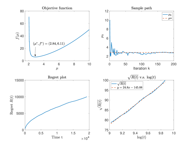
Figure 3: Online optimal staffing for non-Markovian Hawkes$/GI/1$ by GOLiQ-Hawkes with $\mu^{*}=2.84$, $\eta_{k}=1/k$ and $T_{k}=10+20\log(k)$: (i) objective function (top left); (ii) sample path of the staffing level $\mu_{k}$ (top right); (iii) estimated regret (bottom left); (iv) square root of regret versus logarithmic of the total time elapsed (bottom right).

We further test the robustness of GOLiQ-Hawkes by applying different hyperparameters $\eta_{k}$ and $D_{k}$. Specifically, we first validate the robustness of $\eta_{k}$ by choosing $\eta_{k}=c_{\eta}k^{-1}$ with $c_{\eta}\in\{0.5,1,3,5\}$ and fixing $T_{k}=10+20\log k$. Next, we verify the robustness of $T_{k}$ by selecting $T_{k}=10+c_{T}\log k$ with $c_{T}\in\{10,20,30\}$ and fixing $\eta_{k}=k^{-1}$. For each case, the regret curve is estimated by 1,000 independent runs, and in Figure 4, we also draw $\sqrt{R(t)}$ v.s. $\log(t)$ plot. Figure 4 reveals that GOLiQ-Hawkes continues to perform efficiently with different hyperparameters with all regret curves exhibiting a logarithmic order. In summary, our numerical experiments illustrate that GOLiQ-Hawkes performs effectively with a logarithmic regret and that GOLiQ-Hawkes is robust to the hyperparameter choices.

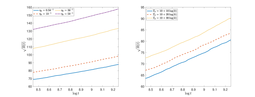
Figure 4: Simulated $\log t$ v.s. $\sqrt{R(t)}$ plot with different hyperparameters (i) step size $\eta_{k}$ robustness (left panel); (ii) cycle length $T_{k}$ (right panel). All regret curves are estimated by averaging 1,000 independent replications.

8.2 Impact of Self-excitement of Hawkes arrivals

In this section, we conduct numerical experiments to investigate the impact of the self-excitement of Hawkes arrivals on the optimal stuffing level $\mu^{*}$. Specifically, we compare the optimal staffing level between queueing systems with Hawkes arrivals and systems with renewal arrivals, of which the interarrival times have the same distribution as the marginal distribution of the stationary Hawkes process’ interarrival times.

For this purpose, we generate the arrival process $(GI)$ by the following shuffling method: (i) we first generate a sufficiently long stationary Hawkes process’s path; (ii) all of the interarrival times of this Hawkes path are randomly shuffled; (iii) the ideal $GI$ renewal process is generated by splicing these shuffled interarrival times. Then GOLiQ-Hawkes is applied to both the Hawkes$/GI/1$ queue and the corresponding $GI/GI/1$ queue to obtain the optimal level $\mu_{H}^{*}$(the optimal staffing for Hawkes queue) and $\mu_{GI}^{*}$ (the optimal level for $GI/GI/1$ queue).

Since we intend to investigate the impact of the autocorrelation on optimal staffing, we compare $\mu_{H}^{*}$ with $\mu_{GI}^{*}$ under different autocorrelation levels for objective (13). A convenient indicator of autocorrelation level for Hawkes process is $m=\int_{0}^{\infty}m(t)dt$, i.e., the average number of offspring of a single arrival. Therefore, in this experiment, we consider kernels in the form:

$$m(t)=a\cdot e^{-2t},\quad a\in\{0,0.2,\cdots,1.8\},$$

so that $m=\{0,0.1,\cdots,0.9\}$. As higher autocorrelation level results in a larger arrival rate, to make experiments comparable, the background intensity $\lambda_{0}$ is chosen as $\lambda_{0}=2\cdot(1-m)$ accordingly so that the total arrival rate $\lambda=\frac{\lambda_{0}}{1-m}=2$ across all the cases. In this way, we have a sequence of systems whose total arrival rates are the same but the auto-correlation level increases with $m$. As for the service distribution, we consider exponential service times for simplicity. Then, we investigate the impact of the auto-correlation level of the Hawkes process by comparing the difference of $\mu^{*}_{GI}$ and $\mu^{*}_{H}$ under different auto-correlation level $m$ in each case.

For each case, we apply the GOLiQ-Hawkes for $L=300$ iterations for $100$ independent replications. The $\mu_{\text{Hawkes}}^{*}$ and $\mu_{\text{GI}}^{*}$ is estimated by averaging the staffing level in the last iteration, i.e., $\mu_{L}$ of the $100$ independent paths. The hyperparameters for GOLiQ-Hawkes in both Hawkes queue and $GI/M/1$ queue are $\eta_{k}=3/k,T_{k}=10+20\log(k)$. The results are reported in Table 1.

m	Hawkes/M/1		GI/M/1		Relative Increase in $\mu^{*}$
	$\mu_{H}^{*}$	Variance	$\mu_{GI}^{*}$	Variance
0	2.61	0.0014	2.61	0.0016	0.00%
0.1	2.64	0.0019	2.62	0.0015	0.64%
0.2	2.68	0.0019	2.65	0.0014	1.13%
0.3	2.72	0.0017	2.66	0.0016	2.24%
0.4	2.80	0.0028	2.70	0.0021	3.88%
0.5	2.90	0.0027	2.74	0.0013	5.56%
0.6	3.05	0.0039	2.79	0.0026	9.12%
0.7	3.27	0.0066	2.87	0.0016	14.05%
0.8	3.70	0.0130	3.03	0.0034	22.14%
0.9	4.62	0.0583	3.40	0.0052	35.97%

Table 1: The estimated value and variance of optimal service capacity solved by GOLiQ-Hawkes for 100 replications for Hawkes$/M/1$ and the corresponding $GI/M/1$ with different levels of self-excitement $m$.

Table 1 illustrates that as the autocorrelation level $m$ grows, both Hawkes$/M/1$ and $GI/M/1$ queues need higher staffing levels to accommodate the surge of arrivals. However, the Hawkes$/M/1$ queue needs significantly more service capacity than the $GI/M/1$ queue due to Hawkes’ autocorrelation at all levels of $m$. In addition, the relative difference in staffing levels, i.e.,

$$\frac{\mu_{H}^{*}-\mu_{GI}^{*}}{\mu_{GI}^{*}}$$

grows with $m$, which implies that the difference between Hawkes queues and $GI/GI/1$ queues inclines to be sharper as the autocorrelation level increases, and consequently, the Hawkes$/GI/1$ queue needs significantly more service capacity as Hawkes’ autocorrelation level increases.

8.3 Does “square root rule” hold for Hawkes queues?

The square root rule is prevalent in many queueing models for determining the optimal staffing level. Specifically, Lee and Ward (2014) proved asymptotic optimality of the square root rule for $GI/GI/1$ queue with linear staffing cost, i.e. the optimal staffing level satisfies

$$\mu^{*}=\lambda+O(\sqrt{\lambda}),\quad\text{as }\lambda\rightarrow\infty.$$

To check whether the square root rule still holds for Hawkes$/GI/1$ queue, we design a set of numerical experiments as follows. We consider the staffing problem with linear cost as

$$\min_{\mu}2\mu+0.1\mathbb{E}[W_{\infty}(\mu)]$$

on a set of Hawkes$/GI/1$ queues with same exponential service time distribution but with increasing avaerage intensity $\lambda$ in the Hawkes arrival processes. We then observe how the optimal staffing level $\mu^{*}_{H}$ changes with $\lambda$ and whether it increases following the square root rule. As a comparison, we also solve the same staffing problem for a $GI/GI/1$ queue with IID inter-arrival times follow the same marginal distribution as that of Hawkes queue constructed in the same way as described in Section 8.2.

As the major difference lies in autocorrelation, we send the arrival rate $\lambda$ to infinity by letting $m\rightarrow 1$. In specific, we consider a sequence of Hawkes queueing systems indexed by $n$ with the same background intensity $\lambda_{0}=1$. However, the kernel of the Hawkes process in each system changes with $n$ in the form of $m(t)=(2-2/n)e^{-2t}$ so that the total arrival rate

$$\lambda=\frac{\lambda_{0}}{1-m}=n$$

in the $n$-th system. In the experiment, we consider $n\in\{5,25,45,65,85,105\}$. We investigate how $\mu^{*}_{H}$ and $\mu^{*}_{GI}$ change with $n$ and whether they obey the square root rule.

To derive the solutions $\mu^{*}_{H}$ and $\mu^{*}_{GI}$, in each case, we apply GOLiQ-Hawkes to both Hawkes$/GI/1$ and $GI/GI/1$ systems by 100 replications, and the optimal levels are estimated in the same procedure in Section 8.2 with the same hyperparameters. If the square root rule still holds for Hawkes$/GI/1$ queue, then $\mu_{H}^{*}-\lambda$ shall be linear with $\sqrt{\lambda}$ and the ratio between them shall be close to a constant. The results are reported in Table 2.

In Table 2, we report the total arrival rate, the average number of descendants $m$, the auto-correlation function (ACF) with lag-1 and the estimated $\mu^{*}_{H}$ (and $\mu^{*}_{GI}$). From Table 2, we can observe that as $m$ increases, $\lambda$ and ACF increase at the same time, which results in the increase of both staffing levels $\mu_{H}^{*}$ and $\mu_{GI}^{*}$. Parallel to the experiment in Section 8.2, the need for staffing in Hawkes queues $\mu^{*}_{H}$ is always larger than the staffing in renewal case $\mu^{*}_{GI}$. In addition, the difference between Hawkes queue and $GI/GI/1$ queue is quite sharp because a mild autocorrelation (ACF$=0.401$) may lead to $50\%$ more staffing! And the difference seems to enlarge with the increase of $\lambda$.

In addition, we can observe in Table 2 that, as $\lambda$ increases, the ratio $\frac{\mu^{*}_{H}-\lambda}{\sqrt{\lambda}}$ increases dramatically in Hawkes queue, while for $GI/GI/1$ queue, the ratio $\frac{\mu_{GI}^{*}-\lambda}{\sqrt{\lambda}}$ is around the same level of 0.35. In other words, this result confirms that the square-root rule works for $GI/GI/1$ queue but not for the Hawkes$/GI/1$ queue especially when the increasing of average arrival rate is driven by the self-excitement effect, i.e. $m\to 1$. We leave theoretic justification on this result for further study.

$\lambda$	$m$	ACF	Hawkes/$GI/1$			$GI/GI/1$
			$\mu^{*}_{H}$	$\rho^{*}_{H}$	$\frac{\mu^{*}_{H}-\lambda}{\sqrt{\lambda}}$	$\mu^{*}_{GI}$	$\rho^{*}_{GI}$	$\frac{\mu^{*}_{GI}-\lambda}{\sqrt{\lambda}}$
5	0.800	0.235	6.16	0.812	0.52	5.78	0.865	0.35
25	0.960	0.331	33.6	0.744	1.72	26.7	0.936	0.34
45	0.978	0.349	63.4	0.709	2.74	47.2	0.953	0.33
65	0.985	0.354	95.7	0.680	3.81	67.8	0.959	0.35
85	0.988	0.362	131.2	0.648	5.01	88.4	0.962	0.37
105	0.991	0.401	166.4	0.631	5.99	109	0.967	0.35

Table 2: The estimated $\mu^{*}$ for Hawkes$/M/1$ queues and $GI/M/1$ queues with different $\lambda$.

9 Conclusion

In this paper, we establish moment bounds and exponential ergodicity for the general Hawkes$/GI/1$ queues under the stability condition. The key challenge in our analysis lies in the fact that the initial state of the Hawkes system contains the information of future arrivals and hence, the conventional approach is not applicable. To remedy this issue, we develop a semi-synchronous coupling method decomposing the future arrivals into two parts and we deal with them in different manners, which, we believe, is of independent research interest and can be useful for other stochastic models related to Hawkes processes. As an application of the theoretic results, we develop an efficient numerical tool for solving the optimal staffing problems in Hawkes$/GI/1$ queue. Our numerical results document the significant impact of clustering or auto-correlation in the arrival processes on decision-making of staffing service systems.

There are several venues for future research. Since we show numerically that the square-root rule is not always satisfactory for Hawkes queues, one natural direction is to theoretically verify the numerical finding and identify the correct asymptotic staffing rule. Another interesting dimension is to investigate Hakwes queues with long-tail excitation function and possibly heavy tailed service times.

APPENDIX

10 Proofs

In this section, we give the proofs of auxiliary results in the main paper.

10.1 Proof of Auxiliary Results in Section 3

Proof.

Proof of Lemma 1 Since $0<m<1$ as assumed, we have $m-1-\log(m)>0$. As a result, there exists $\theta_{0}$ such that $0<\log\mathbb{E}[\exp(\theta_{0}b)]<m-1-\log(m)$. Note that if moment generating function exists around $0$, then it’s continuous differentiable in its domain (Mood et al., 1974, p.78). Therefore, for (8), since $\psi_{V}(\cdot)$ is smooth around $0$, we have $\psi_{S_{1}}(\theta)=\psi_{|C_{1}|}(\log\psi_{V}(\theta))$ is also smooth around $0$. In this case, we can find a $\theta_{1}$ satisfying (8) as follows. Since $\psi_{V}(\cdot)$ is smooth around $0$, then there exists a $\theta_{0}^{\prime}$ such that $\psi_{V}(\theta_{0}^{\prime})<\psi_{b}(\theta_{0}/2)$. For the other condition, define an auxiliary function

$$h(\theta)=\quad\frac{\lambda_{0}}{\underline{\mu}-{\varepsilon}}(\psi_{S_{1}}(\theta)-1)-\theta.$$

By direct calculation, $h(0)=0,h^{\prime}(0)=\frac{\lambda_{0}}{(1-m)(\underline{\mu}-{\varepsilon})}<0$ and $h^{\prime\prime}(\theta)=\frac{\lambda_{0}}{\underline{\mu}-{\varepsilon}}\psi_{S_{1}}^{\prime\prime}(\theta)=\frac{\lambda_{0}}{\underline{\mu}-{\varepsilon}}\mathbb{E}[S_{1}^{2}e^{\theta S_{1}}]>\frac{\lambda_{0}}{\underline{\mu}-{\varepsilon}}\mathbb{E}[S^{2}]>0$ for any $\theta>0$. Therefore, there exists one and only one positive solution for $h(\bar{\theta})=0$, and denote it by $\bar{\theta}$. Clearly, $h(\theta)<0$ for $\theta\in(0,\bar{\theta})$. Then, we can choose

$$\theta_{1}=\min(\theta_{0}^{\prime},\bar{\theta}/2),$$

which satisfies (8). ∎

10.2 Proofs of the Auxiliary Result in Section 4.1 and 5.1

Proof.

Proof of Proposition 1Under Assumption 1, for any $t\geq 0$, the process $R^{\leftarrow}(t,s)\to-\infty$ almost surely as $s\to\infty$. As a consequence, $\tilde{W}(t)$ is well-defined. In addition, for any $t$, the process $R^{\leftarrow}(t,\cdot)$ follow the same distribution as $R^{\leftarrow}(0,\cdot)$. So $\tilde{W}(t)$ has the same distribution as $\tilde{W}(0)$ for all $t\geq 0$, and hence is stationary.

Now we show that $\tilde{W}(\cdot)$ follows the dynamic of a workload process of a Hawkes/GI/1 queue. Note that $\tilde{W}(0)$ is the initial workload, customers arrive according to $N(t)$ with i.i.d. job size $V_{n}$, and service rate is $\mu$. For any $t\geq 0$ and $s>t$,

$$R^{\leftarrow}(t,s) =\sum_{n=N(t-s)}^{N(t)}V_{n}-\mu s$$

$$=\sum_{n=N(t-s)}^{-1}V_{n}-\mu(s-t)+\sum_{n=1}^{N(t)}V_{n}-\mu t$$

$$=R^{\leftarrow}(0,s-t)+R(t).$$

As a consequence,

$$\max_{s\geq t}R^{\leftarrow}(t,s)=\max_{s\geq 0}R^{\leftarrow}(0,s)+R(t)=\tilde{W}(0)+R(t).$$

Recall that $R(t)$ is defined in (2). For $0\leq s\leq t$, we have

$$R^{\leftarrow}(t,s)=R(t)-R(0,t-s).$$

Then,

$$\tilde{W}(t) =\max_{s\geq 0}R^{\leftarrow}(t,s)=\left(\tilde{W}(0)+R(t)\right)\vee\max_{0\leq s\leq t}(R(t)-R(s))$$

$$=R(t)-(-\tilde{W}(0))\wedge\min_{0\leq s\leq t}(R(s))$$

$$=\tilde{W}(0)+R(t)-0\wedge\min_{0\leq s\leq t}\left\{\tilde{W}(0)+R(s)\right\}.$$

According to (3), we can conclude that $\tilde{W}(t)$ has the same dynamics as the of a Hawkes/GI/1 queue in which customers arrive according to the stationary Hawkes process $N(t)$ with i.i.d. job sizes $V_{n}$ and are served with rate $\mu$. ∎

Proof.

Proof of Proposition 2 For convenience, define $t_{0}=t-\tilde{X}(t)$. Then,

$$\tilde{W}(t_{0}) =\max_{s\geq 0}R^{\leftarrow}(t_{0},s)$$

$$=\max_{s\geq 0}R^{\leftarrow}(t,t-t_{0}+s)-R^{\leftarrow}(t,t-t_{0})$$

$$=\max_{s\geq 0}R^{\leftarrow}(t,t-t_{0}+s)-R^{\leftarrow}(t,\tilde{X}(t))\leq 0.$$

Since $\tilde{W}(t)\geq 0$, we have $\tilde{W}(t_{0})=0$. Similarly, if there is a $t_{1}$ such that $t_{0}<t_{1}\leq t$, and $\tilde{W}(t_{1})=0$, then

$$R^{\leftarrow}(t,t-t_{1})\geq R^{\leftarrow}(t,t-t_{0}),$$

which is impossible by definition of $\tilde{X}(t)$ and $t_{0}$. So $t_{0}=\sup\{s\leq t:\tilde{W}(s)=0\}$. This finishes the proof. ∎

Proof.

Proof of Proposition 3 By definition,

$$R^{\leftarrow}(t,s) =\sum_{n=N(t-s)}^{N(t)}V_{n}-\mu s$$

$$=\sum_{t-s\leq\delta_{l}<t}\sum_{k=1}^{|C_{l}|}V_{l}^{k}{\bf 1}\left(t_{l}^{k}\geq t-s\right)+\sum_{t_{l}^{1}<t\leq\delta_{l}}\sum_{k=1}^{|C_{l}|}V_{l}^{k}{\bf 1}\left(t_{l}^{k}\leq t\right)-\mu s$$

$$\leq\sum_{t-s\leq\delta_{l}<t}\sum_{k=1}^{|C_{l}|}V_{l}^{k}-\mu s+\sum_{t_{l}^{1}<t\leq\delta_{l}}\sum_{k=1}^{|C_{l}|}V_{l}^{k}{\bf 1}\left(t_{l}^{k}\leq t\right)$$

$$=\hat{R}^{\leftarrow}(t,s)+J_{0}^{\leftarrow}(t).$$

Taking the maximum over $s\geq 0$ on both sides, we have the result of (a).

For statement $(b)$, note that $\hat{W}(t)$ only depends on clusters that have departed before time $t$, i.e., $\delta_{l}<t$, while $J_{0}^{\leftarrow}(t)$ only involves clusters that will depart after time $t$. Given that clusters are independent of each other, we can conclude that $\hat{W}(t)$ and $J_{0}^{\leftarrow}(t)$ are independent of each other for any given $t$.

∎

10.3 Proofs of Auxiliary Result in Section 5.2

Proof.

Proof of Proposition 4 By definition, $J_{0}(0)$ and $J_{0}^{\leftarrow}(0)$ are bounded by the sum of job sizes of all customers in $N_{0}(0)$. For each cluster $C_{l}$, we define its total birth time as

$$TB_{l}=\sum_{k=1}^{|C_{l}|}b_{l}^{k}.$$

In addition, define two sets

$$C_{B_{0}} =\left\{C_{l}:t_{l}^{1}<0,TB_{l}\geq-t_{l}^{1}\right\},$$

$$B_{0} =\left\{(k,t_{l}^{k},p_{l}^{k},V_{l}^{k}):(k,t_{l}^{k},p_{l}^{k},V_{l}^{k})\in C_{l},s.t.\leavevmode\nobreak\ t_{l}^{1}<0,TB_{l}\geq-t_{l}^{1}\right\},$$

i.e., a set of clusters whose total birth time is larger than its age at time 0 and a set of events from these clusters. As the total birth time of a cluster is larger than the cluster length $\delta_{l}-t_{l}^{1}$, $N_{0}(0)$ must be a subset of $B_{0}$. Therefore, we have

$$J_{0}(0),J_{0}^{\leftarrow}(0)\leq\sum_{(k,t_{l}^{k},p_{l}^{k},V_{l}^{k})\in N_{0}(0)}V_{l}^{k}\leq\sum_{(k,t_{l}^{k},p_{l}^{k},V_{l}^{k})\in B_{0}}V_{l}^{k}\equiv\bar{J}_{0}.$$

So, to prove that statements (a) and (b) hold for $J_{0}(0)$ and $J_{0}^{\leftarrow}(0)$, it suffices to show that the two statements are true for $\bar{J}_{0}$.

Let $N_{B_{0}}\equiv|C_{B_{0}}|$ be the number of clusters whose total birth time is larger than its age at time 0. Note that $TB_{l}$ are i.i.d. By Poisson thinning theorem, $N_{B_{0}}$ is a Poisson random variable with mean

$$\mathbb{E}[N_{B_{0}}]=\int_{-\infty}^{0}\lambda_{0}\mathbb{P}(TB>-t)dt=\lambda_{0}\mathbb{E}[TB].$$

In the following proof, we just index the clusters in $C_{B_{0}}$ as $1,2,...,N_{B_{0}}$ for the simplicity of notation.

Next, we shall prove the two statements for $\bar{J}_{0}$ one by one.

1. For any $n\geq 1$,

   $$\mathbb{E}\left[\bar{J}_{0}^{n}\right] =\mathbb{E}\left[\left(\sum_{l=1}^{N_{B_{0}}}S_{l}\right)^{n}\right]\leq\mathbb{E}\left[N_{B_{0}}^{n-1}\sum_{l=1}^{N_{B_{0}}}S_{l}^{n}\right]$$

   $$=\mathbb{E}\left[N_{B_{0}}^{n}\right]\mathbb{E}\left[S_{l}^{n}\mid C_{l}\in C_{B_{0}}\right],$$

   where the last equality holds as the clusters in $C_{B_{0}}$ are i.i.d conditional on $N_{B_{0}}$ by Poisson thinning. Moreover, conditional on $|C_{l}|$, the event $\{TB_{l}>-t_{l}^{1}\}$ is independent of the job sizes $V_{l}^{k}$ for $k=1,2,...,|C_{l}|$. Then we have

   $$\mathbb{E}\left[S_{l}^{n}\mid C_{l}\in C_{B_{0}}\right] =\mathbb{E}\left[\left(\sum_{k=1}^{|C_{l}|}V_{l}^{k}\right)^{n}\Big{|}-t_{l}^{1}<TB_{l}\right]\leq\mathbb{E}[V_{1}^{n}]\mathbb{E}\left[|C_{l}|^{n}\mid-t_{l}^{1}<TB_{l}\right].$$

   By Poisson thinning, conditional on $C_{l}\in C_{B_{0}}$, the arrival times of each cluster $t_{l}^{1}$ has probability density function $p(-t)=\mathbb{P}(TB_{l}>t)/\mathbb{E}[TB_{l}]$ for $t\geq 0$. So,

   $$\mathbb{E}\left[|C_{l}|^{n}\mid-t_{l}^{1}<TB_{l}\right]=\int_{0}^{\infty}\mathbb{E}[|C_{l}|^{n}\mid TB_{l}>t]p(-t)dt$$

   $$\leq \int_{1}^{\infty}\mathbb{E}[|C_{l}|^{n}TB^{n+1}|TB>t]t^{-n-1}p(-t)dt+\int_{0}^{1}\mathbb{E}[|C_{l}|^{n}]\mathbb{P}(TB>t)^{-1}p(-t)dt$$

   $$\leq \leavevmode\nobreak\ \mathbb{E}[|C_{l}|^{n}TB^{n+1}]\int_{1}^{\infty}t^{-n-1}\mathbb{P}(TB>t)^{-1}p(-t)dt+\mathbb{E}[|C_{l}|^{n}]/\mathbb{E}[TB]$$

   $$= \left(n^{-1}\mathbb{E}[|C_{l}|^{n}TB_{l}^{n+1}]+\mathbb{E}[|C_{l}|^{n}]\right)/\mathbb{E}[TB]$$

   $$= \left(n^{-1}\mathbb{E}[|C_{l}|^{2n}]^{1/2}\mathbb{E}[TB^{2n+2}]^{1/2}+\mathbb{E}[|C_{l}|^{n}]\right)/\mathbb{E}[TB].$$

   Note that $|C_{l}|$ is the total number of arrivals in a cluster generated by a Poisson branching process with $m<1$, it is known that $|C_{l}|$ follows Borel distribution (see, for example, Dwass (1969)). Therefore, $|C_{l}|$ has finite $n$-th moments for all $n\geq 1$. On the other hand, $TB_{l}$ is a compound random variable and equals the sum of $|C_{l}|$ i.i.d. copies of birth time $b$. By Assumption 2, $TB$ also has finite $n$-th moment for all $n\geq 1$ (see Prop.3 of Chen (2021)). So $\mathbb{E}\left[|C_{l}|^{n}\mid-t_{l}^{1}<TB_{l}\right]<\infty$ and we can conclude that

   $$\mathbb{E}[\bar{J}_{0}^{n}]\leq\mathbb{E}[N_{B_{0}}^{n}]\mathbb{E}[V^{n}]\mathbb{E}[|C_{l}|^{n}\mid-t_{l}^{1}<TB_{l}]<\infty.$$

2. By Lemma 1, $\psi_{V}(\theta_{1})<\psi_{b}(\theta_{0}/2),$ then

   $$\mathbb{E}\left[\exp(\theta_{1}\bar{J}_{0})\right] =\mathbb{E}\left[\exp\left(\theta_{1}\sum_{l=1}^{N_{B_{0}}}S_{l}\right)\right]=\mathbb{E}\left[\mathbb{E}\left[\exp\left(\theta_{1}\sum_{k=1}^{|C_{l}|}V_{l}^{k}\right)\Bigg{|}TB_{l}>-t_{l}^{1}\right]^{N_{B_{0}}}\right]$$

   $$=\mathbb{E}\left[\mathbb{E}\left[\exp\left(|C_{l}|\log(\psi_{V}(\theta_{1}))\right)\Bigg{|}TB_{l}>-t_{l}^{1}\right]^{N_{B_{0}}}\right]$$

   $$\leq\mathbb{E}\left[\mathbb{E}\left[\exp\left(|C_{l}|\log(\psi_{b}(\theta_{0}/2))\right)\Bigg{|}TB_{l}>-t_{l}^{1}\right]^{N_{B_{0}}}\right].$$

   Note that conditional on $TB_{l}>-t_{l}^{1}$, the birth times $b_{i}$ tend to be larger compared to the unconditional distribution of $b_{i}$ intuitively. Therefore, we next prove that

   $$\mathbb{E}\left[\exp\left(|C_{l}|\log(\psi_{b}(\theta_{0}/2))\right)\Bigg{|}TB_{l}>-t_{l}^{1}\right]\leq\mathbb{E}\left[\exp\left(\frac{\theta_{0}}{2}TB_{l}\right)\Bigg{|}TB_{l}>-t_{l}^{1}\right],$$

   and then give a bound on $\mathbb{E}\left[\exp\left(\frac{\theta_{0}}{2}TB_{l}\right)\mid TB_{l}>-t_{l}^{1}\right]$ using Markov inequality. We show this claim by a stochastic ordering approach. By direct calculation, for any $t,s>0$ and $n>0$,

   $$\mathbb{P}(TB_{l}>s\big{|}|C_{l}|=n) \leq\mathbb{P}(TB_{l}>s\big{|}|C_{l}|=n,TB_{l}>t)$$

   $$=\begin{cases}1,\quad\text{if }s<t,\\ \frac{\mathbb{P}(TB_{l}>s\big{|}|C_{l}|=n)}{\mathbb{P}(TB_{l}>t\big{|}|C_{l}|=n)},\quad\text{if }s\geq t.\end{cases}$$

   Therefore, we have the stochastic orders

   $$\left(TB_{l}\big{|}|C_{l}|=n\right) \stackrel{{\scriptstyle st}}{{\leq}}\left(TB_{l}\big{|}|C_{l}|=n,TB_{l}>t\right),$$

   $$\left(\exp\left(\frac{\theta_{0}}{2}TB_{l}\right)\Big{|}|C_{l}|=n\right) \stackrel{{\scriptstyle st}}{{\leq}}\left(\exp\left(\frac{\theta_{0}}{2}TB_{l}\right)\Big{|}|C_{l}|=n,TB_{l}>t\right).$$

   Consequently,

   $$\mathbb{E}\left[\exp\left(\frac{\theta_{0}}{2}TB_{l}\right)\Bigg{|}|C_{l}|=n\right]\leq\mathbb{E}\left[\exp\left(\frac{\theta_{0}}{2}TB_{l}\right)\Bigg{|}|C_{l}|=n,TB_{l}>t\right].$$

   As a result, we have

   $$\mathbb{E}\left[\exp\left(|C_{l}|\log(\psi_{b}(\theta_{0}/2))\right)\Big{|}TB_{l}>-t_{l}^{1}\right]$$

   $$= \int_{0}^{\infty}\mathbb{E}\left[\mathbb{E}\left[\exp\left(\frac{\theta_{0}}{2}TB_{l}\right)\Big{|}|C_{l}|\right]\Bigg{|}TB_{l}>t\right]p(-t)dt$$

   $$= \int_{0}^{\infty}\sum_{n=1}^{\infty}\mathbb{E}\left[\exp\left(\frac{\theta_{0}}{2}TB_{l}\right)\Big{|}|C_{l}|=n\right]\mathbb{P}(|C_{l}|=n\big{|}TB_{l}>t)p(-t)dt$$

   $$\leq \int_{0}^{\infty}\sum_{n=1}^{\infty}\mathbb{E}\left[\exp\left(\frac{\theta_{0}}{2}TB_{l}\right)\Big{|}|C_{l}|=n,TB_{l}>t\right]\mathbb{P}(|C_{l}|=n\big{|}TB_{l}>t)p(-t)dt$$

   $$= \int_{0}^{\infty}\mathbb{E}\left[\exp\left(\frac{\theta_{0}}{2}TB_{l}\right)\Big{|}TB_{l}>t\right]p(-t)dt$$

   $$= \int_{0}^{\infty}\mathbb{E}\left[\exp\left(\frac{\theta_{0}}{2}TB_{l}\right){\bf 1}\left(TB_{l}>t\right)\right]\mathbb{P}(TB_{l}>t)^{-1}p(-t)dt$$

   $$\leq \int_{0}^{\infty}\mathbb{E}[\exp(\theta_{0}TB_{l})]e^{-\theta_{0}t/2}\mathbb{P}(TB_{l}>t)^{-1}\frac{\mathbb{P}(TB_{l}>t)}{\mathbb{E}[TB_{l}]}dt=\frac{2\mathbb{E}[\exp(\theta_{0}TB_{l})]}{\theta_{0}\mathbb{E}[TB_{l}]}.$$

   As a consequence, we can give an upper bound on $\mathbb{E}[\exp(\theta_{0}^{\prime}\bar{J}_{0})]$. Recall that $N_{B_{0}}$ is a Poisson random variable with mean $\lambda_{0}\mathbb{E}[TB_{l}]$, and let’s denote the m.g.f of $N_{B_{0}}$ by $\psi_{N_{B_{0}}}(\cdot)$. By Poisson thinning, we have

   $$\mathbb{E}[\exp(\theta_{1}\bar{J}_{0})] \leq\psi_{N_{B_{0}}}\left(\log\mathbb{E}\left[\exp\left(|C_{l}|\log(\psi_{b}(\theta_{0}/2))\right)\Big{|}TB_{l}>-t_{l}^{1}\right]\right)$$

   $$\leq\psi_{N_{B_{0}}}\left(\log\left(\frac{2\mathbb{E}[\exp(\theta_{0}TB_{l})]}{\theta_{0}\mathbb{E}[TB_{l}]}\right)\right)$$

   $$=\exp\left(\frac{2\lambda_{0}\mathbb{E}[\exp(\theta_{0}TB_{l})]}{\theta_{0}}-\lambda_{0}\mathbb{E}[TB_{l}]\right)$$

   Therefore, $\mathbb{E}[\exp(\theta_{1}\bar{J}_{0})]<\infty$ as long as $\mathbb{E}[\exp(\theta_{0}TB_{l})]<\infty$. Denote the m.g.f of $|C_{l}|$ by $\psi_{|C_{l}|}$, then

   $$\mathbb{E}\left[\exp(\theta_{0}TB_{l})\right] =\mathbb{E}\left[\exp\left(\theta_{0}\sum_{k=1}^{|C_{l}|}b_{l}^{k}\right)\right]$$

   $$=\psi_{|C_{l}|}\left(\log\psi_{b}(\theta_{0})\right).$$

   It’s known that $|C_{l}|$ follows Borel distribution with parameter $m$, i.e.,

   $$\mathbb{P}(|C_{l}|=k)=\frac{(mk)^{k-1}e^{-mk}}{k!}$$

   (see Dwass (1969)). As $\log\psi_{b}(\theta_{0})<m-1-\log m$, the moment generating function $\psi_{|C_{l}|}(\log\psi_{b}(\theta_{0}))<\infty$ by direct calculation. As a result, we have

   $$\mathbb{E}[\exp(\theta_{0}TB_{l})]<\infty,\quad\text{and}\quad\mathbb{E}[\exp(\theta_{1}\bar{J}_{0})]<\mathbb{E}\left[\exp\left(\frac{\theta_{0}}{2}\sum_{l=1}^{N_{B_{0}}}TB_{l}\right)\right]<\infty.$$ (14)

   This closes our proof.

∎

10.4 Proofs of Auxiliary Results in Section 6

Proof.

Proof of Lemma 3 We have

$$|W^{1}(t)-W^{2}(t)|=\max\left((W^{1}(t)-W^{2}(t))^{+},(W^{2}(t)-W^{1}(t))^{+}\right),$$

where $(x)^{+}=\max(x,0)$. First, we prove that

$$(W^{1}(t)-W^{2}(t))^{+}\leq(W^{1}(0)-W^{2}(0))^{+}+J_{0}^{1}.$$

Without loss of generality, for any $t>0$, suppose there are $k_{t}$ jobs in $J_{0}^{1}$ coming at time $0<t_{1}<\cdots<t_{k_{t}}<t$ and the corresponding job sizes are $V_{i}$ for $i=1,\cdots,k_{t}$.

We claim that $(W^{1}(t)-W^{2}(t))^{+}$ is monotonically non-increasing between arrival intervals $(0,t_{1}),(t_{1},t_{2}),\cdots,(t_{k_{t}-1},t_{k_{t}}),(t_{k_{t}},t)$. Take $(t_{k_{t}},t)$ as an example, and there is no arrival from $J_{0}^{1}$ during $(t_{k_{t}},t)$. So there are only two kinds of arrivals, i.e., the common arrivals and arrivals from $J_{0}^{2}$. For common arrivals, since both $W^{1}(t)$ and $W^{2}(t)$ jump at them together, they have no influence on the difference $W^{1}(t)-W^{2}(t)$. On the other hand, for arrivals from $J_{0}^{2}$, $(W^{1}(t)-W^{2}(t))^{+}$ decreases at these jumps. So we can see that $(W^{1}(t)-W^{2}(t))^{+}$ is monotonically non-increasing in $(t_{k},t)$. Thus, for $t>t_{k}$,

$$(W^{1}(t)-W^{2}(t))^{+}\leq(W^{1}(t_{k})-W^{2}(t_{k}))^{+}.$$

Following this argument, we have, for $t>t_{k}$,

$$(W^{1}(t)-W^{2}(t))^{+} \leq(W^{1}(t_{k_{t}})-W^{2}(t_{k_{t}}))^{+}$$

$$\leq(W^{1}(t_{k_{t}}^{-})-W^{2}(t_{k_{t}}^{-}))^{+}+V_{k_{t}}$$

$$\leq(W^{1}(0)-W^{2}(0))^{+}+\sum_{i=1}^{k_{t}}V_{i}$$

$$\leq(W^{1}(0)-W^{2}(0))^{+}+J_{0}^{1}.$$

Similarly, this holds for $(W^{2}(t)-W^{1}(t))^{+}$. So

$$|W^{1}(t)-W^{2}(t)| \leq\max((W^{1}(0)-W^{2}(0))^{+},(W^{2}(0)-W^{1}(0))^{+})+\max(J_{0}^{1},J_{0}^{2})$$

$$=|W^{1}(0)-W^{2}(0)|+\max(J_{0}^{1},J_{0}^{2}).$$

∎

Proof.

Proof of Lemma 4 By definition of $L_{0}^{i}$, after $\max(L_{0}^{1},L_{0}^{2})$, all jobs in $N_{0}^{i}$ have already gone. Therefore, the semi-synchronously coupled queues have the same arrival times and job sizes. Without loss of generality, suppose $W_{1}(\max(L_{0}^{1},L_{0}^{2}))\geq W_{2}(\max(L_{0}^{1},L_{0}^{2}))$. Then, because two queues have the same arrival and service times, $W_{1}(t)\geq W_{2}(t)$ for any $t\geq\max(L_{0}^{1},L_{0}^{2})$. Therefore,

$$\tau_{1}\geq\tau_{2},\quad\text{and}\quad 0=W_{1}(\tau_{1})\geq W_{2}(\tau_{1})\geq 0.$$

As a result, $W_{1}(\tau_{1})=W_{2}(\tau_{1})=0$. In addition, because two queues have the same arrivals and job sizes after $\max(L_{0}^{1},L_{0}^{2})$,

$$W^{1}(t)=W^{2}(t),\quad\forall\leavevmode\nobreak\ t\geq\tau_{1}\vee\tau_{2}.$$

∎

Proof.

Proof of Proposition 5 We first show that $M_{i}(t)$ is indeed a super-martingale with respect to $\mathcal{F}_{L_{0}^{i}+t}$. Recall that $\hat{R}(L_{0}^{i},t)$ is generated by a compound Poisson process, then by direct calculation,

$$\mathbb{E}[M_{i}(t+s)|\mathcal{F}_{L_{0}^{i}+t}] =M_{i}(t)\mathbb{E}[\exp(\theta(\hat{R}(L_{0}^{i},t+s)-\hat{R}(L_{0}^{i},t))+\eta\mu t)|\mathcal{F}_{L_{0}^{i}+t}]$$

$$=M_{i}(t)\mathbb{E}[\exp(\theta\hat{R}(0,s)+\eta\mu s)]$$

$$\leq M_{i}(t)\mathbb{E}[\exp(\theta_{1}\hat{R}(0,s)+\eta_{1}\mu s)]^{\theta/\theta_{1}}$$

$$=M_{i}(t)\exp\left(\mu s\left[\frac{\lambda_{0}}{\mu}(\psi_{S_{1}}(\theta_{1})-1)-\theta_{1}+\eta_{1}\right]\right)^{\theta/\theta_{1}}$$

$$\leq M_{i}(t)\exp\left(\mu s\left[\frac{\lambda_{0}}{\underline{\mu}-{\varepsilon}}(\psi_{S_{1}}(\theta_{1})-1)-\theta_{1}+\eta_{1}\right]\right)^{\theta/\theta_{1}}$$

$$=M_{i}(t)\exp(-\mu s\eta_{1}/2)^{\theta/\theta_{1}}\leq M_{i}(t),$$

where the first equality holds due to homogeneous independent incremental of Lévy process $\hat{R}(L_{0}^{i},t)$, the first inequality holds since $\theta/\theta_{1}<1/2$ by definition of $\theta$ and Jensen inequality and the last equality holds due to the choice of $\theta_{1}$ and $\eta_{1}$. Therefore, by Fatou lemma,

$$\mathbb{E}[\exp(\eta\mu\hat{\tau}_{i})|\mathcal{F}_{L_{0}^{i}}]=\mathbb{E}[M_{i}(\hat{\tau}_{i})|\mathcal{F}_{L_{0}^{i}}]\leq\mathbb{E}[M_{i}(0)|\mathcal{F}_{L_{0}^{i}}]=\exp(\theta W^{i}(L_{0}^{i})+\theta J_{0}(L_{0}^{i})).$$

Based on this result, we next bound $\mathbb{P}(\tau_{i}>t|\mathcal{F}_{0})$. We have the following upper bounds for $W^{i}(L_{0}^{i})$ and $J_{0}(L_{0}^{i})$

$$W^{i}(L_{0}^{i}) \leq W^{i}(0)+J_{0}^{i}(0)+\sum_{0\leq t_{l}^{1}\leq L_{0}^{i}}S_{l}=W^{i}(0)+J_{0}^{i}(0)+\hat{R}(0,L_{0}^{i})+\mu L_{0}^{i},$$

$$J_{0}(L_{0}^{i}) \leq\sum_{0\leq t_{l}^{1}\leq L_{0}^{i}}S_{l}=\hat{R}(0,L_{0}^{i})+\mu L_{0}^{i}.$$

Therefore,

$$\mathbb{P}(\tau_{i}>t|\mathcal{F}_{0}) \leq e^{-\eta\mu t}\mathbb{E}[e^{\eta\mu\tau_{i}}|\mathcal{F}_{0}]$$

$$\leq e^{-\eta\mu t}\mathbb{E}[e^{\eta\mu(\hat{\tau}_{i}+L_{0}^{i})}|\mathcal{F}_{0}]$$

$$\leq e^{-\eta\mu t}e^{\eta\mu L_{0}^{i}}\mathbb{E}[\exp(\theta W^{i}(L_{0}^{i})+\theta J_{0}(L_{0}^{i}))|\mathcal{F}_{0}]$$

$$\leq e^{-\eta\mu t}e^{(\eta+2\theta)\mu L_{0}^{i}}e^{\theta(W^{i}(0)+J_{0}^{i}(0))}\mathbb{E}[\exp(2\theta\hat{R}(0,L_{0}^{i}))|\mathcal{F}_{0}]$$

Note that $\theta<\theta_{1}/2,\eta<\eta_{1}/2$, we have that $\exp(2\theta\hat{R}(0,t)+2\eta\mu t)$ is a positive super-martingale following the proof of $M_{i}(t)$. Therefore,

$$\mathbb{E}[\exp(2\theta\hat{R}(0,L_{0}^{i}))|\mathcal{F}_{0}]\leq\mathbb{E}[\exp(2\theta\hat{R}(0,L_{0}^{i})+2\eta\mu L_{0}^{i})|\mathcal{F}_{0}]\leq 1.$$

As a result,

$$\mathbb{P}(\tau_{i}>t|\mathcal{F}_{0})\leq e^{-\eta\mu t}e^{(\eta+2\theta)\mu L_{0}^{i}}e^{\theta(W^{i}(0)+J_{0}^{i}(0))}.$$

∎

10.5 Proofs of the Auxiliary Results in Section 7.2 and 7.3

In this section, we first prove the gradient representation result in Proposition 6. Then, we prove three critical properties: (i) boundedness; (ii) exponential ergodicity of Hawkes queues; and (iii) convexity in Section 7.3. Finally, we give a detailed proof of the regret analysis in Section 10.5.3.

10.5.1 Proof of Proposition 6

We first introduce an intermediate result, which describes the workload difference of two fully synchronously coupled $G/G/1$ queue pasewisely. The proof of Lemma 5 is omitted and we refer the readers to Chen et al. (2023b).

Lemma 5 (Pathwise Lipchitz Lemma (Lemma 3 of Chen et al. (2023b))).

For any two $G/G/1$ queues (general input) with initial states $W^{1}(0)$ and $W^{2}(0)$, if they share the same arrival process $N(t)$ and the same load $V_{i}$’s, but have the different rates $\mu_{1},\mu_{2}$, then the difference of the workload processes are bounded by

$$|W^{1}(t)-W^{2}(t)|\leq|W^{1}(0)-W^{2}(0)|+|\mu_{1}-\mu_{2}|\max(X^{1}(0),X^{2}(0)).$$

Proof.

Proof of Proposition 6 The proof of Proposition 6 is based on our construction of stationary workload $\tilde{W}(t)$ in Section 3. To distinguish the workload under different $\mu$, in this proof, we denote $R^{\leftarrow}_{\mu}(0,t)=\sum_{N(-t)}^{-1}V_{i}-\mu t$ and $\tilde{W}_{\mu}(0)=\max_{u\geq 0}R^{\leftarrow}_{\mu}(0,u)$. Recall that $\tilde{W}_{\mu}(t)$ follows the stationary distribution of the workload process, and the corresponding stationary busy time is

$$\tilde{X}_{\mu}(t)=\arg\max_{u\geq 0}R^{\leftarrow}_{\mu}(t,u).$$

Therefore, by taking the derivative with respect to $\mu$ pathwisely, we have

$$\tilde{W}_{\mu}(0)^{\prime} =\left(\max_{u\geq 0}R_{\mu}^{\leftarrow}(0,u)\right)^{\prime}$$

$$=\left(\max_{u\geq 0}\sum_{N(-u)}^{-1}V_{i}-\mu u\right)^{\prime}$$

$$=-\arg\max_{u\geq 0}R_{\mu}^{\leftarrow}(0,u)=-\tilde{X}(0),$$

with probability one. If we could interchange the derivative and the expectation, we could have

$$w^{\prime}(\mu)=\mathbb{E}[\tilde{W}_{\mu}(0)]^{\prime}=\mathbb{E}[\tilde{W}_{\mu}(0)^{\prime}]=-\mathbb{E}[\tilde{X}_{\mu}(0)].$$

We justify the interchange of expectation and derivative by showing that $\tilde{W}_{\mu}(0)$ is Lipchitz continuous with respect to $\mu$ (by Lemma 5). Note that, the workload and observed busy time $\tilde{W}_{\mu}(t),\tilde{X}_{\mu}(t)$ are non-increasing with $\mu$, i.e., for any $\mu_{1}<\mu_{2}$ and $t\leq 0$,

$$\tilde{W}_{\mu_{1}}(t)\geq\tilde{W}_{\mu_{2}}(t),\quad\tilde{X}_{\mu_{1}}(t)\geq\tilde{X}_{\mu_{2}}(t).$$

Let $t_{0}=-\tilde{X}_{\underline{\mu}}(0)$. Then, for $\mu\in\mathcal{B}$, $\mu\geq\underline{\mu}$, and consequently,

$$0=\tilde{W}_{\underline{\mu}}(t_{0})\geq\tilde{W}_{\mu}(t_{0})\geq 0.$$

As a result, by Lipchitz lemma (Lemma 5),

$$|\tilde{W}_{\mu+h}(0)-\tilde{W}_{\mu}(0)| \leq|\tilde{W}_{\mu+h}(t_{0})-\tilde{W}_{\mu}(t_{0})|+h\max(\tilde{X}_{\mu+h}(0),\tilde{X}_{\mu}(0))$$

$$\leq 0+h\tilde{X}_{\underline{\mu}}(0).$$

Then, by Proposition 1,

$$\mathbb{E}[\tilde{X}_{\underline{\mu}}(0)]<\infty,$$

so we know the expectation and derivatives can be interchanged by dominate convergence theorem.

For Lipchitz property of $w(u)$, notice that

$$|w(u_{1})-w(u_{2})|=|\mathbb{E}[\tilde{W}_{\mu_{1}}(0)-\tilde{W}_{\mu_{2}}(0)]|\leq\mathbb{E}[\tilde{X}_{\underline{\mu}}(0)]|\mu_{1}-\mu_{2}|.$$

This closes the proof.∎

10.5.2 Proof of three key properties in Section 7.3

In this section, we prove the three key properties in Section 7.3: (i) boundedness; (ii) exponential ergodicity; (iii) convexity and smoothness.

Proof.

Proof of Corollary 2 First, recall that we assume the Hawkes$/GI/1$ queue is operated from an empty state. For any control sequence, we couple it with a dominant system always under control $\mu_{k}=\underline{\mu}$. We couple two systems in a fully synchronous way, i.e., they have the same arrivals and job sizes. Moreover, denote the workload of the dominant system by $\bar{W}_{k}(t)$, we assume that the dominant system has a stationary initial $(N_{0,1}(0),\bar{W}_{1}(0))$. Then for any control policy, $\bar{W}_{k}(t)\geq_{st}W_{k}(t)$ stochastically and $\bar{W}_{k}(t)$ also follows the stationary distribtuion of $W_{\infty}(\underline{\mu})$. By Assumption 1 and Theorem 1,

$$\mathbb{E}[W_{k}(t)^{2m}]\leq\mathbb{E}[\bar{W}_{k}(t)^{2m}]<\infty.$$

Similarly, by Theorem 1, the corresponding system busy time $X^{k}(t)\leq\bar{X}^{k}(t)$, and $\mathbb{E}[X_{k}(t)^{2m}]\leq\mathbb{E}[\bar{X}_{k}(t)^{2m}]<\infty$.

Next, because $\theta\leq\theta_{1}/6$ by definition, so by Proposition 4 and Theorem 1,

$$\mathbb{E}[\exp(6\theta\bar{W}_{k}(t))],\mathbb{E}[\exp(6\theta J_{0,k}(t))],\mathbb{E}[J_{0,k}(t)^{2m}]<\infty.$$

Finally, for $L_{0,k}$, it’s the residual life of $N_{0,k}(0)$ and it can be bounded by the total lifetime of $N_{B_{0},k}$, i.e.

$$L_{0,k}\leq\sum_{i=1}^{N_{B_{0},k}}TB_{i}.$$

In (14) , we have already proved that

$$\mathbb{E}\left[\exp\left(\frac{\theta_{0}}{2}\sum_{i=1}^{N_{B_{0},k}}TB_{i}\right)\right]=\mathbb{E}\left[\mathbb{E}\left[\exp\left(\frac{\theta_{0}}{2}TB_{l}\right)\Big{|}TB_{l}>-t_{l}^{1}\right]^{N_{B_{0},k}}\right]<\infty.$$

Now

$$6(\eta+2\theta)\mu_{k}\theta=\frac{\mu_{k}}{\max(\bar{\mu},1)}\min(\theta_{0}/2,\theta_{1})\leq\frac{\theta_{0}}{2},$$

and consequently,

$$\mathbb{E}[\exp(6(\eta+2\theta))\mu_{k}L_{0,k}]<\infty.$$

Since all of these queueing functions are finite, we can finish the proof of this lemma by choosing

$$M= \max\Big{(}\mathbb{E}[W_{k}(t)^{2m}],\mathbb{E}[X_{k}(t)^{2m}],\mathbb{E}[J_{0,k}(t)^{2m}],$$

$$\quad\quad\quad\mathbb{E}[e^{6(\eta+2\theta)\bar{\mu}L_{0,k}}],\mathbb{E}[e^{6\theta W_{k}(t)}],\mathbb{E}[e^{6\theta J_{0,k}(t)}]\Big{)}.$$

∎

Proof.

Proof of Corollary 3 Denote

$$e_{k} =\exp\left((\eta+2\theta)\mu_{k}L_{0,k}+\theta(W_{k}(0)+J_{0,k})\right)$$

$$\tilde{e}_{k} =\exp\left((\eta+2\theta)\mu_{k}\tilde{L}_{0,k}+\theta(\tilde{W}_{k}(0)+\tilde{J}_{0,k})\right),$$

where $\tilde{L}_{0,k}$ and $\tilde{J}_{0,k}$ are the residual life and total residual job size of $\tilde{N}_{0,k}(0)$. In addition, let $\mathcal{F}_{0,k}=\sigma(W_{k}(0),\tilde{W}_{k}(0),N_{0,k}(0),\tilde{N}_{0,k}(0),\mu_{k})$. By Theorem 2, we have

$$\mathbb{E}\left[|W_{k}(t)-\tilde{W}_{k}(t)|^{m}\Big{|}\mathcal{F}_{0,k}\right]\leq\exp\left(-\eta\mu_{k}t\right)D_{0}^{m}(e_{k}+\tilde{e}_{k}),$$

where $D_{0}=|W_{k}(0)-\tilde{W}_{k}(0)|+J_{0,k}+\tilde{J}_{0,k}.$ By Hölder inequality, we have

$$\mathbb{E}[D_{0}^{m}e_{k}]= \mathbb{E}\left[D_{0}^{m}e^{(\eta+2\theta)\mu L_{0,k}}e^{\theta W_{k}(0)}e^{\theta J_{0,k}}\right]$$

$$= \mathbb{E}\left[(|W_{k}(0)-\tilde{W}_{k}(0)|+J_{0,k}+\tilde{J}_{0,k})^{m}e^{(\eta+2\theta)\mu L_{0,k}}e^{\theta W_{k}(0)}e^{\theta J_{0,k}}\right]$$

$$\leq \mathbb{E}\left[(|W_{k}(0)-\tilde{W}_{k}(0)|+J_{0,k}+\tilde{J}_{0,k})^{2m}\right]^{\frac{1}{2}}\mathbb{E}[e^{6(\eta+2\theta)\mu L_{0,k}}]^{\frac{1}{6}}\mathbb{E}[e^{6\theta W_{k}(0)}]^{\frac{1}{6}}\mathbb{E}[e^{6\theta J_{0,k}}]^{\frac{1}{6}}$$

$$\leq \left(4^{2m-1}(\mathbb{E}[W_{k}(0)^{2m}]+\mathbb{E}[\tilde{W}_{k}(0)^{2m}]+\mathbb{E}[(J_{0,k})^{2m}]+\mathbb{E}[(\tilde{J}_{0,k}^{2})^{2m}])\right)^{\frac{1}{2}}\sqrt{M}$$

$$\leq 4^{m}M$$

Following the same conduction, $\mathbb{E}[D_{0}^{m}\tilde{e}_{k}]\leq 4^{m}M$. Therefore,

$$\mathbb{E}\left[|W_{k}(t)-\tilde{W}_{k}(t)|^{m}\right]\leq 32Me^{-\eta\underline{\mu}t}$$

as $m\leq 2$.
Similarly, for the second argument, by Theorem 2 (ergodicity) and Hölder inequality,

$$\mathbb{E}[|X_{k}(t)-\tilde{X}_{k}(t)|^{m}]\leq e^{-\eta\underline{\mu}t}\mathbb{E}\left[\left(X_{k}(0)+\tilde{X}_{k}(0)+t\right)^{m}(e_{k}+\tilde{e}_{k})\right]$$

$$\leq e^{-\eta\underline{\mu}t}\mathbb{E}\left[\left(X_{k}(0)+\tilde{X}_{k}(0)+t\right)^{2m}\right]^{\frac{1}{2}}2\sqrt{M}$$

$$\leq 2\sqrt{M}e^{-\eta\underline{\mu}t}\left(\mathbb{E}[X_{k}(0)^{2m}]+\mathbb{E}[\tilde{X}_{k}(0)^{2m}]+t^{4}\right)^{\frac{1}{2}}$$

$$\leq \left(2\sqrt{M}(2M+t^{4})^{\frac{1}{2}}\right)e^{-\eta\underline{\mu}t}\leq(2\sqrt{2}M+2t^{2}\sqrt{M})e^{-\eta\underline{\mu}t}.$$

The last inequality is due to $\sqrt{x+y}\leq\sqrt{x}+\sqrt{y}.$ Then, because $t^{2}e^{-0.5\eta\underline{\mu}t}\leq C\equiv e^{-2}\log^{2}(4/\eta\underline{\mu})$, by Theorem 2,

$$\mathbb{E}\left[|X_{k}(t)-\tilde{X}_{k}(t)|^{m}\right]\leq e^{-\eta\underline{\mu}t}(2\sqrt{2}M+2t^{2}\sqrt{M})\leq e^{-0.5\eta\underline{\mu}t}(2\sqrt{2}M+2C\sqrt{M}).$$

Therefore, by choosing $A=\max(32M,2\sqrt{2}M+2C\sqrt{M})$, we have the result.∎

Proof.

Proof of Corollary 4 We need to prove that $f(\mu)$ is strongly-convex and smooth in the compact region $\mathcal{B}$. By Proposition 6,

$$\nabla f(\mu)=-h_{0}\mathbb{E}[X_{\infty}(\mu)]+c^{\prime}(\mu).$$

Note that the observed busy time $\mathbb{E}[X_{\infty}(\mu)]$ is strictly decreasing in $\mu$, so $\mathbb{E}[X_{\infty}(\mu)]^{\prime}<0$ for all $\mu\in\mathcal{B}$. As a result, for all $\mu\in\mathcal{B}$,

$$\nabla^{2}f(\mu)=-h_{0}\mathbb{E}[X_{\infty}(\mu)]^{\prime}+c^{\prime\prime}(\mu)>K_{0}\equiv\min_{\mu\in\mathcal{B}}\{-h_{0}\mathbb{E}[X_{\infty}(\mu)]^{\prime}+c^{\prime\prime}(\mu)\}\wedge 1>0.$$

Then, by Taylor expansion, for some $\zeta$ between $\mu$ and $\mu^{*}$,

$$f(\mu^{*})-f(\mu)=\nabla f(\mu)(\mu^{*}-\mu)+\nabla^{2}f(\zeta)(\mu-\mu^{*})^{2}\leq 0$$

$$\Rightarrow \nabla f(\mu)(\mu-\mu^{*})\geq\nabla^{2}f(\zeta)(\mu-\mu^{*})^{2}\geq K_{0}(\mu-\mu^{*})^{2}.$$

Similarly, for the second property, let

$$K_{1}\equiv\max_{\mu\in\mathcal{B}}\{-h_{0}\mathbb{E}[X_{\infty}(\mu)]^{\prime}+c^{\prime\prime}(\mu)\}.$$

We have, for some $\zeta^{\prime}$ between $\mu$ and $\mu^{*}$,

$$|\nabla f(\mu)|=|\nabla f(\mu)-\nabla f(\mu^{*})|=|\nabla^{2}f(\zeta^{\prime})|\cdot|\mu-\mu^{*}|\leq K_{1}|\mu-\mu^{*}|,$$

as $\nabla f(\mu^{*})=0$ by definition. This closes the proof.∎

10.5.3 Proofs for the Auxiliary Results in Section 7.3

In this section, we give the full proof of our regret upper bound 3 based on the regret decomposition. We first summarize regret upper bounds to $R_{1}(L)$ and $R_{2}(L)$ by Proposition 7 and 8, then give the detailed proof of them.

Proposition 7 (Bound for the Regret of nonstationarity).

Suppose that Assumption 1 to 4 hold. If we choose hyperparameters according to Theorem 3, then there exists a constant $C_{1}>0$ (specified in (17)) such that

$$R_{1}(L)\leq C_{1}\log(L)^{2}.$$

Then we turn to the regret of suboptimality $R_{2}$ and we have a similar result as in Proposition 7.

Proposition 8 (Bound for the Regret Due to Suboptimality).

Suppose Assumption 1 to 4 hold. If we select hyperparameters $\eta_{k}$ and $T_{k}$ suggested by Theorem 3, there exists a constant $C_{2}$ (specified in (18)) such that

$$R_{2}(L)\leq C_{2}\log(L)^{2}.$$

With Proposition 7 and Proposition 8, the regret bound is already at hand.

Proof.

Proof of Theorem 3 The regret bound holds immediately following Proposition 7 and Corollary 8. For $R_{1}$, we have

$$R_{1}(L)\leq C_{1}\log(L)^{2}.$$

For $R_{2}$, we have

$$R_{2}(L)\leq C_{2}\log(L)^{2}.$$

Therefore, in total, we have

$$R(L)\leq C_{alg}\log(L)^{2},$$

with

$$C_{alg}=C_{1}+C_{2},$$ (15)

where $C_{1}$ and $C_{2}$ are constants specified in (17) and (18). Moreover, $M_{L}=a_{T}L+c_{T}\sum_{k=1}^{L}\log(k)=O(L\log(L))$. So $O(\log(L))=O(\log(M_{L}))$, and

$$R(L)=K_{alg}\log(L)^{2}=O(\log(M_{L})^{2}).$$

This closes the proof. ∎

We give the proof of Proposition 7 and Proposition 8, which give upper bounds of regret of transient behaviors and of suboptimality respectively. We first give the proof of the upper bound of $R_{1}(L)$.

Proof.

Proof of Proposition 7 $R_{1}(L)$ is the regret due to the transient behavior of Hawkes queues. We analyze $R_{1,k}$ by decomposing each cycle into two periods: (i) warm-up period $(0,\frac{1}{2}T_{k})$; (ii) near-stationary period $(\frac{1}{2}T_{k},T_{k})$. In the warm-up period, the workload $W_{k}(0)$ is close to the steady state of cycle $k-1$, i.e., $W_{\infty}(\mu_{k-1})$; on the other hand, the workload in the near-stationary period is close to the steady state of cycle $k$, i.e., $W_{\infty}(\mu_{k})$. So in the warm-up period, we compare $W_{k}(t)$ with $W_{\infty}(\mu_{k-1})$, and in the near-stationary period, we contrast $W_{k}(t)$ with $W_{\infty}(\mu_{k})$.

Specifically, we need to construct an appropriate stationary workload process semi-synchronously coupled with $W_{k}(t)$. For this purpose, at the beginning of each cycle $k$, we draw $(\tilde{W}_{k}(0),\tilde{J}_{0,k}(0))$ jointly from the stationary distribution of $(W_{k}(\infty),J_{0})$ independently. Then we couple $\tilde{W}_{k}(t)$ with $W_{k}(t)$ semi-synchronously, i.e., $\tilde{W}_{k}(t)$ and $W_{k}(t)$ share the same coming clusters after $t=0$. Nevertheless, the residual jobs $J_{0,k}(0)$ and $\tilde{J}_{0,k}(0)$ differ. In this way, $\tilde{W}_{k}(t)$ is in steady state. In addition, we extend $\tilde{W}_{k}(t)$ to $t\in[0,T_{k}+T_{k+1}]$ so that $W_{k}(T_{k}+s)$ also share the same arrivals and loads with $W_{k+1}(s)$ for $s\in[0,T_{k+1}]$ (except those from $\tilde{N}_{0,k}(0)$ and $N_{0,k}$).

Following this idea, we have

$$\left|\mathbb{E}\left[\int_{0}^{T_{k}}W_{k}(t)-w(\mu_{k})dt\right]\right|$$

$$\leq \underbrace{\left|\mathbb{E}\left[\int_{0}^{\frac{1}{2}T_{k}}W_{k}(t)-w(\mu_{k})dt\right]\right|}_{I_{1}}+\underbrace{\left|\mathbb{E}\left[\int_{\frac{1}{2}T_{k}}^{T_{k}}W_{k}(t)-w(\mu_{k})dt\right]\right|}_{I_{2}}$$

For $I_{2}$, Corollary 3 yields

$$I_{2} =\left|\mathbb{E}\left[\int_{\frac{1}{2}T_{k}}^{T_{k}}W_{k}(t)-\tilde{W}_{k}(t)\right]\right|$$

$$\leq\int_{\frac{1}{2}T_{k}}^{T_{k}}\mathbb{E}\left[|W_{k}(t)-\tilde{W}_{k}(t)|\right]dt\leq A\int_{\frac{1}{2}T_{k}}^{T_{k}}e^{-\eta\underline{\mu}t}dt$$

$$\leq\frac{A}{\eta\underline{\mu}}e^{-\frac{\eta}{2}\underline{\mu}T_{k}}\leq\frac{K_{0}}{8\eta\underline{\mu}}k^{-1}.$$

For $I_{1}$, we intend to compare $W_{k}(t)$ with $\tilde{W}_{k-1}(T_{k-1}+t)$ using pathwise Lipchitz lemma, i.e., Lemma 5. However, this lemma requires that $W_{k}(t)$ and $\tilde{W}_{k-1}(T_{k-1}+t)$ are fully synchronously coupled, which happens when residual jobs $J_{0,k-1}(0),\tilde{J}_{0,k-1}(0)$ have all gone at the beginning of cycle $k$, i.e., when $\max(L_{0,k-1},\tilde{L}_{0,k-1})<T_{k-1}$. Therefore, we further decompose $I_{1}$ into two terms.

$$I_{1}\leq \underbrace{\left|\int_{0}^{\frac{1}{2}T_{k}}\mathbb{E}\left[\left(W_{k}(t)-w(\mu_{k})\right){\bf 1}\left(\max(L_{0,k-1},\tilde{L}_{0,k-1})>T_{k-1}\right)\right]dt\right|}_{B_{1}}$$

$$+\underbrace{\left|\int_{0}^{\frac{1}{2}T_{k}}\mathbb{E}\left[\left(W_{k}(t)-w(\mu_{k})\right){\bf 1}\left(\max(L_{0,k-1},\tilde{L}_{0,k-1})\leq T_{k-1}\right)\right]dt\right|}_{B_{2}}.$$

For $B_{1}$, because $T_{k}$ grows to $\infty$, $\mathbb{P}(\max(L_{0,k-1},\tilde{L}_{0,k-1})>T_{k-1})$ is small for large enough $k$. So,

$$B_{1}= \left|\mathbb{E}\left[\left(W_{k}(t)-w(\mu_{k})\right){\bf 1}\left(\max(L_{0,k-1},\tilde{L}_{0,k-1})>T_{k-1}\right)\right]\right|$$

$$\stackrel{{\scriptstyle(a)}}{{\leq}} \left(\mathbb{E}[|W_{k}(t)-\tilde{W}_{k}(t)|^{2}]\right)^{\frac{1}{2}}\mathbb{P}\left(\max(L_{0,k-1},\tilde{L}_{0,k-1})>T_{k-1}\right)^{\frac{1}{2}}$$

$$\stackrel{{\scriptstyle(b)}}{{\leq}} 2\sqrt{M}\left(2\mathbb{E}[e^{\eta\bar{\mu}L_{0,k-1}}]e^{-\eta\underline{\mu}T_{k-1}}\right)^{\frac{1}{2}}\stackrel{{\scriptstyle(c)}}{{\leq}}2\sqrt{2}Me^{-0.5\eta\underline{\mu}T_{k-1}}$$

$$\stackrel{{\scriptstyle(d)}}{{\leq}} 2\sqrt{2}M(k-1)^{-1}\leq 4\sqrt{2}Mk^{-1}.$$

Here inequality $(a)$ is Cauchy-Schwartz inequality. Inequality $(b)$ and $(c)$ comes from the boundedness property in Corollary 2. The inequality $(d)$ holds because of our choice of $T_{k}$.

For $B_{2}$, we first give a bound on $|\mathbb{E}[w(\mu_{k})-w(\mu_{k-1})]|$. By Proposition 6,

$$|\mathbb{E}[w(\mu_{k})-w(\mu_{k-1})]| \leq\mathbb{E}[X_{\infty}(\underline{\mu})]\mathbb{E}[|\mu_{k}-\mu_{k-1}|]\leq M\eta_{k-1}\mathbb{E}[|H_{k-1}|]$$

$$\leq Mc_{\eta}\left(((1-\xi)T_{k-1})^{-1}\int_{\xi T_{k-1}}^{T_{k-1}}\mathbb{E}[|X_{k-1}(t)|]+c^{\prime}(\mu_{k-1})dt\right)(k-1)^{-1}$$

$$\leq Mc_{\eta}\underbrace{(M+\max_{\mu\in\mathcal{B}}c^{\prime}(\mu))}_{\equiv M_{1}}(k-1)^{-1}=c_{\eta}MM_{1}(k-1)^{-1}.$$

Similarly, we also have

$$\mathbb{E}[(\mu_{k}-\mu_{k-1})^{2}]=\eta_{k}^{2}\mathbb{E}[H_{k}^{2}]\leq 2c_{\eta}^{2}k^{-2}\cdot(2\mathbb{E}[X_{\infty}(\underline{\mu})^{2}]+2\max_{\mu\in\mathcal{B}}c^{\prime}(\mu)^{2})\equiv 2c_{\eta}^{2}M_{2}k^{-2}.$$ (16)

Then $B_{2}$ can be bounded as follows.

$$B_{2}= \left|\mathbb{E}\left[\left(W_{k}(t)-w(\mu_{k})]\right){\bf 1}\left(\max(L_{0,k-1},\tilde{L}_{0,k-1})\leq T_{k-1}\right)\right]\right|$$

$$\leq |\mathbb{E}[w(\mu_{k})-w(\mu_{k-1})]|+\left|\mathbb{E}\left[\left(W_{k}(t)-w(\mu_{k-1})\right){\bf 1}\left(\max(L_{0,k-1},\tilde{L}_{0,k-1})\leq T_{k-1}\right)\right]\right|$$

$$\stackrel{{\scriptstyle(a)}}{{\leq}} c_{\eta}MM_{1}(k-1)^{-1}+\mathbb{E}\left[|W_{k}(t)-\tilde{W}_{k-1}(T_{k-1}+t)|{\bf 1}\left(\max(L_{0,k-1},\tilde{L}_{0,k-1})\leq T_{k-1}\right)\right]$$

$$\stackrel{{\scriptstyle(b)}}{{\leq}} Mc_{\eta}M_{1}\underbrace{(k-1)^{-1}}_{\leq 2k^{-1}}+\mathbb{E}[\underbrace{|W_{k}(0)-\tilde{W}_{k-1}(T_{k-1})|}_{=|W_{k-1}(T_{k-1})-\tilde{W}_{k-1}(T_{k-1})|}]$$

$$\hskip 142.26378pt+\mathbb{E}\left[|\mu_{k}-\mu_{k-1}|\max(X_{k}(0),\tilde{X}_{k-1}(T_{k-1}))\right]$$

$$\stackrel{{\scriptstyle(c)}}{{\leq}} c_{\eta}MM_{1}\cdot 2k^{-1}+Ae^{-\eta\underline{\mu}T_{k-1}}+\mathbb{E}[|\mu_{k}-\mu_{k-1}|^{2}]^{\frac{1}{2}}\mathbb{E}[(X_{k}(0)+\tilde{X}_{k-1}(T_{k-1}))^{2}]^{\frac{1}{2}}$$

$$\stackrel{{\scriptstyle(d)}}{{\leq}} (2c_{\eta}MM_{1}+A+2c_{\eta}\sqrt{2MM_{2}})k^{-1}.$$

Here inequality $(a)$ holds because of the triangle inequality and the fact that $\tilde{W}_{k-1}(T_{k-1}+t)$ is in steady-state. Inequality $(b)$ follows from the Lipchitz lemma (Lemma 5). Inequality $(c)$ is the direct result of ergodicity (Corollary 3). The inequality $(d)$ uses the boundedness of $\mathbb{E}[X_{k}^{2}(0)]$ and $\mathbb{E}[\tilde{X}^{2}_{k-1}(T_{k-1})]$ and (16). To sum up, we have

$$I_{1}\leq\frac{1}{2}T_{k}k^{-1}(2c_{\eta}MM_{1}+A+2c_{\eta}\sqrt{2MM_{2}}+4\sqrt{2}M)=O(\log(k)k^{-1})$$

since we choose $T_{k}=O(\log(k))$.

In total, we have

$$I_{1} \leq\frac{1}{2}(a_{T}+c_{T})(2c_{\eta}MM_{1}+A+2c_{\eta}\sqrt{2MM_{2}}+4\sqrt{2}M)\log(k)k^{-1}=O(\log(k)k^{-1})$$

$$I_{2} \leq\frac{K_{0}}{8\eta\underline{\mu}}k^{-1}=O(k^{-1}).$$

As a result,

$$R_{1}(L)\leq C_{1}\log(L)^{2}$$

with

$$C_{1}=\frac{1}{2}(a_{T}+c_{T})(2c_{\eta}MM_{1}+A+2c_{\eta}\sqrt{2MM_{2}}+4\sqrt{2}M)+\frac{K_{0}}{8\eta\underline{\mu}}.$$ (17)

∎

Now we turn to the proof of $R_{2}(L)$. Specifically, $R_{2}$ relies only on the “goodness” of the gradient approximation $H_{k}$. Below we define two quantities to measure the “goodness” of $H_{k}$ as the gradient estimator.

$$B_{k}\equiv\max_{\mu_{k}\in\mathcal{B}}\left|\mathbb{E}\left[H_{k}-\nabla f(\mu_{k})\big{|}\mu_{k}\right]\right|,\quad\mathcal{V}_{k}\equiv\max_{\mu_{k}\in\mathcal{B}}\mathbb{E}\left[H_{k}^{2}\big{|}\mu_{k}\right].$$

The following Proposition 9, which appears in Theorem 2 of Chen et al. (2023b), is an extension of conventional SGD convergence result (e.g., Kushner and Yin (2003)) allowing biased gradient estimator and unequal cycle length. We provide the analysis of $R_{2}$ with Proposition 9 used as a black-box.

Proposition 9 (Theorem 2 in Chen et al. (2023b) ).

Suppose the objective function $f(\mu)$ is strongly convex and smooth in $\mathcal{B}$, i.e., there exists $K_{0}\leq 1$ and $K_{1}>K_{0}$, such that

1. $(\mu-\mu^{*})\nabla f(\mu)\geq K_{0}(\mu-\mu^{*})^{2}$

2. $|\nabla f(\mu)|\leq K_{1}|\mu-\mu^{*}|$.

In addition, if there exists a constant $K_{3}\geq 1$ and $k_{0}>0$ such that the following conditions holds for all $k>k_{0}$,

1. $\frac{1}{k}\leq\frac{K_{0}}{2}\eta_{k}$,

2. $B_{k}\leq\frac{K_{0}}{8}k^{-1}$,

3. $\eta_{k}\mathcal{V}_{k}\leq K_{3}k^{-1}$,

then, there exists a constant $K_{4}\geq 8K_{3}/K_{0}$ such that for all $k\geq 1$,

$$\mathbb{E}[(\mu_{k}-\mu^{*})^{2}]\leq K_{4}k^{{-1}},$$

and as a consequence,

$$R_{2}(L)\leq K_{1}K_{4}\sum_{k=1}^{L}T_{k}k^{-1}.$$

Proof.

Proof of Theorem 8 We verify conditions $(a)$ to $(c)$ one by one. For condition (a), notice that $\eta_{k}=c_{\eta}k^{-1}$ with $c_{\eta}\geq\frac{2}{K_{0}}$, condition $(a)$ holds automatically.

For condition (b), recall that the gradient estimator is

$$H_{k}=-\frac{h_{0}}{(1-\xi)T_{k}}\int_{\xi T_{k}}^{T_{k}}X_{k}(t)dt+c^{\prime}(\mu).$$

Therefore, the bias can be bounded by

$$\mathbb{E}\left[\left|\frac{1}{(1-\xi)T_{k}}\int_{\xi T_{k}}^{T_{k}}X_{k}(t)-\mathbb{E}[X_{k}(\infty)]\right|\right] \leq\mathbb{E}\left[\frac{1}{(1-\xi)T_{k}}\int_{\xi T_{k}}^{T_{k}}|X_{k}(t)-\tilde{X}_{k}(t)|\right]$$

$$\leq A\exp(-0.5\eta\underline{\mu}\xi T_{k})\leq\frac{K_{0}}{8}k^{-1},$$

with $T_{k}=a_{T}+c_{T}\log(k)$, $c_{T}\geq 2(\eta\underline{\mu}\xi)^{-1}\log(8A/K_{0})$.

Finally, for condition (c), notice that $\eta_{k}=c_{\eta}k^{-1}$, and we only need to show that $\mathbb{E}[H_{k}^{2}]<\infty$. Similar to (16), we have

$$\mathbb{E}[H_{k}^{2}] =\mathbb{E}\left[\left(((1-\xi)T_{k-1})^{-1}\int_{\xi T_{k-1}}^{T_{k-1}}\mathbb{E}[|X_{k-1}(t)|]+c^{\prime}(\mu_{k-1})\right)^{2}\right]$$

$$\leq 2\mathbb{E}[X_{\infty}(\underline{\mu})^{2}]+2\max_{\mu\in\mathcal{B}}c^{\prime}(\mu)^{2}=M_{2}<\infty,$$

where $M_{2}$ is defined in (16). Therefore, take $K_{3}=M_{2}\vee 1$ and the condition $(c)$ holds. Therefore, by choosing

$$C_{2}=K_{4}K_{1}(a_{T}+c_{T})$$ (18)

we have

$$R_{2}(L)\leq K_{4}K_{1}\sum_{k=1}^{L}(a_{T}+c_{T})k^{-1}\log k\leq C_{2}\log(L)^{2}.$$

∎

References

• Abergel and Jedidi (2015) Abergel, F. and A. Jedidi (2015). Long-time behavior of a hawkes process–based limit order book. SIAM Journal on Financial Mathematics 6(1), 1026–1043.
• Asmussen (2003) Asmussen, S. (2003). Applied probability and queues, Volume 2. New York: Springer.
• Banerjee and Budhiraja (2020) Banerjee, S. and A. Budhiraja (2020). Parameter and dimension dependence of convergence rates to stationarity for reflecting Brownian motions. The Annals of Applied Probability 30(5), 2005 – 2029.
• Bertozzi et al. (2020) Bertozzi, A. L., E. Franco, G. Mohler, M. B. Short, and D. Sledge (2020). The challenges of modeling and forecasting the spread of covid-19. Proceedings of the National Academy of Sciences 117(29), 16732–16738.
• Blanchet and Chen (2020) Blanchet, J. and X. Chen (2020). Rates of convergence to stationarity for reflected brownian motion. Mathematics of Operations Research 45(2), 660–681.
• Brémaud et al. (2002) Brémaud, P., G. Nappo, and G. L. Torrisi (2002). Rate of convergence to equilibrium of marked Hawkes processes. Journal of Applied Probability 39(1), 123–136.
• Chen (2021) Chen, X. (2021). Perfect sampling of Hawkes processes and queues with Hawkes arrivals. Stochastic Systems 11(13), 264–283.
• Chen et al. (2023a) Chen, X., Y. Liu, and G. Hong (2023a). Online learning and optimization for queues with unknown demand curve and service distribution. arXiv preprint arXiv:2303.03399.
• Chen et al. (2023b) Chen, X., Y. Liu, and G. Hong (2023b). An online learning approach to dynamic pricing and capacity sizing in service systems. Operations Research Forthcoming.
• Daigle (2005) Daigle, J. N. (2005). Queueing theory with applications to packet telecommunication. Springer Science & Business Media.
• Daw et al. (2019) Daw, A., R. C. Hampshire, and J. Pender (2019). How to staff when customers arrive in batches. arXiv preprint arXiv:1907.12650.
• Daw and Pender (2018) Daw, A. and J. Pender (2018). Queues driven by hawkes processes. Stochastic Systems 8(3), 192–229.
• Down et al. (1995) Down, D., S. P. Meyn, and R. L. Tweedie (1995). Exponential and uniform ergodicity for markov processes. The Annals of Probability 23(4), 1671–1691.
• Dwass (1969) Dwass, M. (1969). The total progeny in a branching process and a related random walk. Journal of Applied Probability 6(3), 682–686.
• Gao and Zhu (2018) Gao, X. and L. Zhu (2018). Functional central limit theorems for stationary hawkes processes and application to infinite-server queues. Queueing Systems 90, 161–206.
• Garnett et al. (2002) Garnett, O., A. Mandelbaum, and M. Reiman (2002). Designing a call center with impatient customers. Manufacturing & Service Operations Management 4(3), 208–227.
• Hawkes (1971a) Hawkes, A. G. (1971a). Point spectra of some mutually exciting point processes. Journal of the Royal Statistical Society Series B: Statistical Methodology 33(3), 438–443.
• Hawkes (1971b) Hawkes, A. G. (1971b). Spectra of some self-exciting and mutually exciting point processes. Biometrika 58(1), 83–90.
• Hawkes and Oakes (1974) Hawkes, A. G. and D. Oakes (1974). A cluster process representation of a self-exciting process. Journal of Applied Probability 11(3), 493–503.
• Hazan et al. (2016) Hazan, E. et al. (2016). Introduction to online convex optimization. Foundations and Trends® in Optimization 2(3-4), 157–325.
• Heemskerk et al. (2022) Heemskerk, M., M. Mandjes, and B. Mathijsen (2022). Staffing for many-server systems facing non-standard arrival processes. European Journal of Operational Research 296(3), 900–913.
• Heemskerk et al. (2017) Heemskerk, M., J. van Leeuwaarden, and M. Mandjes (2017). Scaling limits for infinite-server systems in a random environment. Stochastic Systems 7(1), 1–31.
• Koops et al. (2018) Koops, D. T., M. Saxena, O. J. Boxma, and M. Mandjes (2018). Infinite-server queues with Hawkes input. Journal of Applied Probability 55(3), 920–943.
• Kushner and Yin (2003) Kushner, H. and G. G. Yin (2003). Stochastic approximation and recursive algorithms and applications, Volume 35. New York: Springer Science & Business Media.
• Lee and Ward (2014) Lee, C. and A. R. Ward (2014). Optimal pricing and capacity sizing for the GI/GI/1 queue. Operations Research Letters 42, 527–531.
• Lee and Ward (2018) Lee, C. and A. R. Ward (2018). Pricing and capacity sizing of a service facility: Customer abandonment effects. Production and Operations Management 28, 2031–2043.
• Loynes (1962) Loynes, R. (1962). The stability of a queue with non-independent inter-arrival and service times. Mathematical Proceedings of the Cambridge Philosophical Society 58(3), 497–520.
• Maglaras and Zeevi (2003) Maglaras, C. and A. Zeevi (2003). Pricing and capacity sizing for systems with shared resources: Approximate solutions and scaling relations. Management Science 49(8), 1018–1038.
• Mood et al. (1974) Mood, A., F. Graybill, and D. Boes (1974). Introduction to the theory of statistics.
• Nair et al. (2016) Nair, J., A. Wierman, and B. Zwart (2016). Provisioning of large-scale systems: The interplay between network effects and strategic behavior in the user base. Management Science 62(6), 1830–1841.
• Nakayama et al. (2004) Nakayama, M. K., P. Shahabuddin, and K. Sigman (2004). On finite exponential moments for branching processes and busy periods for queues. Journal of Applied Probability 41(A), 273–280.
• Sun and Liu (2021) Sun, X. and Y. Liu (2021). Staffing many-server queues with autoregressive inputs. Naval Research Logistics (NRL) 68(3), 312–326.
• Whitt (2004) Whitt, W. (2004). Efficiency-driven heavy-traffic approximations for many-server queues with abandonments. Management Science 50(10), 1449–1461.
• Wolff (1989) Wolff, R. W. (1989). Stochastic Modeling and the Theory of Queues (1 ed.), Volume 1. Pearson.
• Zeltyn and Mandelbaum (2005) Zeltyn, S. and A. Mandelbaum (2005). Call centers with impatient customers: Many-server asymptotics of the m/m/n+ g queue. Queueing Systems 51(3-4), 361–402.
• Zhang et al. (2014) Zhang, X., L. J. Hong, and J. Zhang (2014). Scaling and modeling of call center arrivals. In Proceedings of the Winter Simulation Conference 2014, pp. 476–485. IEEE.
• Zhao et al. (2015) Zhao, Q., M. A. Erdogdu, H. Y. He, A. Rajaraman, and J. Leskovec (2015). Seismic: A self-exciting point process model for predicting tweet popularity. In Proceedings of the 21th ACM SIGKDD international conference on knowledge discovery and data mining, pp.  1513–1522.