Towards Feasible Dynamic Grasping: Leveraging Gaussian Process Distance Field, SE(3) Equivariance and Riemannian Mixture Models

Abstract

In this paper, we present a novel approach towards feasible dynamic grasping by leveraging Gaussian Process Distance Fields (GPDF), SE(3) equivariance, and Riemannian Mixture Models. We seek to improve the grasping capabilities of robots in dynamic tasks where objects may be moving. The proposed method combines object shape reconstruction, grasp sampling, and grasp pose selection to enable effective grasping in such scenarios. By utilizing GPDF, the approach accurately models the shape and physical properties of objects, allowing for precise grasp planning. SE(3) equivariance ensures that the sampled grasp poses are equivariant to the object’s pose. Additionally, Riemannian Gaussian Mixture Models are employed to test reachability, providing a feasible and adaptable grasping strategy. The sampled feasible grasp poses are used as targets for novel task or joint space reactive controllers formulated by Gaussian Mixture Models and Gaussian Processes, respectively. Experimental results demonstrate the effectiveness of the proposed approach in generating feasible grasp poses and successful grasping in dynamic environments.

I Introduction

Grasping is a fundamental action that enables a robot to execute manipulation tasks. The difficulty in grasping relies on finding an optimal grasp pose for the robot to perform, i.e., grasp sampling. To accomplish effective grasp sampling, consideration of three major components is required: (a) the shape and physical properties of the object; (b) the robot’s kinematics; and (c) potential collisions with the surroundings. For example, if we want to grasp a cup on the shelf, we need to decide on a grasp pose. This pose must not only ensure the object’s stability upon grasp but also remain within the arm’s operational range while preventing collisions with the shelf. Therefore, research in the field of grasping focuses on acquiring information on one or a combination of these components. This information is then utilized to sample and assess favorable grasp poses.

Analytic grasp samplers use force closure analysis [1] or differentiable simulation [2] to generate high-quality grasp poses. However, these methods assume the object’s shape is known, which is not trivial due to occlusions. Despite this challenge, numerous innovative approaches have been attempted to address the issue in diverse manners, all without relying heavily on prior knowledge regarding object shape or category. These approaches include fitting shape primitives to an object’s partial point cloud [3, 4], estimating the composition of multiple shape primitives using neural networks (NN) [5], completing object shape using NN [6], or employing encoder-decoder NN to implicitly learn object shape [7]. Nonetheless, these methods often only focus on a specific part of the object or fail to provide comprehensive shape information such as surface normals or distance functions, which are useful for control. Therefore, there has been an effort to learn the full signed distance function (SDF) [8], which gives additional information valuable for post-filtering and validation purposes. Also, distance functions can be used to make the robot gripper close in a continuous manner and do re-grasping if the object gets too far away.

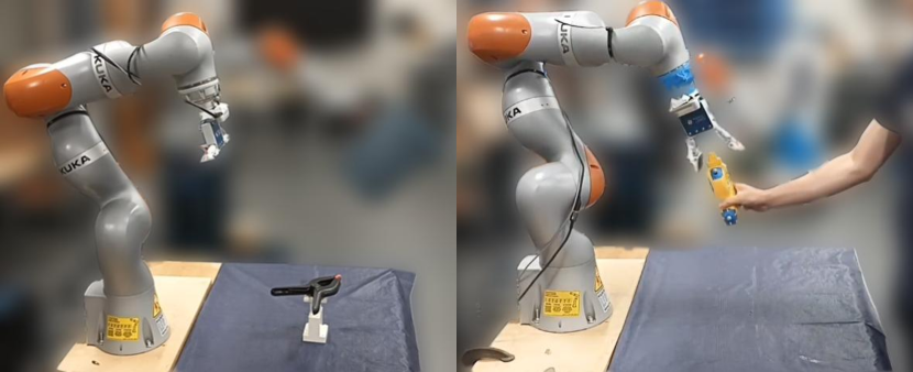
Figure 1: Robot experimental setup used to evaluate our feasible dynamic grasping framework (left: static object, right: dynamic object). An Intel RealSense camera mounted on the robot’s end-effector is used to obtain a partial point cloud of the object and its pose (optitrack is used to track the object in dynamic scenarios) with no prior knowledge about the object.

When addressing the robot’s kinematic constraints and collisions, two distinct approaches emerge: the explicit sampling of grasp poses achieved by learning kinematics and collisions implicitly [9], and the transformation of the grasp sampling challenge into a multi-objective optimization through the acquisition of a grasp pose cost or distance function [10, 11]. The former approach is computationally fast but restricted to the environmental setup and robot, hindering its applicability across diverse scenarios. In contrast, the latter approach is flexible and simple, as it can consider different constraints in the control optimization and not in the sampling steps. Moreover, it does not suffer from the challenges of grasp selection and can be applied to dynamic objects, unlike the linear bandit method [12] for static objects. However, extending this approach to task-specific grasp sampling, accounting for affordances, presents difficulties. Furthermore, SE(3) grasp pose distances don’t necessarily correlate with the nearest pose in joint space.

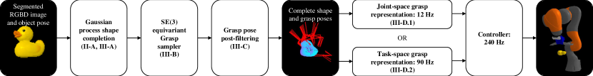
Figure 2: Feasible Dynamic Grasping Framework pipeline. Given a partial point cloud of an object and its pose, we reconstruct the shape using the Gaussian Process Distance Field (Section II-A) with a refined distance metric as in Section III-A. Next, we sample poses from an SE(3) equivariant grasp sampler (Section III-B). Finally, the discrete set of feasible grasp poses is used to i) construct a continuous Riemannian GMM for dynamic task-space control (Section III-D1) or ii) convert to joint-space via IK to construct a continuous GP for dynamic control in joint-space (Section III-D2).

In scenarios involving human-robot interaction (HRI), it is crucial to address dynamic objects and implement reactive control strategies [13]. One viable approach is to optimize the end-effector [14] or sampled trajectory [15] based on the object’s pose. Recent research has also explored leveraging the consistency of learned grasp latent vectors to match grasp poses across time steps [16, 17]. Furthermore, some use reinforcement learning for whole control policies for object handover scenarios [18]. These methods to learn the dynamics of grasping reduce the complexity of modeling different components related to grasping, but they are hard to directly apply to different scenes or methods.

Contribution In this work, we present a sequential modular approach designed to sample 6D grasp poses and perform reactive motion planning and control for dynamic objects (Figure 2). Our pipeline assumes we have a segmented point cloud of the object, which is assumed to be rigid. The proposed pipeline has three key steps:

1. Object Shape Reconstruction: We initiate by reconstructing the object’s shape using the Gaussian Process distance field [19]. This process yields an approximate signed distance field, which effectively measures the distance between the rigid object and points, which are in $\mathbb{R}^{3}$ Euclidean space, along with gradients. Such information enables the resampling of the object’s complete point cloud, offering a comprehensive representation.

2. SE(3) Equivariant Grasp Sampling and Filtering: Subsequently, our pipeline advances to SE(3) equivariant grasp sampling and filtering. By taking the complete point cloud as input, our data-driven grasp sampler generates SE(3) equivariant grasp samples. Employing Gaussian Mixture Model-based reachability analysis, we then conduct a post-filtering of sample grasp poses.

3. Grasp Pose Selection and Control: The third phase involves the selection of grasp poses and control, either within task space or joint space, as per the requirement. The pipeline utilizes either the Gaussian Mixture Model (GMM) of feasible grasp poses in task space or projects grasp poses into joint space, employing batched inverse kinematics and a Gaussian Process Distance Field (GPDF).

By seamlessly integrating these steps, our proposed pipeline offers an effective solution for generating and evaluating grasp poses while also facilitating motion planning and control within dynamic environments, see Figure 1.

II Preliminaries

Next we described the probabilistic and mathematical tools we use to build our feasible dynamic grasping framework.

II-A Gaussian Process Distance Field (GPDF)

Gentil et al. [19] introduced a novel approach for estimating an object’s distance field using Gaussian processes (GP) solely from its surface points. Given a point $\mathbf{x}\in\mathbb{R}^{m}$ and points $\mathbf{x}^{\prime}$ lying on the surface $\mathcal{S}\in\mathbb{R}^{m}$, the occupancy field $o(\mathbf{x})\in\mathbb{R}$ can be modeled as $o(\mathbf{x})\sim\mathcal{GP}(0,k_{o}(\mathbf{x},\mathbf{x}^{\prime}))$, where $k_{o}(d)$ represents the covariance kernel. The inferred occupancy from point $\mathbf{x}$ is calculated as follows:

$$\hat{o}(\mathbf{x})=k_{o}(\mathbf{x},\mathbf{X})(K_{o}(\mathbf{X},\mathbf{X})+\sigma_{o}^{2}I)^{-1}\mathbf{1}$$ (1)

By defining the inverse function $r$ as $r(k_{o}(\mathbf{x},\mathbf{x}^{\prime}))=||\mathbf{x}-\mathbf{x}^{\prime}||=d$, we can determine the distance field between $\mathbf{x}$ and the surface $\mathcal{S}$ as follows:

$$\hat{d}(\mathbf{x})=r(\hat{o}(\mathbf{x}))\$$ (2)

The gradient of the distance field, which can be used to obtain surface normals, can be analytically derived as:

$$\nabla d(\mathbf{x})=\frac{\partial r}{\partial o}\left(\nabla k_{o}(\mathbf{x},\mathbf{X})(K_{o}(\mathbf{X},\mathbf{X})+\sigma_{o}^{2}I)^{-1}\mathbf{1}\right)\$$ (3)

An advantageous characteristic of GP is their provision of an uncertainty measure, expressed as:

$$\mathbf{var}(o(\mathbf{x}))=k_{o}(\mathbf{x},\mathbf{x})$$ (4)

$$-k_{o}(\mathbf{x},\mathbf{X})(K_{o}(\mathbf{X},\mathbf{X})+\sigma_{o}^{2}I)^{-1}k_{o}(\mathbf{X},\mathbf{x})$$

This measure can be employed to assess the certainty of surface points. We use this GPDF to perform our shape completion step detailed in Section III-A.

II-B SE(3) equivariance

The SE(3) Lie group is well-used in robotics, particularly in describing end-effector and grasp poses. It offers a unified representation comprising rotation $R\in SO(3)$ and translation $t\in\mathbb{R}^{3}$. In this representation, a point is defined as $T=\big{[}\begin{smallmatrix}R&t\\ 0&1\end{smallmatrix}\big{]}\in SE(3)$. For grasp samplers focused on object-centric approaches [20, 21], SE(3) equivariance becomes a critical consideration. This requirement ensures that feasible grasp poses of an object remain consistent relative to the object’s pose. Consider a grasp sampler $f:\mathbb{R}^{3\times n}\rightarrow SE(3)$, where $\mathbf{P}\in\mathbb{R}^{3\times n}$ represents the object’s point cloud and $G=\big{[}\begin{smallmatrix}R_{G}&t_{G}\\ 0&1\end{smallmatrix}\big{]}\in SE(3)$ is a grasp pose. The condition for SE(3) equivariance is that $f(\mathbf{P})=G$ should satisfy

$$f(R\mathbf{P}+t)=RG+t$$ (5)

for any arbitrary rotation $R\in SO(3)$ and translation $t\in\mathbb{R}^{3}$. Many works achieve this by centering the point cloud $\mathbf{P}$ with it mean, $\frac{1}{n}\sum_{i}\mathbf{P}_{i}$, which gives translation-invariant input, and using a SO(3) equivariant neural network called Vector Neurons (VNN) [22]. Then, they re-center the output by adding the mean of the point cloud to the output. In this work, we employ the same approach to sample grasp poses, but using the grasp pose representation introduced by M. Sundermeye et al. [9], which is based on contact points.

II-C Gaussian Distribution on Riemannian manifold

In order to generate continuous distributions of SE(3) poses, which we require in both the grasp pose post-filtering stage (Section III-C) and the task-space reactive control formulation (Section III-D1). We leverage the Riemannian Expectation-Maximization (EM) algorithm proposed by S. Calinon [23], which is well-suited for Riemannian manifolds like SE(3) that have a left-invariant metric. Gaussian distribution in Riemannian manifold $\mathcal{M}$ is defined as

$$\mathcal{N}_{\mathcal{M}}(x|\mu,\Sigma)=((2\pi)^{d}|\Sigma|)^{-\frac{1}{2}}e^{-\frac{1}{2}\text{Log}_{\mu}(x)\Sigma^{-1}\text{Log}_{\mu}(x)}$$ (6)

In this equation, $\mu\in\mathcal{M}$ denotes the origin of the tangent space, $x\in\mathcal{M}$ represents a point on the manifold, $\Sigma\in\mathcal{T}\mu\mathcal{M}$ is a covariance defined in the tangent space of $\mu$, and $d$ corresponds to the dimension of the tangent space, which is 6 for SE(3). The mean of N points on the manifold, $\mu$, is iteratively computed as

$$u=\frac{1}{N}\sum_{i=1}^{N}\text{Log}_{\mu}(x_{i}),\quad\mu=\text{Exp}_{\mu}(u)$$ (7)

After convergence of $\mu$, the covariance is determined as

$$\Sigma=\frac{1}{N}\sum_{i=1}^{N}\text{Log}_{\mu}(x_{i})\text{Log}_{\mu}^{T}(x_{i})$$ (8)

One important consideration is that the logarithmic and exponential operations in the Riemannian manifold are different from those in the Lie group for SE(3). For example, $\text{Log}_{\mu}(x)$ is $[\text{Log}_{\mathcal{G}}(\mu^{-1}x)]^{\wedge}_{\mathcal{G}}$ for SE(3), where $\text{Log}_{\mathcal{G}}$ is a logarithmic operation of the Lie group and $[\quad]^{\wedge}_{\mathcal{G}}$ is an operation that changes the matrix to compact form in the Lie algebra.

III Method

Following we detail each step in our feasible dynamic grasping pipeline outline in Figure 2.

III-A Shape Completion with Distance Field Refinement

The Matern $\nu=1/2$ kernel, $k_{o}(d)=\sigma^{2}\exp\left(\frac{-d}{l}\right)$, with appropriate hyper-parameter settings ($l$ controlling interpolation degree, and $\sigma=1$) yields an approximate signed distance function (SDF) for the object. This outcome can be attributed to the well-known interpolation capabilities of GP, coupled with the fact that the inverse of the Matern $\nu=1/2$ kernel provides an analytical solution for $d$, which distinguishes it from other kernels that do not have analytic inverse solutions or yield non-bijective outputs such as $\sqrt{d^{2}}$. Nevertheless, its estimation accuracy deteriorates as it gets closer and inside the object, as in Figure 3 (left). To address this, we adopt an iterative refinement approach inspired by ray marching. This process operates under two fundamental assumptions: 1) The estimated distance field can be represented as a composite function, $d(\mathbf{x})=g(\text{SDF}(\mathbf{x}))$, where $g:\mathbb{R}\rightarrow\mathbb{R}$ is a monotonically increasing function that goes through the origin and SDF denotes the actual signed distance field; 2) The absolute value of the estimated distance field is less than or equal to the actual distance, meaning $|d(\mathbf{x})|\leq|\text{SDF}(\mathbf{x})|$. The iterative process involves projecting a point $\mathbf{x}$ onto the object’s surface using the equation:

$$\mathbf{x}\leftarrow\mathbf{x}-d(\mathbf{x})\frac{\nabla d(\mathbf{x})}{||\nabla d(\mathbf{x})||_{2}}$$ (9)

The accumulation of all $d(\mathbf{x})$ values throughout the iterations yields a refined estimate of the distance from the original $\mathbf{x}$. The normalized gradient of the distance field becomes the updated point’s surface normal. This is feasible due to the constant Eikonal function property of the signed distance function, which leads to the equation:

$$\frac{\nabla d(\mathbf{x})}{||\nabla d(\mathbf{x})||_{2}}=\frac{g^{\prime}\nabla\text{SDF}(\mathbf{x})}{||g^{\prime}\nabla\text{SDF}(\mathbf{x})||_{2}}$$ (10)

$$=\frac{g^{\prime}\nabla\text{SDF}(\mathbf{x})}{g^{\prime}||\nabla\text{SDF}(\mathbf{x})||_{2}}=\nabla\text{SDF}(\mathbf{x})$$

Therefore, provided the second condition is also met, the iterative process avoids overshooting and ultimately converges, as depicted on the right side of Figure 3. To determine the optimal parameter $l$ for GP, we employ the Acronym dataset [24] to create partial point clouds for 8872 objects. For each $l$ value, we construct a GPDF and compute the mean distance between the complete point cloud of the object and the GP-derived surface—similar to the Chamfer distance metric. A small $l$ yields a large mean distance, indicating poor reconstruction of the unseen object portions. Conversely, an excessively large $l$ leads to over-interpolated object shapes, resulting in a loss of high-curvature details. While adaptive $l$ selection based on the object’s point cloud size is feasible, we fix it at $l=0.3m$ based on grid search of $l=[0,0.6]$. This process facilitates obtaining a rough object shape, as demonstrated in Figure 4.

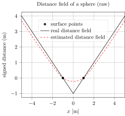
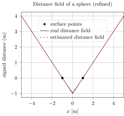
Figure 3: A 1D slice of a distance field of a sphere point cloud. The image on the left illustrates a comparison between the ground truth SDF and the initial estimation derived from the GPDF. On the right, the image illustrates an improved estimation achieved through five iterations of gradient descent, employing the ray marching concept.

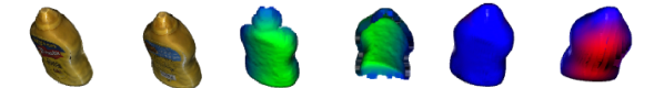
Figure 4: The reconstructed result using the Gaussian Process. The initial two images on the left display the mesh representation of a mustard bottle. In the subsequent two images, partial point clouds of the object are displayed. Finally, the last set of images shows the reconstructed point cloud of the object. In this representation, areas with low shape uncertainty are colored blue, while regions with high shape uncertainty are highlighted in red.

III-B Data-driven grasp sampler

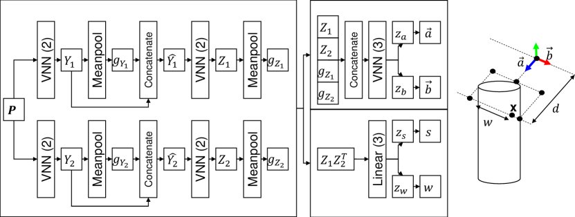
Figure 5: The architecture of the data-driven grasp sampler, with the numbers (*) denoting the respective number of layers in each component.

We use two VNN PointNet encoders and one VNN decoder for SO(3) equivariant features and one linear decoder for SO(3) invariant features, as in Figure 5. The input to our network, denoted as $\mathbf{P}\in\mathbb{R}^{n\times 2\times 3}$, encompasses both surface points $\mathbf{x}_{s}\in\mathbb{R}^{n\times 3}$ and their surface normals $\nabla d(\mathbf{x}_{s})\in\mathbb{R}^{n\times 3}$ extracted from GP. The generation of surface points is executed through the creation of an 8x8x8 grid within the expanded bounding box of the partial point cloud, centered around its midpoint. It’s important to note that this configuration might be adapted according to the camera’s orientation. The network’s primary objective is twofold: first, to determine whether a given point in $\mathbf{x}_{s}$ is a potential contact point on one side of the gripper; second, if viable, to estimate two columns of the rotation matrix and the width between the contact points. To validate if this grasp pose estimation is feasible, we get points on the gripper, transform points based on the grasp pose, and then input them into GP to verify whether they lie outside the object’s surface. Once we ascertain that all points are indeed situated outside the object, we proceed to retrieve the surface normals of the paired contact points $\mathbf{x}$ and $\mathbf{x}^{\prime}=\mathbf{x}-w\vec{b}$ from GP. Subsequently, we examine whether the cosine similarity between the surface normals of these contact pairs closely approximates -1. This similarity metric serves as an indicative measure of force closure for jaw grippers.

III-C Reachable-Space Riemannian Mixture Model (RMM)

Reachability serves as a metric through which a robot manipulator determines the feasibility of reaching a desired workspace pose $G\in SE(3)$ using a specific joint configuration $q\in\mathbb{R}^{n}$. Reachability has been used for mobile manipulators as an indication that the leg or wheels of the robot have to move [25, 26] or for fixed manipulators to optimize grasp poses [14, 15] from the robot’s kinematic perspective. We are inspired by the work of Kim et al. [14], who employed a GMM to pre-learn reachability. This was accomplished by utilizing end-effector samples from a dataset of joint configurations, thereby enabling the optimization of end-effector poses in conjunction with grasp pose GMM. They fitted GMM by flattening out the first two columns of the rotation matrix and translation, which gave better results than using Euler angles or quaternions.

In this work, we instead learn the reachable space based on the Riemannian Gaussian distribution introduced in Section II-C. To construct an offline reachable-space Riemannian Gaussian Mixture Model (RMM), we utilize end-effector poses derived from forward kinematics. From a pool of $10^{7}$ joint configurations, we perform downsampling, retaining approximately $3\times 10^{6}$ samples. We exclude self-collision samples and samples below 0.1 m since the robot is on the table. This will prevent the selection of grasp poses that cause collisions with the table. We can also prevent collisions by fitting another GPDF for the environment with a larger $l$ parameter. However, in our experiment, we assume a simple environment that is not heavily clustered, which requires less additional GP. To select the number of clusters, we used the Bayesian information criterion (BIC) and chose 64 clusters from a range of $k=[1,70]$. We use K-means++ for initialization and a probability threshold encompassing 99% of the dataset points. When a pose’s probability falls below the threshold, it is regarded as an unreachable.

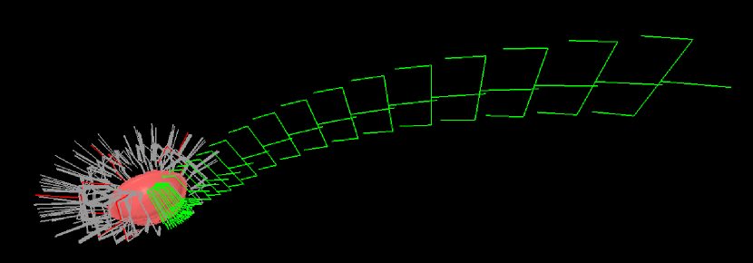
Figure 6: The gray grasp poses represent the outputs from the grasp sampler, while the four red grasp poses correspond to clusters’ means identified by the GMM. The green trajectory of the end-effector illustrates a gradient ascent outcome, converging towards a feasible point.

III-D Continuous Grasp Pose Distributions for Control

After filtering the grasp poses using our proposed reachable-space, it’s possible that multiple viable grasp poses remain. Due to the discrete nature of these samples, establishing a stable gradient for control, particularly in the presence of disturbances, becomes challenging. Therefore, we propose two strategies to make the distribution of grasp poses continuous: a task-space grasp representation using RMM, and a joint-space grasp representation using GPDF. Using these, we move away from discrete grasp selection and instead utilize existing motion planning algorithms to navigate around collisions for dynamic objects.

III-D1 Task-Space Grasp Distribution

RMM is fitted to the sample grasp poses, assigning higher probabilities to more plausible poses. This enables the computation of the gradient of the robot’s end-effector pose through gradient ascent on the RMM and differential inverse kinematics. When dealing with a RMM for SE(3), the probability of the pose $x$ is expressed as:

$$\mathcal{P}(x|\mu,\Sigma)=\sum_{i=1}^{n}\pi_{i}\mathcal{N}_{\mathcal{M}}(x|\mu_{i},\Sigma_{i})$$ (11)

where $n$ is the number of clusters, and $\pi_{i}$, $\mu_{i}$, and $\Sigma_{i}$ denote the weight, mean, and covariance of the $i$th cluster. the gradient can be computed as follows, with $\theta_{*}=\{\mu_{*},\Sigma_{*}\}$:

$$\frac{\partial\mathcal{P}(x|\theta)}{\partial x}= \sum_{i=1}^{n}\pi_{i}\mathcal{N}_{\mathcal{M}}(x|\theta_{i})J_{r}^{-1}(\mu^{-1})(-\Sigma^{-1}\text{Log}_{\mu_{i}}(x))$$ (12)

$J_{r}$ represents the right Jacobian of SE(3) [27]. Since obtaining $J_{r}$ analytically can be challenging, we rely on numerical methods for gradient computation. Subsequently, we use $\frac{\partial\mathcal{P}(x|\theta)}{\partial x}$ to derive the joint-space velocity controller,

$$\dot{q}=J(q)^{\dagger}\frac{\partial\mathcal{P}(x|\theta)}{\partial x}$$ (13)

where $J(q)$ is the manipulator Jacobian and ^† the Pseudo-Inverse. Eq. 13 acts as gradient ascent to the closest grasp pose (local maxima of GMM) from the robot’s current pose (Figure 6). However, there are two problems with using raw GMM gradients: zero gradient in local minima and zero gradient for poses distant from grasp poses. To escape from the local minima, we sample surrounding points and add a disturbance if they are identified as local minima. To solve the second problem, we use log probability instead,

This gradient has a numerical advantage when the probability is very low since multiplying the constant value to the probability $\mathcal{N}_{\mathcal{M}}(x|\theta_{i})$ for all $i$ gives the same results. For dynamic objects, we transform the means along with the object and get the gradient. To consider reachability we transform the means and refit with the reachable grasp poses.

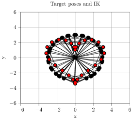
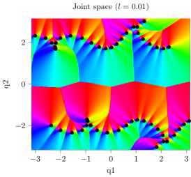
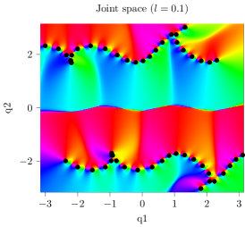
Figure 7: Joint-space gradient field derived from GPDF using a 2D robot’s IK solutions. The graph on the left displays end-effector targets as red points, accompanied by their respective IK solutions. The middle and right graphs display the joint-space gradient with varying interpolation value $l$.

III-D2 Joint-Space Grasp Distribution

Alternatively, if we have an inverse kinematics (IK) solver for a $n$-DoF robot with joint limits that can yield diverse solutions of $q\in\mathbb{R}^{n}$ for a set of end-effector poses, we can create a $n$-D distance field using GPDF on the IK solutions. As GPDF is a monotonically increasing function it can be considered a potential function with multiple equilibria. We thus propose the following joint-space velocity controller,

$$\dot{q}=-d_{q}(q)\nabla d_{q}(q),$$ (15)

obtained from the GPDF fitted on the IK solutions, $d_{q}$, as shown in Figure 7 for 2-DoF example. However, sampling multiple IK solutions in short period of time is not easy. Therefore, we use the combination of the learning-based method, IKFlow [28], and the batched-damped pseudo-inverse method with batched forward kinematics and Jacobian calculation [29]. IKFlow gives multiple IK solutions that already consider self-collision and joint limits at almost 100 Hz using normalizing flow. However, its solutions tend to lack accuracy compared to the pseudo-inverse method. Therefore, we first sample IK solutions with IKFlow and refine them with the pseudo-inverse method for 3 iterations. To fit GP, we use solutions that only satisfy the maximum error threshold. For dynamic objects, we transform grasp poses based on the object pose and re-sample IK solutions with the same seed for IKFlow, which leads to solutions that smoothly change from the previous solutions. For reachability, we disregard grasp poses that are unreachable.

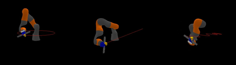
Figure 8: Dynamic object trajectories in sim. (circular, linear, sinusoidal).

IV Experiments

IV-A Experimental Setup

Our experimental setup involves a KUKA iiwa 7 manipulator equipped with a SAKE gripper and a Realsense D435 depth camera, which we employ for both real robot and simulation experiments. Both task and joint space grasp representation run in the Intel i7-11700K without GPU. Our primary objectives are twofold: firstly, to assess the quality of grasp poses generated by the grasp sampler pipeline, and secondly, to evaluate the feasibility of dynamic object grasping using joint and task space grasp representations.

IV-A1 Grasp Sampler Test

To evaluate grasp poses, we conduct experiments in both simulation and on a real robot, assuming that the object remains static. In both scenarios, we utilize the YCB datasets [30], which were not part of the training dataset for the data-driven grasp sampler. The dataset is scaled if the object is too big for the SAKE gripper. In the simulation environment, we employ Pybullet with fine-tuned friction coefficients and test with 50 different YCB objects. The object begins at a random pose within a 10cm cube located at (x: 40cm, y: 0cm, z: 60cm) in the robot’s base coordinate, and the robot follows these steps: capturing a segmented RGBD image of the object, sampling grasp poses, filtering these poses, employing task-space grasp representation to attain a stable pose, grasping the object, applying gravity, and finally moving into a lifting pose. The success criterion in this case is determined by whether the object remains stable for at least 2 seconds after the robot transitions to the lifting pose. And we do this 10 times for each object. For the real robot experiment (Figure 1), we provide a segmented RGBD image to the robot using the method described in [31], sample grasp poses, convert them to joint space grasp representations, and assess the robot’s ability to successfully grasp the objects.

TABLE I: Grasp success rate for static object in simulation

Method	Accuracy (%)
Grasp sampler	77.60 (24.54)
Grasp sampler + Post-filtering	88.60 (15.75)
Grasp sampler + Post-filtering + Reachability analysis	90.00 (11.49)

TABLE II: Comparison between task and joint space methods during dynamic object grasping in simulation

Trajectory	Grasp representation	Self collision (%)	Joint limit violations (%)	Manipulability	Gripper frame distance to object frame (cm)
Circular	Joint space	1.08 (0.57)	57.06 (6.52)	0.0936 (0.0017)	16.65 (0.96)
	Task space	6.72 (5.55)	89.64 (0.74)	0.0729 (0.0022)	3.31 (0.25)
Linear	Joint space	0.00 (0.00)	55.49 (5.34)	0.0887 (0.0052)	6.44 (0.24)
	Task space	3.84 (2.12)	62.90 (30.58)	0.0785 (0.0076)	2.70 (0.19)
Sinusoidal	Joint space	0.00 (0.00)	55.64 (3.82)	0.0884 (0.0021)	12.47 (0.45)
	Task space	1.03 (1.97)	91.63 (5.63)	0.0847 (0.0033)	7.10 (0.77)

IV-A2 Dynamic Object Test

To determine the robot’s capability to reach appropriate grasp poses for a dynamically moving object in simulation, we generate three types of trajectories: circular, linear, and sinusoidal, each featuring a constant rotation of the object as in Figure 8. Then, we test five times for each trajectory and see the robot’s joint limit violation, manipulability, and self-collision without constraints. We define manipulability as $m=\sqrt{\det(J(q)J(q)^{T})}$. In real-world testing (Figure 1), we segment the RGBD image of the object, track its movement (going left and right of the robot) using a calibrated Optitrack tracking system relative to the robot’s base frame, and control the robot based on sampled grasp poses and check its grasp success.

IV-B Experimental Results and Discussion

IV-B1 Grasp quality

In simulation, the success rate of grasping is 90.00% for a total of 500 trials with 50 different YCB objects, as in Table I. Without post-filtering, the grasp success rate drops significantly. This emphasizes the importance of validating sampled grasp poses. Our data-driven grasp sampler is a small model that runs within 10 ms for a point cloud size of 1024 points in CPU. Therefore, some samples that grasp sampler outputs are inaccurate. Having full shape information from the distance field helps to accommodate those errors. The limitation of this is that the result might become so conservative that it only gives a few possible grasp poses. For those cases, we can consider the similar approach we took with IKFlow, where we sample IK solutions from a data-driven method and use a numerical method to refine those, such that we run grasp pose optimization [2] using initial samples from a data-driven grasp sampler. The reachability analysis only added marginal accuracy to the grasp sampler as the objects were already near the robot, where most grasp poses are reachable. Post-filtering and reachability analysis can be done in less than 5 ms. However, since GP has complexity of $O(n^{3})$ where $n$ is the number of point clouds, GP becomes a bottleneck for the grasp sampling process. For 512 points, it takes around 0.25 seconds, and for 1024 points, it takes between 1-2 seconds.

For real robot testing with static objects, 14/16 grasps were successful for 8 different objects. The failures happened with the drill due to its heavy unbalanced weights on the head and the banana due to the slip caused by too strong grasp. Since we are only considering the shape of the object, this errors happen even though initial grasp contacts are good. For eight dynamic objects, 19/24 grasps were successful. The failures happened again with the same reasons as static cases.

TABLE III: Frequency of task and joint space methods

Number of GMM means	1	2	3	4	5	6	7	8	9	10
Frequency (Hz)	106.6	99.4	95.7	90.2	88.6	85.2	83.1	81.1	79.4	78.2
Number of GP’s samples	10	20	30	40	50	60	70	80	90	100
Frequency (Hz)	22.4	18.3	16.7	17.2	16	15.1	15.8	14.8	14.1	13.9

IV-B2 Comparison between task and joint space methods

The task space method outperforms the joint space method in terms of computational efficiency, as evidenced in Table III. Specifically, the task space method exhibits significantly faster execution times, making it a more attractive choice. It is important to note that the frequency of the task space method exhibits a nearly linear decrease with an increasing number of GMM means, typically requiring only 4 to 8 means to adequately represent object grasp poses. In contrast, the frequency of the joint space method does not exhibit a straightforward linear relationship with the number of IK solutions, largely due to the advantages of parallel computing.

Interestingly, the joint space method can exhibit speed improvements even as the number of samples increases, due to parallel computations and memory allocations at every power of 2. However, it’s crucial to highlight that achieving smooth control with the joint space method necessitates a substantial number of samples, typically approaching 100, to ensure that joint poses change gradually and avoid sudden transitions. From a robot kinematics perspective, the joint space method demonstrates superior performance over the task space method, as indicated in Table II. This superiority stems from the task space method’s susceptibility to getting stuck in positions where singularities occur, while the joint space method possesses the capability to navigate around singularities, joint limits, and self collision. Consequently, the joint space method achieves higher manipulability scores compared to the task space method.

While it may seem that the joint space method could outperform the task space method solely by achieving higher speeds, this assumption oversimplifies the comparison. For example, in a HRI scenario like object handovers, the joint-space method is less legible for the human and hence can seem inefficient, as shown in the average distance between the gripper frame and the object frame. Distance tends to increase for the joint space method as it makes big motions when it tries to escape from singularities or joint limits. In our real robot object handover testing, the task space method was preferable in that respect. The suitability of each method depends on the requirements and constraints of the task.

V CONCLUSION

In conclusion, our research focuses on making robots better at grabbing objects in dynamic situations. We emphasize the importance of considering the object’s shape, possible collisions, and how the robot moves when designing a good grasping strategy. We introduced a step-by-step approach that uses Gaussian Process Distance Field for object shape reconstruction, SE(3) equivariant grasp sampling and filtering, and Riemannian Mixture Models for grasp pose selection and control, to help robots grasp more effectively. The proposed method offers a feasible solution for generating and evaluating grasp poses, as well as facilitating motion planning and control in dynamic environments.

References

- [1] V.-D. Nguyen, “Constructing force-closure grasps,” The International Journal of Robotics Research, vol. 7, no. 3, pp. 3–16, 1988.
- [2] D. Turpin, T. P. Zhong, S. Zhang, G. Zhu, J. Liu, E. Heiden, M. Macklin, S. Tsogkas, S. Dickinson, and A. Garg, “Fast-grasp’d: Dexterous multi-finger grasp generation through differentiable simulation,” 2023 IEEE International Conference on Robotics and Automation (ICRA), pp. 8082–8089, 2023.
- [3] Y. Wu, W. Liu, Z. Liu, and G. S. Chirikjian, “Learning-free grasping of unknown objects using hidden superquadrics,” ArXiv, vol. abs/2305.06591, 2023.
- [4] S.-H. Kim, T. Ahn, Y. Lee, J. Kim, M. Y. Wang, and F. C. Park, “Dsqnet: A deformable model-based supervised learning algorithm for grasping unknown occluded objects,” IEEE Transactions on Automation Science and Engineering, vol. 20, pp. 1721–1734, 2023.
- [5] Y. Lin, C. Tang, F.-J. Chu, and P. A. Vela, “Using synthetic data and deep networks to recognize primitive shapes for object grasping,” 2020 IEEE International Conference on Robotics and Automation (ICRA), pp. 10494–10501, 2019.
- [6] J. Varley, C. DeChant, A. Richardson, J. Ruales, and P. K. Allen, “Shape completion enabled robotic grasping,” 2017 IEEE/RSJ International Conference on Intelligent Robots and Systems (IROS), pp. 2442–2447, 2016.
- [7] A. Mousavian, C. Eppner, and D. Fox, “6-dof graspnet: Variational grasp generation for object manipulation,” 2019 IEEE/CVF International Conference on Computer Vision (ICCV), pp. 2901–2910, 2019.
- [8] M. V. der Merwe, Q. Lu, B. Sundaralingam, M. Matak, and T. Hermans, “Learning continuous 3d reconstructions for geometrically aware grasping,” 2020 IEEE International Conference on Robotics and Automation (ICRA), pp. 11516–11522, 2019.
- [9] M. Sundermeyer, A. Mousavian, R. Triebel, and D. Fox, “Contact-graspnet: Efficient 6-dof grasp generation in cluttered scenes,” 2021 IEEE International Conference on Robotics and Automation (ICRA), pp. 13438–13444, 2021.
- [10] T. Weng, D. Held, F. Meier, and M. Mukadam, “Neural grasp distance fields for robot manipulation,” 2023 IEEE International Conference on Robotics and Automation (ICRA), pp. 1814–1821, 2022.
- [11] J. Urain, N. Funk, J. Peters, and G. Chalvatzaki, “Se(3)-diffusionfields: Learning smooth cost functions for joint grasp and motion optimization through diffusion,” 2023 IEEE International Conference on Robotics and Automation (ICRA), pp. 5923–5930, 2022.
- [12] L. Wang, Y. Xiang, and D. Fox, “Manipulation trajectory optimization with online grasp synthesis and selection,” ArXiv, vol. abs/1911.10280, 2019.
- [13] A. Billard, S. S. Mirrazavi Salehian, and N. Figueroa, Learning for Adaptive and Reactive Robot Control: A Dynamical Systems Approach. Cambridge, USA: MIT Press, 2022.
- [14] S. Kim, A. Shukla, and A. Billard, “Catching objects in flight,” IEEE Transactions on Robotics, vol. 30, pp. 1049–1065, 2014.
- [15] I. Akinola, J. Xu, S. Song, and P. K. Allen, “Dynamic grasping with reachability and motion awareness,” 2021 IEEE/RSJ International Conference on Intelligent Robots and Systems (IROS), pp. 9422–9429, 2021.
- [16] J. Liu, R. Zhang, H. Fang, M. Gou, H. Fang, C. Wang, S. Xu, H. Yan, and C. Lu, “Target-referenced reactive grasping for dynamic objects,” 2023 IEEE/CVF Conference on Computer Vision and Pattern Recognition (CVPR), pp. 8824–8833, 2023.
- [17] H. Fang, C. Wang, H. Fang, M. Gou, J. Liu, H. Yan, W. Liu, Y. Xie, and C. Lu, “Anygrasp: Robust and efficient grasp perception in spatial and temporal domains,” ArXiv, vol. abs/2212.08333, 2022.
- [18] S. Christen, W. Yang, C. P’erez-D’Arpino, O. Hilliges, D. Fox, and Y.-W. Chao, “Learning human-to-robot handovers from point clouds,” 2023 IEEE/CVF Conference on Computer Vision and Pattern Recognition (CVPR), pp. 9654–9664, 2023.
- [19] C. L. Gentil, O.-L. Ouabi, L. Wu, C. Pradalier, and T. Vidal-Calleja, “Accurate gaussian process distance fields with applications to echolocation and mapping,” ArXiv, vol. abs/2302.13005, 2023.
- [20] A. Simeonov, Y. Du, A. Tagliasacchi, J. B. Tenenbaum, A. Rodriguez, P. Agrawal, and V. Sitzmann, “Neural descriptor fields: Se(3)-equivariant object representations for manipulation,” 2022 International Conference on Robotics and Automation (ICRA), pp. 6394–6400, 2021.
- [21] B. Sen, A. Agarwal, G. Singh, B. Brojeshwar, S. Sridhar, and M. Krishna, “Scarp: 3d shape completion in arbitrary poses for improved grasping,” 2023 IEEE International Conference on Robotics and Automation (ICRA), pp. 3838–3845, 2023.
- [22] C. Deng, O. Litany, Y. Duan, A. Poulenard, A. Tagliasacchi, and L. J. Guibas, “Vector neurons: A general framework for so(3)-equivariant networks,” 2021 IEEE/CVF International Conference on Computer Vision (ICCV), pp. 12180–12189, 2021.
- [23] S. Calinon, “Gaussians on riemannian manifolds: Applications for robot learning and adaptive control,” IEEE Robotics & Automation Magazine, vol. 27, pp. 33–45, 2019.
- [24] C. Eppner, A. Mousavian, and D. Fox, “Acronym: A large-scale grasp dataset based on simulation,” 2021 IEEE International Conference on Robotics and Automation (ICRA), pp. 6222–6227, 2020.
- [25] S. Jauhri, J. Peters, and G. Chalvatzaki, “Robot learning of mobile manipulation with reachability behavior priors,” IEEE Robotics and Automation Letters, vol. 7, pp. 8399–8406, 2022.
- [26] N. Vahrenkamp, T. Asfour, and R. Dillmann, “Robot placement based on reachability inversion,” 2013 IEEE International Conference on Robotics and Automation, pp. 1970–1975, 2013.
- [27] G. S. Chirikjian, “Stochastic models, information theory, and lie groups, volume 2,” 2012.
- [28] B. Ames, J. Morgan, and G. D. Konidaris, “Ikflow: Generating diverse inverse kinematics solutions,” IEEE Robotics and Automation Letters, vol. 7, pp. 7177–7184, 2021.
- [29] S. Zhong, T. Power, and A. Gupta, “PyTorch Kinematics,” 3 2023.
- [30] B. Çalli, A. Walsman, A. Singh, S. S. Srinivasa, P. Abbeel, and A. M. Dollar, “Benchmarking in manipulation research: The ycb object and model set and benchmarking protocols,” ArXiv, vol. abs/1502.03143, 2015.
- [31] C. Zhang, D. Han, Y. Qiao, J. U. Kim, S.-H. Bae, S. Lee, and C. S. Hong, “Faster segment anything: Towards lightweight sam for mobile applications,” arXiv preprint arXiv:2306.14289, 2023.