Jet mixing enhancement with Bayesian optimization, deep learning, and persistent data topology

Abstract

We optimize the jet mixing using large eddy simulations (LES) at a Reynolds number of 3000. Key methodological enablers consist of Bayesian optimization, a surrogate model enhanced by deep learning, and persistent data topology for physical interpretation. The mixing performance is characterized by an equivalent jet radius ($R_{\rm eq}$) derived from the streamwise velocity in a plane located 8 diameters downstream. The optimization is performed in a 22-dimensional actuation space that comprises most known excitations. This search space parameterizes distributed actuation imposed on the bulk flow and at the periphery of the nozzle in the streamwise and radial directions. The momentum flux measures the energy input of the actuation. The optimization quadruples the jet radius $R_{\rm eq}$ with a $7$-armed blooming jet after around $570$ evaluations. The control input requires $2\%$ momentum flux of the main flow, which is one order of magnitude lower than most ad hoc dual-mode excitations. Intriguingly, a pronounced suboptimum in the search space is associated with a double-helix jet, a new flow pattern. This jet pattern results in a mixing improvement comparable to the blooming jet. A state-of-the-art Bayesian optimization converges towards this double helix solution. The learning is accelerated and converges to another better optimum by including surrogate model trained along the optimization. Persistent data topology extracts the global and many local minima in the actuation space and can be identified with flow patterns beneficial to the mixing.

1 Introduction

Jet flows are ubiquitous in nature and technology and belong to a handful of configurations described in any fluid mechanics textbook. Jet mixing plays a pivotal role in many engineering applications, e.g. fuel injection in engines, combustor cooling, chemical mixing, printing, and noise generation (Jordan & Colonius, 2013), just to name a few. Hence, jet mixing optimization plays an important part in academic research and engineering applications.

Laminar jets are affected by the Kelvin-Helmholtz instability of the initial shear layer (Ball et al., 2012). The jet shear layer rolls up into pronounced vortex rings. Excitation at the nozzle exit provides authority over the vortex formation, e.g. allows to speed up the vortex formation, to support or mitigate vortex pairing, and to influence the far-field coherent structures. Vortex pairing in streamwise direction promotes larger mixing regions observed as the orderly ‘vortical puffs’ with axisymmetric excitation (Crow & Champagne, 1971). More importantly, a significant increase in the spreading angle can be obtained by vortex splitting evolving along several branches (Lee & Reynolds, 1985).

The actuation may promote axisymmetric, helical, dual-mode, flapping, and bifurcating dynamics. In particular, acoustic excitation of bulk affects the jet spreading via controlled vortex pairing (Crow & Champagne, 1971; Hussain & Zaman, 1980). Jet mixing is more effectively augmented with helical forcing (Mankbadi & Liu, 1981; Corke & Kusek, 1993). Bifurcating, trifurcating, and blooming jets appear with a spreading angle up to $80^{\circ}$ when axisymmetric and helical modes are combined (dual-mode) with different frequency ratios (Lee & Reynolds, 1985). The flapping mode is composed of counter-rotating helical modes, and the combination of axisymmetric and flapping modes is referred to as bifurcating mode. Both the flapping and the bifurcating mode can produce bifurcating jets with an impressive jet spreading (Parekh, 1989; Danaila & Boersma, 2000; da Silva & Métais, 2002).

The world of multiple-mode actuation for mixing optimization holds considerable promise and is still to be explored. The radial excitation with three flapping modes including $9$ parameters is optimized by Evolution Strategies (Koumoutsakos et al., 2001). Only one dominant flapping mode remains after $400$ Direct Numerical Simulations (DNS) at $Re=500$. In the sequel, the bifurcating mode using axial forcing is optimized for $Re$ up to $1500$ using the amplitudes and two Strouhal numbers as control parameters (Hilgers & Boersma, 2001). In an adjoint-based optimization study at $Re=2000$, radial forcing is found more effective than axial actuation in the dual-mode forcing (Shaabani-Ardali et al., 2020). In an experiment at $Re=8000$, jet mixing is manipulated with periodic operation of six radial minijets. In 200 evaluations, Bayesian optimization minimizes a streamwise centerline velocity tuning 12 parameters, the frequency, amplitudes and phase differences (Blanchard et al., 2021). The optimal mixing is facilitated by combining flapping and helical forcing, like machine learning control for the same configuration (Zhou et al., 2020).

Evidently, the flow control performance should benefit from the deployment of more actuators and richer actuation space. In this spirit, an intelligent nozzle with eighteen electromagnetic flap actuators (Suzuki et al., 1999), and localized arc filament plasma actuators (LAFPAs) (Utkin et al., 2006) have been developed for jet control. Bayesian Optimisation (BO) holds the promise of effectively conquering of the high-dimensional search space (Blanchard et al., 2021). BO is designed to optimize black-box functions that are costly to evaluate and can incorporate prior assumptions about the cost function (Shahriari et al., 2015). BO sequentially derives the next actuation to evaluate given by a surrogate model trained on all the queried data. The two key issues in BO are the choice of sequential strategy (Blanchard & Sapsis, 2021) and the surrogate model. Recently, the deep operator network (DeepONet) with a small generalization error is proposed (Lu et al., 2021) and applied as the surrogate model to improve the extreme event forecast (Pickering et al., 2022). Different from the well-known Gaussian process (GP) which parameterizes the input, DeepONet can map input time-dependent functions to the output.

The present study builds on a jet mixing plant employing Large Eddy Simulations (LES) and a rich streamwise and radial actuation space at the nozzle exit. This plant can reproduce virtually all previously considered actuated jet dynamics as elements of a high-dimensional search space. High-dimensional optimization constitutes a challenge that is tackled by a Bayesian optimizer enhanced by deep learning using DeepONet.

The paper is organized as follows. The configuration, actuation, metrics, and optimizer are defined in §2. The learning process and the optimized solutions are discussed in §3. The findings and the outlook are summarized in §4.

2 Setup and methods

2.1 Jet configuration

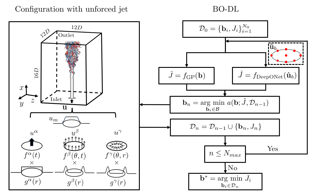
Figure 1: Problem setup including the jet configuration with the designed actuation (left) and the deep learning enhanced Bayesian optimization (right). $\mathbf{b}$ is the actuation parameter. $\hat{\mathbf{u}}_{b}$ is the actuation command at the 9 red points indicated in the dashed box.

The configuration is a jet flow exiting a circular nozzle of diameter $D$ in Fig. 1. The flow is described in a Cartesian coordinate system $(x,y,z)$ where $x$ represents the streamwise direction and the origin coincides with the center of the nozzle. The computational domain starts from the exit and covers a rectangular region with size $12D\times 16D\times 12D$. The main flow features are captured with a small influence of the side boundaries. The actuation $\bm{u}_{b}(r,\theta,t)$ is imposed with the mean streamwise velocity $u_{m}(r)$ as the inlet velocity profile $u(r,t)$,

$$\bm{u}(r,t)=u_{m}(r)\bm{e}_{x}+\bm{u}_{b}(r,\theta,t),$$

where $r$ measures the radial distance from the centerline, and $\theta$ is the azimuthal angle. The mean streamwise component has a hyperbolic-tangent profile,

$$u_{m}(r)=\frac{u_{j}+u_{c}}{2}-\frac{u_{j}-u_{c}}{2}\tanh\left(\frac{1}{4}\frac{R}{\delta_{2}}\left(\frac{r}{R}-\frac{R}{r}\right)\right),$$

where $u_{j}$ is the jet centerline velocity, $u_{c}=0.03u_{j}$ is the co-flow velocity to mimic a natural suction process, and $\delta_{2}=R/20$ is the momentum boundary layer thickness of the initial shear layer. The actuation term $\bm{u}_{b}$ is described in §2.2. The side and outlet boundary conditions are detailed in Tyliszczak (2014, 2018).

The simulations are conducted with an in-house high-order LES solver (Tyliszczak, 2014), which has been verified and validated in the studies of natural and excited jets (Tyliszczak, 2018; Boguslawski et al., 2019), with similar dynamic scales as the present work.

The low Reynolds number $\Rey=u_{j}D/\nu=3000$, $\nu$ representing the kinematic viscosity, allows the use of a relatively coarse computational mesh to obtain a reliable large LES database at a reasonable computation cost. Two meshes are employed in this study. A coarse mesh with $80\times 160\times 80$ nodes is used for the learning process and a refined mesh with $192\times 336\times 192$ nodes for the validation and flow analysis of selected cases. A single simulation on the coarse mesh takes half an hour with $40$ processors and the whole optimization process with $1000$ converged simulations lasts for around $21$ days.

2.2 General axial and radial actuation

We define the actuation $\bm{u}_{b}$ with a general expression, without assumption on the forcing mode. The term $\bm{u}_{b}$ includes an axisymmetric streamwise bulk forcing $u^{\alpha}(r,\theta,t)$, and a peripheral forcing with the streamwise component $u^{\beta}(r,\theta,t)$, and the radial $u^{\gamma}(r,\theta,t)$:

$$\bm{u}_{b}=\left(u^{\alpha}+u^{\beta}\right)\bm{e}_{x}+u^{\gamma}\bm{e}_{r}.$$ (1)

The forcing components are the product of a perturbation $f^{m}(\theta,t)$ and a radial profile $g^{m}(r)$: $u^{m}(r,\theta,t)=f^{m}(\theta,t)g^{m}(r)$, $m=\alpha,\beta,\gamma$ with $g^{\alpha}(r)=1$ for $r\leq R$ and $0$ for $r>R$, and $g^{\beta}(r)=g^{\gamma}(r)=\exp(-1000(R-r)^{2.5})$. The profiles of the three forcing components are depicted in Fig. 1. The perturbation terms $f^{m}(\theta,t)$ are defined as the sum and product of space- and time-harmonic functions:

$$f^{\alpha}(t) = \sum_{i=-L}^{L}\alpha_{i}\>\Theta_{i}(\omega_{\alpha}t)$$ (2)

$$f^{\beta}(\theta,t) = \sum_{i,j=-L,\ldots,L}\beta_{ij}\>\Theta_{i}(\theta)\>\Theta_{j}(\omega_{\beta}t)$$ (3)

$$f^{\gamma}(\theta,t) = \sum_{i,j=-L,\ldots,L}\gamma_{ij}\>\Theta_{i}(\theta)\>\Theta_{j}(\omega_{\gamma}t),$$ (4)

where $\alpha_{i}$, $\beta_{ij}$, $\gamma_{ij}$ and $\omega_{\alpha}$, $\omega_{\beta}$, $\omega_{\gamma}$ are the actuation amplitudes and angular frequencies, respectively. $\Theta_{i}(\phi)$ is the harmonic function basis defined as: $\Theta_{i}(\phi)=\sin(i\phi)$ for $i>0$, $\Theta_{i}(\phi)=1$ for $i=0$, and $\Theta_{i}(\phi)=\cos(i\phi)$ for $i<0$. In this study, focus is placed on the first order expansion ($L=1$) of (2-4). Thus, the control law is parameterized by a $22$-dimensional vector $\mathbf{b}$,

$$\mathbf{b}=\left[St_{\alpha},St_{\beta},St_{\gamma},\alpha_{1},\left\{\beta_{ij}\right\}_{i,j=-1,0,-1},\left\{\gamma_{ij}\right\}_{i,j=-1,0,-1}\right]^{\intercal}\in\mathcal{B},$$ (5)

where the Strouhal numbers $St_{m}=\omega_{m}D/2\pi U_{j},m=\alpha,\beta,\gamma$. Note that $\alpha_{0}$ is set to 0 as a constant bulk flow can be incorporated into the steady profile. In addition, $\alpha_{-1}=0$ can be assumed by a translation in time. The range of $St_{m}$ is set as $[0.1,1]$ to include the Strouhal number of the preferred mode at $St=0.3$ (Crow & Champagne, 1971), and the range of axisymmetric mode $St\in[0.15,0.8]$ where bifurcating and blooming jets are observed (Lee & Reynolds, 1985; Parekh, 1989; Tyliszczak, 2018). The actuation amplitudes are limited to $-0.1\leq\alpha_{1},\beta_{ij},\gamma_{ij}\leq 0.1$, lower than $0.15$ used by Danaila & Boersma (2000), and $0.5$ by Koumoutsakos et al. (2001). This high-dimensional search space allows the actuation to emulate various forcing types and modes discussed in §1, such as axisymmetric, helical, flapping, bifurcating, dual-mode and harmonic waves.

2.3 Actuation and mixing performance

Mixing performance is measured by the equivalent mixing radius $R_{\rm eq}$, defined as the normalized streamwise velocity variance computed at a given $y-z$ cross-section:

$$R_{\rm eq}=\sqrt{2}\sigma,~{}\sigma^{2}=\frac{\int\!\!\!\int\!\varrho(y,z)\>\left[(y-y_{c})^{2}+(z-z_{c})^{2}\right]dydz}{\int\!\!\!\int\varrho(y,z)dydz},$$ (6)

with $\varrho(y,z)=(\langle{u(x=X_{0},y,z)}\rangle_{t}-u_{c})/(u_{j}-u_{c})$, $X_{0}=8D$, and $(y_{c},z_{c})$ the jet center, as an analog to the center of mass: $y_{c}=\int\!\!\!\int y\varrho(y,z)dydz/\int\!\!\!\int\varrho(y,z)dydz$ and $z_{c}=\int\!\!\!\int z\varrho(y,z)dydz/\int\!\!\!\int\varrho(y,z)dydz$. Due to the low Reynolds number and low turbulence intensity at the inlet ($T_{i}=1\%$), the potential core ($\langle u\rangle/u_{j}\geq 0.99$) extends downstream to $x/D\approx 7.5$, with $R_{\rm eq,0}$ equal to $0.88$ for the unforced flow depicted in Fig. 1.

The amplitude and mass flow rate have been adopted to evaluate the control input. Inspired by Parekh (1989), we define the momentum flux $P$ of the actuation to estimate the energy input from a practical perspective. The momentum flux is time-averaged and normalized by the jet axial momentum flux at the inlet:

$$P=\frac{\langle{\int\!\!\!\int u^{2}_{b}dA}\rangle_{t}}{\pi\>R^{2}\>u_{j}^{2}}.$$ (7)

2.4 Deep-learning enhanced Bayesian optimization

The optimization problem to maximize the mixing as a response to the actuation input parameterized by $\mathbf{b}$ is formulated as

$$\mathbf{b}^{*}=\underset{\mathbf{b}\in\mathcal{B}}{\arg\min}\;J(\mathbf{b}),$$ (8)

where $\mathcal{B}=[0.1,1]^{3}\times[-0.1,0.1]^{19}\subset\mathbb{R}^{22}$. Cost function $J$ is defined as the inverse of the equivalent mixing radius and normalized by the unforced case, $J=R_{\rm eq,0}/R_{\rm eq}$. Better mixing with large $R_{\rm eq}$ is related to the decrease of $J$.

To deal with optimization task in a $22$-dimensional search space, we propose a Bayesian optimization advanced by deep learning. A sketch of the method is shown in Fig. 1. The algorithm is initialized with the evaluation of a set $\mathcal{D}_{0}$ of $N_{0}$ actuation vectors in $\mathcal{B}$ generated by Latin hypercube sampling. $N_{0}$ is equal to $N_{D}+1$ with $N_{D}$ the dimension of the search space $\mathcal{B}$. We recall that for this study, $N_{D}=22$. $\mathcal{D}_{0}$ includes all the evaluated parameter vectors and their cost $\{\mathbf{b}_{i},J_{i}\}_{i=1}^{N_{0}}$. A surrogate model $\tilde{J}$ is trained on the available data to approximate the latent objective function $J$. After the initialization, the algorithm explores the search space $\mathcal{B}$ one new query at a time. At each iteration, BO determines the optimal actuation to implement next by minimizing an acquisition function $a(\mathbf{b})$. The acquisition function leverages the surrogate model $\tilde{J}$ and available data $\mathcal{D}_{n-1}$ to guide the data selection in the search space. After each query, the data set is enriched by the new data point $\{\mathbf{b}_{n},J_{n}\}$ into $\mathcal{D}_{n}$ to further refine the surrogate model. When the query budget is met, the algorithm ends with the best design vector $\mathbf{b}^{*}$ recorded during the optimization.

Gaussian processes (GPs) are the most popular surrogate models for BO and have been employed in active flow control Blanchard et al. (2021). In this study, we improve the prediction of the objective function $J$ by employing two surrogate models, one based on GP, ${f}_{\rm GP}(\mathbf{b})$, and another one on deep operator networks (DeepONet), ${f}_{\rm DeepONet}(\hat{\mathbf{u}}_{b})$, inspired by Pickering et al. (2022). DeepONet is a new deep neural network proposed with a small generalization error to map input functions to output functions (Lu et al., 2021). Here, the input function $\hat{\mathbf{u}}_{b}$ is designed as the actuation command at $9$ points located at the jet exit, including the centerline and $8$ equidistant points on the jet periphery. During the optimization process, we alternate between DeepONet and GP as surrogate models after ten iterations of each model. In the following, Bayesian optimization based on GP only is referred to as BO, and Bayesian optimization that combines GP and DeepONet is referred to as BO-DL.

The acquisition function employed is the likelihood-weighted lower confidence bound proposed by Blanchard & Sapsis (2021), with superiority in finding rare extreme behaviors,

$$a(\mathbf{b})=\mu(\mathbf{b})-\kappa\sigma(\mathbf{b})w(\mathbf{b}),~{}w(\mathbf{b})=\frac{p_{\mathbf{b}}(\mathbf{b})}{p_{\mu}(\mu(\mathbf{b}))}.$$ (9)

Here, $\kappa$ balances exploration (large $\kappa$) and exploitation (small $\kappa$), and is chosen as $1$. The mean model $\mu(\mathbf{b})$ and standard variance model $\sigma(\mathbf{b})$ are estimated by the mean and variance over an $N$-ensemble of trained DeepONet. For the case of GPs, these can be calculated in closed form using standard expressions from GP regression (Williams & Rasmussen, 2006). The likelihood ratio $w(\mathbf{b})$ measures relevance by weighting the uncertainty of the point (the input density $p_{\mathbf{b}}$) against its expected impact on the cost function (the output density $p_{\mu}$).

3 Results

3.1 Exploration and characterization of the search space

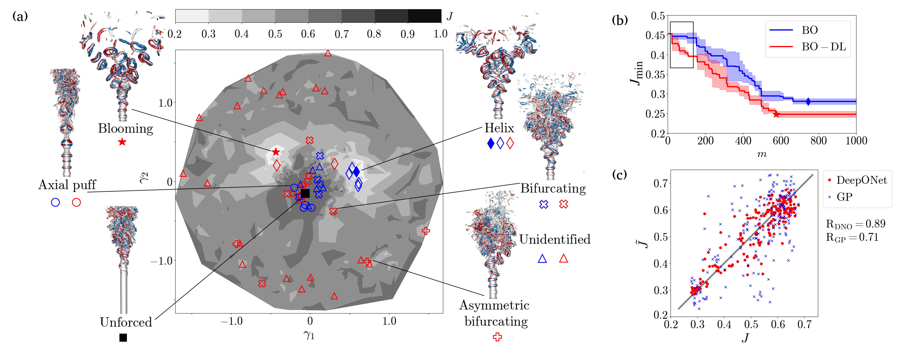
Figure 2: The learning processes of BO and BO-DL: (a) Proximity map highlighted by the unforced case (filled square), the local minima (unfilled symbols), and the final solutions explored by BO (blue-filled diamond ) and BO-DL (red-filled star), with corresponding flow patterns. (b) Average learning curves of $J_{\rm min}$. The shadowed region indicates the extrema over three realizations. (c) Prediction of $J$ by GP (cross) and DeepONet (dot).

In this section, we detail the performances and learning processes of the two optimizers after initialization, BO and BO-DL, within a budget of $1000$ evaluations. A topological analysis of the high-dimensional data set is performed following Wang et al. (2023). The analysis includes dimension reduction, data visualization, and the derivation of local minima, with the data obtained by both BO and BO-DL. The $22$-dimensional data is projected on a 2D proximity map following the approach of Li et al. (2022) by classical multidimensional scaling (Fig. 2a). The feature coordinates $\gamma_{ij}$ are chosen to optimally preserve the dissimilarity between control parameters defined by the Euclidean distance $D_{ij}=|\mathbf{b}_{i}-\mathbf{b}_{j}|$. The map features two large basins of attraction with low values of $J$, as well as small basins distributed around the border. A point $\mathbf{b}_{0}$ is supposed as a local minimum $\mathbf{m}$, if there exists a neighborhood $\mathcal{B}$ of $\mathbf{b}_{0}$ that satisfies $J(\mathbf{b}_{0})\leq\min_{\mathbf{b}\in\mathcal{B}}J(\mathbf{b})$. $\mathcal{B}$ is an open set which should include $K$ nearest neighbours of $\mathbf{b}_{0}$ measured by Euclidean distance, $K\geq N_{D}+1$. Note that the local minima are assumed based on the obtained discrete data and may change with additional data. A total of $57$ local minima are extracted from the data, with $36$ found by BO-DL and $21$ by BO. In the proximity map, the unforced case is represented by a black square where both algorithms begin. The other symbols denote the derived minima $\mathbf{m}$ found by BO (blue) and BO-DL (red). The final BO and BO-DL solutions highlighted by the filled diamond ($J=0.237$) and the filled star ($J=0.237$) are located in the large basins of attractions. Most of the minima queried by BO are located in the center of the map, whereas BO-DL also explores outward regions. Forced by the control commands corresponding to these minima, different jet patterns are observed, corroborated with the control modes. The axial puff (circles) are close to the unforced case. The bifurcating type (cross) distributes widely in the cost range. The lower the $J$ value is, the closer to the helix (filled diamond) basin. The jets bifurcating to one side are away from the center, surrounded by the other unidentified patterns (triangles). Helix (diamond) and blooming (star) jets feature the most substantial performance, but the latter is only detected by BO-DL. Among the $20$ minima explored by BO, the identified patterns include $6$ helix, $5$ flapping, and $4$ axial puff. Among the $37$ minima explored by BO-DL, the identified patterns include $6$ flapping, $5$ asymmetric flapping, $2$ helix, $1$ blooming, and $1$ axial puff. In addition, most ($22$) of the $27$ unidentified patterns are detected by BO-DL. Fig.  2(b) reports the average value of the current optimum $J_{min}=\min_{J_{i}\in\mathcal{D}_{n}}J_{i}$ from each optimizer with the standard deviation (shadows) by repeating each run $3$ times. The learning curve starts from $J_{min}=0.45$, the lowest cost value after initialization of $23$ samples including the unforced case with $J=1$. With around $570$ query points on average, BO-DL converges to the solution with a lower $J$ than BO, which takes around $750$ queries. As the rectangle denotes, the warm-up phase during $0-100$ queries with BO is significantly mitigated in BO-DL. This observation is explained by the capability of the surrogate models to predict the mixing as a response to the excitation input, $\tilde{J}(\mathbf{b})-J(\mathbf{b})$ in Fig. 2(c). A cross-validated training of the GP and DeepONet model is performed separately using a set with $1000$ data points from BO and BO-DL optimizations. The data is split into $10$ equally sized groups, with $8$ taken as the training set, and $2$ used to test the prediction. The range of $J$ value for the prediction test is approximately between $0.3$ and $0.7$. As indicated by the data along the diagonal, the $\tilde{J}$ predicted by DeepONet (dots) is closer to the truth $J$ than GP (cross). This is further explained by the correlation coefficient $R$ to quantify the regression performance, which is $0.89$ for DeepONet and $0.71$ for GP.

BO-DL explores not only more minima than BO but also more diverse flow patterns. This is probably owing to DeepONet’s capability to more accurately approximate the mapping from the high-dimensional actuation to the mixing response. Two solutions with large basins of attractions in the search space are revealed — the optimal solution with a $7$-armed blooming jet generated, and the suboptimal with a double-helix shape.

3.2 Discussion of the optimized solutions

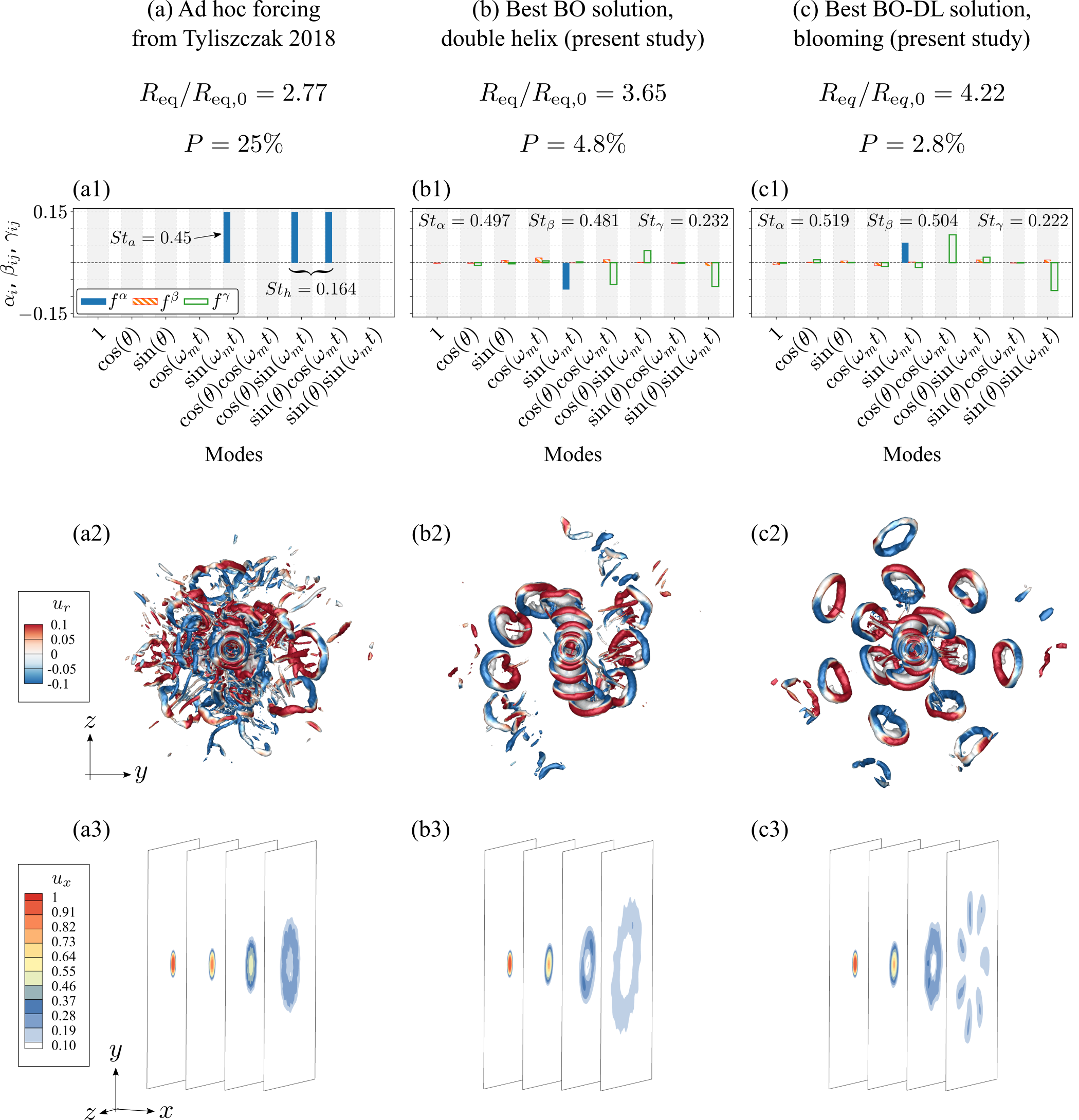
Figure 3: Comparison between three mixing jet solutions: (a) the ad hoc solution with the best mixing in Tyliszczak (2018), (b) the best solution learned with BO, and (c) the best solution learned with BO-DL. Top — forcing modes with the associated mixing and actuation metric. Middle — (contour online) bottom view of instantaneous isosurfaces of $Q=0.5$ colored by the radial velocity $u_{r}$. Bottom — (contour online) contour plots of the streamwise velocity on cross-sectional planes at $x=2D$, $4D$, $6D$, $8D$.

Here we include three solutions for the discussion: an ad hoc forcing with the best mixing in Tyliszczak (2018), BO optimized solution and the optimal solution of BO-DL. The forcing command, the instantaneous snapshots, and the mean flow fields are presented in Fig. 3. The forcing commands are expressed by the operators in an order of constant, spatial-periodic, temporal-periodic, and traveling waves in Fig. 3(a1),  3(b1) and  3(c1). The forcing commands can be shared upon request. The axial excitation combining axisymmetric and helical modes has been widely employed to study the bifurcating and blooming jets since Lee & Reynolds (1985). A parametric study of the blooming jets with this type of excitation is performed in Tyliszczak (2018), under the same Reynolds number as this study. An 11-armed jet is produced with the best mixing performance. This excitation combines the axisymmetric mode with Strouhal number $St_{a}=0.45$ and the helical mode with $St_{h}=0.164$ at the same amplitude, $15\%$ the main jet momentum flux (Fig. 3a1). The BO solution contains mainly the axisymmetric mode at an amplitude of $8\%$ with $St_{\alpha}=0.50$ for the bulk, a helical mode at an amplitude of $2\%$, and a radial-flapping mode at an amplitude of $7\%$ with $St_{\gamma}=0.23$ for radial components in the periphery. The BO-DL solution contains mainly the axisymmetric mode at an amplitude of $6\%$ with $St_{\alpha}=0.52$ for the bulk, a helical mode at an amplitude of $8\%$ with $St_{\gamma}=0.22$ for radial components in the periphery. Two significant factors to be noted are the axisymmetric forcing Strouhal number $St_{\alpha}$, and the frequency ratio between the axial and helical modes, $\alpha=St_{a}/St_{h}$. For both BO and BO-DL solutions, the axisymmetric forcing Strouhal number falls into the range $0.4\lesssim St_{a}\lesssim 0.6$ to observe bifurcating and blooming jets, and coincides with around $St_{a}=0.5$ where the peak spreading occurs (Lee & Reynolds, 1985; Shaabani-Ardali et al., 2020; Gohil et al., 2015). The BO-DL actuation takes a frequency ratio of $2.34$, in the range of $2\leq\alpha\leq 2.6$ where the blooming phenomenon is observed (Gohil et al., 2015). Interestingly, the ratio of the BO solution which produces a helix jet ($\alpha=2.14$) also falls into this range. Moreover, different from the ad hoc excitation using only the axial forcing, the radial component in the periphery plays an important role in solutions optimized by both BO and BO-DL. Shaabani-Ardali et al. (2020) also concludes radial forcing is the dominant component of helical modes to maximize the spreading angle of a bifurcating jet. We extend the importance of radial forcing to the jet spreading globally. From an estimate of the momentum flux, the solutions in this study take only $2.8\%$ (BO-DL) and $4.8\%$ (BO) of the main jet, one order lower than the ad hoc excitation ($25\%$). One reason is the low amplitudes, and another is the forcing applied into the local boundary region (see 2.2) rather than the whole jet, which leads to a more efficient control. This represents the physical reality of small actuators installed on the wall of the inlet nozzle, like flap arrays in Suzuki et al. (1999), only affecting the boundary layers.

The flow structures are presented by the bottom view of the instantaneous Q-parameter isosurfaces (Fig. 3a2, b2, and c2). The arms of the ad hoc blooming jet are not explicitly observed due to the interaction between the vortex rings aligned closely. A double-helix jet is formulated by the BO solution. The jet bifurcates into two branches and then experiences continuous bifurcation along the azimuth until the vortex rings break. This type of jet has not been reported in the literature so far. We reserve it for future investigation. The BO-DL optimized jet produces a $7$-armed blooming jet, with the vortex rings eventually propagating along $7$ different trajectories. The contour slices of the time-averaged streamwise velocity also confirm the spreading observed from the vortex rings. The 11 branches generated by the ad hoc forcing can be traced in $x=8D$. The BO-optimized jet shows more continuous distribution along the circumference due to the azimuthal bifurcation of two helix-shaped arms. The blooming jet features the earliest and furthest spreading. This leads to the largest effective mixing radius, $4.22R_{\rm eq,0}$ at $x=8D$, followed by BO optimized jet with $R_{\rm eq}=3.65R_{\rm eq,0}$, and the ad hoc forced jet with $R_{\rm eq}=2.77R_{\rm eq,0}$.

4 Conclusions

We perform a global optimization of the jet control modes, parameterized in a $22$-dimensional search space. In this study, Bayesian optimization is enriched with a deep-learning surrogate model. Thus, faster learning of better solutions is facilitated. The control landscape $J(\bm{b})$ features two persistent (pronounced) minima, a global minimum corresponding to a 7-armed blooming jet generated, and a suboptimal parameter with a double-helix shape that performs similarly. Intriguingly, many of the less persistent minima also correspond to known actuated jet mixing mechanisms.

Declaration of interests

The authors report no conflict of interest.

References

- Ball et al. (2012) Ball, C. G., Fellouah, H. & Pollard, A. 2012 The flow field in turbulent round free jets. Prog. Aerosp. Sci. 50, 1–26.
- Blanchard & Sapsis (2021) Blanchard, A. & Sapsis, T. 2021 Bayesian optimization with output-weighted optimal sampling. J. Comp. Phys. 425, 109901.
- Blanchard et al. (2021) Blanchard, A. B., Cornejo Maceda, G. Y., Fan, D., Li, Y., Zhou, Y., Noack, B. R. & Sapsis, T. P. 2021 Bayesian optimization for active flow control. Acta Mech. Sin. pp. 1–3.
- Boguslawski et al. (2019) Boguslawski, A., Wawrzak, K. & Tyliszczak, A. 2019 A new insight into understanding the crow and champagne preferred mode: a numerical study. J. Fluid Mech. 869, 385–416.
- Corke & Kusek (1993) Corke, T. C. & Kusek, S. M. 1993 Resonance in axisymmetric jets with controlled helical-mode input. J. Fluid Mech. 249, 307–336.
- Crow & Champagne (1971) Crow, S. C. & Champagne, F. H. 1971 Orderly structure in jet turbulence. J. Fluid Mech. 48 (3), 547–591.
- Danaila & Boersma (2000) Danaila, I. & Boersma, B. J. 2000 Direct numerical simulation of bifurcating jets. Phys. Fluids 12 (5), 1255–1257.
- Gohil et al. (2015) Gohil, T. B., Saha, A. K. & Muralidhar, K. 2015 Simulation of the blooming phenomenon in forced circular jets. J. Fluid Mech. 783, 567–604.
- Hilgers & Boersma (2001) Hilgers, A. & Boersma, B. J. 2001 Optimization of turbulent jet mixing. Fluid Dyn. Res. 29 (6), 345.
- Hussain & Zaman (1980) Hussain, A. K. M. F. & Zaman, K. B. M. Q. 1980 Vortex pairing in a circular jet under controlled excitation. Part 2. Coherent structure dynamics. J. Fluid Mech. 101 (3), 493–544.
- Jordan & Colonius (2013) Jordan, P. & Colonius, T. 2013 Wave packets and turbulent jet noise. Annual Review of Fluid Mechanics 45 (1), 173–195.
- Koumoutsakos et al. (2001) Koumoutsakos, P., Freund, J. & Parekh, D. 2001 Evolution strategies for automatic optimization of jet mixing. AIAA J. 39 (5), 967–969.
- Lee & Reynolds (1985) Lee, M. & Reynolds, W. C. 1985 Bifurcating and blooming jets. Tech. Rep.. Thermosciences Division, Department of Mechanical Engineering, Stanford University.
- Li et al. (2022) Li, Y., Cui, W., Jia, Q., Li, Q., Yang, Z., Morzyński, M. & Noack, B. R. 2022 Explorative gradient method for active drag reduction of the fluidic pinball and slanted Ahmed body. J. Fluid Mech. 932, A7.
- Lu et al. (2021) Lu, L., Jin, P., Pang, G., Zhang, Z. & Karniadakis, G. E. 2021 Learning nonlinear operators via DeepONet based on the universal approximation theorem of operators. Nat. Mach. Intell. 3 (3), 218–229.
- Mankbadi & Liu (1981) Mankbadi, R. & Liu, J. T. C. 1981 A study of the interactions between large-scale coherent structures and fine-grained turbulence in a round jet. Philos. Trans. Royal Soc. A 298 (1443), 541–602.
- Parekh (1989) Parekh, D. E. 1989 Bifurcating jets at high Reynolds numbers. Stanford University.
- Pickering et al. (2022) Pickering, E., Guth, S., Karniadakis, G. E. & Sapsis, T. P. 2022 Discovering and forecasting extreme events via active learning in neural operators. Nat. Comput. Sci. 2 (12), 823–833.
- Shaabani-Ardali et al. (2020) Shaabani-Ardali, L., Sipp, D. & Lesshafft, L. 2020 Optimal triggering of jet bifurcation: an example of optimal forcing applied to a time-periodic base flow. J. Fluid Mech. 885, A34.
- Shahriari et al. (2015) Shahriari, B., Swersky, K., Wang, Z., Adams, R. P. & De Freitas, N. 2015 Taking the human out of the loop: A review of bayesian optimization. Proc. IEEE 104 (1), 148–175.
- da Silva & Métais (2002) da Silva, C. B. & Métais, O. 2002 Vortex control of bifurcating jets: A numerical study. Phys. Fluids 14 (11), 3798–3819.
- Suzuki et al. (1999) Suzuki, H., Kasagi, N. & Suzuki, Y. 1999 Active control of an axisymmetric jet with an intelligent nozzle. In First Symposium on Turbulence and Shear Flow Phenomena. Begel House Inc.
- Tyliszczak (2014) Tyliszczak, A. 2014 A high-order compact difference algorithm for half-staggered grids for laminar and turbulent incompressible flows. J. Comp. Phys. 276, 438–467.
- Tyliszczak (2018) Tyliszczak, A. 2018 Parametric study of multi-armed jets. Int. J. Heat and Fluid Flow 73, 82–100.
- Utkin et al. (2006) Utkin, Y. G., Keshav, S., Kim, J. H., Kastner, J., Adamovich, I. V. & Samimy, M. 2006 Development and use of localized arc filament plasma actuators for high-speed flow control. J. Phys. D: Appl. Phys. 40 (3), 685.
- Wang et al. (2023) Wang, T., Chen, Y. Yang X., Li, P., Iollo, A., Cornejo Maceda, G. Y. & Noack, B. R. 2023 Topologically assisted optimization for rotor design. Physics of Fluids 35, 055105.
- Williams & Rasmussen (2006) Williams, C. K. & Rasmussen, C. E. 2006 Gaussian processes for machine learning. MIT press.
- Zhou et al. (2020) Zhou, Y., Fan, D., Zhang, B., Li, R. & Noack, B. R. 2020 Artificial intelligence control of a turbulent jet. J. Fluid Mech. 897, A27.