Evolution of the Size-Mass Relation of Star-forming Galaxies Since $z=5.5$ Revealed by CEERS

Abstract

We combine deep imaging data from the CEERS early release JWST survey and HST imaging from CANDELS to examine the size-mass relation of star-forming galaxies and the morphology-quenching relation at stellar masses $\textrm{M}_{\star}\geq 10^{9.5}\ \textrm{M}_{\odot}$ over the redshift range $0.5<z<5.5$. In this study with a sample of 2,450 galaxies, we separate star-forming and quiescent galaxies based on their star-formation activity and confirm that star-forming and quiescent galaxies have different morphologies out to $z=5.5$, extending the results of earlier studies out to higher redshifts. We find that star-forming and quiescent galaxies have typical Sérsic indices of $n\sim 1.3$ and $n\sim 4.3$, respectively. Focusing on star-forming galaxies, we find that the slope of the size-mass relation is nearly constant with redshift, as was found previously, but shows a modest increase at $z\sim 4.2$. The intercept in the size-mass relation declines out to $z=5.5$ at rates that are similar to what earlier studies found. The intrinsic scatter in the size-mass relation is relatively constant out to $z=5.5$.

1 Introduction

The size evolution of the stellar components of galaxies can reveal their assembly histories and how they relate to their host dark matter halos (Fall & Efstathiou, 1980; Mo et al., 1998; Kravtsov, 2013). For example, mergers of gas-poor galaxies often lead to larger systems. While major mergers yield proportionately larger remnants, minor mergers deposit more materials in the outskirt of galaxies leading to faster growth of galaxies (Bezanson et al., 2009; Naab et al., 2009). The result of this is that by including gas, size evolution becomes more complex. Slow, gas-rich mergers lead to larger disks (Robertson et al., 2006), with stellar feedback causing changes in the size independent of mergers, as a result of gaseous outflows modifying galactic potential wells (El-Badry et al., 2016). Sizes of galaxies also shed clues on properties of their dark matter halos. Galaxy sizes may be proportional to virial radii as a consequence of angular momentum conservation during the collapse of a galaxy (Mo et al., 1998; Dutton et al., 2007; Kravtsov, 2013). Furthermore, study of the scatter in galaxy sizes can be used to constrain their halo spins (Bullock et al., 2001; Macciò et al., 2008).

Observations show that galaxy sizes depend heavily on stellar mass, star-formation activity, and redshift. Holding other galaxy parameters constant, galaxy sizes are larger at lower redshift; star-forming galaxies are larger than quiescent galaxies; and size correlates with stellar mass (Kormendy & Bender, 1996; Shen et al., 2003; Ferguson et al., 2004; Trujillo et al., 2006; Buitrago et al., 2008; Conselice et al., 2011; Bruce et al., 2012; Carollo et al., 2013; Ono et al., 2013; van der Wel et al., 2014a; Lange et al., 2015; Faisst et al., 2017; Dimauro et al., 2019; Mowla et al., 2019; Nedkova et al., 2021). At intermediate stellar masses, star-forming galaxies obey a shallow relation between stellar mass and size, $\textrm{R}_{\textrm{eff}}\propto\textrm{M}_{\star}^{0.2}$, where $\textrm{R}_{\textrm{eff}}$ is the half-light radius. For quiescent galaxies, this is much steeper, $\textrm{R}_{\textrm{eff}}\propto\textrm{M}_{\star}^{0.8}$. There is noticeable scatter in the size-mass relations for both types of galaxies (van der Wel et al., 2014a; Mowla et al., 2019; Nedkova et al., 2021).

Observations also find that star-forming and quiescent galaxies have inherently different morphologies. Star-forming galaxies tend to have light distributions consistent with exponential disks with Sérsic indices $n\sim 1$, while quiescent galaxies tend to have compact light distributions with Sérsic indices $n\sim 4$ (Kauffmann et al., 2003; Baldry et al., 2006; Wuyts et al., 2011).

Most of the above studies reached a maximum redshift of $z=3$ due to limitations in the Hubble Space Telescope’s (HST) sensitivities and angular resolution. Namely, HST is limited in wavelength such that the rest-frame $V$-band is observable only up to $z=2$. Other studies have taken an alternative route by conducting measurements in the rest-frame ultraviolet (Oesch et al., 2010; Mosleh et al., 2012; Ono et al., 2013; Shibuya et al., 2015; Holwerda et al., 2015). However, these studies have conflicted with those made at rest-frame optical wavelengths van der Wel et al. (2014a) because galaxies exhibit different morphologies as a function of wavelength (e.g., Vulcani et al., 2014). It is thus crucial to measure morphological parameters at the same rest-frame wavelength across the redshift range of interest.

Furthermore, in any study involving sizes of galaxies, it is crucial to measure rest-frame sizes in a physically motivated fashion. Studies that examine the size-mass relation in the rest-frame $V$-band typically apply corrections to infer sizes that are statistical in nature, and likely not appropriate on a galaxy-by-galaxy basis (e.g., van der Wel et al., 2014a; Mowla et al., 2019). In this paper, we apply techniques developed by the MegaMorph project (Barden et al., 2012; Häußler et al., 2013; Vika et al., 2013; Häußler et al., 2022) to infer rest-frame optical morphologies for individual galaxies using multi-wavelength data.

From HST imaging data, there is a hard limit on the highest redshift observable in the rest-frame $V$-band, $z=2$. With the James Webb Space Telescope (JWST), however, we can observe the rest-frame $V$-band out to $z\sim 7$ using the NIRCam instrument, due to the significantly longer wavelengths probed by JWST at angular resolution comparable to or better than that of HST.

The Cosmic Evolution Early Release Survey (CEERS, Finkelstein et al., 2022; Bagley et al., 2023; Finkelstein et al., 2023) provides a dataset that a number of studies have recently used to examine the morphologies of galaxies at high redshift. Ferreira et al. (2023) and Kartaltepe et al. (2023) find that disk galaxies are more abundant at $z>2$ than what was expected from HST surveys. Suess et al. (2022) find that star-forming galaxies are more concentrated in terms of their stellar mass than in their rest-frame optical light at $1.0<z<2.5$ compared to previous estimates using HST data. Guo et al. (2023) find galaxy disks hosting stellar bars at redshifts as high as $z\approx 2.3$, suggesting that galaxy disks like those in the local Universe may have been in place much earlier than anticipated. Recently, Pandya et al. (2023) find that the majority of low-mass galaxies at $z>1$ are prolate, cigar-shaped systems instead of oblate disks.

This work examines the size-mass relation of star-forming galaxies and the relationship between star-formation activity and Sérsic index out to $z=5.5$. We use JWST data from CEERS, spanning an area of 97 square arcmin, as well as HST data from the Cosmic Assembly Near-Infrared Deep Extragalactic Legacy Survey (CANDELS; Grogin et al. 2011; Koekemoer et al. 2011), to select star-forming and quiescent galaxies at stellar masses greater than $10^{9.5}\ \textrm{M}_{\odot}$. We use 13 bandpasses to accurately and precisely constrain the effective radii and Sérsic indices at rest-frame 5,000Å of more than 2,000 galaxies to $z=5.5$.

This paper is structured as follows. In Section 2, we describe the data we use in this paper. In Section 3, we list the cuts we apply to select our sample of galaxies. Section 4 describes our measurements of galaxy morphologies and the associated uncertainties, classification of galaxies into star-forming and quiescent systems, and how the size-mass relation is estimated. The analysis of the size-mass relation and the morphology-quenching relation is described in Section 5. We interpret our results in Section 6. We conclude in Section 7.

In this paper, we assume a $\Lambda$CDM cosmology with $\Omega_{\Lambda}=0.3$, $\Omega_{M}=0.7$, and $H_{0}=70\ \textrm{km s}^{-1}\ \textrm{Mpc}^{-1}$. All magnitudes are in the AB photometric system (Oke & Gunn, 1983).

2 Data

2.1 CANDELS and CEERS Imaging

The CEERS Team has provided high quality mosaics as a part of the JWST Early Release Science (ERS) program (Finkelstein et al., 2022). The CEERS mosaics cover 97 sq. arcmin and overlap with the Extended Groth Strip (EGS), a Hubble Space Telscope (HST) legacy field. Mosaics in 13 bandpasses are used in this work: F606W and F814W (ACS); F105W, F125W, F140W, and F160W (WFC3); and F115W, F150W, F200W, F277W, F356W, F410M, and F444W (NIRCam). We include HST data from CANDELS (Grogin et al., 2011; Koekemoer et al., 2011) so that the rest-frame $5,000$Å is sampled at the lowest redshifts considered in this work. The 5$\sigma$ depths in each filter are correspondingly 28.62 and 28.30 (ACS); 27.11, 27.31, 26.67, and 27.37 (WFC3); 29.15, 29.00, 29.17, 29.19, 29.17, 28.38, and 28.58 mag (NIRCam). All mosaics have a pixel scale of 30 milli-arcseconds. The CEERS survey observed the EGS field in 10 NIRCam pointings. Objects are detected in an error-weighted mosaic of the F277W and F356W bandpasses.

Data reduction was performed by Bagley et al. (2023). In short, JWST Calibration pipeline v1.7.2 and CRDS pmap 0989 were used to process the pointings from June 2022, whereas JWST Calibration pipeline v1.8.5 and CRDS pmap 1023 were used to process pointings from December 2022. For all pointings, the images were reduced using a custom pipeline developed by the CEERS team, which includes $1/f$ noise subtraction and snowball removal. Lastly, the mosaics were aligned using astrometry from Gaia-EDR3 (Gaia Collaboration et al., 2021), mapped to a pixel scale of 0.03”/px, and finally background subtracted.

We adopt simulated NIRCam point spread functions (PSFs) generated using WebbPSF (Perrin et al., 2014). The PSF full-width at half-maximum (FWHM) of the JWST NIRCam bandpasses used here ranges from 0.040” to 0.145”. The HST ACS and WFC3 bandpasses used in this work have PSF FWHM ranges from 0.10” to 0.19” Skelton et al. (2014).

2.2 Photometric Redshifts, Rest-Frame Colors, and Stellar Masses

Photometric redshifts and rest-frame colors for our sample are estimated using eazy (Brammer et al., 2008) and adopted from the fits performed by Barro et al. (2023). eazy measures photometric redshifts by fitting non-negative linear combinations of templates to photometric observations and derives probability distribution functions of the redshift. Templates are supplied by users. For our sample, we adopt the standard “tweak_fsps_QSF_12_v3” templates, which are made of 12 flexible stellar population synthesis (FSPS, Conroy & Gunn 2010) templates, as recommended by the eazy documentation. A prior on the fluxes of galaxies in F277W is assumed to assign low probabilities at very low redshifts and for bright galaxies at very high redshifts.

eazy is run on a flux-limited subset of the CEERS catalog (see Section 3). To assess the accuracy of the photometric redshifts inferred by eazy, we compare these against spectroscopic redshifts of 1,187 galaxies in the All-Wavelength Extended Groth Strip International Survey (AEGIS; Davis et al. 2007) that were compiled by Stefanon et al. (2017, see references therein). We use the bias and scatter scatter using the normalized median absolute deviation (NMAD) to quantify the accuracy of the photometric redshifts (Dahlen et al., 2013). We find a bias of -0.01, such that the photometric redshifts very slightly overestimate the spectroscopic redshifts, and $\sigma_{\textrm{NMAD}}=0.02$.

Stellar masses for the galaxies in our sample are estimated using fast (Kriek et al., 2009) and are also adopted from Barro et al. (2023). Exponentially declining star-formation histories are assumed and the minimum star-formation history timescale is set to $\log\tau\ (\textrm{yr})=8.5$. The metallicity is fixed to solar and a Calzetti et al. (2000) attenuation curve is assumed. The Bruzual & Charlot (2003) stellar population synthesis templates are assumed and the initial mass function is set to that by Chabrier (2003).

3 Sample Selection

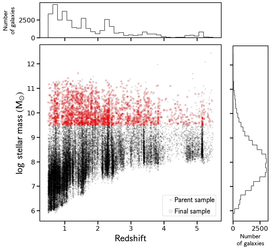
Figure 1: The distribution of the parent and final samples (see Section 3 in terms of stellar mass and redshift and over the redshift range examined in this paper, $0.5<z<5.5$. The parent sample is displayed as black dots and the final sample is shown as empty red squares. The redshift and stellar mass distributions of the parent sample are presented as histograms in the top panel and right panels, respectively. We estimate a stellar mass completeness limit of $\sim 10^{8}\ \textrm{M}_{\odot}$.

We start with all sources in the CEERS photometry catalog (v0.51.2). There is a total of 101,808 sources. We first select sources that are brighter than 28.5 mag in F356W. This cut removes 47,923 objects and leaves 53,885. These 53,885 galaxies are the parent sample from which we shall produce our final sample. The parent sample is shown in Figure 1 as black dots.

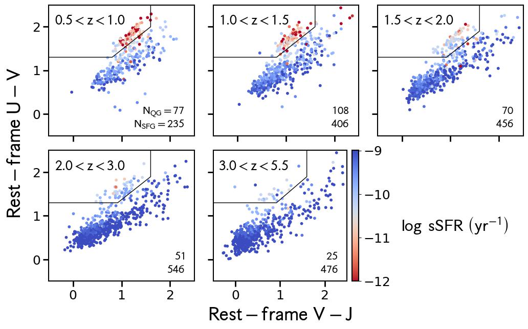
Figure 2: Rest-frame U-V and V-J color distributions of the sample examined in this paper. We split our sample into five redshift bins, which are indicated in the top left corner of each panel. Galaxies are colored by sSFR, which is measured by SED fitting (see Section 3). Quiescent galaxies are indicated by red points. Color selection criteria for quiescent galaxies developed by Williams et al. (2009) are indicated by the thin lines. Galaxies are considered quiescent if they lie within these lines. The selection criteria by Williams et al. (2009) recover well the color-color distributions of quiescent galaxies out to $z\sim 3$. The numbers of quiescent and star-forming galaxies in each redshift bin are shown in the bottom right corner of each panel.

We remove unresolved point sources and stars by following the procedure as described in Section 3 by Holwerda et al. (2023). Unresolved objects are identified by comparing the half-light radius in F200W, measured by Source Extractor, against the F200W magnitude. Stars and unresolved objects lie on a tight sequence of compact objects that extends to bright magnitudes. We denote the stellar locus in this parameter space using

$$\left|R_{h,F200W}+0.001m_{F200W}+0.065\right|<0.01,$$

where $R_{h,F200W}$ is the half-light radius in arcsec and $m_{F200W}$ is AB magnitude. The inequality above applies only to objects brighter than 28th magnitude in F200W. There are 572 objects that are removed as they lie on the stellar locus, which leaves 53,313 galaxies remaining.

The main goal of this work is to determine the evolution with redshift of the rest-frame optical size-mass relation of star-forming galaxies. Sizes are measured in the rest-frame $5,000$Å to be consistent with previous studies. To ensure that there is at least one bandpass at shorter and longer wavelengths than the rest-frame $5,000$Å for each galaxy, we select galaxies at redshifts $0.5\leq z\leq 5.5$. This cut excludes 15,721 galaxies with 37,592 remaining.

This work relies on the morphological measurements of galaxies spanning a wide range in redshift. To ensure high S/N in as many bandpasses as possible, we select galaxies with stellar mass $>10^{9.5}\ \textrm{M}_{\odot}$. Over the redshift range examined in this work, we estimate the completeness limit in mass to be $\sim 10^{8}\ \textrm{M}_{\odot}$, similar to what Huertas-Company et al. (2023) found. This limit can be seen as the peak in the histogram in the right side panel of Figure 1. This cut in stellar mass is well above our estimated completeness limit and reduces the sample by 34,798 and leaves 2,794 galaxies.

We remove galaxies hosting active galactic nuclei (AGN), which may not be fitted well with one-component Sérsic models, as follows. To remove X-ray-detected AGN, we match our catalog to the Chandra X-ray catalog produced by Nandra et al. (2015). These observations reach a typical depth of 800 ks across the EGS field. We use a search radius of 0.5 arcsec and find 91 matches to the Nandra et al. (2015) catalog, 74 of which are in our mass-selected sample above. All 74 of these matches are removed from our sample, leaving 2,720 galaxies.

Early JWST surveys revealed a new population of compact objects with blue SEDs at short wavelengths and very red SEDs at long wavelengths (Barro et al., 2023; Labbé et al., 2023; Matthee et al., 2023). The colors of such objects can be explained by combining dust-reddened quasar light with bluer light from young stellar populations. Due to the puzzling nature of such objects, we apply a strict color cut of F277W - F444W $>$ 1.5, which we adopt from Barro et al. (2023), to remove these objects. This cut excludes 11 galaxies and 2,709 remain.

Since this work aims to simultaneously fit HST and JWST images of a sample of galaxies, we remove galaxies that are not detected in HST images. There are 50 such galaxies removed from the sample, which leaves 2,659.

We visually inspected these 2,659 galaxies for bright neighboring galaxies or stars that could adversely affect the 2D Sérsic fits, galaxies lying on the edge of the mosaic, and spurious sources that were identified by the hot Source Extractor run as described in Section 3. We remove 132 galaxies: 35 are removed due to having bright nearby stars; 77 are removed due to their proximity to the edge of the mosaic; and 20 are removed due to being spurious sources. After excising these sources, 2,527 galaxies remain.

To remove objects that have poor fits with large residuals, we use a cut in the residual flux fraction (RFF, see Section 4.2). A large RFF signifies that much of the light in the galaxy is not adequately modeled, and hence morphological parameters may be inaccurate (e.g., bright spiral arms and bars that are not accounted for in 2D Sérsic fits). We reject objects with $\left|RFF\right|>0.5$ which excludes 15 galaxies due to large residuals, leaving 2,512 galaxies. We also exclude 62 galaxies that have Sérsic indices that lie beyond the bounds we set for our fits ($0.3<n<8$) or effective radii that are too small or too large (sizes must lie between 0.009” and 3”), with 2,450 remaining.

The final sample contains 2,450 galaxies. These are shown as red empty squares in Figure 1 in terms of stellar mass and redshift. In Figure 2, the final sample is displayed in rest-frame UVJ color-color diagrams and in five redshift bins. The galaxies in our sample populate the regions of color-color space spanned by star-forming and quiescent galaxies (see Section 4.4).

4 Methods

4.1 Two-dimensional Sérsic Model Fitting

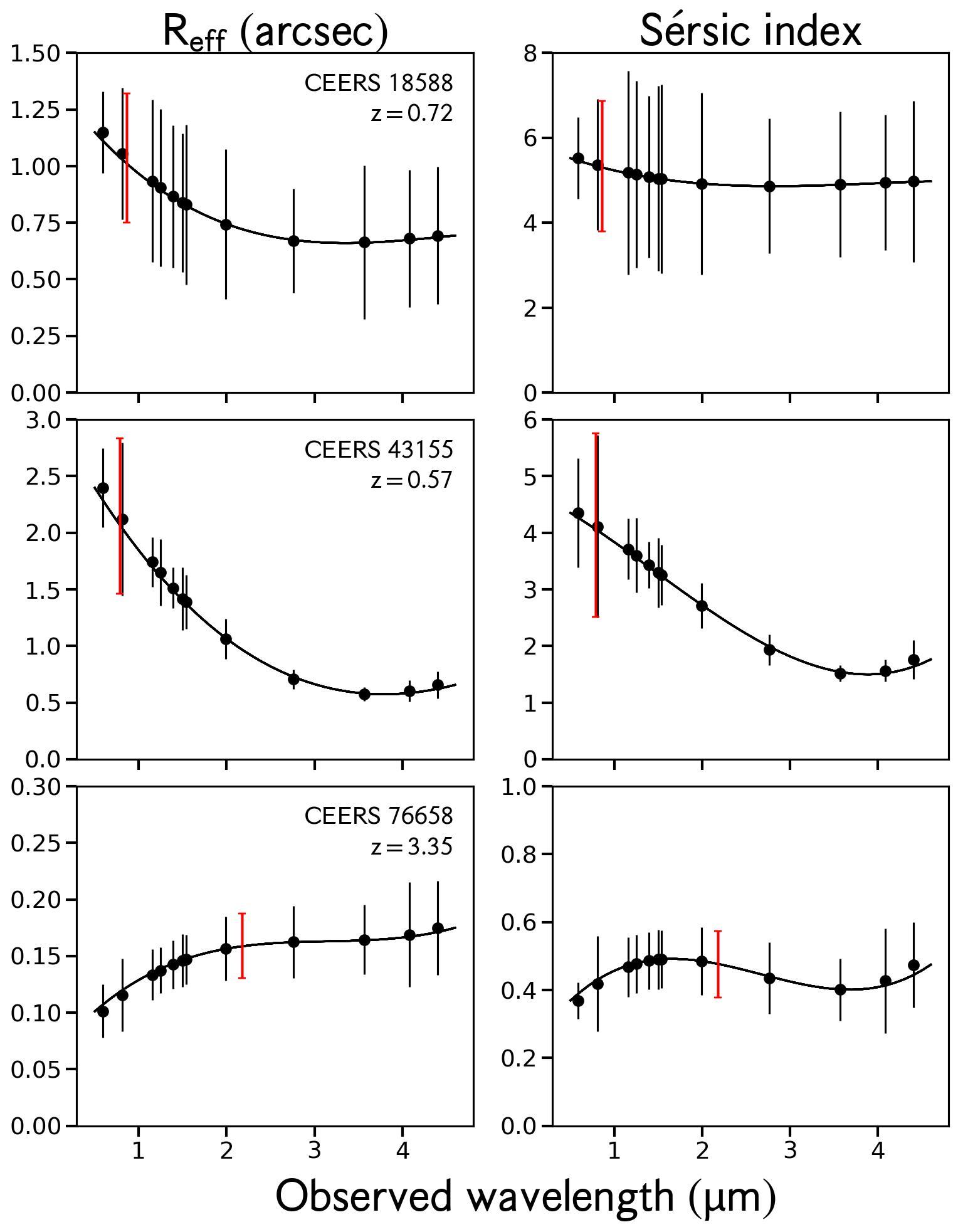
Figure 3: Multi-wavelength fits to three example galaxies. Fits for a different galaxy are shown in each row. Measurements in each bandpass from the fits are shown as dots with error bars. Effective radii and Sérsic indices in different bandpasses are shown in the left and right columns, respectively. The third-order fits to the images are shown as solid lines. Red error bars indicate parameters in the rest-frame $5,000$Å derived from the multi-band fits.

We use the galfitm tool (Barden et al., 2012; Häußler et al., 2013; Vika et al., 2013; Häußler et al., 2022) to perform simultaneous multi-wavelength morphological fits of galaxies in our sample. galfitm is used as it has been shown that morphological fits using this tool result in more stable and accurately measured parameters (Häußler et al., 2013). galfitm is built upon the galfit code (Peng et al., 2002, 2010), which performs morphological fits to images in individual bandpasses. Morphologies are quantified with two-dimensional (2D) Sérsic functions (Sersic, 1968), which are then convolved with the PSF at different wavelengths.

We construct error maps for each bandpass, which take into account Poisson noise from galaxies, instrumental noise, and errors due to background subtraction. For the NIRCam bandpasses, these error maps have been produced by the CEERS team (see Bagley et al., 2023, for more details). For the HST bandpasses, we estimate these maps following the procedure as described in Section 4.1 by van der Wel et al. (2012), which makes use of exposure time mosaics and weight maps.

The images used to perform the fits are cutouts from the HST and JWST mosaics. Each cutout is square and has side length equal to 20 times the half-light radius measured by Source Extractor in the F200W bandpass. For each galaxy in our sample, we also fit neighboring galaxies that are at least half as bright as the target galaxy in F356W, which is the redder bandpass used to detect galaxies in CEERS (see Section 2). Neighboring galaxies are fitted provided they lie within the extent of the cutout of the target. Fainter objects are masked out using segmentation maps determined by Source Extractor.

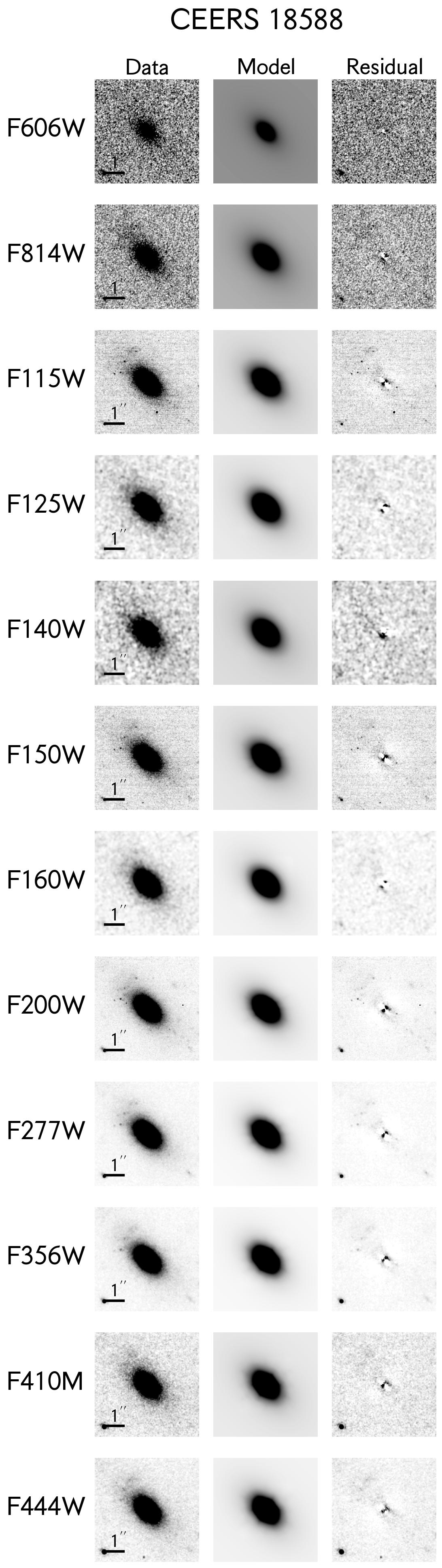
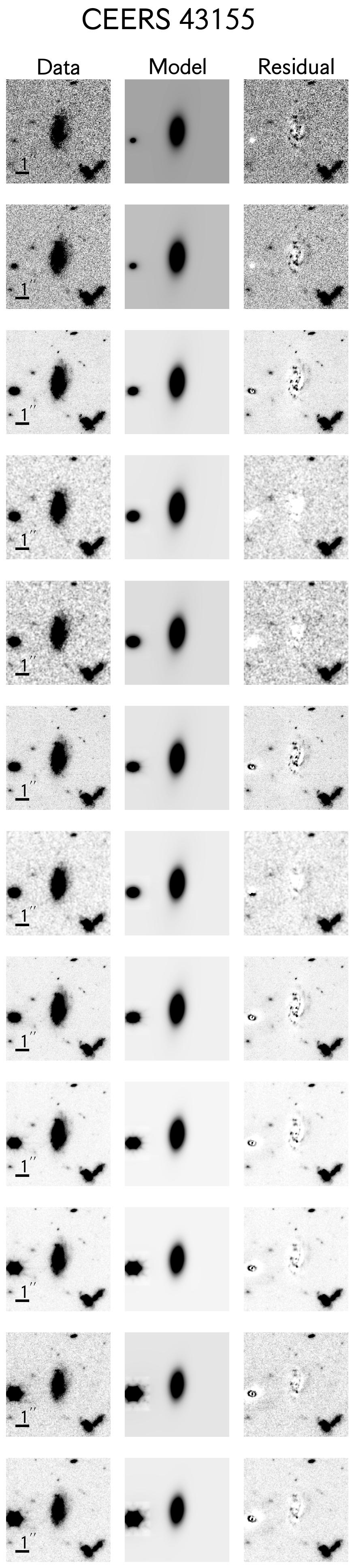
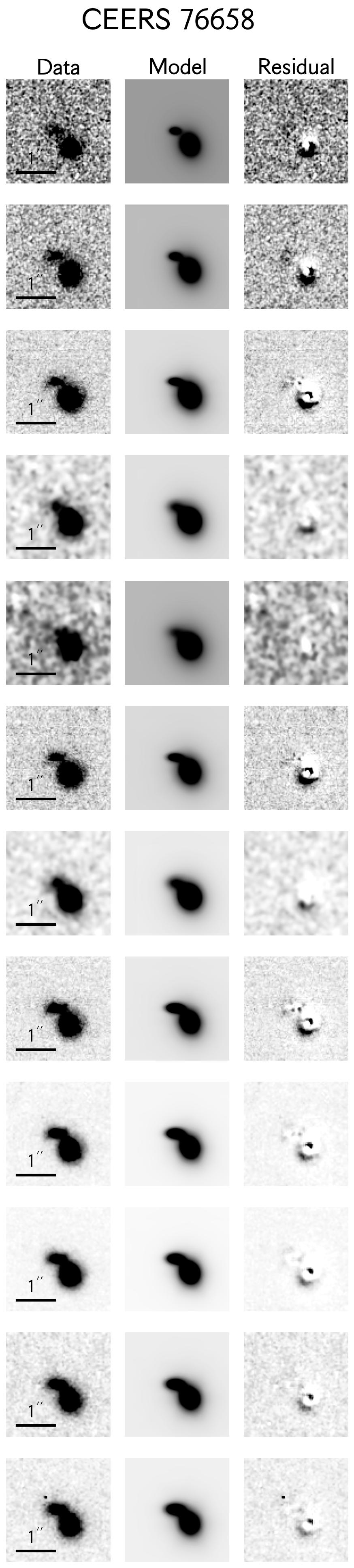
Figure 4: Multi-wavelength fits to the same three example galaxies shown in Figure 3. In each set of three columns, the left column displays postage stamps in all 12 bandpasses in which each galaxy is observed. The black bars in the lower left corner of each set of plots indicate an angular scale of 1 arcsec. None of these galaxies were observed in F105W, thus we do not show the fits in that bandpass. In the middle columns are the best-fitting models in each bandpass derived from the simultaneous multi-band fits. In the rightmost columns are images of the residuals, i.e., the models subtracted from the data. Our fits perform well in general, and bright neighbors are fit well, as can be seen in the fits for CEERS 43155 and 76658.

For our simultaneous multi-wavelength fits, we largely follow what is commonly done in the literature, albeit with some modifications. Earlier studies that performed multi-wavelength fits use up to seven bandpasses in their fits and often assume second-order polynomials to model both the effective radius and Sérsic index as a function of wavelength (Häußler et al., 2013; Vika et al., 2013; Nedkova et al., 2021). This is done as galaxies are observed to vary in size and compactness as a function of wavelength, due to, e.g., the presence of a bulge or disk (e.g., Vulcani et al., 2014).

After trial and error, we instead assume third-order polynomials to model both the effective radius and Sérsic index as a function of wavelength. For many galaxies, we find that their effective radii and Sérsic indices, when plotted as a function of wavelength, present at least one inflection point. Examples of multi-wavelength fits are shown for three galaxies as points with error bars in Figure 3. In particular, for CEERS 43155, displayed in the middle row, its Sérsic index as a function of wavelength decreases steeply from $\sim 0.6$ to $\sim 3\mu\textrm{m}$ and is nearly constant at longer wavelengths. Modeling this behavior is difficult if second-order polynomials are assumed, whereas third-order polynomials have enough degrees of freedom to fit data like these.

Following Nedkova et al. (2021), the axis ratio, central coordinates, and position angle are each fitted to constant values that do not depend on wavelength. Following Häußler et al. (2013), we also assume Chebyshev polynomials of the first kind (Abramowitz & Stegun, 1965) in the multi-wavelength fits. The magnitudes of the models as a function of wavelength are left to vary freely in all 13 bandpasses. There are thus 25 free parameters in total for each multi-wavelength fit. For all galaxies, we restrict the effective radius in each bandpass to lie between 0.3 and 100 pixels (0.009 and 3 arcsec) and the Sérsic index to lie between 0.3 and 8.

Examples of multi-wavelength fits are shown in Figure 4 for the same galaxies whose fitted parameters are shown in Figure 3. For each galaxy, there are three columns. The left column shows the galaxy in each bandpass from top to bottom in order of increasing wavelength. The middle column shows the best-fitting model from the multi-wavelength fit. The right column shows the model subtracted from the galaxy image, i.e., the residual image. In general, our fits perform well. One galaxy, CEERS 76658, is fitted well despite a bright and close neighbor. This suggests that our masking technique results in reasonable fits. For most fits, residuals of the order of 10% remain, but these are expected, given that one-component Sérsic models are likely not the most appropriate description of the morphologies of most galaxies (Peng et al., 2002). In Appendix A, we compare our multi-wavelength fits to fits that are performed bandpass-by-bandpass by McGrath et al. (in prep.) using galfit. We find good agreement between their fits and ours.

4.2 Residual Flux Fraction

To identify galaxies with poor morphological fits and remove them from our sample, we use the residual flux fraction (RFF; see Section 3). The RFF is a measure of the signal in the residual image that cannot be attributed to fluctuations in background sky values (Hoyos et al., 2012). Following Margalef-Bentabol et al. (2016), we define the RFF as:

$$RFF=\frac{\sum\limits_{j,k\in A}\left|I_{j,k}-I_{j,k}^{GALFITM}\right|-0.8\sum\limits_{j,k\in A}\sigma_{B_{j,k}}}{FLUX\textunderscore AUTO}$$

where $I_{j,k}$ is the flux in the $j$th and $k$th pixels in the science image, $I^{GALFITM}$ is the model image estimated by galfitm, $\sigma_{B}$ is the background error due to sky subtraction, and FLUX_AUTO is the flux of the galaxy calculated by Source Extractor. These are all in the bandpass that is closest to the rest-frame 5,000Å of the galaxy.

The factor of 0.8 in the numerator ensures that the average value of the RFF vanishes to zero when a Gaussian error image with constant variance is encountered (Hoyos et al., 2011). We calculate the RFF within an elliptical aperture of radius equal to 1.5 times the Kron radius, where we define the Kron radius as the semi-major axis of the Kron ellipse. Calculating the RFF over a large radius leads to the RFF decaying to zero, where the outer areas can dominate the calculation, even if there is a complex residual at the centre of the image. Any neighboring sources within the Kron aperture are masked.

We calculate the background sigma term following Margalef-Bentabol et al. (2016):

$$\sum\limits_{j,k\in A}\sigma_{B_{j,k}}=N\langle\sigma_{B}\rangle$$

where $\langle\sigma_{B}\rangle$ is the mean value of the sky background. This is estimated by computing the mean flux estimated by placing empty apertures in random locations of the background-subtracted science image. The value of $N$ is the number of pixels within the Kron aperture that we describe above.

4.3 Morphological Parameter Uncertainties

We follow the technique developed by van der Wel et al. (2012), albeit with minor changes, to compute uncertainties in individual bandpasses on the effective radii and Sérsic indices derived from the multi-wavelength fits. Uncertainties on rest-frame quantities are obtained by taking relative errors on the parameters in the bandpass that is closest to the rest-frame $5,000$Å at the redshift of each galaxy in our sample.

Uncertainties on the effective radii and Sérsic indices in individual bandpasses are derived as follows. Following Sec. 5.1 by van der Wel et al. (2012), for each galaxy in our sample, we first search for galaxies with derived properties most similar to the target galaxy in a given bandpass. This is done by computing the Euclidean distance

$$p_{i,j}=$$

$$\sqrt{\left(\frac{m_{i}-m_{j}}{\sigma m}\right)^{2}+\left(\frac{\log n_{i}-\log n_{j}}{\sigma(\log n)}\right)^{2}+\left(\frac{\log r_{i}-\log r_{j}}{\sigma(\log r)}\right)^{2}},$$

where $m_{i},n_{i}$, and $r_{i}$ are the magnitude, Sérsic index, and effective radius of the target galaxy, and parameters with subscript $j$ denote parameters pertaining to another galaxy in the sample. In the equation above, $\sigma$ denotes the standard deviation of the respective parameter. Hence, these distances are dimensionless and normalized relative to the distribution of parameters in the sample.

For the 11 galaxies most similar to the target galaxy, i.e., the 11 galaxies with the smallest $p_{i,j}$ as defined above, we do the following. First, we compute the differences in each parameter between these 11 galaxies and the target galaxy. Then, we compute the difference between the 16th and 84th percentiles of the distribution of differences defined above. This difference between the 16th and 84th percentiles, $q_{i,j}$ ($\delta_{i,j}$ in van der Wel et al. 2012), is computed for each galaxy in our sample. We account for the S/N of the target by multiplying $q_{i,j}$ by the S/N of the target.

We determine uncertainties on the parameters as follows. First, we find the 25 nearest galaxies to a target galaxy using $p_{i,j}$ defined above. For these 25 nearest galaxies, we find the average $q_{i,j}$, as described earlier, and divide by the S/N of the target.

For the computations described above, we keep the effective radii and Sérsic indices in logarithmic units and leave magnitudes as they are. The final uncertainties on the parameters are converted to linear units, e.g., $\delta r=\ln(10)r\delta\log r$. This procedure yields relative errors ($\lesssim 15\%$) that are consistent with what is found in Table 2 by van der Wel et al. (2012) and Table A1 by Nedkova et al. (2021) for galaxies with F160W magnitudes $<26$, as is appropriate for our sample.

The minor differences between the procedure above and what van der Wel et al. (2012) do are as follows. van der Wel et al. (2012) have a parent sample that is $\approx 2.5$ times larger than ours (6,492 vs. 2,450). These authors select the 200 closest galaxies to the target prior to computing $q_{i,j}$, whereas we select the 11 closest. We downscale this number of 200 to 11 to make it more appropriate for our sample as follows. We first scale down this number by taking the ratio of the size of the sample used by van der Wel et al. (2012) and ours (6492 / 2450). We then take the cube of this ratio as the Euclidean distance $p_{i,j}$ is calculated in three dimensions. van der Wel et al. (2012) compute $q_{i,j}$ using the differences between parameters inferred from deep and shallow imaging in CANDELS, whereas we calculate $q_{i,j}$ using the differences between the parameters of the 11 closest galaxies to the target and those of the target itself. In essence, our uncertainties are computed by estimating the ensemble properties of galaxies that are similar to a target galaxy.

For uncertainties on the rest-frame parameters, we assume the relative uncertainties in the bandpasses closest to the rest-frame 5,000Å at the redshifts of the galaxies in our sample. To obtain the total uncertainties on the rest-frame parameters, we multiply these relative uncertainties by the parameters inferred from the mutli-wavelength fits at the wavelengths that correspond to the rest-frame 5000Å. This approach is similar to what Nedkova et al. (2021) do, who instead compute uncertainties in rest-frame optical quantities by interpolating between the uncertainties on the parameters in the bandpasses that surround the rest-frame 5,000Å. Parameters and their respective uncertainties in the rest-frame 5000Å are shown as red vertical error bars in Figure 3.

4.4 Separating Star-forming and Quiescent Galaxies using the Rest-frame UVJ Color-color Diagram

Galaxies are often separated into star-forming and quiescent using the rest-frame U-V and V-J colors (e.g., Williams et al., 2009; Whitaker et al., 2011). These colors are often interpreted as indicators of the age and dust content of a stellar population, respectively. We adopt the redshift-dependent color-color criteria developed by Williams et al. (2009) to identify quiescent galaxies. These criteria are motivated by the observed distribution of galaxies in color-color space as a function of redshift.

The rest-frame UVJ colors of galaxies in our sample are shown in Figure 2. Galaxies are presented as dots colored by log(sSFR), with blue and red colors indicating high and low sSFR, respectively in Figure 2. The selection criteria by Williams et al. (2009), shown as thin dark lines, separate quiescent and star-forming galaxies, which correspond to red and blue dots, respectively. Despite the few quiescent galaxies observed at $3.0<z<5.5$, galaxies with the lowest sSFRs at these redshifts tend to lie within the selection region.

To check the nature of these putative quiescent galaxies, we determine which galaxies lie in the observed F150W-F277W, F277W-F444W color-color selection wedge developed by Long et al. (2023). These authors determined where in this observed color-color space quiescent galaxies at $3<z<6$ lie. We find that 20 of the 25 galaxies in the quiescent region in the UVJ diagram at $3.0<z<5.5$ lie in the Long et al. (2023) wedge. This suggests that, at least for the sample of galaxies examined in this work, our selection criteria perform well over the entire redshift range we examine.

4.5 Measuring the Size-mass Relation for Star-forming Galaxies

The goal of this work is to determine the evolution of the relationship between effective radius and stellar mass with redshift for star-forming galaxies out to $z=5.5$. Star-forming galaxies are selected for these measurements as quiescent galaxies become increasingly rare with increasing redshift. The cuts we have applied result in too few quiescent galaxies in each redshift bin to adequately measure the mass-size relation for quiescent galaxies.

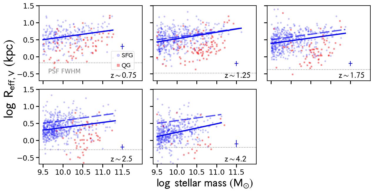
Figure 5: The relation between the size at rest-frame 5,000Å and stellar mass of galaxies in our sample as a function of redshift. Star-forming galaxies and quiescent galaxies are shown as small blue dots and small red squares, respectively. Redshift increases from left to right. The median redshift in each bin is indicated in the lower right corner of each panel. The mean uncertainties in size and stellar mass are indicated by the error bars in the lower right corner of each panel. The best-fit size-mass relations are plotted as solid blue lines. The dashed blue line is the best-fitting relation at $z\sim 0.7$ plotted in the other bins for comparison. We find that the slope is roughly constant out to $z\sim 2.5$ and shows a minor increase at $z\sim 4.2$. The PSF FWHM of the bandpass that is closest to $5,000$Å in the rest frame is shown in dotted lines in each panel. Only a handful of galaxies in our sample have sizes that are comparable to the PSF FHWM in each redshift bin.

Following earlier studies (van der Wel et al., 2014a; Dimauro et al., 2019; Mowla et al., 2019; Nedkova et al., 2021), we parameterize the size-mass relation by assuming a linear relation between the logarithm of the stellar mass and the logarithm of the effective radius in units of kpc and in the rest-frame 5,000Å, or more simply, a power law. The parameters of this linear relation are the intercept at a stellar mass of $5\times 10^{10}\ \textrm{M}_{\odot}$ and the slope. Following van der Wel et al. (2014a), we can also measure the intrinsic scatter of the size-mass relation under the assumption that it behaves like a log-normal distribution (i.e., assume Gaussian scatter when fitting the log of the mass and size).

We fit for these three parameters (intercept A, slope $\alpha$, and intrinsic scatter $\sigma_{\log\ \textrm{Reff}}$) using a Markov Chain Monte Carlo (MCMC) approach following Nedkova et al. (2021). We use the emcee tool (Foreman-Mackey et al., 2013) to estimate the posterior distributions for each parameter. Priors are assumed to be uniform with the range on each prior set to [-1.0, 1.5], [0.0, 2.0], and [0.0, 2.0] on log A, $\alpha$, and $\sigma\left(\log\ \textrm{R}_{\textrm{eff}}\right)$, respectively. In each redshift bin, we run emcee using 50 walkers for 11,000 steps and discard the first 1,000 steps.

To prevent low-mass galaxies from biasing the fit due to their greater abundance relative to high-mass galaxies, we apply a mass-dependent weight $W$, which is the inverse of the number density of galaxies at a given mass and redshift. We adopt the stellar mass functions measured by Davidzon et al. (2017) to calculate the weights. To account for outliers and mis-classification of star-forming galaxies, we assume an outlier fraction ($P_{out}$) of 5% and mis-classification probability ($C$) equal to 10%.

We compute two variance terms in the likelihood calculation: one term that combines the errors on the effective radii of individual galaxies $e$ and the intrinsic scatter in the size-mass distribution:

$$\sigma_{\textrm{eff}}^{2}=\sigma_{\log\ \textrm{Reff}}^{2}+e^{2}.$$

Another variance term combines the errors on the effective radii of galaxies and the mis-classification probability:

$$\sigma_{\textrm{mis}}^{2}=C^{2}+e^{2}.$$

The likelihood we maximize is

$$\mathcal{L} =\sum\ln\left[(1-P_{out})\cdot W\right]-\frac{1}{2}\ln\left[2\pi\sigma_{\textrm{eff}}^{2}\right]$$

$$-\frac{1}{2}\left[\log\textrm{R}_{\textrm{eff}}-\left(\log(A)+\alpha\cdot\left[\log\textrm{M}_{\star}-10.7\right]\right)\right]^{2}/\sigma_{\textrm{eff}}^{2}$$

$$+\ln P_{out}-\frac{1}{2}\ln\left[2\pi\sigma_{\textrm{mis}}^{2}\right]$$

$$-\frac{1}{2}\left[\log\textrm{R}_{\textrm{eff}}-\left(\log(A)+\alpha\cdot\left[\log\textrm{M}_{\star}-10.7\right]\right)\right]^{2}/\sigma_{\textrm{mis}}^{2},$$

where $\log\textrm{M}_{\star}$ here represents the stellar masses of the galaxies in a given redshift bin. We maximize the likelihood separately for the galaxies in each redshift bin and record the best-fitting intercept, slope, and intrinsic scatter. We discuss the results of these fits in the next section.

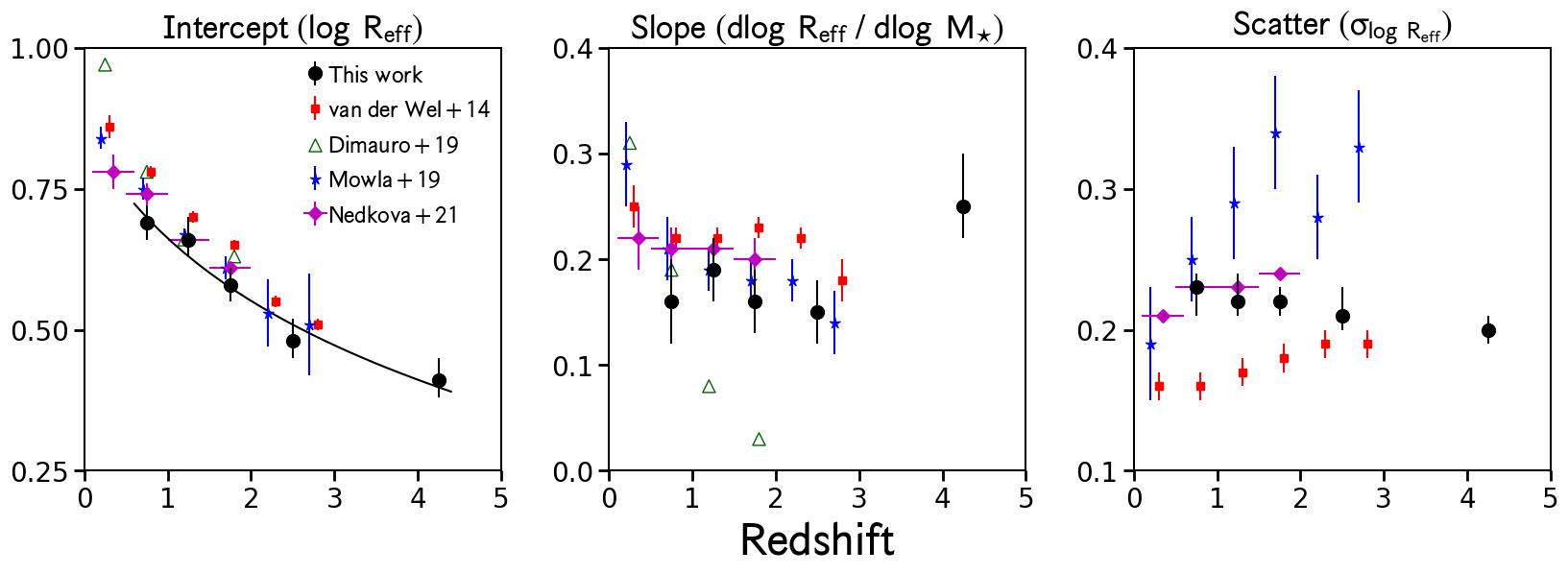
Figure 6: Left: best-fitting intercepts at a stellar mass of $5\times 10^{10}\ \textrm{M}_{\odot}$ of the size-mass relations for star-forming galaxies shown in Figure 5 as a function of redshift. Middle: best-fitting slopes of the size-mass relations. Right: Intrinsic scatter in the size-mass relations. Results from the literature are shown in various symbols. Results by van der Wel et al. (2014a); Dimauro et al. (2019); Mowla et al. (2019) and Nedkova et al. (2021) are also shown at the redshifts and stellar masses where these studies and ours overlap. Results from these studies are presented as red squares, empty green triangles, blue stars, and magenta diamonds, respectively. Results obtained by van der Wel et al. (2014a) and Mowla et al. (2019) are shifted in redshift by +0.05 and -0.05, respectively, for clarity. Please see the text for more details. We find that galaxies become smaller with increasing redshift. The solid line is a power-law fit to the intercept at $\textrm{M}_{\star}=5\times 10^{10}\ \textrm{M}_{\odot}$ as a function of redshift, $\textrm{R}_{\textrm{eff}}\ /\ \textrm{kpc}=7.1(1+z)^{-0.63}$.The size-mass relation of star-forming galaxies has a steeper slope at $z>2.5$ than it does at lower redshifts. The scatter in the size-mass relation is relatively constant out to $z=5.5$.

Table 1: Best-fit Results of the Size-mass Relation of Star-forming Galaxies of the Form $\textrm{R}_{\textrm{eff}}\ /\ \textrm{kpc}=A\left(\textrm{M}_{\star}/5\times 10^{10}\textrm{M}_{\odot}\right)^{\alpha}$ as Shown in Figures 5 and 6

Redshift range	Intercept $\log(A)$	Slope ($\alpha$)	$\sigma\left(\log\ \textrm{R}_{\textrm{eff}}\right)$
$0.5<z<1.0$	$0.69_{-0.03}^{+0.03}$	$0.16_{-0.04}^{+0.04}$	$0.23_{-0.02}^{+0.01}$
$1.0<z<1.5$	$0.66_{-0.03}^{+0.04}$	$0.19_{-0.03}^{+0.03}$	$0.22_{-0.01}^{+0.02}$
$1.5<z<2.0$	$0.58_{-0.03}^{+0.03}$	$0.16_{-0.03}^{+0.03}$	$0.22_{-0.01}^{+0.01}$
$2.0<z<3.0$	$0.48_{-0.03}^{+0.04}$	$0.15_{-0.03}^{+0.03}$	$0.21_{-0.01}^{+0.02}$
$3.0<z<5.5$	$0.41_{-0.03}^{+0.04}$	$0.25_{-0.03}^{+0.05}$	$0.20_{-0.01}^{+0.01}$

5 Results

5.1 The Stellar Mass-Size Relation of Star-forming Galaxies out to $z=5.5$

We show stellar mass against effective radii at rest-frame 5,000Å for both star-forming and quiescent galaxies as blue dots and red squares, respectively, in Figure 5. The fitted size-mass relations of star-forming galaxies in each redshift bin are shown as solid blue lines. The size-mass relation in the lowest redshift bin is shown as a dashed line in all other redshift bins for comparison. Typical uncertainties in size and mass are shown in the lower right corners of the panels.

Star-forming galaxies show a clear trend with stellar mass in all redshift bins, such that galaxies increase in size with increasing mass at all redshifts. It is difficult to say how quiescent galaxies behave, given their relatively smaller numbers and limited stellar mass range compared to star-forming galaxies at all redshifts. However, at $z\sim 1.25$ and $z\sim 1.75$, quiescent galaxies appear to follow a size-mass relation with a steeper slope and lower intercept (by $\sim 0.3-0.4$ dex) than those for star-forming galaxies, in qualitative agreement with other studies (e.g., van der Wel et al., 2014a; Dimauro et al., 2019; Mowla et al., 2019; Nedkova et al., 2021).

The evolution with redshift of the size-mass relation is quantified by applying the method described in Section 4.5 to the star-forming galaxies in each redshift bin. The best-fitting relations in each redshift bin are shown as blue solid lines in each panel of Figure 5. The size-mass relation at $z\sim 0.7$ is shown as dashed lines in the other redshift bins for comparison. Two results are clear when examining the best-fitting linear relations as a function of redshift. First, the intercept of the size-mass relation decreases with increasing redshift: the solid and dashed lines grow further apart with increasing redshift in Figure 5. Second, the size-mass relations at $z\sim 4.2$ has a steeper slope than at lower redshifts. We examine these results in more detail below.

The best-fitting parameters and their respective uncertainties are shown as a function of redshift in Figure 6. The evolution of the intercept, slope, and scatter with redshift are shown as large black dots with error bars in the left, middle, and right panels, respectively. These best-fit values and their uncertainties are listed in Table 1. In the figure, we also show results from other studies that examined the size-mass relation at lower redshifts, namely those by van der Wel et al. (2014a); Dimauro et al. (2019); Mowla et al. (2019) and Nedkova et al. (2021), in different symbols. We defer a detailed comparison of our results with those obtained by these authors to Section 6.1.

The intercept in the size-mass relation evolves with redshift as expected: at a given mass, galaxies become smaller with increasing redshift, as seen in the left panel of Figure 6. We quantify the evolution of the intercept with redshift assuming a power law in redshift, consistent with other studies (e.g., van der Wel et al., 2014a; Shibuya et al., 2015; Mowla et al., 2019). The best-fitting power-law evolution with redshift at a fixed stellar mass of $5\times 10^{10}\ \textrm{M}_{\odot}$ is $\textrm{R}_{\textrm{eff}}\ /\ \textrm{kpc}=(7.1\pm 0.5)\times(1+z)^{-0.63\pm 0.07}$. This result is shown as a black solid line in Figure 6 and is consistent to within $2\sigma$ with the results obtained by van der Wel et al. (2014a), Shibuya et al. (2015), and Mowla et al. (2019) at similar stellar masses.

The evolution with redshift of the slope is more interesting, as shown in the middle panel of Figure 6. At the lowest 4 redshift bins, the slopes range from $0.15<\alpha<0.19$ and are roughly constant when taking into account their uncertainties. However, the uncertainties are relatively large, likely due to our small sample size, and the slopes in these lowest four redshift bins are consistent with each other within the uncertainties. At $z\sim 4.2$, however, the slope is noticeably higher than those at lower redshifts, though the two slopes are consistent to within $2\sigma$. Overall, the evolution of the slope with redshift is such that the slope appears constant from $\alpha\approx 0.15$ to $\alpha\approx 0.19$ within our uncertainties at $z\leq 2.5$ and then transitions to a higher slope of $\alpha\approx 0.25$ at $z\sim 4.2$. We discuss this evolution with redshift and its potential implications in more detail in Section 6.4.

Lastly, the evolution with redshift of the intrinsic scatter in the size-mass relation is fairly constant, as seen in the right panel of Figure 6. The scatter exhibits small ($\lesssim 0.01$ dex) fluctuations about a typical value of $\sigma_{\log\textrm{Reff}}\approx 0.22$ dex. The significance of this result is discussed in greater detail in Section 6.4.

5.2 The Morphology-Quenching Relation out to $z\sim 4$

We now examine the distributions of Sérsic indices for star-forming and quiescent galaxies. We show these distributions as histograms in blue solid and red dashed lines, respectively, in Figure 7. Sérsic indices in the rest-frame 5,000Å are shown, as is the case for the sizes presented in Figures 5 and 6.

The distributions for both star-forming and quiescent galaxies are clearly separated in all redshift bins. Star-forming galaxies have lower Sérsic indices on average than quiescent galaxies. The distributions for both kinds of galaxies have a moderate scatter of $\sim 0.3$ dex in all redshift bins except for quiescent galaxies in the highest redshfit bin, which have the largest scatter. This increased scatter likely results from very few quiescent galaxies in our sample at the highest redshifts considered.

The median is taken to be a representative value of the Sérsic indices of star-forming and quiescent galaxies. The medians of each type of galaxy are shown as blue solid and red dashed vertical lines, respectively, within each panel. Star-forming galaxies have median Sérsic indices of $n\approx 1.3$ at all redshifts, while quiescent galaxies have typical values of $n\sim 4.3$ at all except the highest redshifts. In the highest redshift bin, the median Sérsic index of quiescent galaxies is the lowest, $n\sim 3$, compared to what is found at lower redshifts. However, this difference is minor when compared to the distribution at $z\sim 2.5$. To determine whether star-forming and quiescent galaxies possess statistically distinguishable Sérsic index distributions at $z\sim 4.2$, we perform a Kolmogorov-Smirnov (KS) test on these distributions. We obtain a KS test statistic of 0.42 and a $p$-value equal to $2.5\times 10^{-4}$, which suggests that these distributions are distinct from each other at $>99$% confidence.

Excluding quiescent galaxies at $z\sim 4.2$, our results regarding the typical Sérsic indices of star-forming and quiescent galaxies are in excellent agreement with what other studies find (cf. Wuyts et al., 2011; Lang et al., 2014; Shibuya et al., 2015). We note that early results from the CEERS survey also find a morphology-quenching relation out to $z\sim 5$ (Huertas-Company et al., 2023). These results are derived using machine learning methods, which are completely different from the methods applied here. More recently, rest-frame infrared Sérsic indices have been measured up to $z=3$ in the CEERS field by Martorano et al. (2023). These authors find similar median Sérsic indices for star-forming and quiescent galaxies as we do.

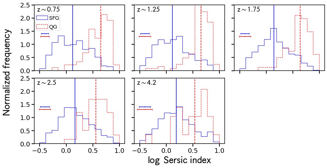
Figure 7: Sérsic index distributions for galaxies in our sample. The distributions of star-forming and quiescent galaxies are shown as blue solid and red dashed histograms, respectively. Median Sérsic indices of star-forming and quiescent galaxies are indicated by the blue solid and red dashed vertical lines, respectively. Quiescent galaxies have larger Sérsic indices on average than star-forming galaxies at all redshifts we consider. Despite the small number of quiescent galaxies in our sample at $z\sim 4.2$, we find that the Sérsic index distributions of star-forming and quiescent galaxies are statistically distinguishable (see text).

6 Discussion

6.1 Comparison with Previous Studies Based on HST Data

We compare our results with previous studies in Figure 6. These studies also examine the evolution with redshift in the rest-frame optical size-mass relation of star-forming galaxies, using only the HST data whereas we use both HST and JWST data. Overall, we find good agreement among our observations and those of other studies where there is overlap in redshift. Small discrepancies between these studies are likely due to differences in sample selection and size as well as differences in methodology.

Evolution with redshift of the intercept, slope, and intrinsic scatter of the size-mass relation for star-forming galaxies are shown in the left, middle, and right panels of the figure, respectively. Our results are presented as black dots with error bars. Results from Table 1 by van der Wel et al. (2014a) are shown as red squares. Intercepts and slopes from Table 2 by Dimauro et al. (2019) are displayed as empty green triangles. These authors did not report uncertainties on their measurements. The results obtained by Mowla et al. (2019) and listed in their Tables 1 and 2 are shown as blue stars in the figure. These authors report the observed scatter in the size-mass relation, which is larger than the intrinsic scatter. Lastly, the results from Table 3 by Nedkova et al. (2021) are presented as magenta diamonds. These authors report the root mean square error (RMSE) instead of an intrinsic scatter for their size-mass relations.

Our measurements of the evolution of the size intercept with redshift agree well with earlier studies up to the highest redshifts examined, as seen in the left panel of Figure 6. In particular, our results are in good agreement with those by Mowla et al. (2019) and Nedkova et al. (2021). Our intercepts are systematically smaller than those measured by van der Wel et al. (2014a) and Dimauro et al. (2019), though these offsets are small, $\lesssim$ 0.05 dex.

At redshifts where these works and ours overlap, our estimates of the slope in the size-mass relation are consistent within errors with those derived by other studies. Our slopes are typically smaller by $\lesssim 0.03$ than those measured by other studies. However, the slopes computed by Dimauro et al. (2019) show a notable deviation from all other studies. Their slopes decrease with increasing redshift, such that they find $\alpha\sim 0.05$ at $z\sim 1.6$. In Section 4.2.1 by Nedkova et al. (2021), the authors discuss extensively why the slopes calculated by Dimauro et al. (2019) decline steeply with redshift, concluding that differences in sample selection between these two studies are the likely cause. We refer the reader to Appendix B by Nedkova et al. (2021) for more details.

At $z\gtrsim 3$, we observe an increase in the slope from $\alpha=0.15$ to $\alpha=0.25$. van der Wel et al. (2014a) and Mowla et al. (2019) observe mild decreases in their slopes at $2<z<3$ and our slope at these redshifts ($\alpha=0.17$) lies in-between theirs. We discuss the potential significance of discovering a higher slope in the size-mass relation at $z\gtrsim 3$ in Section 6.4.

Lastly, the intrinsic scatter in the size-mass relation found here lies between that estimated by other works at overlapping redshifts. Our scatter is nearly constant with redshift, $\sigma\left(\log\ \textrm{R}_{\textrm{eff}}\right)\approx 0.22$. van der Wel et al. (2014a) find scatter that is at most $\sim 0.1$ dex smaller than ours and Nedkova et al. (2021) find RMSE that is consistent with our estimates. As Mowla et al. (2019) only report observed, not intrinsic, scatter, their values are considerably larger than what other studies and our own find. However, their observed scatter fluctuates about a typical value of $\sigma\left(\log\ \textrm{R}_{\textrm{eff}}\right)\sim 0.3$, which is roughly constant with redshift and qualitatively similar to what we find.

Offsets between our estimates and those from previous studies may result from a combination of: different redshift bins; different sample sizes (the samples of van der Wel et al. (2014a) and Dimauro et al. (2019) are approximately 15 and 9 times larger than ours, respectively); different ranges in stellar mass used to measure the size-mass relation; and different methods used to measure rest-frame sizes. Regardless of the causes of these discrepancies, it is reassuring that the same qualitative and similar quantitative evolution in the intercept with redshift is observed when comparing our results with those reported in the literature.

6.2 Comparison with Studies Based on JWST Data

A handful of studies based on JWST data have measured the size-mass relation of star-forming galaxies at redshifts that overlap with those investigated in this paper (Ormerod et al., 2023; Pandya et al., 2023; Sun et al., 2023). However, these studies do not measure all three quantities we use to estimate the size-mass relation (intercept, slope, and scatter) such that direct comparisons between our work and theirs is possible. Therefore, we focus on qualitative comparisons between our results and theirs.

Sun et al. (2023) estimate the size-luminosity relation of 347 galaxies at $4<z<9.5$ in the CEERS survey. These authors use all seven NIRCam bandpasses in CEERS and perform multi-wavelength morphological fits using galfitm, as is done in this work. They infer a slope in the rest-frame optical size-luminosity relation of $0.28\pm 0.04$ at $4<z<9.5$ for the galaxies in their sample with F160W magnitude $<26$; 95% of the galaxies in our sample are brighter than this magnitude limit. It is encouraging that their size-luminosity slope and our size-mass slope at $3<z<5.5$ are consistent within the uncertainties. We can more directly compare our measurements to theirs by computing rest-frame optical luminosities for the subset of our sample at $3<z<5.5$. To do so, we take the apparent magnitudes in F277W and F356W for galaxies at $z<4.2$ and $z>4.2$, respectively, and convert to absolute magnitudes. We find a slope of $\beta=0.31\pm 0.04$ in our size-luminosity relation, which is consistent with the estimates by Sun et al. (2023). At first glance, this comparison would suggest that the slope in the size-mass relation steepens at $z\sim 3$ and stays constant up to $z=9.5$, but additional analysis is needed to confirm this.

Pandya et al. (2023) investigate the distribution of three-dimensional (3D) shapes of star-forming galaxies at $0.5<z<8$ in CEERS. They estimate sizes and axis ratios using both galfit and se++ (Bertin et al., 2020; Kümmel et al., 2022) and statistically infer the distribution of rest-frame optical 3D morphologies as a function of redshift. Consequently, these authors also infer the mean 3D size-mass relation as a function of redshift. While fits to this relation are not presented, they find that the slope of the size-mass relation decreases with increasing redshift. We find that the slope of the size-mass relation is roughly constant up to $z=3$, then steepens slightly at higher redshift. We cannot conclude what exactly causes this discrepancy, but future work should aim to measure both observed 2D and 3D morphologies and compare.

Ormerod et al. (2023) measure the evolution with redshift of galaxy sizes and the size-mass relation in the rest-frame optical for 1,395 galaxies in CEERS. These galaxies are fitted in the NIRCam bandpass that is closest to the rest-frame optical using galfit. Galaxies in their sample are selected to have stellar masses greater than $10^{9.5}\ \textrm{M}_{\odot}$, as is done in this study, but they consider galaxies at $0.5<z\lesssim 8$, whereas our sample is restricted to $0.5<z<5.5$. The stellar masses and redshifts used by Ormerod et al. (2023) come from different sources than what we use, thus it is difficult to explain why our sample contains $\sim 1,000$ more galaxies than theirs despite spanning a smaller range in redshift. With this caveat in mind, we briefly compare our results with theirs. These authors find that galaxy sizes on average decrease with redshift, as we do. However, they consider the evolution with redshift of the average sizes of their sample, instead of that for the intercept in the size-mass relation at a fixed stellar mass, as previous studies and ours have done. Their size-redshift relation (their eq. 5) is consistent with ours to within 2$\sigma$ (see Section 5). Ormerod et al. (2023) find that the sizes of star-forming galaxies increase with stellar mass up to $z\sim 6$, though they do not report fitting these relations. Their size-mass relations may be affected by how they separate star-forming and quiescent galaxies. They use the midpoint of the specific star-formation rate distribution in each of their redshift bins to distinguish these populations, whereas we use rest-frame optical colors to do so. A proper comparison of our work with that by Ormerod et al. (2023) would necessitate reconstructing their sample, which is beyond the scope of this work.

6.3 Comparisons with Simulations

We now compare our measurements of the size-mass relation as a function of redshift with predictions from simulations. At $z\lesssim 3$, where our sample overlaps with prior HST-based studies, large cosmological hydrodynamical simulations, such as EAGLE (Schaye et al., 2015; Crain et al., 2015) and IllustrisTNG (Marinacci et al., 2018; Naiman et al., 2018; Nelson et al., 2018; Pillepich et al., 2018; Springel et al., 2018), are in good agreement with observations (Furlong et al., 2017; Genel et al., 2018). In particular, Furlong et al. (2017) report normalizations in their size-mass relations that are within 0.1 dex of those estimated by van der Wel et al. (2014a) from $z\sim 0$ to $z=2$, and Genel et al. (2018) report a slope in the size-mass relation of their star-forming galaxies at $z=2$ that is approximately 0.15. These findings agree well with our results: we find sizes that are also within 0.1 dex of those measured by van der Wel et al. (2014a) out to $z=3$, and our slope $\alpha\approx 0.16$ at $z\sim 2$ is consistent with what Genel et al. (2018) find (see Table 1).

At higher redshifts, $z>3$, there is tension between our results and those seen in simulations. Costantin et al. (2023) examine how galaxy sizes and the size-mass relation evolve from $z=3$ to $z=6$ in the TNG50 simulation. To do so, these authors produce mock images of their simulated galaxies and include the effects of radiative transfer due to dust and instrumental effects resulting from observing with JWST. Morphologies are then measured in these mock images and two sets of measurements are presented: one that is intrinsic to the simulation and based on 3D half-mass radii, and one that is based on their mock images. We compare the latter with our results.

Costantin et al. (2023) find that the sizes of star-forming galaxies decrease with redshift, as we do, though we find larger sizes at fixed stellar mass. At the stellar mass that corresponds to the intercept of our fits to the size-mass relation, $\log\textrm{M}_{\star}=10^{10.7}\ \textrm{M}_{\odot}$, we find a typical size of $10^{0.41}$ kpc at $z\sim 4.2$, whereas Costantin et al. (2023) find a typical size of $10^{0.15}$ kpc at $z=4$. Costantin et al. (2023) also find that the slope of the size-mass relation for star-forming galaxies decreases with increasing redshift. At $z=3$ and $z=4$, these authors measure slopes between $a_{\textrm{obs}}=0.05$ and $a_{\textrm{obs}}=0.11$ in the F200W and F356W bandpasses. At $z>5$, they find slopes that are negative. At $3<z<5.5$, we find that the slope is $0.25^{+0.05}_{-0.03}$, which is in significant disagreement with the TNG50 simulations. Negative slopes in the size-mass relation at $z\gtrsim 5$ have been reported in other simulations, such as BLUETIDES (Feng et al., 2016; Marshall et al., 2022) and FLARES (Lovell et al., 2021; Roper et al., 2022). Costantin et al. (2023) note that the discrepancy between simulated and observed size-mass relations may be attributed to shortcomings in modeling the complex morphologies of high-redshift galaxies when using only one-component Sérsic models as well as dust obscuration (see also Roper et al. 2022).

6.4 Implications Regarding the Evolution of Star-forming Galaxies

Models of disk galaxy formation and evolution often assume proportional relationships between the properties of dark matter halos and those of the galaxies they host (e.g., Fall & Efstathiou, 1980; Mo et al., 1998). These proportional relations arise as gas in galaxies is expected to inherit the specific angular momentum from the host dark matter halo. We briefly discuss how our results fit into this paradigm below.

The intrinsic scatter in our measured size-mass relation is nearly constant at $\sigma\left(\log\ \textrm{R}_{\textrm{eff}}\right)\approx 0.22$ from $z\sim 0.7$ to $z\sim 4.2$. This value is strikingly similar to the predicted scatter of 0.25 dex (in log base 10) in the halo spin parameter (e.g., Bullock et al., 2001; Macciò et al., 2008). This finding suggests that the sizes of galaxies are set by the sizes of their dark matter halos since $z=5.5$. We consider the connection between galaxy and dark matter halo properties further.

We find that the slope in the size-mass relation is approximately constant at $\alpha\approx 0.16$ up to $z\sim 3$ and increases slightly to $\alpha=0.25$ at higher redshift. Shen et al. (2003) argue that if the ratio of galaxy mass to halo mass were constant, the observed slope would be steeper, $\alpha=1/3$. This argument assumes that galaxy sizes are proportional to halo sizes. At $0<z<3$, disk galaxies are indeed observed to have sizes that are proportional to those of their halos (Kravtsov, 2013; Huang et al., 2017). Assuming this relation at $z\sim 4.2$, we use Equation 23 by Shen et al. (2003) to derive the stellar mass-halo mass relation, finding $\textrm{M}_{\star}/\textrm{M}_{h}\propto M_{h}^{1/(3\alpha)-1}$. From our results, this suggests that $\textrm{M}_{\star}/\textrm{M}_{h}\propto M_{h}^{\gamma\sim 1}$ at $z\lesssim 3$ and $\textrm{M}_{\star}/\textrm{M}_{h}\propto M_{h}^{\gamma\sim 0.3}$ at $z\gtrsim 3$. Our inferred slopes in the stellar mass - halo mass relation are consistent with measurements thereof at $z<3$ for lower halo masses (Behroozi et al., 2013; Moster et al., 2013; Girelli et al., 2020).

The results we have discussed thus far imply that star-forming galaxies on average at $0.5<z<5.5$ inherit the specific angular momenta of their host DM halos. This suggests that the stellar kinematics of these galaxies may resemble what is expected of rotating disks. However, a number of studies find that high-redshift galaxies are likely not rotating, oblate disks, but rather prolate, cigar-shaped systems (van der Wel et al., 2014b; Zhang et al., 2019; Pandya et al., 2023). These findings are also supported by simulations (Tomassetti et al., 2016; Vega-Ferrero et al., 2023). While the results from these studies may complicate the interpretation of our results above, the possibility that high-redshift galaxies are predominantly prolate may explain why we observe a steeper size-mass slope at $z>3$ than at lower redshifts.

A steeper slope in the size-mass relation with respect to redshift may arise due to either A) low-mass galaxies decreasing in size with redshift faster than high-mass galaxies, or B) high-mass galaxies increasing in size with redshift faster than low-mass galaxies. As can be seen in Figure 6, sizes at $\textrm{M}_{\star}=5\times 10^{10}\ \textrm{M}_{\odot}$ decrease with redshift, hence the latter explanation above is unlikely. Pandya et al. (2023) find that low-mass galaxies are most likely prolate at high redshift, with prolate fractions of $\sim 80\%$ at $3<z<8$. The transition from oblate disks at low redshift to prolate systems at high redshift may be accompanied by transitions in the sizes of such galaxies from large to small.

7 Conclusions

We use the early release JWST data taken by the CEERS survey, in combination with available HST data, to examine the size-mass relation of star-forming galaxies and compare the morphologies of star-forming and quiescent galaxies in the rest-frame optical at $0.5<z<5.5$. We fit the sizes of 2,450 galaxies across 13 bandpasses and derive sizes and Sérsic indices in the rest-frame 5,000Å using a simultaneous multi-wavelength fitting approach.

The main conclusions we find from our investigation of the mass-size relation are summarized as follows:

1. The slope of the size-mass relation ($\textrm{d}\log\textrm{R}_{\textrm{eff}}\ /\ \textrm{d}\log\textrm{M}_{\star}$) appears to be constant out to $z\lesssim 3$ and steepens slightly at $z\gtrsim 3$ (middle panel in Figure 6). Our measurements are consistent with previous work out to $z\sim 3$ as well as some studies at higher redshifts than what is considered here.

2. The intercept of the size-mass relation ($\log(A)$) continues to decline at a rate similar to what other studies find out to $z=5.5$ (left panel of Figure 6). Our measurements agree well with those in the literature at lower redshifts and are consistent despite our smaller sample size by a factor of at least 9.

3. The scatter of the size-mass relation ($\sigma\left(\log\ \textrm{R}_{\textrm{eff}}\right)$) is roughly constant out to $z=5.5$ (right panel in Figure 6). This suggests a tight connection between the properties of star-forming galaxies and their dark matter halos, which may suggest the prevalence of disk galaxies at high redshift. However, our observations of the evolution of the slope with redshift may also be consistent with the occurrence of prolate galaxies at similar redshifts.

4. Star-forming and quiescent galaxies have clearly separate distributions in Sérsic index. Star-forming and quiescent galaxies have typical Sérsic indices $n\sim 1.3$ and $n\sim 4.3$, respectively, at all redshifts we consider.

This pilot study of galaxy morphologies at high redshift, with the unparalleled combination of JWST and HST data, extends the characterization of the size-mass relation of star-forming galaxies and the morphology-quenching relation at high stellar mass out to $z=5.5$. Future work would benefit from combining data from CEERS with other large JWST surveys, such as COSMOS-Web (Casey et al., 2022) and UNCOVER (Bezanson et al., 2022).

8 Acknowledgements

Appendix A Comparison to Single-Band Measurements Using GALFIT

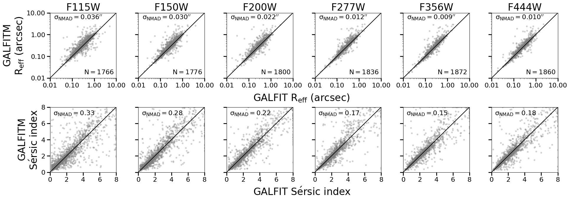
Figure 8: Comparison of the sizes (top row) and the Sérsic indices (bottom row) between galfit and galfitm. We select $\sim 1,800$ galaxies in our sample that have satisfactory galfit fits (as discussed in the text). The number of galaxies that meet these fit criteria in each bandpass is listed in the lower right corner in each panel in the top row. Overall, there is good agreement between the two sets of measurements, as quantified by the NMAD scatter, which is displayed in the top left corner of each panel. The scatter is wavelength dependent: it is largest in F115W (left columns) and smallest at longer wavelengths (rightmost columns), though it is generally small: $\sigma_{\textrm{NMAD}}\sim 0.02$ arcsec in size and $\sigma_{\textrm{NMAD}}\sim 0.2$ in Sérsic index.

In Figure 8, we compare effective radii and Sérsic indices from galfit measurements by McGrath et al. (in prep.) with our measurements using galfitm in six NIRCam bandpasses in the top and bottom rows, respectively. We compare these measurements for $\sim 1,800$ galaxies in our sample that are selected to have galfit flag values equal to zero in each bandpass. A flag value equal to zero denotes fits that satisfy the following: the galfit-estimated magnitudes are consistent with those estimatd by Source Extractor; all parameters lie within their respective constraints; galfit found best-fitting solutions; and the objects are located far from the edge of the detector. In the galfit fits, the position angle and axis ratio are left to vary freely in each bandpass independently, whereas in our galfitm fits, these two parameters are fixed to the same values in all bandpasses.

There is good agreement in general between our galfitm measurements and those performed using galfit. Most galaxies, shown as gray dots in the figure, lie on or near the the one-to-one line, displayed as a black line. To quantify the scatter between the two sets of estimates, we use the NMAD, mentioned previously in Section 2.2, which is shown in the top left corner of each panel. Effective radii agree well, and the $\sigma_{\textrm{NMAD}}\sim 0.02$ arcsec, though this depends on wavelength: the scatter is about four times larger in F115W than in F444W, though the scatter is at most 1.2 pixels. For the Sérsic indices, we also find good agreement: the typical $\sigma_{\textrm{NMAD}}\sim 0.2$. This scatter also depends on wavelength, with the scatter in F115W about twice that in F444W.

References

- Abramowitz & Stegun (1965) Abramowitz, M., & Stegun, I. A. 1965, Handbook of mathematical functions with formulas, graphs, and mathematical tables
- Astropy Collaboration et al. (2013) Astropy Collaboration, Robitaille, T. P., Tollerud, E. J., et al. 2013, A&A, 558, A33, doi: 10.1051/0004-6361/201322068
- Astropy Collaboration et al. (2018) Astropy Collaboration, Price-Whelan, A. M., Sipőcz, B. M., et al. 2018, AJ, 156, 123, doi: 10.3847/1538-3881/aabc4f
- Bagley et al. (2023) Bagley, M. B., Finkelstein, S. L., Koekemoer, A. M., et al. 2023, ApJ, 946, L12, doi: 10.3847/2041-8213/acbb08
- Baldry et al. (2006) Baldry, I. K., Balogh, M. L., Bower, R. G., et al. 2006, MNRAS, 373, 469, doi: 10.1111/j.1365-2966.2006.11081.x
- Barden et al. (2012) Barden, M., Häußler, B., Peng, C. Y., McIntosh, D. H., & Guo, Y. 2012, MNRAS, 422, 449, doi: 10.1111/j.1365-2966.2012.20619.x
- Barro et al. (2023) Barro, G., Perez-Gonzalez, P. G., Kocevski, D. D., et al. 2023, arXiv e-prints, arXiv:2305.14418, doi: 10.48550/arXiv.2305.14418
- Behroozi et al. (2013) Behroozi, P. S., Wechsler, R. H., & Conroy, C. 2013, ApJ, 770, 57, doi: 10.1088/0004-637X/770/1/57
- Bertin et al. (2020) Bertin, E., Schefer, M., Apostolakos, N., et al. 2020, in Astronomical Society of the Pacific Conference Series, Vol. 527, Astronomical Data Analysis Software and Systems XXIX, ed. R. Pizzo, E. R. Deul, J. D. Mol, J. de Plaa, & H. Verkouter, 461
- Bezanson et al. (2009) Bezanson, R., van Dokkum, P. G., Tal, T., et al. 2009, ApJ, 697, 1290, doi: 10.1088/0004-637X/697/2/1290
- Bezanson et al. (2022) Bezanson, R., Labbe, I., Whitaker, K. E., et al. 2022, arXiv e-prints, arXiv:2212.04026, doi: 10.48550/arXiv.2212.04026
- Bradley et al. (2022) Bradley, L., Sipőcz, B., Robitaille, T., et al. 2022, astropy/photutils: 1.5.0, 1.5.0, Zenodo, doi: 10.5281/zenodo.6825092
- Brammer et al. (2008) Brammer, G. B., van Dokkum, P. G., & Coppi, P. 2008, ApJ, 686, 1503, doi: 10.1086/591786
- Bruce et al. (2012) Bruce, V. A., Dunlop, J. S., Cirasuolo, M., et al. 2012, MNRAS, 427, 1666, doi: 10.1111/j.1365-2966.2012.22087.x
- Bruzual & Charlot (2003) Bruzual, G., & Charlot, S. 2003, MNRAS, 344, 1000, doi: 10.1046/j.1365-8711.2003.06897.x
- Buitrago et al. (2008) Buitrago, F., Trujillo, I., Conselice, C. J., et al. 2008, ApJ, 687, L61, doi: 10.1086/592836
- Bullock et al. (2001) Bullock, J. S., Dekel, A., Kolatt, T. S., et al. 2001, ApJ, 555, 240, doi: 10.1086/321477
- Calzetti et al. (2000) Calzetti, D., Armus, L., Bohlin, R. C., et al. 2000, ApJ, 533, 682, doi: 10.1086/308692
- Carollo et al. (2013) Carollo, C. M., Bschorr, T. J., Renzini, A., et al. 2013, ApJ, 773, 112, doi: 10.1088/0004-637X/773/2/112
- Casey et al. (2022) Casey, C. M., Kartaltepe, J. S., Drakos, N. E., et al. 2022, arXiv e-prints, arXiv:2211.07865, doi: 10.48550/arXiv.2211.07865
- Chabrier (2003) Chabrier, G. 2003, PASP, 115, 763, doi: 10.1086/376392
- Conroy & Gunn (2010) Conroy, C., & Gunn, J. E. 2010, ApJ, 712, 833, doi: 10.1088/0004-637X/712/2/833
- Conselice et al. (2011) Conselice, C. J., Bluck, A. F. L., Buitrago, F., et al. 2011, MNRAS, 413, 80, doi: 10.1111/j.1365-2966.2010.18113.x
- Costantin et al. (2023) Costantin, L., Pérez-González, P. G., Vega-Ferrero, J., et al. 2023, ApJ, 946, 71, doi: 10.3847/1538-4357/acb926
- Crain et al. (2015) Crain, R. A., Schaye, J., Bower, R. G., et al. 2015, MNRAS, 450, 1937, doi: 10.1093/mnras/stv725
- Dahlen et al. (2013) Dahlen, T., Mobasher, B., Faber, S. M., et al. 2013, ApJ, 775, 93, doi: 10.1088/0004-637X/775/2/93
- Davidzon et al. (2017) Davidzon, I., Ilbert, O., Laigle, C., et al. 2017, A&A, 605, A70, doi: 10.1051/0004-6361/201730419
- Davis et al. (2007) Davis, M., Guhathakurta, P., Konidaris, N. P., et al. 2007, ApJ, 660, L1, doi: 10.1086/517931
- Dimauro et al. (2019) Dimauro, P., Huertas-Company, M., Daddi, E., et al. 2019, MNRAS, 489, 4135, doi: 10.1093/mnras/stz2421
- Dutton et al. (2007) Dutton, A. A., van den Bosch, F. C., Dekel, A., & Courteau, S. 2007, ApJ, 654, 27, doi: 10.1086/509314
- El-Badry et al. (2016) El-Badry, K., Wetzel, A., Geha, M., et al. 2016, ApJ, 820, 131, doi: 10.3847/0004-637X/820/2/131
- Faisst et al. (2017) Faisst, A. L., Carollo, C. M., Capak, P. L., et al. 2017, ApJ, 839, 71, doi: 10.3847/1538-4357/aa697a
- Fall & Efstathiou (1980) Fall, S. M., & Efstathiou, G. 1980, MNRAS, 193, 189, doi: 10.1093/mnras/193.2.189
- Feng et al. (2016) Feng, Y., Di-Matteo, T., Croft, R. A., et al. 2016, MNRAS, 455, 2778, doi: 10.1093/mnras/stv2484
- Ferguson et al. (2004) Ferguson, H. C., Dickinson, M., Giavalisco, M., et al. 2004, ApJ, 600, L107, doi: 10.1086/378578
- Ferreira et al. (2023) Ferreira, L., Conselice, C. J., Sazonova, E., et al. 2023, ApJ, 955, 94, doi: 10.3847/1538-4357/acec76
- Finkelstein et al. (2022) Finkelstein, S. L., Bagley, M. B., Haro, P. A., et al. 2022, ApJ, 940, L55, doi: 10.3847/2041-8213/ac966e
- Finkelstein et al. (2023) Finkelstein, S. L., Bagley, M. B., Ferguson, H. C., et al. 2023, ApJ, 946, L13, doi: 10.3847/2041-8213/acade4
- Foreman-Mackey et al. (2013) Foreman-Mackey, D., Hogg, D. W., Lang, D., & Goodman, J. 2013, PASP, 125, 306, doi: 10.1086/670067
- Furlong et al. (2017) Furlong, M., Bower, R. G., Crain, R. A., et al. 2017, MNRAS, 465, 722, doi: 10.1093/mnras/stw2740
- Gaia Collaboration et al. (2021) Gaia Collaboration, Brown, A. G. A., Vallenari, A., et al. 2021, A&A, 649, A1, doi: 10.1051/0004-6361/202039657
- Genel et al. (2018) Genel, S., Nelson, D., Pillepich, A., et al. 2018, MNRAS, 474, 3976, doi: 10.1093/mnras/stx3078
- Girelli et al. (2020) Girelli, G., Pozzetti, L., Bolzonella, M., et al. 2020, A&A, 634, A135, doi: 10.1051/0004-6361/201936329
- Grogin et al. (2011) Grogin, N. A., Kocevski, D. D., Faber, S. M., et al. 2011, ApJS, 197, 35, doi: 10.1088/0067-0049/197/2/35
- Guo et al. (2023) Guo, Y., Jogee, S., Finkelstein, S. L., et al. 2023, ApJ, 945, L10, doi: 10.3847/2041-8213/acacfb
- Harris et al. (2020) Harris, C. R., Millman, K. J., van der Walt, S. J., et al. 2020, Nature, 585, 357, doi: 10.1038/s41586-020-2649-2
- Häußler et al. (2013) Häußler, B., Bamford, S. P., Vika, M., et al. 2013, MNRAS, 430, 330, doi: 10.1093/mnras/sts633
- Häußler et al. (2022) Häußler, B., Vika, M., Bamford, S. P., et al. 2022, A&A, 664, A92, doi: 10.1051/0004-6361/202142935
- Holwerda et al. (2015) Holwerda, B. W., Bouwens, R., Oesch, P., et al. 2015, ApJ, 808, 6, doi: 10.1088/0004-637X/808/1/6
- Holwerda et al. (2023) Holwerda, B. W., Hsu, C.-C., Hathi, N., et al. 2023, arXiv e-prints, arXiv:2309.05835, doi: 10.48550/arXiv.2309.05835
- Hoyos et al. (2011) Hoyos, C., den Brok, M., Verdoes Kleijn, G., et al. 2011, MNRAS, 411, 2439, doi: 10.1111/j.1365-2966.2010.17855.x
- Hoyos et al. (2012) Hoyos, C., Aragón-Salamanca, A., Gray, M. E., et al. 2012, MNRAS, 419, 2703, doi: 10.1111/j.1365-2966.2011.19918.x
- Huang et al. (2017) Huang, K.-H., Fall, S. M., Ferguson, H. C., et al. 2017, ApJ, 838, 6, doi: 10.3847/1538-4357/aa62a6
- Huertas-Company et al. (2023) Huertas-Company, M., Iyer, K. G., Angeloudi, E., et al. 2023, arXiv e-prints, arXiv:2305.02478, doi: 10.48550/arXiv.2305.02478
- Hunter (2007) Hunter, J. D. 2007, Computing in Science & Engineering, 9, 90, doi: 10.1109/MCSE.2007.55
- Kartaltepe et al. (2023) Kartaltepe, J. S., Rose, C., Vanderhoof, B. N., et al. 2023, ApJ, 946, L15, doi: 10.3847/2041-8213/acad01
- Kauffmann et al. (2003) Kauffmann, G., Heckman, T. M., White, S. D. M., et al. 2003, MNRAS, 341, 33, doi: 10.1046/j.1365-8711.2003.06291.x
- Koekemoer et al. (2011) Koekemoer, A. M., Faber, S. M., Ferguson, H. C., et al. 2011, ApJS, 197, 36, doi: 10.1088/0067-0049/197/2/36
- Kormendy & Bender (1996) Kormendy, J., & Bender, R. 1996, ApJ, 464, L119, doi: 10.1086/310095
- Kravtsov (2013) Kravtsov, A. V. 2013, ApJ, 764, L31, doi: 10.1088/2041-8205/764/2/L31
- Kriek et al. (2009) Kriek, M., van Dokkum, P. G., Labbé, I., et al. 2009, ApJ, 700, 221, doi: 10.1088/0004-637X/700/1/221
- Kümmel et al. (2022) Kümmel, M., Álvarez-Ayllón, A., Bertin, E., et al. 2022, arXiv e-prints, arXiv:2212.02428, doi: 10.48550/arXiv.2212.02428
- Labbé et al. (2023) Labbé, I., van Dokkum, P., Nelson, E., et al. 2023, Nature, 616, 266, doi: 10.1038/s41586-023-05786-2
- Lang et al. (2014) Lang, P., Wuyts, S., Somerville, R. S., et al. 2014, ApJ, 788, 11, doi: 10.1088/0004-637X/788/1/11
- Lange et al. (2015) Lange, R., Driver, S. P., Robotham, A. S. G., et al. 2015, MNRAS, 447, 2603, doi: 10.1093/mnras/stu2467
- Long et al. (2023) Long, A. S., Antwi-Danso, J., Lambrides, E. L., et al. 2023, arXiv e-prints, arXiv:2305.04662, doi: 10.48550/arXiv.2305.04662
- Lovell et al. (2021) Lovell, C. C., Vijayan, A. P., Thomas, P. A., et al. 2021, MNRAS, 500, 2127, doi: 10.1093/mnras/staa3360
- Macciò et al. (2008) Macciò, A. V., Dutton, A. A., & van den Bosch, F. C. 2008, MNRAS, 391, 1940, doi: 10.1111/j.1365-2966.2008.14029.x
- Margalef-Bentabol et al. (2016) Margalef-Bentabol, B., Conselice, C. J., Mortlock, A., et al. 2016, MNRAS, 461, 2728, doi: 10.1093/mnras/stw1451
- Marinacci et al. (2018) Marinacci, F., Vogelsberger, M., Pakmor, R., et al. 2018, MNRAS, 480, 5113, doi: 10.1093/mnras/sty2206
- Marshall et al. (2022) Marshall, M. A., Wilkins, S., Di Matteo, T., et al. 2022, MNRAS, 511, 5475, doi: 10.1093/mnras/stac380
- Martorano et al. (2023) Martorano, M., van der Wel, A., Bell, E. F., et al. 2023, Rest-Frame Near-Infrared Radial Light Profiles up to z=3 from JWST/NIRCam: Wavelength Dependence of the Sérsic Index. https://arxiv.org/abs/2308.11392
- Matthee et al. (2023) Matthee, J., Naidu, R. P., Brammer, G., et al. 2023, arXiv e-prints, arXiv:2306.05448, doi: 10.48550/arXiv.2306.05448
- Mo et al. (1998) Mo, H. J., Mao, S., & White, S. D. M. 1998, MNRAS, 295, 319, doi: 10.1046/j.1365-8711.1998.01227.x
- Mosleh et al. (2012) Mosleh, M., Williams, R. J., Franx, M., et al. 2012, ApJ, 756, L12, doi: 10.1088/2041-8205/756/1/L12
- Moster et al. (2013) Moster, B. P., Naab, T., & White, S. D. M. 2013, MNRAS, 428, 3121, doi: 10.1093/mnras/sts261
- Mowla et al. (2019) Mowla, L. A., van Dokkum, P., Brammer, G. B., et al. 2019, ApJ, 880, 57, doi: 10.3847/1538-4357/ab290a
- Naab et al. (2009) Naab, T., Johansson, P. H., & Ostriker, J. P. 2009, ApJ, 699, L178, doi: 10.1088/0004-637X/699/2/L178
- Naiman et al. (2018) Naiman, J. P., Pillepich, A., Springel, V., et al. 2018, MNRAS, 477, 1206, doi: 10.1093/mnras/sty618
- Nandra et al. (2015) Nandra, K., Laird, E. S., Aird, J. A., et al. 2015, ApJS, 220, 10, doi: 10.1088/0067-0049/220/1/10
- Nedkova et al. (2021) Nedkova, K. V., Häußler, B., Marchesini, D., et al. 2021, MNRAS, 506, 928, doi: 10.1093/mnras/stab1744
- Nelson et al. (2018) Nelson, D., Pillepich, A., Springel, V., et al. 2018, MNRAS, 475, 624, doi: 10.1093/mnras/stx3040
- Newville et al. (2014) Newville, M., Stensitzki, T., Allen, D. B., & Ingargiola, A. 2014, LMFIT: Non-Linear Least-Square Minimization and Curve-Fitting for Python, 0.8.0, Zenodo, Zenodo, doi: 10.5281/zenodo.11813
- Oesch et al. (2010) Oesch, P. A., Bouwens, R. J., Carollo, C. M., et al. 2010, ApJ, 709, L21, doi: 10.1088/2041-8205/709/1/L21
- Oke & Gunn (1983) Oke, J. B., & Gunn, J. E. 1983, ApJ, 266, 713, doi: 10.1086/160817
- Ono et al. (2013) Ono, Y., Ouchi, M., Curtis-Lake, E., et al. 2013, ApJ, 777, 155, doi: 10.1088/0004-637X/777/2/155
- Ormerod et al. (2023) Ormerod, K., Conselice, C. J., Adams, N. J., et al. 2023, arXiv e-prints, arXiv:2309.04377, doi: 10.48550/arXiv.2309.04377
- Pandya et al. (2023) Pandya, V., Zhang, H., Huertas-Company, M., et al. 2023, arXiv e-prints, arXiv:2310.15232. https://arxiv.org/abs/2310.15232
- Peng et al. (2002) Peng, C. Y., Ho, L. C., Impey, C. D., & Rix, H.-W. 2002, AJ, 124, 266, doi: 10.1086/340952
- Peng et al. (2010) —. 2010, AJ, 139, 2097, doi: 10.1088/0004-6256/139/6/2097
- Perrin et al. (2014) Perrin, M. D., Sivaramakrishnan, A., Lajoie, C.-P., et al. 2014, in Society of Photo-Optical Instrumentation Engineers (SPIE) Conference Series, Vol. 9143, Space Telescopes and Instrumentation 2014: Optical, Infrared, and Millimeter Wave, ed. J. Oschmann, Jacobus M., M. Clampin, G. G. Fazio, & H. A. MacEwen, 91433X, doi: 10.1117/12.2056689
- Pillepich et al. (2018) Pillepich, A., Nelson, D., Hernquist, L., et al. 2018, MNRAS, 475, 648, doi: 10.1093/mnras/stx3112
- Robertson et al. (2006) Robertson, B., Bullock, J. S., Cox, T. J., et al. 2006, ApJ, 645, 986, doi: 10.1086/504412
- Roper et al. (2022) Roper, W. J., Lovell, C. C., Vijayan, A. P., et al. 2022, MNRAS, 514, 1921, doi: 10.1093/mnras/stac1368
- Schaye et al. (2015) Schaye, J., Crain, R. A., Bower, R. G., et al. 2015, MNRAS, 446, 521, doi: 10.1093/mnras/stu2058
- Sersic (1968) Sersic, J. L. 1968, Atlas de Galaxias Australes
- Shen et al. (2003) Shen, S., Mo, H. J., White, S. D. M., et al. 2003, MNRAS, 343, 978, doi: 10.1046/j.1365-8711.2003.06740.x
- Shibuya et al. (2015) Shibuya, T., Ouchi, M., & Harikane, Y. 2015, ApJS, 219, 15, doi: 10.1088/0067-0049/219/2/15
- Skelton et al. (2014) Skelton, R. E., Whitaker, K. E., Momcheva, I. G., et al. 2014, ApJS, 214, 24, doi: 10.1088/0067-0049/214/2/24
- Springel et al. (2018) Springel, V., Pakmor, R., Pillepich, A., et al. 2018, MNRAS, 475, 676, doi: 10.1093/mnras/stx3304
- Stefanon et al. (2017) Stefanon, M., Yan, H., Mobasher, B., et al. 2017, ApJS, 229, 32, doi: 10.3847/1538-4365/aa66cb
- Suess et al. (2022) Suess, K. A., Bezanson, R., Nelson, E. J., et al. 2022, ApJ, 937, L33, doi: 10.3847/2041-8213/ac8e06
- Sun et al. (2023) Sun, W., Ho, L. C., Zhuang, M.-Y., et al. 2023, arXiv e-prints, arXiv:2308.09076, doi: 10.48550/arXiv.2308.09076
- Tomassetti et al. (2016) Tomassetti, M., Dekel, A., Mandelker, N., et al. 2016, MNRAS, 458, 4477, doi: 10.1093/mnras/stw606
- Trujillo et al. (2006) Trujillo, I., Förster Schreiber, N. M., Rudnick, G., et al. 2006, ApJ, 650, 18, doi: 10.1086/506464
- van der Wel et al. (2012) van der Wel, A., Bell, E. F., Häussler, B., et al. 2012, ApJS, 203, 24, doi: 10.1088/0067-0049/203/2/24
- van der Wel et al. (2014a) van der Wel, A., Franx, M., van Dokkum, P. G., et al. 2014a, ApJ, 788, 28, doi: 10.1088/0004-637X/788/1/28
- van der Wel et al. (2014b) van der Wel, A., Chang, Y.-Y., Bell, E. F., et al. 2014b, ApJ, 792, L6, doi: 10.1088/2041-8205/792/1/L6
- Vega-Ferrero et al. (2023) Vega-Ferrero, J., Huertas-Company, M., Costantin, L., et al. 2023, arXiv e-prints, arXiv:2302.07277, doi: 10.48550/arXiv.2302.07277
- Vika et al. (2013) Vika, M., Bamford, S. P., Häußler, B., et al. 2013, MNRAS, 435, 623, doi: 10.1093/mnras/stt1320
- Virtanen et al. (2020) Virtanen, P., Gommers, R., Oliphant, T. E., et al. 2020, Nature Methods, 17, 261, doi: 10.1038/s41592-019-0686-2
- Vulcani et al. (2014) Vulcani, B., Bamford, S. P., Häußler, B., et al. 2014, MNRAS, 441, 1340, doi: 10.1093/mnras/stu632
- Whitaker et al. (2011) Whitaker, K. E., Labbé, I., van Dokkum, P. G., et al. 2011, ApJ, 735, 86, doi: 10.1088/0004-637X/735/2/86
- Williams et al. (2009) Williams, R. J., Quadri, R. F., Franx, M., van Dokkum, P., & Labbé, I. 2009, ApJ, 691, 1879, doi: 10.1088/0004-637X/691/2/1879
- Wuyts et al. (2011) Wuyts, S., Förster Schreiber, N. M., van der Wel, A., et al. 2011, ApJ, 742, 96, doi: 10.1088/0004-637X/742/2/96
- Zhang et al. (2019) Zhang, H., Primack, J. R., Faber, S. M., et al. 2019, MNRAS, 484, 5170, doi: 10.1093/mnras/stz339