Parity violation in gravitational waves and observational bounds from third-generation detectors

Abstract

In this paper, we analyze parity-violating effects in the propagation of gravitational waves (GWs). For this purpose, we adopt a newly proposed parametrized post-Einstenian (PPE) formalism, which encodes modified gravity corrections to the phase and amplitude of GW waveforms. In particular, we focus our study on three well-known examples of parity-violating theories, namely Chern-Simons, Symmetric Teleparallel and Horǎva-Lishitz gravity. For each model, we identify the PPE parameters emerging from the inclusion of parity-violating terms in the gravitational Lagrangian. Thus, we use the simulated sensitivities of third-generation GW interferometers, such as the Einstein Telescope and Cosmic Explorer, to obtain numerical bounds on the PPE coefficients and the physical parameters of binary systems. In so doing, we find that deviations from General Relativity cannot be excluded within given confidence limits. Moreover, our results show an improvement of one order of magnitude in the relative accuracy of the GW parameters compared to the values inferred from the LIGO-Virgo-KAGRA network. In this respect, the present work demonstrates the power of next-generation GW detectors to probe fundamental physics with unprecedented precision.

I Introduction

The gravitational wave (GW) observations by binary black holes (BBH) and/or binary neutron stars (BNS) detected by the LIGO-Virgo-KAGRA (LVK) collaboration [1, 2, 3] have opened a new window to investigate fundamental physics. In this respect, the degeneracy among different theoretical scenarios brings attention to the need for investigating astrophysical sources via direct manifestations of gravitational effects. This could yield valuable physical information on the nature of gravity itself, thus playing a significant role in probing extra degrees of freedom with respect to General Relativity (GR) [4, 5, 6, 7, 8, 9]. On the other hand, the dark energy issue related to the standard cosmological model further motivated, in the last years, the search for possible extensions or modifications of GR [10, 11, 12, 13, 14, 15, 16, 17]. The latter typically emerge from high-energy theories and can lead to small departures from GR in the infrared limit [18, 19, 20, 21, 22, 23, 24, 25].

Different impacts of modified theories of gravity on GWs can be ascribed to changes in the amplitude and/or the phase of the GW signal propagation. Changes in the phase (amplitude) may occur due to modifications of the real (imaginary) part of the dispersion relations of GWs [26, 27, 28, 29]. An example of the broad class of modified gravity scenarios sharing similar consequences is represented by gravitational actions that are not invariant under a parity transformation. Parity-violating theories are characterized by an asymmetry in the propagation amplitude and speed of the left and right-handed GW polarization modes, leading to amplitude and phase birefringence, respectively [30, 31, 32, 33, 34].

A well-known example of a parity-violating gravity scenario is the Chern-Simons (CS) theory [35, 36, 37, 38, 39], in which the Einstein-Hilbert action is extended to contain a dynamical scalar field coupled to the CS term. The parity-violating effect is due to the coupling between the (even parity) cosmological scalar field and the (odd parity) Pontryagin invariant. CS gravity takes inspiration from string theory [40] and represents the only case of a metric theory, quadratic in the curvature and linear in the scalar field, violating parity. Moreover, the CS theory can be obtained as a limit case of the more general class of ghost-free scalar-tensor gravity [41, 31, 42], which includes parity-violating terms arising from higher-order derivatives of the scalar field.

Additional relevant examples of parity-violating theories include Symmetric Teleparallel (ST) gravity [43, 44, 45], which is built upon the non-metricity tensor, and some versions of Hořava-Lifshitz (HL) gravity [46]. First introduced as a renormalizable extension of GR, HL gravity breaks Lorentz invariance and contains higher-order derivative operators that induce parity violation [47].

A widely adopted framework to explore deviations from GR in GW propagation is provided by the parametrized post-Einstenian (PPE) formalism [48]. Similarly to the post-Newtonian scheme, the PPE formalism encodes modified gravity corrections to the phase and amplitude of GR waveforms [49, 50, 51]. Thus, the PPE formalism can reveal a useful tool to probe GR through GW data. Several non-PPE analyses of GW data to search for possible parity violations were previously performed only for particular waveform parametrizations [52, 53, 54]. In fact, the first full PPE study of parity-violating theories has been recently presented in Ref. [34], where a model-independent framework was introduced to parametrize parity-violating effects in the GW-modified gravity propagation under a general scheme.

In light of the theoretical results found in Ref. [34], we intend to apply the PPE framework to future GW simulated observations, in order to obtain forecast bounds on gravitational parity violation. For this purpose, we employ in our analysis the experimental sensitivities of the third-generation (3G) GW detectors, such as the Einstein Telescope (ET) [55, 56] and Cosmic Explorer (CE) [57, 58] interferometers. The latter have been extensively used, in recent years, to investigate scenarios beyond GR, the dark energy problem and many other fundamental questions in gravitational physics [59, 60, 61, 62, 63, 64, 65, 66, 67, 68, 69, 70, 71, 72].

The structure of the paper is as follows. In Sec. II, we introduce the parity-violating features in the GW propagation. In particular, we present a general parametric framework for describing parity-violating deviations from GR in terms of a few coefficients related to the modified GW amplitude and phase. Then, we take into account modifications in the GW waveform through the detector response to binary system signals. Moreover, we show how to map the PPE parameters to the parity-violating terms of modified gravity theories. In Sec. III, we consider the main theoretical frameworks where parity violation can emerge from the high-order corrections to Einstein-Hilbert action. In particular, we focus our analysis on three different scenarios: CS, ST and HL gravity models. In Sec. IV, using the simulated sensitivities of future GW detectors, we place bounds on the parity-violating coefficients and the PPE parameters of the aforementioned theories. We conclude our study in Sec. V with a discussion of the obtained results, and we draw our final considerations for future developments.

In this work, we set units such that $c=G=1$.

II Parity violation in the gravitational wave propagation

We here show how amplitude and speed in GW propagation from BBH and BNS can be parametrized in a model-independent way. These results can be then used to probe parity violation in specific modified gravity theories. The gravitational parity-violating contribution can be encoded by a correction to the Einstein-Hilbert action:

$$S=\frac{1}{2\kappa}\int d^{4}x\,\sqrt{-g}\,R+S_{\text{PV}}\,,$$ (1)

where $\kappa\equiv 8\pi$, $g$ is the determinant of the metric tensor $g_{\mu\nu}$, and $R$ is the Ricci scalar. The term $S_{\text{PV}}$ can be, in general, a function of the curvature and an auxiliary scalar field, and is responsible for modifying the GW dispersion relation.

To study how the field equations get modified, we consider the spatially flat Fridmann-Lemaître-Robertson-Walker (FLRW) line element:

$$ds^{2}=-dt^{2}+a^{2}(t)\delta_{ij}dx^{i}dx^{j},$$ (2)

where $a$ is the normalized scale factor as a function of cosmic time, $t$.

Thus, we introduce linear perturbations around the background (2):

$$ds^{2}=a^{2}(\eta)[-d\eta^{2}+(\delta_{ij}+h_{ij})dx^{i}dx^{j}]\,,$$ (3)

where $\eta$ is the conformal time, such that $d\eta\equiv dt/a(t)$, while $h_{ij}$ are tensor perturbations satisfying $\partial_{i}h^{i}{}_{j}=0=h^{i}{}_{i}$. In particular, in this work, we focus on the two polarizations corresponding to helicity $\lambda_{\text{R,L}}=\pm 1$, where the subscripts {R, L} refer to the right and left-handed GW polarizations, respectively. In the Fourier space, we can write

$$h_{\text{R,L}}(\eta)=A_{\text{R,L}}(\eta)\,e^{-i[\varphi(\eta)-k_{i}x^{i}]}\,,$$ (4)

where $A_{\text{R,L}}$ is the polarization amplitude, $\varphi(\eta)$ is the GW phase and $k$ is the comoving wavenumber. In order to derive the GW propagation equation that violates parity, although being invariant under translations and spatial rotation, one could make use of the following assumptions:

1. deviations from GR are small, such that all modifications can be worked out within an effective field theory framework;

2. only corrections to GR that are parity-violating are taken into account;

3. under the assumption of locality and small deviations from GR, all modifications of Einstein’s gravity are expected to be polynomial in $k$;

4. GW wavelengths are shorter than the Universe expansion, i.e., $k\gg\mathcal{H}$, being $\mathcal{H}\equiv{a}^{\prime}/a$ the conformal Hubble parameter, where the prime denotes the derivative with respect to $\eta$.

Within the above requirements, it was shown in Ref. [34] that the most general parametrization of parity-violating deviations in the GW propagation - including up to the second-order derivatives over time - can be expressed as

$$h^{\prime\prime}_{\text{R,L}}+\left\{2\mathcal{H}+\lambda_{\text{R,L}}\sum_{n}k^{n}\left[\frac{\alpha_{n}\mathcal{H}}{(M_{\text{PV}}a)^{n}}+\frac{\beta_{n}}{(M_{\text{PV}}a)^{n-1}}\right]\right\}h^{\prime}_{\text{R,L}}$$

$$+\omega_{\text{R,L}}^{2}h_{\text{R,L}}=0\,,$$ (5)

where $\omega_{\text{R,L}}$ is the angular frequency,

$$\omega_{\text{R,L}}^{2}=k^{2}\left\{1+\lambda_{\text{R,L}}\sum_{m}k^{m-1}\left[\frac{\gamma_{m}\mathcal{H}}{(M_{\text{PV}}a)^{m}}+\frac{\delta_{m}}{(M_{\text{PV}}a)^{m-1}}\right]\right\},$$ (6)

being $n=\{1,3,5,\ldots\}$ and $m=\{0,2,4,\ldots\}$. Here, $k\equiv|\vec{k}|=2\pi\nu$, where $\nu$ is the GW frequency. In such a description, parity violation is quantified by the functions $\alpha$, $\beta$, $\gamma$ and $\delta$ depending on the conformal time, and $M_{\text{PV}}$ is the energy scale of the theory. It is worth noticing that modified gravity theories that violate parity usually involve dynamical scalar fields, so the expansion coefficients in the effective field framework may show a non-trivial dependence on these fields and their derivatives. Based on the assumption of small departures from GR, in our analysis, we consider only the leading-order corrections to GR, whose GW propagation is recovered as soon as $\alpha=\beta=\gamma=\delta=0$.

Thus, the modified dispersion relation is obtained by replacing Eq. (5) into Eq. (4):

$$\varphi^{\prime\prime}+i\left\{2\mathcal{H}+\lambda_{\text{R,L}}\sum_{n}k^{n}\left[\frac{\alpha_{n}\mathcal{H}}{(M_{\text{PV}}a)^{n}}+\frac{\beta_{n}}{(M_{\text{PV}}a)^{n-1}}\right]\right\}\varphi^{\prime}$$

$$+{\varphi^{\prime}}^{2}-\omega_{\text{R,L}}^{2}=0\,,$$ (7)

where it is assumed that the changes in the GW amplitude occur over a very long timescale compared to those relative to the phase. Considering linear perturbations around the GR background, one can write as $\varphi=\varphi_{\text{GR}}+\delta\varphi$, where $\delta\varphi$ accounts for amplitude and velocity birefringences in its imaginary and real parts, respectively:

$$\delta\varphi=-i\lambda_{\text{R,L}}\delta\varphi_{A}+\lambda_{\text{R,L}}\delta\varphi_{V}\,.$$ (8)

Consequently, a series expansion of Eq. (7) under the assumptions $\delta\varphi\ll\varphi_{\text{GR}}$, $\varphi^{\prime\prime}\ll{\varphi^{\prime}}^{2}$ and $\delta\varphi^{\prime\prime}\ll\varphi_{\text{GR}}\delta\varphi^{\prime}$ leads to [73]

$$\delta\varphi_{A}^{\prime} =\dfrac{1}{2}\sum_{n}k^{n}\left[\frac{\alpha_{n}\mathcal{H}}{(M_{\text{PV}}a)^{n}}+\frac{\beta_{n}}{(M_{\text{PV}}a)^{n-1}}\right],$$ (9)

$$\delta\varphi_{V}^{\prime} =\dfrac{1}{2}\sum_{m}k^{m}\left[\frac{\gamma_{m}\mathcal{H}}{(M_{\text{PV}}a)^{m}}+\frac{\delta_{m}}{(M_{\text{PV}}a)^{m-1}}\right].$$ (10)

The above expressions could be simplified by assuming a slow time-varying behavior for the parity-violating parameters. The latter can be thus approximated with its corresponding zeroth-order Taylor series term at the present time. Then, converting the time derivative into derivatives with respect to the redshift $z$ by means of the relation $dz/dt=-(1+z)H(z)$, integration of Eqs. (9) and (10) yields

$$\delta\varphi_{A} =\sum_{n}\dfrac{k^{n}}{2}(1+z)^{n}\left[\frac{\alpha_{n_{0}}}{M_{\text{PV}}^{n}}z_{n}+\frac{\beta_{n_{0}}}{M_{\text{PV}}^{n-1}}D_{n+1}(z)\right],$$ (11)

$$\delta\varphi_{V} =\sum_{m}\frac{k^{m}}{2}(1+z)^{m}\left[\frac{\gamma_{m_{0}}}{M_{\text{PV}}^{m}}z_{m}+\frac{\delta_{m_{0}}}{M_{\text{PV}}^{m-1}}D_{m+1}(z)\right],$$ (12)

where we made use of the following definitions [26]:

$$D_{\sigma}(z) =(1+z)^{1-\sigma}\int\frac{(1+z)^{\sigma-2}}{H(z)}dz\,,$$ (13)

$$z_{\sigma} =(1+z)^{-\sigma}\int\frac{dz}{(1+z)^{1-\sigma}}\,.$$ (14)

Therefore, the modifications to the GW polarization modes can be written as

$$h_{\text{R,L}}=h^{\text{(GR)}}_{\text{R,L}}\,e^{\mp\delta\varphi_{A}\pm i\,\delta\varphi_{V}}.$$ (15)

II.1 Waveform modifications

To perform a comparison with GW measurements, we shall work out the parity-violating modifications in the standard $+/\times$ basis. Specifically, from the circular polarizations modes, one can define the linear modes

$$h_{+}=\frac{h_{R}+h_{L}}{\sqrt{2}}\,,\quad h_{\times}=i\frac{h_{R}-h_{L}}{\sqrt{2}}\,.$$ (16)

Thus, expanding Eq. (15) at the first order gives

$$h_{+} =h^{\text{(GR)}}_{+}-i\,\delta\varphi_{A}h^{\text{(GR)}}_{\times}+\delta\varphi_{V}h^{\text{(GR)}}_{\times},$$ (17)

$$h_{\times} =h^{\text{(GR)}}_{\times}+i\,\delta\varphi_{A}h^{\text{(GR)}}_{+}-\delta\varphi_{V}h^{\text{(GR)}}_{+}\,.$$ (18)

For a given detector, the measured GW response function may be written as

$$\tilde{h}=F_{+}\tilde{h}_{+}+F_{\times}\tilde{h}_{\times}\,,$$ (19)

where the beam functions $F_{+,\times}$ depend on the polarization angle and location of the GW source in the sky [74]. In the PN approximation, we can write the GR polarization modes in the case of quasi-circular and non-precessing binaries as [75]

$$\tilde{h}^{\text{(GR)}}_{+}=A(1+\xi^{2})e^{i\psi}\,,$$ (20)

$$\tilde{h}^{\text{(GR)}}_{\times}=2A\xi e^{i(\psi+\pi/2)}\,,$$ (21)

where $A$ and $\psi$ are the GW amplitude and phase, respectively, in the stationary phase regime. Moreover, $\xi\equiv\cos\iota$, being $\iota$ the inclination angle between the line of sight and the angular momentum vector of the source. The detector response as a function of the GW frequency is given by

$$\tilde{h}_{\text{GR}}(\nu)=A\nu^{-7/6}e^{i(\psi+\delta\psi)},$$ (22)

where

$$A =\sqrt{\frac{5}{96\pi^{4/3}}}\frac{\mathcal{M}^{5/6}}{D_{L}(z)}\sqrt{F_{+}^{2}(1+\xi^{2})^{2}+4F_{\times}^{2}\xi^{2}}\,,$$ (23)

$$\delta\psi =\tan^{-1}\left[\frac{2F_{\times}\xi}{F_{+}(1+\xi^{2})}\right]\,,$$ (24)

being $\mathcal{M}\equiv(m_{1}m_{2})^{3/5}\times(m_{1}+m_{2})^{-1/5}$ the chirp mass of the binary system composed by the objects with masses $m_{1}$ and $m_{2}$, and $D_{L}(z)$ the luminosity distance.

Hence, one can feature the parity-violating GW propagation as

$$\tilde{h}=\tilde{h}_{\text{GR}}(1+\delta A_{A}+\delta A_{V})e^{i(\delta\psi_{A}+\delta\psi_{V})}\,.$$ (25)

The corrections $\delta\psi_{A}$ and $\delta\psi_{V}$ are found by plugging Eqs. (17) and (18) into Eq. (19), and then expanding the resulting expressions for the amplitude and phase at the linear order in $\delta\varphi_{A,V}$. In doing so, we obtain

$$\delta A_{A}+\delta A_{V}=f(F_{+,\times},\xi)\delta\varphi_{A}-g(F_{+,\times},\xi)\delta\varphi_{V}\,,$$ (26)

$$\delta\psi_{A}+\delta\psi_{V}=g(F_{+,\times},\xi)\delta\varphi_{A}+f(F_{+,\times},\xi)\delta\varphi_{V}\,,$$ (27)

where we introduced the following auxiliary functions:

$$f(F_{+,\times},\xi) :=\frac{2(F_{+}^{2}+F_{\times}^{2})(1+\xi^{2})\xi}{4F_{\times}^{2}\xi^{2}+F_{+}^{2}(1+\xi^{2})^{2}}\,,$$ (28)

$$g(F_{+,\times},\xi) :=\frac{F_{+}F_{\times}(1-\xi^{2})^{2}}{4F_{\times}^{2}\xi^{2}+F_{+}^{2}(1+\xi^{2})^{2}}\,.$$ (29)

In view Eqs. (26) and (27), Eq. (25) finally becomes

$$\tilde{h}= \ \tilde{h}_{\text{GR}}\left[1+f(F_{+,\times},\xi)\delta\varphi_{A}-g(F_{+,\times},\xi)\delta\varphi_{V}\right]$$

$$\times\exp\left\{i\left[g(F_{+,\times},\xi)\delta\varphi_{A}+f(F_{+,\times},\xi)\delta\varphi_{V}\right]\right\}.$$ (30)

II.2 PPE formalism

At this point, we shall show how the parity-violating modifications in the propagation of GWs can be framed within the PPE formalism [48, 34]. For this purpose, let us consider the following PPE waveform:

$$\tilde{h}_{\text{PPE}}=\tilde{h}_{\text{GR}}\left(1+\alpha_{\text{PPE}}u^{a_{\text{PPE}}}\right)\exp\left\{i\,\beta_{\text{PPE}}u^{b_{\text{PPE}}}\right\}\,.$$ (31)

Here, the parameters $a_{\text{PPE}}$, $\alpha_{\text{PPE}}$, $\beta_{\text{PPE}}$ and $b_{\text{PPE}}$ are dimensionless coefficients to be mapped to different gravity models, and $u=\pi\nu\mathcal{M}$.

Then, to account for the parity-violating theories, we can use Eq. (30) with the explicit forms of $\delta\varphi_{A}$ and $\delta\varphi_{V}$. In this way, one finds the mapping

$$\tilde{h}=\tilde{h}_{\text{GR}}\left(1+\sum_{a_{\text{PPE}}}u^{a_{\text{PPE}}}\alpha_{a_{\text{PPE}}}^{\text{(PPE)}}\right)\exp\left\{i\sum_{b_{\text{PPE}}}u^{b_{\text{PPE}}}\beta_{b_{\text{PPE}}}^{\text{(PPE)}}\right\}$$ (32)

from which we infer $a_{\text{PPE}}=b_{\text{PPE}}=(n,m)$. Specifically, for $a_{\text{PPE}}=b_{\text{PPE}}=n$, we have

$$\alpha^{\text{(PPE)}}_{n} =\left[\frac{2(1+z)}{\mathcal{M}M_{\text{PV}}}\right]^{n}\frac{f(F_{+,\times},\xi)}{2}\big{[}\alpha_{n_{0}}z_{n}+M_{\text{PV}}\beta_{n_{0}}D_{n+1}(z)\big{]},$$ (33)

$$\beta^{\text{(PPE)}}_{n} =\left[\frac{2(1+z)}{\mathcal{M}M_{\text{PV}}}\right]^{n}\frac{g(F_{+,\times},\xi)}{2}\big{[}\alpha_{n_{0}}z_{n}+M_{\text{PV}}\beta_{n_{0}}D_{n+1}(z)\big{]}.$$ (34)

On the other hand, for $a_{\text{PPE}}=b_{\text{PPE}}=m$, one has

$$\alpha^{\text{(PPE)}}_{m} =-\left[\frac{2(1+z)}{\mathcal{M}M_{\text{PV}}}\right]^{m}\frac{g(F_{+,\times},\xi)}{2}\big{[}\gamma_{m_{0}}z_{m}+M_{\text{PV}}\delta_{m_{0}}D_{m+1}(z)\big{]},$$ (35)

$$\beta^{\text{(PPE)}}_{m} =\left[\frac{2(1+z)}{\mathcal{M}M_{\text{PV}}}\right]^{m}\frac{f(F_{+,\times},\xi)}{2}\big{[}\gamma_{m_{0}}z_{m}+M_{\text{PV}}\delta_{m_{0}}D_{m+1}\big{]}.$$ (36)

Furthermore, it is possible to frame the GW linear polarization modes within the PPE formalism. In particular, we parametrize the detector response as

$$\tilde{h}_{+} =\tilde{h}^{\text{(GR)}}_{+}(1+\delta A_{+})e^{i\delta\psi_{+}}\,,$$ (37)

$$\tilde{h}_{\times} =\tilde{h}^{\text{(GR)}}_{\times}(1+\delta A_{\times})e^{i\delta\psi_{\times}}\,,$$ (38)

that can be combined with Eqs. (20) and (21) to obtain

$$\tilde{h}_{+,\times} =\tilde{h}^{\text{(GR)}}_{+,\times}\Big{[}1+\zeta_{+,\times}(\xi)\delta\varphi_{A}\Big{]}e^{i\zeta_{+,\times}(\xi)\,\delta\varphi_{V}}\,,$$ (39)

where we introduced

$$\zeta_{+}(\xi):=\dfrac{2\xi}{1+\xi^{2}}\ ,\quad\zeta_{\times}(\xi):=\dfrac{(1+\xi)^{2}}{2\xi}\,.$$ (40)

Then, in this case, the PPE parameters are $a_{\text{PPE}}=n\,,\ b_{\text{PPE}}=m$ and

$$\alpha^{\text{(PPE)}}_{n}=\left(\frac{2}{\mathcal{M}M_{\text{PV}}}\right)^{n}\frac{\zeta_{+,\times}(\xi)}{2}\big{[}\alpha_{n_{0}}z_{n}+M_{\text{PV}}\beta_{n_{0}}D_{n+1}(z)\big{]},$$ (41)

$$\beta^{\text{(PPE)}}_{m}=\left(\frac{2}{\mathcal{M}M_{\text{PV}}}\right)^{m}\frac{\zeta_{+,\times}(\xi)}{2}\big{[}\gamma_{m_{0}}z_{m}+M_{\text{PV}}\delta_{m_{0}}D_{m+1}(z)\big{]}.$$ (42)

III Parity-violating theories of gravity

In this Section, we briefly describe the main features of the most relevant parity-violating modified gravity theories. Thus, we infer the expressions of the PPE parameters for the specific model under consideration.

III.1 Chern-Simons gravity

As mentioned earlier, the CS theory is one of the most well-studied scenarios leading to parity violation [76]. In this case, the modified gravity action is given by

$$S_{\text{CS}}=\dfrac{1}{2\kappa}\int d^{4}x\,\sqrt{-g}\left(R+\frac{\alpha_{\text{CS}}}{4}\vartheta R\,^{\star}R\right),$$ (43)

where $\alpha_{\text{CS}}$ is a coupling constant, $\vartheta$ is a dynamical scalar field, and $R\,^{\star}R$ is the Pontryagin density defined as

$$R\,^{\star}R=\frac{1}{2}R_{abcd}\,\varepsilon^{abef}R^{cd}{}_{ef}\,,$$ (44)

where $\varepsilon^{abcd}$ is the Levi-Civita tensor.

Considering linear perturbations as in Eq. (3), the equations of motion for the tensor modes are given by (see [77] for the details)

$$\mathcal{D}^{j}{}_{i}+\frac{\varepsilon^{sjl}}{a^{2}}\big{[}(\vartheta^{\prime\prime}-2\mathcal{H}\vartheta^{\prime})\partial_{s}h_{il}^{\prime}+\vartheta^{\prime}\partial_{s}\mathcal{D}_{il}\big{]}=0\,,$$ (45)

where we defined

$$\mathcal{D}_{ij}:=h_{ij}^{\prime\prime}+2\mathcal{H}h_{ij}^{\prime}-\partial_{l}\partial^{l}h_{ij}\,.$$ (46)

Moreover, when searching for plane-wave solutions, the GW polarization modes obey the dispersion relation [73]

$$i\ddot{\varphi}+\dot{\varphi}^{2}-k^{2}=-i\dfrac{k\lambda_{\text{R,L}}\alpha_{\text{CS}}\ddot{\vartheta}}{1-k\lambda_{\text{R,L}}\alpha_{\text{CS}}\dot{\vartheta}}\dot{\varphi}\,.$$ (47)

Then, making use of the equation of motion for the scalar field, $\ddot{\vartheta}+2H\dot{\vartheta}=0$, and linearizing Eq. (47), one finally obtains

$$\delta\varphi=-2ik\lambda_{\text{R,L}}\alpha_{\text{CS}_{0}}\dot{\vartheta}_{0}z\,.$$ (48)

Since the units of the $\alpha_{\text{CS}}\dot{\vartheta}_{0}$ term are those of a length, we operate the redefinition $\alpha_{\text{CS}}\rightarrow\tilde{\alpha}_{\text{CS}}=\alpha_{\text{CS}}M_{\text{PV}}$ in order for Eq. (48) to be dimensionless.

Now, if we compare Eq. (48) to Eq. (8) with the help of the expressions (11) and (12), we infer $\alpha_{1}=4\tilde{\alpha}_{\text{CS}}\dot{\vartheta}$, whereas all the other parity-violating coefficients are vanishing. Thus, from Eqs. (33) and (34), we obtain the PPE parameters corresponding to the CS theory:

$$\alpha_{1}^{\text{(PPE)}} =\frac{f(F_{+,\times},\xi)}{\mathcal{M}M_{\text{PV}}}\alpha_{1_{0}}z\,,$$ (49)

$$\beta_{1}^{\text{(PPE)}} =\frac{g(F_{+,\times},\xi)}{\mathcal{M}M_{\text{PV}}}\alpha_{1_{0}}z\,.$$ (50)

III.2 Symmetric Teleparallel gravity

Another relevant parity-violating theory we take into account in our study is ST gravity. In particular, the ST Equivalent to GR action is given as [78]

$$S_{\text{STEGR}}=-\frac{1}{2\kappa}\int d^{4}x\,\sqrt{-g}\,\mathcal{L}_{\text{STEGR}}\,,$$ (51)

where

$$\mathcal{L}_{\text{STEGR}}=-\frac{1}{4}Q_{abc}Q^{abc}+\frac{1}{2}Q_{abc}Q^{bac}+\frac{1}{4}Q_{a}Q^{a}-\frac{1}{2}Q_{a}\tilde{Q}^{a}\,.$$ (52)

Here, $Q_{abc}\equiv\nabla_{a}g_{bc}$ is the non-metricity tensor, whose contractions obey the relations

$$Q_{a}=g^{bc}Q_{abc}\,,\quad\tilde{Q}_{c}=g^{ab}Q_{abc}\,.$$ (53)

In ST geometry with coupling to a scalar field $\phi$, once introducing perturbations as in Eq. (3), the only non-vanishing parity-violating Lagrangians that are second-order in derivatives are (see Ref. [44] for the details)

$$L_{\text{PV,1}}^{(2)} =\varepsilon^{abcd}\partial_{c}\phi\,\partial^{f}\phi\,Q_{abe}Q_{fd}{}^{e}\,,$$ (54)

$$L_{\text{PV,2}}^{(2)} =\varepsilon^{abcd}\partial_{f}\phi\,\partial^{f}\phi\,Q_{abe}Q_{cd}{}^{e}\,.$$ (55)

Hence, the parity-violation action can be written as

$$S_{\text{PV}}^{(2)}=\dfrac{1}{2\kappa}\int d^{4}x\,\sqrt{-g}\,\alpha_{\text{ST},i}L_{\text{PV},i}^{(2)}\,,$$ (56)

where $\alpha_{\text{ST},i}\,(i=1,2)$ are arbitrary function of $\phi$ and the related kinetic term. One can show that the two Lagrangians actually differ only by a constant and, thus, the ST modified gravity action may be written as

$$S_{\text{ST}}^{(2)}=\dfrac{1}{2\kappa}\int d^{4}x\,a^{3}\left(\mathcal{L}_{\text{STEGR}}^{(2)}+\mathcal{L}_{\text{PV}}^{(2)}\right),$$ (57)

with

$$\mathcal{L}_{\text{STEGR}}^{(2)} =\frac{1}{4}\left(\dot{h}^{ij}\dot{h}_{ij}-\partial^{k}h_{ij}\partial_{k}h^{ij}\right),$$ (58)

$$\mathcal{L}_{\text{PV}}^{(2)} =\frac{H}{a}\alpha_{\text{ST}}\,\varepsilon^{ijk}h_{k}{}^{l}\partial_{i}h_{jl}\,,$$ (59)

where $\alpha_{\text{ST}}$ can be thought of as a generic function of time. Then, the equations of motion for tensor perturbations are given by

$$h_{ij}^{\prime\prime}+2\mathcal{H}h_{ij}^{\prime}-\partial^{2}h_{ij}-4\mathcal{H}\alpha_{\text{ST}}\,\varepsilon_{kl(i}\partial^{k}h^{l}_{j)}=0\,,$$ (60)

where $\partial^{2}\equiv\delta_{ij}\partial^{i}\partial^{j}$. Then, the dispersion relation reads [34]

$$i\varphi^{\prime\prime}+2i\mathcal{H}\varphi^{\prime}+{\varphi^{\prime}}^{2}-k^{2}+4k\mathcal{H}\alpha_{\text{ST}}\lambda_{\text{R,L}}=0\,,$$ (61)

and one finds

$$\delta\varphi=-2\lambda_{\text{R,L}}\alpha_{\text{ST}_{0}}\ln(1+z)\,.$$ (62)

From the comparison between the latter and Eq. (8), we can map $\gamma_{0}=-4\alpha_{\text{ST}}$, while all the other parity-violating coefficients are zero. Moreover, the PPE parameters read

$$\alpha_{0}^{\text{(PPE)}} =-\frac{z_{0}\gamma_{0_{0}}}{2}g(F_{+,\times},\xi)\,,$$ (63)

$$\beta_{0}^{\text{(PPE)}} =\frac{z_{0}\gamma_{0_{0}}}{2}f(F_{+,\times},\xi)\,.$$ (64)

Furthermore, if one considers the third-order terms in derivatives, the non-vanishing parity-violating Lagrangians are [44]

$$L^{(3)}_{\text{PV,1}} =\varepsilon^{abcd}\partial_{d}\phi\nabla_{a}Q_{fb}{}^{e}Q^{f}{}_{ce}\,,$$ (65)

$$L^{(3)}_{\text{PV,2}} =\varepsilon^{abcd}\partial_{d}\phi\nabla_{f}Q^{fb}{}_{a}Q_{bce}\,,$$ (66)

$$L^{(3)}_{\text{PV,3}} =\varepsilon^{abcd}\partial^{e}\phi\nabla_{a}Q_{ebf}Q_{cd}{}^{f}\,.$$ (67)

In this case, the modified gravity action for GW propagation may be written as

$$S_{\text{ST}}^{(3)}=\frac{1}{2\kappa}\int d^{4}x\,a^{3} \left(\frac{\beta_{1}}{a^{3}M_{\text{PV}}}\mathcal{L}_{\text{PV,1}}^{(3)}+\frac{\beta_{2}}{aM_{\text{PV}}}\mathcal{L}_{\text{PV,2}}^{(3)}\right.$$

$$\quad\left.+\frac{\beta_{3}}{aM_{\text{PV}}}\mathcal{L}_{\text{PV,3}}^{(3)}\right),$$ (68)

where $\beta_{i}\,(i=1,2,3)$ are generic time-dependent functions, and

$$\mathcal{L}_{\text{PV,1}}^{(3)} =\varepsilon^{ijk}\partial^{2}h_{j}{}^{l}\partial_{i}h_{kl}\,,$$ (69)

$$\mathcal{L}_{\text{PV,2}}^{(3)} =2H\varepsilon^{ijk}\dot{h}_{j}{}^{l}\partial_{i}h_{kl}\,,$$ (70)

$$\mathcal{L}_{\text{PV,3}}^{(3)} =\varepsilon^{ijk}\dot{h}_{j}{}^{l}\partial_{i}\dot{h}_{kl}\,.$$ (71)

Thus, the equations of motion read

$$h_{ij}^{\prime\prime}+2\mathcal{H}h_{ij}^{\prime}-\partial^{2}h_{ij}-\dfrac{\varepsilon_{(ilk}}{aM_{\text{PV}}}\Big{[}(-\beta_{1}\partial^{2}+\tilde{\beta}_{1})\partial^{l}h^{k}{}_{j)}$$

$$+\tilde{\beta}_{2}\bar{g}_{j)q}\partial^{l}h^{\prime kq}+\beta_{3}\bar{g}_{j)q}\partial^{l}h^{\prime\prime kq}\Big{]},$$ (72)

where $\bar{g}_{ij}$ is the metric tensor for the line element (2), and we defined

$$\tilde{\beta}_{1} \equiv\beta_{2}^{\prime}\mathcal{H}+\beta_{2}\mathcal{H}^{\prime}+3(\beta_{3}^{\prime}\mathcal{H}+\beta_{3}\mathcal{H}^{\prime})+\beta_{3}\mathcal{H}^{2}\,,$$ (73)

$$\tilde{\beta}_{2} \equiv\beta_{2}^{\prime}+3\beta_{2}\mathcal{H}\,.$$ (74)

The dispersion relation is given by [34]

$$\varphi^{\prime\prime}+{\varphi^{\prime}}^{2}+i\left[2\mathcal{H}+\frac{\lambda_{\text{R,L}}k\mathcal{H}}{aM_{\text{PV}}}\left(3\beta_{2}-2\beta_{3}\right)+\frac{\lambda_{\text{R,L}}k}{aM_{\text{PV}}}\beta_{2}^{\prime}\right]\varphi^{\prime}$$

$$-k^{2}\left[1+\frac{\lambda_{\text{R,L}}k}{aM_{\text{PV}}}\left(\beta_{1}-\beta_{3}\right)\right]=0\,,$$ (75)

and we have

$$\delta\varphi= -\frac{i\lambda_{\text{R,L}}k}{2M_{\text{PV}}}\left[\dot{\beta}_{2_{0}}(1+z)D_{2}(z)+3({\beta_{2}}_{0}-{\beta_{3}}_{0})z\right]$$

$$+\frac{\lambda_{\text{R,L}}k^{2}}{2M_{\text{PV}}}({\beta_{1}}_{0}-{\beta_{2}}_{0})(1+z)^{2}D_{3}(z)\,.$$ (76)

Therefore, by rescaling $\dot{\beta}_{2}\rightarrow\dot{\tilde{\beta}}_{2}=\dot{\beta}_{2}/M_{\text{PV}}$, we find that the non-vanishing parity-violating coefficients are

$$\alpha_{1} =3(\beta_{2}-\beta_{3})\,,$$ (77)

$$\beta_{1} =\dot{\tilde{\beta}}_{2}\,,$$ (78)

$$\delta_{2} =\beta_{1}-\beta_{2}\,.$$ (79)

As far as the PPE coefficients are concerned, we find

$$\alpha_{1}^{\text{(PPE)}} =\dfrac{f(F_{+,\times},\xi)}{2}\left[\frac{\alpha_{1_{0}}}{M_{\text{PV}}}z+\beta_{1_{0}}(1+z)D_{2}(z)\right],$$ (80)

$$\beta_{1}^{\text{(PPE)}} =\dfrac{g(F_{+,\times},\xi)}{2}\left[\frac{\alpha_{1_{0}}}{M_{\text{PV}}}z+\beta_{1_{0}}(1+z)D_{2}(z)\right],$$ (81)

$$\alpha_{2}^{\text{(PPE)}} =-\dfrac{2g(F_{+,\times},\xi)}{\mathcal{M}^{2}M_{\text{PV}}}\delta_{2_{0}}(1+z)^{2}D_{3}(z)\,,$$ (82)

$$\beta_{2}^{\text{(PPE)}} =\dfrac{2f(F_{+,\times},\xi)}{\mathcal{M}^{2}M_{\text{PV}}}\delta_{2_{0}}(1+z)^{2}D_{3}(z)\,.$$ (83)

III.3 Hořava-Lifshitz gravity

The HL theory of gravity was first proposed in Ref. [46], where it was shown that both Lorentz symmetry breaking and parity violation can occur. The most general form of the gravitational part of the HL action that is invariant under parity transformations is given by [79, 80]

$$S_{\text{HL}}=\dfrac{1}{2\kappa}\int d^{4}x\sqrt{-g}\,N\left(\mathcal{L}_{K}-\mathcal{L}_{V}^{(R)}-\mathcal{L}_{V}^{(a)}+\mathcal{L}_{A}+\mathcal{L}_{\phi}\right)$$ (84)

where

$$\mathcal{L}_{K} =\,K_{ij}K^{ij}-\lambda K^{2}\,,$$ (85)

$$\mathcal{L}_{V}^{(R)} =\dfrac{g_{0}}{2\kappa}+g_{1}R+2\kappa\left(g_{2}R^{2}+g_{3}R_{ij}R^{ij}\right)+4\kappa^{2}g_{5}C_{ij}C^{ij}\,,$$ (86)

$$\mathcal{L}_{V}^{(a)} =-\xi_{0}a_{i}a^{i}+2\kappa\left[\xi_{1}(a_{i}a^{i})^{2}+\xi_{2}(a^{i}{}_{i})^{2}+\xi_{3}(a_{i}a^{i})a^{j}{}_{j}\right.$$

$$\quad+\left.\xi_{4}a^{ij}a_{ij}+\xi_{5}a_{i}a^{i}R+\xi_{6}a_{i}a_{j}R^{ij}+\xi_{7}a^{i}{}_{i}R\right]$$

$$\quad+4\kappa^{2}\xi_{8}(\nabla^{2}a^{i})^{2}\,,$$ (87)

$$\mathcal{L}_{A} =\frac{A}{N}(2\Lambda-R)\,,$$ (88)

$$\mathcal{L}_{\phi} =\phi G^{ij}(2K_{ij}+\nabla_{i}\nabla_{j}\phi+a_{i}\nabla_{j}\phi)+(1-\lambda)\times$$

$$\quad\times\left[(\nabla^{2}\phi+a_{i}\nabla^{i}\phi)^{2}+2\left(\nabla^{2}\phi+a_{i}\nabla^{i}\phi\right)K\right]$$

$$\quad+\frac{1}{3}\mathcal{G}^{ijlk}\Big{[}4(\nabla_{i}\nabla_{j}\phi)a_{(k}\nabla_{l)}\phi+5(a_{(i}\nabla_{(j}\phi)a_{(k}\nabla_{l)}\phi$$

$$\quad+2\left(\nabla_{(i}\phi\right)a_{j)(k}\nabla_{l)}\phi+6K_{ij}a_{l(}\nabla_{k)}\phi\Big{]}.$$ (89)

Here, $K_{ij}$ and $C_{ij}$ are the extrinsic curvature and the Cotton tensor, respectively, defined as

$$K_{ij} :=\dfrac{1}{2N}\left(-\dot{g}_{ij}+\nabla_{i}N_{j}+\nabla_{j}N_{i}\right),$$ (90)

$$C^{ij} :=\frac{\varepsilon^{ikl}}{\sqrt{g}}\nabla_{k}\left(R^{j}_{l}-\frac{1}{4}R\delta_{l}^{j}\right),$$ (91)

while $\lambda$, $g_{i}\,(0=2,\ldots,5)$ and $\xi_{i}\,(i=0,\ldots 8)$ are coupling constants. Also, $a_{i}=\partial_{i}(\ln N)$, $a_{ij}=\nabla_{j}a_{i}$, being $N_{i}=g_{ij}N^{j}$ the shift vector and $N$ the lapse function in the Arnowitt-Deser-Misner decomposition. Moreover, $A$ and $\phi$ are the $U(1)$ gauge field and Newtonian prepotential, respectively, whereas $\mathcal{G}^{ijlk}\equiv g^{il}g^{jk}-g^{ij}g^{kl}$, and $G_{ij}$ is the Einstein tensor including the contribution of the cosmological constant, $\Lambda$:

$$G_{ij}:=R_{ij}-\frac{1}{2}g_{ij}R+g_{ij}\Lambda\,.$$ (92)

The parity-violating effects can be studied by including in the action (84) the fifth and sixth-order spatial derivative operators [47]:

$$\mathcal{L}_{\text{PV}}=\dfrac{\alpha_{\text{HL,0}}}{M_{\text{PV}}^{3}}K_{ij}R^{ij}+\dfrac{\alpha_{\text{HL,1}}}{M_{\text{PV}}}\omega_{3}(\Gamma)+\dfrac{\alpha_{\text{HL,2}}}{M_{\text{PV}}^{3}}\varepsilon^{ijk}R_{il}\nabla^{2}_{j}R^{l}_{k}\,,$$ (93)

where $\alpha_{\text{HL},i}\,(i=0,1,2)$ are dimensionless constants, and $\omega_{3}(\Gamma)$ is the three-dimensional CS term:

$$\omega_{3}(\Gamma):=\dfrac{\varepsilon^{ijk}}{\sqrt{-g}}\left(\Gamma_{jl}^{m}\partial_{i}\Gamma_{km}^{l}+\frac{2}{3}\Gamma_{il}^{n}\Gamma_{jm}^{l}\Gamma_{kn}^{m}\right).$$ (94)

It is worth remarking that, in Eq. (84), we neglected extra fifth-order operators that do not contribute to the tensor perturbations.

Assuming the metric (3) under the gauge $\phi=0$, one has $N=a(\eta)$ and $N^{i}=A=0$ [80]. Then, considering up to the second-order derivatives of the tensor perturbations, the field equations read

$$h_{ij}^{\prime\prime}+2\mathcal{H}h_{ij}^{\prime}-\alpha_{\text{HL}}^{2}\partial^{2}h_{ij}$$

$$+\varepsilon_{i}{}^{lk}\left[\frac{2\alpha_{\text{HL,1}}}{M_{\text{PV}}a}+\frac{\alpha_{\text{HL,2}}}{(M_{\text{PV}}a)^{3}}\partial^{2}\right]\partial_{l}(\partial^{2}h_{jk})=0\,,$$ (95)

where $\alpha_{\text{HL}}^{2}\equiv 1+3\alpha_{\text{HL,0}}\mathcal{H}/(2M_{\text{PV}}^{3}a)$. We notice that a healthy behavior of the theory on infrared scales requires $\alpha_{\text{HL}}^{2}\simeq 1$. This implies that one can set $\alpha_{\text{HL,0}}=0$ without any loss of generality. In this case, the GW dispersion relation can be written as [34]

$$i\varphi^{\prime\prime}+\varphi^{\prime 2}+2i\mathcal{H}\varphi^{\prime}-k^{2}+\lambda_{\text{R,L}}\left[\frac{2\alpha_{\text{HL,1}}}{M_{\text{PV}}a}-\frac{\alpha_{\text{HL,2}}k^{2}}{(M_{\text{PV}}a)^{3}}\right]k^{3}=0\,,$$ (96)

which leads to

$$\delta\varphi= -\frac{\alpha_{\text{HL,1}_{0}}\lambda_{\text{R,L}}}{2M_{\text{PV}}}k^{2}(1+z)^{2}D_{3}(z)$$

$$+\frac{\alpha_{\text{HL,2}_{0}}\lambda_{\text{R,L}}}{2M_{\text{PV}}^{3}}k^{4}(1+z)^{4}D_{5}(z)\,.$$ (97)

Comparing the latter with the general parametrization framework given in Eq. (8), we find the non-zero parity-violating coefficients to be

$$\delta_{2}=-\alpha_{\text{HL,1}}\,,\quad\delta_{4}=\alpha_{\text{HL,2}}\,.$$ (98)

Then, the PPE parameters are obtained as

$$\alpha_{2}^{\text{(PPE)}} =-\frac{2g(F_{+,\times},\xi)}{\mathcal{M}^{2}M_{\text{PV}}}\delta_{2_{0}}(1+z)^{2}D_{3}(z)\,,$$ (99)

$$\beta_{2}^{\text{(PPE)}} =\frac{2f(F_{+,\times},\xi)}{\mathcal{M}^{2}M_{\text{PV}}}\delta_{2_{0}}(1+z)^{2}D_{3}(z)\,,$$ (100)

$$\alpha_{4}^{\text{(PPE)}} =-\frac{8g(F_{+,\times},\xi)}{\mathcal{M}^{4}M_{\text{PV}}^{3}}\delta_{4_{0}}(1+z)^{4}D_{5}(z)\,,$$ (101)

$$\beta_{4}^{\text{(PPE)}} =\frac{8f(F_{+,\times},\xi)}{\mathcal{M}^{4}M_{\text{PV}}^{3}}\delta_{4_{0}}(1+z)^{4}D_{5}(z)\,.$$ (102)

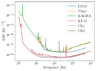
Figure 1: Amplitude spectral density for 2G and 3G detectors.

Detector	Latitude	Longitude	x-arm azimuth	y-arm azimuth	$f_{ini}\,[\text{Hz}]$
ET-1	0.7615	0.1833	0.3392	5.5752	1
ET-2	0.7629	0.1841	4.5280	3.4808	1
ET-3	0.7627	0.1819	2.4336	1.3864	1
CE1	0.7613	$-2.0281$	1.5708	0	5
CE2	$-0.5811$	2.6021	2.3562	0.7854	5

Table 1: Localization and the power spectral density lowest frequency of the detectors considered in this study.

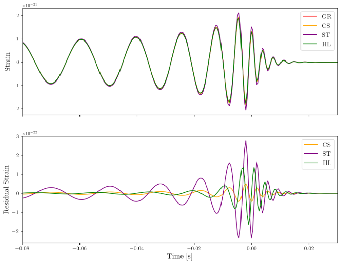
Figure 2: Top panel: waveforms for a GW150914-like event for different values of the $\bm{\theta}_{\text{PPE}}$ parameters. Bottom panel: residual strain, i.e., $\tilde{h}_{\text{GR}}-\tilde{h}_{\text{PPE}}$, for the different theories under consideration in this work.

IV Observational constraints

In this Section, we study the power constraint of 3G detectors on parity-violating theories. In particular, we focus on the capabilities of ET and CE. For ET, we consider a triangular-shaped configuration of 3 independent detectors co-located in Italy (ET-1, ET-2, ET-3) by using the 10 km arm ET-D noise curve model. While, for CE, we consider 2 independent L-shaped detectors: the first placed in the United States (CE1) and the second one in Australia (CE2), with 40 and 20 km arm lengths, respectively. In Fig. 1, we depict the detector’s amplitude spectral density (ASD) for the 2G (LVK) and 3G detectors. Furthermore, in Table 1, we describe the main features of the interferometers: the localization, the orientation and the lowest frequency of the power spectral density. In the present analysis, we consider the following configurations: ET, ET and CE1 (ET + CE1), and ET along with the two CE detectors (ET + CE1 + CE2).

We model the quantity $\tilde{h}_{\text{GR}}$ in Eq. (32) with the IMRPhenomD waveform, considering an orbital configurations with spins aligned with the angular momentum. Within this prescription, the set of binary parameters is $\mathcal{B}=\{\mathcal{M},\,q,\,d_{L},\,\theta_{jn},\,t_{c},\,\phi_{c},\,\psi,\,\chi_{1},\,\chi_{2},\,ra,\,dec,\,\bm{\theta}_{\text{PPE}}\}$. We can distinguish the extrinsic and intrinsic parameters. The former include the sky angles ($ra$, $dec$), the inclination $\theta_{jn}$, the polarization angle $\psi$, the phase at coalescence $\phi_{c}$, the coalescence time $t_{c}$, and the luminosity distance of the source, $d_{L}$. On the other hand, the intrinsic parameters are the chirp mass $\mathcal{M}$, the mass ratio $q$, and the projection $\chi_{i}$ of the $i$-th spin along $z$. Besides the binary parameters, in the present analysis, we consider the PPE expansion parameters, i.e., $\bm{\theta}_{\text{PPE}}$.

To simulate the injection and to analyze the GW waveform, we adopt the open software bilby [82, 83]. The synthetic signal is taken into account by assuming the system parameters as in the event GW150914 [84]. Furthermore, the PPE parameters are set to their corresponding GR fiducial values. The fiducial values for the binary parameters are reported in Table 2. In Fig. 2, we highlight the differences in the waveform when the $\bm{\theta}_{\text{PPE}}$ parameters are not vanishing.

Assuming the detector noise to be stochastic, stationary and a Gaussian function of time, we can evaluate the signal-to-noise ratio (SNR) through the expression

$$\text{SNR}=\sqrt{\langle h,h\rangle}\,,$$ (103)

where the inner product $\langle\cdot,\cdot\rangle$ is defined as

$$\langle A,B\rangle=4\,\text{Re}\int_{0}^{\infty}\frac{\tilde{A}^{*}(f)\tilde{B}(f)}{S_{n}(f)}df\,,$$ (104)

and $S_{n}(f)$ is the one-side power spectrum of the detector. For a network of $N$ detectors, the total SNR is given by

$$\text{SNR}_{N}=\sqrt{\sum_{i=1}^{N}\text{SNR}^{2}_{i}}\,.$$ (105)

The estimated SNR values for the injected signal are 935, 1740 and 1811 for the ET, ET + CE1 and ET + CE1 + CE2 networks, respectively. Since the SNR is very high, we expect the localization parameters ($ra,\,dec,\,\psi,\,\theta_{jn}$) to be weakly correlated with the intrinsic parameters. Hence, we fix these parameters to their fiducial values. In so doing, the inference parameter set reduces to

$$\mathcal{B}=\{\mathcal{M},q,d_{L},\,t_{c},\,\phi_{c},\,\chi_{1},\,\chi_{2},\,\bm{\theta}_{\text{PPE}}\}.$$ (106)

Parameter	Value	Parameter	Value
$\mathcal{M}\,[M_{\odot}]$	28.1	$\psi$ [rad]	2.66
$q$	0.81	$ra$ [rad]	1.38
$d_{L}\,[\text{Mpc}]$	400	$dec$ [rad]	$-1.21$
$\chi_{1}$	0.31	$\theta_{jn}$ [rad]	0.40
$\chi_{2}$	0.39	$\phi_{c}$ [rad]	1.30
$t_{c}\,[\text{s}]$	0.00	$\bm{\theta}_{\text{PPE}}$	0.00

Table 2: Injection parameters for the binary system.

Therefore, we sample the posterior distributions by the bilby-mcmc algorithm [85], using the priors shown in Table 3. In our numerical analysis, we marginalize over the phase $\phi_{c}$ and coalescence time $t_{c}$, and we set the minimum frequency to $10$ Hz and the maximum frequency to $1024$ Hz. Additionally, we fix $H_{0}=67.7$ km s^-1 Mpc^-1 and $\Omega_{m0}=0.308$ in order to convert the $d_{L}$ sampling into that over $z$. In what follows, we shall present separately the numerical constraints on the PPE parameters for the different theoretical scenarios under study.

Parameter	Prior
$\mathcal{M}\,[M_{\odot}]$	$\mathcal{U}(20,100)$
$q$	$\mathcal{U}(0.125,1)$
$d_{L}\,[\text{Mpc}]$	$\mathcal{U}(100,5000)$
$\chi_{1}$	$\mathcal{U}(-1,1)$
$\chi_{2}$	$\mathcal{U}(-1,1)$
$\bm{\theta}_{\text{PPE}}$	$\mathcal{U}(-500,500)$

Table 3: Priors for the free parameters of the sampling, where $\mathcal{U}$ indicates a uniform distribution function.

IV.1 Chern-Simons gravity

Based on Eqs. (49) and (50), the PPE parameter for CS gravity is

$$\bm{\theta}_{\text{PPE}}=\frac{\alpha_{1_{0}}}{M_{\text{PV}}}\,.$$ (107)

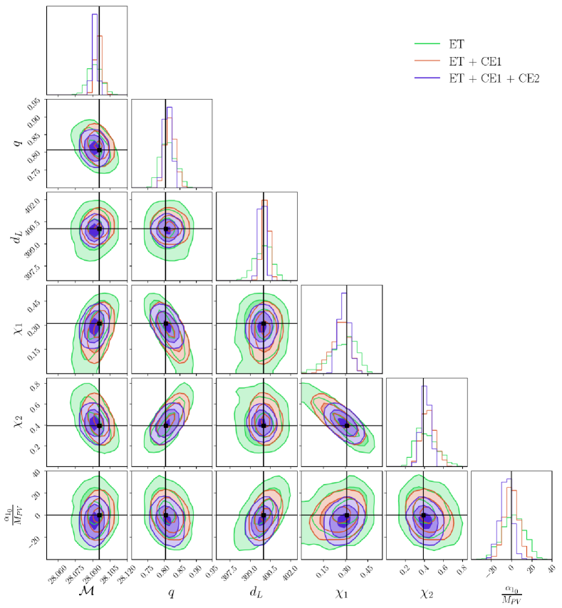
Figure 3: 68%, 95% and 99% C.L. contours, with posterior distributions, for the free parameters of CS gravity under different detector configurations. The straight lines indicate the injected values of the GW parameters.

In Table 4a, we present the results of our analysis for the different detector networks, whereas, in Fig. 3, we show the $1\sigma$, $2\sigma$ and $3\sigma$ confidence level (C.L.) regions and the posterior distributions of the GW parameters. In particular, we note that the PPE parameter is weakly correlated with $d_{L}$ and $\chi_{1}$. The PPE parameter is constrained with an accuracy of $(10.93,\,6.70,\,5.91)\,M_{\odot}$ for ET, ET + CE1 and ET + CE1 + CE2, respectively.

In Fig. 4, we compare the results obtained from 3G detectors with the ones of the 2G detector network. Specifically, we show the deviations of the posterior distributions from the injected values of the GW parameters. In this respect, we highlight an improvement on the PPE parameter of a factor $\sim 18$.

IV.2 Symmetric teleparallel gravity

In view of Eqs. (80) to (83), we can define the PPE parameter set in ST gravity as follows:

$$\bm{\theta}_{\text{PPE}}=\left\{\frac{\alpha_{1_{0}}}{M_{\text{PV}}},\,\beta_{1_{0}},\,\frac{\delta_{2_{0}}}{M_{\text{PV}}}\right\}.$$ (108)

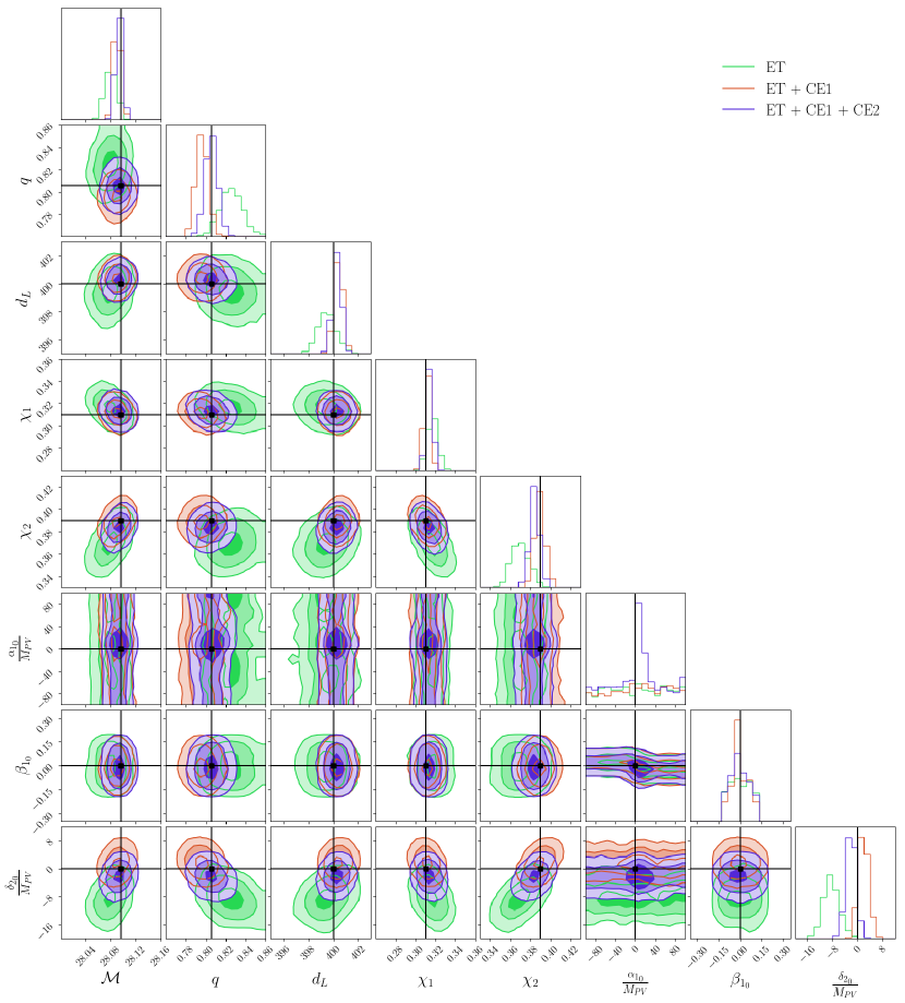
Figure 5: 68%, 95% and 99% C.L. contours, with posterior distributions, for the free parameters of ST gravity under different detector configurations. The straight lines indicate the injected values of the GW parameters.

Our MCMC results are listed in Table 4b and plotted in Fig. 5. It is worth noticing that $\frac{\alpha_{1_{0}}}{M_{\text{PV}}}$ turns out to be unconstrained in all configurations. On the other hand, the parameter $\beta_{1_{0}}$ is bounded with an accuracy of 0.08, 0.06 and 0.074 under the ET, ET + CE1 and ET + CE1 + CE2 configurations, respectively. The same detector networks are capable of constraining $\frac{\delta_{2_{0}}}{M_{\text{PV}}}$ with an accuracy of $(2.52,\,1.70,\,1.53)\,M_{\odot}^{2}\,\text{Mpc}^{-1}$, respectively.

The results obtained for the 3G and 2G detector networks are compared in Fig. 6. We note that $\frac{\alpha_{1_{0}}}{M_{\text{PV}}}$ remains unconstrained also for the 2G detectors. Moreover, the two configurations provide similar accuracy on the parameter $\beta_{1_{0}}$. However, the posterior distribution of the latter from the 3G detectors peaks around $0$, while the result of the 2G detectors is almost flat in the same confidence interval. Finally, the 3G detector network improves the accuracy on $\frac{\delta_{2_{0}}}{M_{\text{PV}}}$ by a factor $\sim 15$.

IV.3 Hořava-Lifshitz gravity

The PPE parameter set in the case of HL gravity is provided by Eqs. (99) to (102):

$$\bm{\theta}_{\text{PPE}}=\left\{\frac{\delta_{2_{0}}}{M_{\text{PV}}},\,\frac{\delta_{4_{0}}}{M_{\text{PV}}^{3}}\right\}.$$ (109)

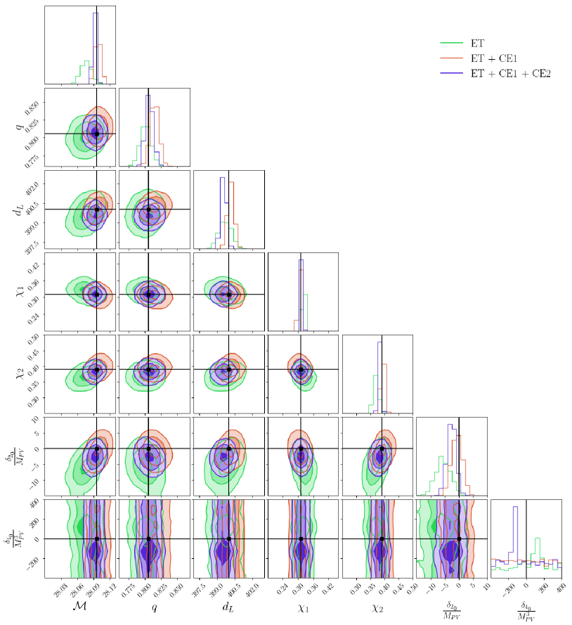
Figure 7: 68%, 95% and 99% C.L. contours, with posterior distributions, for the free parameters of HL gravity under different detector configurations. The straight lines indicate the injected values of the GW parameters.

We show the posterior distributions in Fig. 7, and the best-fit values of the GW parameters in Table 4c. We can notice that $\frac{\delta_{4_{0}}}{M_{\text{PV}}^{3}}$ is unconstrained, while $\frac{\delta_{2_{0}}}{M_{\text{PV}}}$ is bounded with an accuracy of 2.73, 1.90 and 1.50 under the ET, ET + CE1 and ET + CE1 + CE2 networks, respectively.

Furthermore, Fig. 8 highlights the improvement one may obtain by means of 3G detectors compared to the 2G detector network. In fact, the accuracy on $\frac{\delta_{2_{0}}}{M_{\text{PV}}}$ increase by a factor $\sim 19$.

Network	$\mathcal{M}\,[M_{\odot}]$	$q$	$d_{L}\,[\text{Mpc}]$	$\chi_{1}$	$\chi_{2}$	$\frac{\alpha_{1_{0}}}{M_{\text{PV}}}\,[M_{\odot}]$
ET	$28.09^{+0.01}_{-0.01}$	$0.81^{+0.03}_{-0.02}$	$400.02^{+0.58}_{-0.67}$	$0.29^{+0.08}_{-0.11}$	$0.41^{+0.12}_{-0.10}$	$1.82^{+11.04}_{-10.83}$
ET + CE1	$28.092^{+0.003}_{-0.003}$	$0.81^{+0.02}_{-0.02}$	$400.14^{+0.27}_{-0.25}$	$0.27^{+0.05}_{-0.07}$	$0.44^{+0.08}_{-0.07}$	$-0.28^{+6.91}_{-6.49}$
ET + CE1 + CE2	$28.092^{+0.002}_{-0.002}$	$0.81^{+0.01}_{-0.01}$	$399.88^{+0.20}_{-0.22}$	$0.29^{+0.04}_{-0.04}$	$0.41^{+0.05}_{-0.05}$	$-5.27^{+5.47}_{-6.35}$

(a) CS gravity

Network	$\mathcal{M}\,[M_{\odot}]$	$q$	$d_{L}\,[\text{Mpc}]$	$\chi_{1}$	$\chi_{2}$	$\frac{\alpha_{1_{0}}}{M_{\text{PV}}}\,[M_{\odot}]$	$\beta_{1_{0}}\,[\text{Mpc}^{-1}]$	$\frac{\delta_{2_{0}}}{M_{\text{PV}}}\,[M_{\odot}^{2}\,\text{Mpc}^{-1}]$
ET	$28.08^{+0.01}_{-0.01}$	$0.81^{+0.01}_{-0.01}$	$399.47^{+0.79}_{-0.73}$	$0.32^{+0.01}_{-0.01}$	$0.37^{+0.01}_{-0.01}$	n.c.	$0.00^{+0.08}_{-0.08}$	$-1.12^{+2.72}_{-2.33}$
ET + CE1	$28.090^{+0.005}_{-0.005}$	$0.796^{+0.006}_{-0.006}$	$400.39^{+0.36}_{-0.34}$	$0.312^{+0.003}_{-0.003}$	$0.389^{+0.005}_{-0.005}$	n.c.	$-0.03^{+0.09}_{-0.03}$	$1.79^{+1.78}_{-1.63}$
ET + CE1 + CE2	$28.093^{+0.005}_{-0.005}$	$0.805^{+0.006}_{-0.006}$	$400.26^{+0.32}_{-0.33}$	$0.314^{+0.003}_{-0.003}$	$0.384^{+0.005}_{-0.005}$	n.c.	$-0.002^{+0.074}_{-0.074}$	$-2.19^{+1.55}_{-1.52}$

(b) ST gravity

Network	$\mathcal{M}\,[M_{\odot}]$	$q$	$d_{L}\,[\text{Mpc}]$	$\chi_{1}$	$\chi_{2}$	$\frac{\delta_{2_{0}}}{M_{\text{PV}}}\,[M_{\odot}^{2}\,\text{Mpc}^{-1}]$	$\frac{\delta_{4_{0}}}{M_{\text{PV}}^{3}}\,[M_{\odot}^{4}\,\text{Mpc}^{-1}]$
ET	$28.08^{+0.01}_{-0.01}$	$0.80^{+0.01}_{-0.01}$	$399.67^{+0.54}_{-0.51}$	$0.32^{+0.01}_{-0.01}$	$0.37^{+0.01}_{-0.01}$	$-5.76^{+2.94}_{-2.53}$	n.c.
ET + CE1	$28.100^{+0.007}_{-0.007}$	$0.82^{+0.01}_{-0.01}$	$400.17^{+0.25}_{-0.28}$	$0.306^{+0.004}_{-0.004}$	$0.393^{+0.006}_{-0.006}$	$-0.81^{+1.94}_{-1.87}$	n.c.
ET + CE1 + CE2	$28.092^{+0.003}_{-0.003}$	$0.807^{+0.006}_{-0.006}$	$399.56^{+0.21}_{-0.21}$	$0.314^{+0.003}_{-0.003}$	$0.383^{+0.004}_{-0.004}$	$-2.70^{+1.50}_{-1.50}$	n.c.

(c) HL gravity

Table 4: Best-fit values and 1$\sigma$ uncertainties on the GW parameters of the theoretical scenarios under study, for different detector configurations. n.c. stands for not constrained.

V Summary and discussion

We considered parity violation in the propagation of GWs through a newly proposed PPE formalism. In particular, we framed deviations from GR by means of a general parametrized framework taking into account the modified amplitude and phase of GWs. We thus focused on the specific cases of CS, ST and HL gravity, where departures from Einstein’s theory may emerge from additional parity-violating terms included in the gravitational action. In so doing, we first discussed the main features of the theoretical scenarios under study. Then, we outlined the geometrical and physical characteristics of future ground-based GW interferometers, namely ET and CE, and showed how they can be used to probe parity violation.

Hence, we described the methodology to constrain the PPE expansion parameters associated with the aforementioned parity-violating theories. Using the sensitivities of 3G detectors, we simulated GW signals from binary systems, such as BBH and BNS, and we obtained $68\%$, $95\%$ and $99\%$ numerical bounds on both binary and PPE parameters, for different GW detector networks. Furthermore, we compared the results of the combined 3G detectors with those resulting from the 2G detector configuration of LVK interferometers. For each parity-violating model, we showed the deviations of the posterior density distributions for the fitting parameters with respect to the injected GR signal.

It is worth mentioning that the accuracy of the GW and PPE parameters increases when more detectors are considered in the network, independently from the theoretical framework. As the SNR is very high, the uncertainties on the GW parameters turn out to be quite low. Indeed, for all models under study, we constrained the chirp mass and mass ratio with a relative accuracy of $\sim(0.04,\,0.03,\,0.01)\%$ and $\sim(3,\,1.5,\,1)\%$ for ET, ET + CE1 and ET + CE1 + CE2, respectively. Additionally, the precision on the luminosity distance spans from $\sim 0.2\%$ in the case of ET alone, to $\sim 0.1\%$ and $\sim 0.08\%$ when ET is together with one or two CE detectors in the same network. Moreover, we bounded the spin parameter $\chi_{1}$ with a relative accuracy of $\sim(20,\,10,\,3)\%$ and $\sim(20,\,10,\,2)\%$ for the three detector configurations, respectively.

Our results indicate an improvement of roughly one order of magnitude with respect to those obtained for the 2G detectors. Specifically, from the LVK configuration, we obtained a relative accuracy of $0.5\%$ on the chirp mass, $7\%$ on the mass ratio, $1.6\%$ on the luminosity distance, and $63\%$ and $80\%$ on $\chi_{1}$ and $\chi_{2}$, respectively. It is worth noticing that the constraint on the $\tilde{h}_{\text{GR}}$ waveform parameters are almost independent of the theoretical model also under the LVK analysis.

As regards the PPE parameters, we found that one of them remains unconstrained in ST and HL gravity. This feature may be related to the low-frequency cut-off. In fact, in order to reduce the computational time, we fixed the minimum frequency of $10$ Hz. However, one might extend the analysis to the 1-10 Hz frequency band, and increase the duration of the signal. This would further improve the constraints on the GW parameters.

Finally, it is important to stress that the PPE parameters enter the waveform at higher orders of the PN expansion. Hence, a more accurate waveform would be needed in the future, in order to detect with more accuracy deviations from GR emerging from parity-violating theories.

Figure 4: Deviations of the posterior probability distributions from the injected values of the GW parameters for CS gravity. The injected signal is analyzed both for the 3G detector (ET + CE1+ CE2) and 2G detector (LVK) configurations. The horizontal dashed lines indicate zero deviations from the injected signal.

Figure 6: Deviations of the posterior probability distributions from the injected values of the GW parameters for ST gravity. The injected signal is analyzed both for the 3G detector (ET + CE1+ CE2) and 2G detector (LVK) configurations. The horizontal dashed lines indicate zero deviations from the injected signal.

Figure 8: Deviations of the posterior probability distributions from the injected values of the GW parameters for HL gravity. The injected signal is analyzed both for the 3G detector (ET + CE1+ CE2) and 2G detector (LVK) configurations. The horizontal dashed lines indicate zero deviations from the injected signal.

References

- Abbott et al. [2017] B. P. Abbott et al. (LIGO Scientific, Virgo, Fermi-GBM, INTEGRAL), Gravitational Waves and Gamma-rays from a Binary Neutron Star Merger: GW170817 and GRB 170817A, Astrophys. J. Lett. 848, L13 (2017), arXiv:1710.05834 [astro-ph.HE] .
- Abbott et al. [2019a] B. P. Abbott et al. (LIGO Scientific, Virgo), GWTC-1: A Gravitational-Wave Transient Catalog of Compact Binary Mergers Observed by LIGO and Virgo during the First and Second Observing Runs, Phys. Rev. X 9, 031040 (2019a), arXiv:1811.12907 [astro-ph.HE] .
- Abbott et al. [2021] R. Abbott et al. (LIGO Scientific, VIRGO, KAGRA), GWTC-3: Compact Binary Coalescences Observed by LIGO and Virgo During the Second Part of the Third Observing Run, (2021), arXiv:2111.03606 [gr-qc] .
- Ezquiaga and Zumalacárregui [2017] J. M. Ezquiaga and M. Zumalacárregui, Dark Energy After GW170817: Dead Ends and the Road Ahead, Phys. Rev. Lett. 119, 251304 (2017), arXiv:1710.05901 [astro-ph.CO] .
- Farrugia et al. [2018] G. Farrugia, J. Levi Said, V. Gakis, and E. N. Saridakis, Gravitational Waves in Modified Teleparallel Theories, Phys. Rev. D 97, 124064 (2018), arXiv:1804.07365 [gr-qc] .
- Belgacem et al. [2018a] E. Belgacem, Y. Dirian, S. Foffa, and M. Maggiore, Modified gravitational-wave propagation and standard sirens, Phys. Rev. D 98, 023510 (2018a), arXiv:1805.08731 [gr-qc] .
- Järv et al. [2018] L. Järv, M. Rünkla, M. Saal, and O. Vilson, Nonmetricity formulation of general relativity and its scalar-tensor extension, Phys. Rev. D 97, 124025 (2018), arXiv:1802.00492 [gr-qc] .
- Abbott et al. [2019b] B. P. Abbott et al. (LIGO Scientific, Virgo), Tests of General Relativity with GW170817, Phys. Rev. Lett. 123, 011102 (2019b), arXiv:1811.00364 [gr-qc] .
- Abbott et al. [2019c] B. P. Abbott et al. (LIGO Scientific, Virgo), Tests of General Relativity with the Binary Black Hole Signals from the LIGO-Virgo Catalog GWTC-1, Phys. Rev. D 100, 104036 (2019c), arXiv:1903.04467 [gr-qc] .
- Bengochea and Ferraro [2009] G. R. Bengochea and R. Ferraro, Dark torsion as the cosmic speed-up, Phys. Rev. D 79, 124019 (2009), arXiv:0812.1205 [astro-ph] .
- Clifton et al. [2012] T. Clifton, P. G. Ferreira, A. Padilla, and C. Skordis, Modified Gravity and Cosmology, Phys. Rept. 513, 1 (2012), arXiv:1106.2476 [astro-ph.CO] .
- D’Agostino and Luongo [2018] R. D’Agostino and O. Luongo, Growth of matter perturbations in nonminimal teleparallel dark energy, Phys. Rev. D 98, 124013 (2018), arXiv:1807.10167 [gr-qc] .
- Nojiri et al. [2017] S. Nojiri, S. D. Odintsov, and V. K. Oikonomou, Modified Gravity Theories on a Nutshell: Inflation, Bounce and Late-time Evolution, Phys. Rept. 692, 1 (2017), arXiv:1705.11098 [gr-qc] .
- D’Agostino [2019] R. D’Agostino, Holographic dark energy from nonadditive entropy: cosmological perturbations and observational constraints, Phys. Rev. D 99, 103524 (2019), arXiv:1903.03836 [gr-qc] .
- Capozziello et al. [2019] S. Capozziello, R. D’Agostino, and O. Luongo, Extended Gravity Cosmography, Int. J. Mod. Phys. D 28, 1930016 (2019), arXiv:1904.01427 [gr-qc] .
- D’Agostino and Nunes [2020] R. D’Agostino and R. C. Nunes, Measurements of in modified gravity theories: The role of lensed quasars in the late-time Universe, Phys. Rev. D 101, 103505 (2020), arXiv:2002.06381 [astro-ph.CO] .
- D’Agostino et al. [2022] R. D’Agostino, O. Luongo, and M. Muccino, Healing the cosmological constant problem during inflation through a unified quasi-quintessence matter field, Class. Quant. Grav. 39, 195014 (2022), arXiv:2204.02190 [gr-qc] .
- Stelle [1978] K. S. Stelle, Classical Gravity with Higher Derivatives, Gen. Rel. Grav. 9, 353 (1978).
- Starobinsky [1980] A. A. Starobinsky, A New Type of Isotropic Cosmological Models Without Singularity, Phys. Lett. B 91, 99 (1980).
- Ferraro and Fiorini [2007] R. Ferraro and F. Fiorini, Modified teleparallel gravity: Inflation without inflaton, Phys. Rev. D 75, 084031 (2007), arXiv:gr-qc/0610067 .
- Deser and Woodard [2007] S. Deser and R. P. Woodard, Nonlocal Cosmology, Phys. Rev. Lett. 99, 111301 (2007), arXiv:0706.2151 [astro-ph] .
- Sotiriou and Faraoni [2010] T. P. Sotiriou and V. Faraoni, f(R) Theories Of Gravity, Rev. Mod. Phys. 82, 451 (2010), arXiv:0805.1726 [gr-qc] .
- Capozziello et al. [2022] S. Capozziello, R. D’Agostino, and O. Luongo, The phase-space view of non-local gravity cosmology, Phys. Lett. B 834, 137475 (2022), arXiv:2207.01276 [gr-qc] .
- Bajardi and D’Agostino [2023] F. Bajardi and R. D’Agostino, Late-time constraints on modified Gauss-Bonnet cosmology, Gen. Rel. Grav. 55, 49 (2023), arXiv:2208.02677 [gr-qc] .
- Capozziello and D’Agostino [2023] S. Capozziello and R. D’Agostino, Reconstructing the distortion function of non-local cosmology: A model-independent approach, Phys. Dark Univ. 42, 101346 (2023), arXiv:2310.03136 [gr-qc] .
- Mirshekari et al. [2012] S. Mirshekari, N. Yunes, and C. M. Will, Constraining Generic Lorentz Violation and the Speed of the Graviton with Gravitational Waves, Phys. Rev. D 85, 024041 (2012), arXiv:1110.2720 [gr-qc] .
- Mewes [2019] M. Mewes, Signals for Lorentz violation in gravitational waves, Phys. Rev. D 99, 104062 (2019), arXiv:1905.00409 [gr-qc] .
- Ezquiaga et al. [2021] J. M. Ezquiaga, W. Hu, M. Lagos, and M.-X. Lin, Gravitational wave propagation beyond general relativity: waveform distortions and echoes, JCAP 11 (11), 048, arXiv:2108.10872 [astro-ph.CO] .
- Gong et al. [2023] C. Gong, T. Zhu, R. Niu, Q. Wu, J.-L. Cui, X. Zhang, W. Zhao, and A. Wang, Gravitational wave constraints on nonbirefringent dispersions of gravitational waves due to Lorentz violations with GWTC-3 events, Phys. Rev. D 107, 124015 (2023), arXiv:2302.05077 [gr-qc] .
- Kostelecký and Mewes [2016] V. A. Kostelecký and M. Mewes, Testing local Lorentz invariance with gravitational waves, Phys. Lett. B 757, 510 (2016), arXiv:1602.04782 [gr-qc] .
- Nishizawa and Kobayashi [2018] A. Nishizawa and T. Kobayashi, Parity-violating gravity and GW170817, Phys. Rev. D 98, 124018 (2018), arXiv:1809.00815 [gr-qc] .
- Nair et al. [2019] R. Nair, S. Perkins, H. O. Silva, and N. Yunes, Fundamental Physics Implications for Higher-Curvature Theories from Binary Black Hole Signals in the LIGO-Virgo Catalog GWTC-1, Phys. Rev. Lett. 123, 191101 (2019), arXiv:1905.00870 [gr-qc] .
- Wang et al. [2022] Y.-F. Wang, S. M. Brown, L. Shao, and W. Zhao, Tests of gravitational-wave birefringence with the open gravitational-wave catalog, Phys. Rev. D 106, 084005 (2022), arXiv:2109.09718 [astro-ph.HE] .
- Jenks et al. [2023] L. Jenks, L. Choi, M. Lagos, and N. Yunes, Parametrized parity violation in gravitational wave propagation, Phys. Rev. D 108, 044023 (2023), arXiv:2305.10478 [gr-qc] .
- Lue et al. [1999] A. Lue, L.-M. Wang, and M. Kamionkowski, Cosmological signature of new parity violating interactions, Phys. Rev. Lett. 83, 1506 (1999), arXiv:astro-ph/9812088 .
- Alexander and Yunes [2009] S. Alexander and N. Yunes, Chern-Simons Modified General Relativity, Phys. Rept. 480, 1 (2009), arXiv:0907.2562 [hep-th] .
- Kawai and Kim [2019] S. Kawai and J. Kim, Gauss–Bonnet Chern–Simons gravitational wave leptogenesis, Phys. Lett. B 789, 145 (2019), arXiv:1702.07689 [hep-th] .
- Bajardi et al. [2021] F. Bajardi, D. Vernieri, and S. Capozziello, Exact solutions in higher-dimensional Lovelock and AdS5 Chern-Simons gravity, JCAP 11 (11), 057, arXiv:2106.07396 [gr-qc] .
- Sulantay et al. [2023] F. Sulantay, M. Lagos, and M. Bañados, Chiral gravitational waves in Palatini-Chern-Simons gravity, Phys. Rev. D 107, 104025 (2023), arXiv:2211.08925 [gr-qc] .
- Green et al. [1988] M. B. Green, J. H. Schwarz, and E. Witten, Superstring Theory. Vol. 2: Loop Amplitudes, Anomalies and Phenomenology (1988).
- Crisostomi et al. [2018] M. Crisostomi, K. Noui, C. Charmousis, and D. Langlois, Beyond Lovelock gravity: Higher derivative metric theories, Phys. Rev. D 97, 044034 (2018), arXiv:1710.04531 [hep-th] .
- Zhao et al. [2020a] W. Zhao, T. Zhu, J. Qiao, and A. Wang, Waveform of gravitational waves in the general parity-violating gravities, Phys. Rev. D 101, 024002 (2020a), arXiv:1909.10887 [gr-qc] .
- Beltrán Jiménez et al. [2018] J. Beltrán Jiménez, L. Heisenberg, and T. Koivisto, Coincident General Relativity, Phys. Rev. D 98, 044048 (2018), arXiv:1710.03116 [gr-qc] .
- Conroy and Koivisto [2019] A. Conroy and T. Koivisto, Parity-Violating Gravity and GW170817 in Non-Riemannian Cosmology, JCAP 12, 016, arXiv:1908.04313 [gr-qc] .
- Capozziello and D’Agostino [2022] S. Capozziello and R. D’Agostino, Model-independent reconstruction of f(Q) non-metric gravity, Phys. Lett. B 832, 137229 (2022), arXiv:2204.01015 [gr-qc] .
- Horava [2009] P. Horava, Quantum Gravity at a Lifshitz Point, Phys. Rev. D 79, 084008 (2009), arXiv:0901.3775 [hep-th] .
- Zhu et al. [2013] T. Zhu, W. Zhao, Y. Huang, A. Wang, and Q. Wu, Effects of parity violation on non-gaussianity of primordial gravitational waves in Hořava-Lifshitz gravity, Phys. Rev. D 88, 063508 (2013), arXiv:1305.0600 [hep-th] .
- Yunes and Pretorius [2009] N. Yunes and F. Pretorius, Fundamental Theoretical Bias in Gravitational Wave Astrophysics and the Parameterized Post-Einsteinian Framework, Phys. Rev. D 80, 122003 (2009), arXiv:0909.3328 [gr-qc] .
- Cornish et al. [2011] N. Cornish, L. Sampson, N. Yunes, and F. Pretorius, Gravitational Wave Tests of General Relativity with the Parameterized Post-Einsteinian Framework, Phys. Rev. D 84, 062003 (2011), arXiv:1105.2088 [gr-qc] .
- Huwyler et al. [2012] C. Huwyler, A. Klein, and P. Jetzer, Testing General Relativity with LISA including Spin Precession and Higher Harmonics in the Waveform, Phys. Rev. D 86, 084028 (2012), arXiv:1108.1826 [gr-qc] .
- Loutrel et al. [2023] N. Loutrel, P. Pani, and N. Yunes, Parametrized post-Einsteinian framework for precessing binaries, Phys. Rev. D 107, 044046 (2023), arXiv:2210.10571 [gr-qc] .
- Zhao et al. [2020b] W. Zhao, T. Liu, L. Wen, T. Zhu, A. Wang, Q. Hu, and C. Zhou, Model-independent test of the parity symmetry of gravity with gravitational waves, Eur. Phys. J. C 80, 630 (2020b), arXiv:1909.13007 [gr-qc] .
- Wang et al. [2021] Y.-F. Wang, R. Niu, T. Zhu, and W. Zhao, Gravitational Wave Implications for the Parity Symmetry of Gravity in the High Energy Region, Astrophys. J. 908, 58 (2021), arXiv:2002.05668 [gr-qc] .
- Okounkova et al. [2022] M. Okounkova, W. M. Farr, M. Isi, and L. C. Stein, Constraining gravitational wave amplitude birefringence and Chern-Simons gravity with GWTC-2, Phys. Rev. D 106, 044067 (2022), arXiv:2101.11153 [gr-qc] .
- Maggiore et al. [2020] M. Maggiore et al., Science Case for the Einstein Telescope, JCAP 03, 050, arXiv:1912.02622 [astro-ph.CO] .
- Branchesi et al. [2023] M. Branchesi et al., Science with the Einstein Telescope: a comparison of different designs, JCAP 07, 068, arXiv:2303.15923 [gr-qc] .
- Reitze et al. [2019] D. Reitze et al., Cosmic Explorer: The U.S. Contribution to Gravitational-Wave Astronomy beyond LIGO, Bull. Am. Astron. Soc. 51, 035 (2019), arXiv:1907.04833 [astro-ph.IM] .
- Evans et al. [2021] M. Evans et al., A Horizon Study for Cosmic Explorer: Science, Observatories, and Community, (2021), arXiv:2109.09882 [astro-ph.IM] .
- Cai and Yang [2017] R.-G. Cai and T. Yang, Estimating cosmological parameters by the simulated data of gravitational waves from the Einstein Telescope, Phys. Rev. D 95, 044024 (2017), arXiv:1608.08008 [astro-ph.CO] .
- Belgacem et al. [2018b] E. Belgacem, Y. Dirian, S. Foffa, and M. Maggiore, Gravitational-wave luminosity distance in modified gravity theories, Phys. Rev. D 97, 104066 (2018b), arXiv:1712.08108 [astro-ph.CO] .
- Nishizawa and Arai [2019] A. Nishizawa and S. Arai, Generalized framework for testing gravity with gravitational-wave propagation. III. Future prospect, Phys. Rev. D 99, 104038 (2019), arXiv:1901.08249 [gr-qc] .
- D’Agostino and Nunes [2019] R. D’Agostino and R. C. Nunes, Probing observational bounds on scalar-tensor theories from standard sirens, Phys. Rev. D 100, 044041 (2019), arXiv:1907.05516 [gr-qc] .
- Bonilla et al. [2020] A. Bonilla, R. D’Agostino, R. C. Nunes, and J. C. N. de Araujo, Forecasts on the speed of gravitational waves at high , JCAP 03, 015, arXiv:1910.05631 [gr-qc] .
- Kalomenopoulos et al. [2021] M. Kalomenopoulos, S. Khochfar, J. Gair, and S. Arai, Mapping the inhomogeneous Universe with standard sirens: degeneracy between inhomogeneity and modified gravity theories, Mon. Not. Roy. Astron. Soc. 503, 3179 (2021), arXiv:2007.15020 [astro-ph.CO] .
- Mukherjee et al. [2021] S. Mukherjee, B. D. Wandelt, and J. Silk, Testing the general theory of relativity using gravitational wave propagation from dark standard sirens, Mon. Not. Roy. Astron. Soc. 502, 1136 (2021), arXiv:2012.15316 [astro-ph.CO] .
- Baker and Harrison [2021] T. Baker and I. Harrison, Constraining Scalar-Tensor Modified Gravity with Gravitational Waves and Large Scale Structure Surveys, JCAP 01, 068, arXiv:2007.13791 [astro-ph.CO] .
- Tasinato et al. [2021] G. Tasinato, A. Garoffolo, D. Bertacca, and S. Matarrese, Gravitational-wave cosmological distances in scalar-tensor theories of gravity, JCAP 06, 050, arXiv:2103.00155 [gr-qc] .
- Allahyari et al. [2022] A. Allahyari, R. C. Nunes, and D. F. Mota, No slip gravity in light of LISA standard sirens, Mon. Not. Roy. Astron. Soc. 514, 1274 (2022), arXiv:2110.07634 [astro-ph.CO] .
- Califano et al. [2023a] M. Califano, I. de Martino, D. Vernieri, and S. Capozziello, Constraining CDM cosmological parameters with Einstein Telescope mock data, Mon. Not. Roy. Astron. Soc. 518, 3372 (2023a), arXiv:2205.11221 [astro-ph.CO] .
- D’Agostino and Nunes [2022] R. D’Agostino and R. C. Nunes, Forecasting constraints on deviations from general relativity in f(Q) gravity with standard sirens, Phys. Rev. D 106, 124053 (2022), arXiv:2210.11935 [gr-qc] .
- Califano et al. [2023b] M. Califano, I. de Martino, D. Vernieri, and S. Capozziello, Exploiting the Einstein Telescope to solve the Hubble tension, Phys. Rev. D 107, 123519 (2023b), arXiv:2208.13999 [astro-ph.CO] .
- D’Agostino et al. [2023] R. D’Agostino, M. Califano, N. Menadeo, and D. Vernieri, Role of spatial curvature in the primordial gravitational wave power spectrum, Phys. Rev. D 108, 043538 (2023), arXiv:2305.14238 [astro-ph.CO] .
- Yunes et al. [2010] N. Yunes, R. O’Shaughnessy, B. J. Owen, and S. Alexander, Testing gravitational parity violation with coincident gravitational waves and short gamma-ray bursts, Phys. Rev. D 82, 064017 (2010), arXiv:1005.3310 [gr-qc] .
- Sathyaprakash and Schutz [2009] B. S. Sathyaprakash and B. F. Schutz, Physics, Astrophysics and Cosmology with Gravitational Waves, Living Rev. Rel. 12, 2 (2009), arXiv:0903.0338 [gr-qc] .
- Damour et al. [2004] T. Damour, A. Gopakumar, and B. R. Iyer, Phasing of gravitational waves from inspiralling eccentric binaries, Phys. Rev. D 70, 064028 (2004), arXiv:gr-qc/0404128 .
- Jackiw and Pi [2003] R. Jackiw and S. Y. Pi, Chern-Simons modification of general relativity, Phys. Rev. D 68, 104012 (2003), arXiv:gr-qc/0308071 .
- Alexander and Martin [2005] S. Alexander and J. Martin, Birefringent gravitational waves and the consistency check of inflation, Phys. Rev. D 71, 063526 (2005), arXiv:hep-th/0410230 .
- Nester and Yo [1999] J. M. Nester and H.-J. Yo, Symmetric teleparallel general relativity, Chin. J. Phys. 37, 113 (1999), arXiv:gr-qc/9809049 .
- Zhu et al. [2011] T. Zhu, Q. Wu, A. Wang, and F.-W. Shu, U(1) symmetry and elimination of spin-0 gravitons in Horava-Lifshitz gravity without the projectability condition, Phys. Rev. D 84, 101502 (2011), arXiv:1108.1237 [hep-th] .
- Zhu et al. [2012] T. Zhu, F.-W. Shu, Q. Wu, and A. Wang, General covariant Horava-Lifshitz gravity without projectability condition and its applications to cosmology, Phys. Rev. D 85, 044053 (2012), arXiv:1110.5106 [hep-th] .
- Muttoni et al. [2023] N. Muttoni, D. Laghi, N. Tamanini, S. Marsat, and D. Izquierdo-Villalba, Dark siren cosmology with binary black holes in the era of third-generation gravitational wave detectors, Phys. Rev. D 108, 043543 (2023), arXiv:2303.10693 [astro-ph.CO] .
- Ashton et al. [2019] G. Ashton et al., BILBY: A user-friendly Bayesian inference library for gravitational-wave astronomy, Astrophys. J. Suppl. 241, 27 (2019), arXiv:1811.02042 [astro-ph.IM] .
- Romero-Shaw et al. [2020] I. M. Romero-Shaw et al., Bayesian inference for compact binary coalescences with bilby: validation and application to the first LIGO–Virgo gravitational-wave transient catalogue, Mon. Not. Roy. Astron. Soc. 499, 3295 (2020), arXiv:2006.00714 [astro-ph.IM] .
- Abbott et al. [2016] B. P. Abbott et al. (LIGO Scientific, Virgo), Observation of Gravitational Waves from a Binary Black Hole Merger, Phys. Rev. Lett. 116, 061102 (2016), arXiv:1602.03837 [gr-qc] .
- Ashton and Talbot [2021] G. Ashton and C. Talbot, B ilby-MCMC: an MCMC sampler for gravitational-wave inference, Mon. Not. Roy. Astron. Soc. 507, 2037 (2021), arXiv:2106.08730 [gr-qc] .