A multiverse model in dS wedge holography

Abstract

We construct a multiverse model based on a recent proposal for dS wedge holography, where empty AdS₃ space is cut off by a pair of accelerated dS₂ space universes, one near the AdS boundary, denoted the UV brane, and one in the AdS interior, the IR brane. We glue together several copies of this configuration along the UV and IR branes in a periodic matter. To provide the model with dynamics of the like near Nariai black holes used in other multiverse toy models, we add dS JT gravity as an intrinsic gravity theory on the IR branes. We then study the entanglement entropy with respect to a UV brane observer, who finds a Page curve transition due to an entanglement island connecting the UV and IR branes. This process involves the coarse-graining of information outside the causally accessible region to the observer. Our model provides an explicit realization of entanglement between IR and UV degrees of freedom encoded in the multiverse.

1 Introduction

Recently, there has been a lot of attention on double holographic models with the development of wedge holography Akal:2020wfl ; Miao:2020oey ; Miao:2021ual , where gravity on an AdS_d+1 region bounded by a pair of end-of-the-world (ETW) branes is dual to a CFT_d-1 theory living on the interception between the branes. This is realized within the Karch-Randall (KR) braneworld models Randall:1999ee ; Randall:1999vf ; Karch:2000gx ; Karch:2000ct ; Giddings:2000mu .

Perhaps one of the most exciting prospects in this program is to learn lessons that can be applied to spacetimes relevant to cosmology. The KR-type of models have received much recent attention for realizing cosmological models Cooper:2018cmb ; Fan:2021eee ; Antonini:2019qkt ; VanRaamsdonk:2021qgv ; Waddell:2022fbn ; Antonini:2022blk ; Antonini:2022xzo ; Antonini:2022opp ; Antonini:2022fna , among several other applications like the information paradox Hawking:2000da ; Cotler:2022weg , or constructing new geometries Emparan:2022ijy , learning about new entries in the holographic dictionary, such as complexity Emparan:2020znc as well as pseudo-entropy Chu:2023zah , among others.

Since the ETW branes in wedge holography can have arbitrary cosmological constants, this has led to different realizations of wedge holography, and importantly for us, to the development of de Sitter (dS) wedge holography Aguilar-Gutierrez:2023tic . Here, one employs a dS_d space ETW branes near the asymptotic boundary of AdS_d+1 space and in the interior bulk geometry, denoted as the ultraviolet (UV) and infrared (IR) branes respectively. Using this setting, one can study different notions of quantum information with respect to an observer living in the UV brane universe, since gravity is not dynamical in this region. In particular, for AdS₃ ambient space, one can analytically reproduce a Page curve with respect to a UV brane observer. Given that pure Einstein gravity is topological in 3-dimensions, one normally either introduces fluctuations in the braneworld location Geng:2022slq ; Geng:2022tfc , or intrinsic gravity theories on the brane. The latter approach has received recent attention in different areas, such as for providing new hints in the context of the information paradox Chen:2020uac ; Chen:2020hmv ; Miao:2023unv ; Li:2023fly , and developing bounds the intrinsic gravity couplings on the ETW branes based on consistency with entanglement velocity Lee:2022efh . The higher curvature corrections to the intrinsic gravity on the brane render the gravity dynamical, as opposed to purely topological. This allows for a more consistent holographic treatment of branes with intrinsic gravity and sharp formulations of quantum information observables Lee:2022efh . Introducing the intrinsic gravitational theory can be used to reproduce a Page curve in a theory with massless gravitons for AdS Karch-Randal braneworlds Miao:2021ual .

Our work aims at exploring the coarse-graining of information encountered in semi-classical quantum cosmology Hartle:2016tpo ; Aguilar-Gutierrez:2021bns within dS wedge holography. In the context of eternal inflation in quantum cosmology, such as quasi-dS₄ space undergoing false vacuum decay into separate universes, one expects that observers in a given universe have access to the information available in other universes given a large amount of redundancy in the theory Aguilar-Gutierrez:2021bns , and yet they cannot interact with those (spacelike separated) universes. This coarse-grained information shares similarities with the fine-grained von Neumann entropy computed with entanglement islands Penington:2019npb ; Almheiri:2019psf , as both are determined from the saddle points from the semi-classical gravitational path integral i.e. a coarse-graining over the allowed geometrical configurations of the theory.

By studying this situation within a braneworld toy model, we gain access to holographic tools to evaluate the holographic entanglement entropy through the HRT formula Ryu:2006bv ; Ryu:2006ef ; Hubeny:2007xt . We can then interpret the information a UV brane observer has access to in terms of CFT degrees of freedom. To carry out this task, we introduce the braneworld model illustrated in Fig 1.

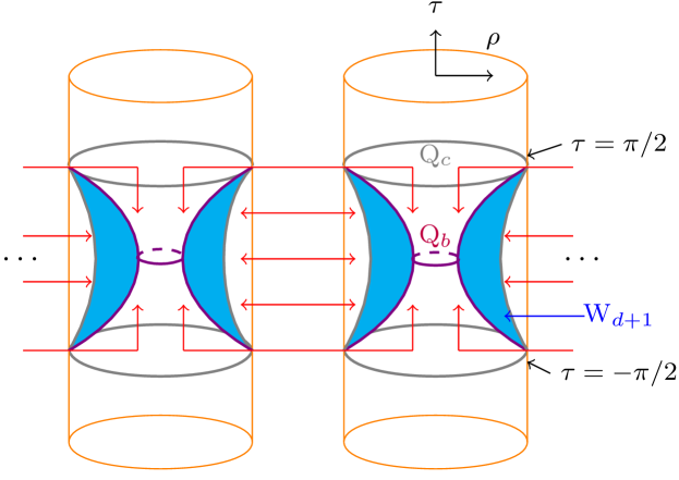
Figure 1: A proposal for a “dS wedge holographic” multiverse formed with a pair of dS_d branes, labeled by Q_b (in purple) and Q_c (gray) embedded in AdS_d+1 space (orange), ending on a pair of codimension-2 Euclidean defects at global AdS time $\tau=\pm\tfrac{\pi}{2}$. The region between the branes (blue) is denoted as the wedge W_d+1. We glue together different copies of the same system along the UV and IR branes (represented by the red arrows) to form a double-sided brane wedge configuration for both the UV and IR branes. From the branes’ perspective, there is a junction between dS_d universes on opposite sides. The respective Penrose diagram is shown in Fig. 2.

This model can be viewed as an extension of dS wedge holography Aguilar-Gutierrez:2023tic . A technical difference with Aguilar-Gutierrez:2023tic is that besides connecting different bulk spacetimes through the dS branes, we also add an intrinsic gravity theory in the IR ETW branes. This allows for the effective braneworld description to contain dynamics even in low spacetime dimensions, in particular for ($2+1$)-dimensional bulk space with dS₂ space branes. We adopt dS Jackiw-Teitelboim (JT) gravity JACKIW1985343 ; TEITELBOIM198341 as the intrinsic theory on the IR branes, while keeping the UV branes to be pure tensional. This is achieved by imposing Dirichlet (Neumann) boundary conditions on the UV (IR) brane, and it allows us to fix the cosmological constant in both the UV and IR branes to be dS space. Having intrinsic gravity on the brane modifies the gravitational observables anchored to the UV boundary, such that we can study the consequences for the properties in the multiverse model.

Our main point of interest is the evolution of holographic entanglement entropy with respect to the CFT degrees of freedom in the UV branes within this model. This construction has an apparent black hole-like information loss paradox. Based on Aguilar-Gutierrez:2023tic , we consider a UV brane observer collecting Hawking radiation. The von Neumann entropy with respect to the UV observer describes two phases; at early times, it is a monotonically increasing function of time during the so-called Hawking phase. The UV observer could access more Hawking modes than the total number of degrees of freedom on the IR brane union with the entangling region in question. However, later there is a phase where it decreases and then saturates, which is an example of the entanglement islands Penington:2019npb ; Almheiri:2019psf .

Our results suggest that the information available to each observer living in a given UV brane completely encodes that of the other universes, given the matching conditions of the configuration. Meanwhile, the ETW branes explicitly realize the coarse-graining of information for observables in quantum cosmology Hartle:2016tpo ; Aguilar-Gutierrez:2021bns . Moreover, the different observers cannot transmit nor decode messages between universes. This observation is consistent with the central dogma Shaghoulian:2021cef and the no-cloning theorem for cosmological horizons discussed in Levine:2022wos . The central dogma in this context refers to encoding information of the spacetime beyond the cosmological horizon, with respect to a given observer, from the interior region. In Levine:2022wos , it was noticed that observers in spacelike separated regions could in principle encode regions of spacetime with some overlap, such that they could reconstruct information from those regions without affecting the ability of the other observer to do the same. This would then enter into tension with the no-cloning theorem. It was noticed that with respect to an observer on a non-dynamical gravity region, this apparent paradox simply does not arise. In that case, the explicit model is an extended near Nariai black hole spacetime. This model has many similarities to ours. The non-dynamical region in our setting refers instead to the UV brane where one collects Hawking radiation. The island transitions show that the RT surfaces will be confined to a single dS wedge universe.

The main new observation, explicit in our model, is the entanglement between the UV and IR degrees of freedom in the coarse-graining of information for the multiverse model.

The rest of this paper is organized as follows. We start by reviewing dS wedge holography and our multiverse model in section 2. In section 3, we present an information recovery protocol and compute the holographic entanglement entropy using the HRT formula before and after the Page transition. We compute and plot the Page curve. In section 3.5 we comment on the connection between our model with the central dogma and non-cloning theorem in the context of quantum cosmology. We conclude in section 4 with a discussion of our findings and important questions to be addressed in the future.

2 Braneworld (multiverse) model

To formulate the multiverse model, we start constructing its building block as a single AdS_d+1 bulk geometry with two ETW branes, one inside the bulk, denoted the IR brane, and the other near the asymptotic boundary, the UV brane. This simple model first appeared in Aguilar-Gutierrez:2023tic as a new proposal for dS wedge holography. In this section, we first review the basic construction involving the single UV and IR brane configuration without intrinsic gravity, later, we introduce multiple brands and the JT couplings on them.

2.1 Review of dS wedge holography

The original proposal in dS wedge holography Aguilar-Gutierrez:2023tic considered a double holographic AdS_d+1 space bounded by a single pair of dS_d space near the asymptotic boundary (denoted as the UV region, where gravity decouples) and an arbitrary location in the bulk interior (the IR region). This brane configuration in the Hartle-Hawking preparation of state corresponds to a tunneling instanton describing membrane creation Aguilar-Gutierrez:2023tic .

There are 3 equivalent ways to describe the system:

• A pair of codimension-2 Euclidean conformal defects on S${}^{1}\times$S^d-2-spaces being timelike separated from each other.

• A pair of entangled dS_d universes with CFT_d matter connected during the infinite past and future via transparent boundary conditions.

• AdS_d+1 bulk space with a pair of dS_d Randall-Sundrum branes Randall:1999ee that overlap at global AdS time $\tau=\pm\tfrac{\pi}{2}$.

The system is described by the following action

$$I= \int_{\hat{\mathcal{M}}}\mathrm{d}^{d+1}x\sqrt{-\hat{g}}\quantity[\tfrac{1}{16\pi G_{d+1}}\quantity(\hat{R}-2\Lambda_{d+1})+\hat{\mathcal{L}}_{\rm bulk}]+\tfrac{1}{8\pi G_{d+1}}\int_{\partial\hat{\mathcal{M}}}\mathrm{d}^{d}x\sqrt{-h}\,K+\sum_{i}I^{(i)}_{\rm matter}\,,$$ (1)

where

$$\Lambda_{d+1}=-\frac{d(d-1)}{2\ell_{d+1}^{2}}\,.$$ (2)

In the above $Q_{i}$ denotes (the worldvolume) of an ETW brane; $h_{\mu\nu}$ is the induced metric on $\partial\mathcal{M}$; $\hat{\mathcal{L}}_{\rm bulk}$ is the bulk field Lagrangian density; $I^{(i)}_{\rm matter}$ is the matter field theory on the $Q_{i}$ brane; and $G_{d+1}$ is Newton’s gravitational constant.

We describe this (empty) spacetime with AdS global coordinates

$$\mathrm{d}s^{2}=\mathrm{d}\rho^{2}-\cosh^{2}\rho\,\mathrm{d}\tau^{2}+\sinh^{2}\rho(\mathrm{d}\alpha^{2}+\cos^{2}\alpha\,\mathrm{d}\Omega_{d-2}^{2})\leavevmode\nobreak\ .$$ (3)

In this foliation, dS branes of arbitrary tension appear can only be found in the range $-\tfrac{\pi}{2}\leq\tau\leq\tfrac{\pi}{2}$ Parikh:2012kg .

We can also employ a change of coordinates from global AdS_d+1 to AdS_d+1 with dS_d foliations to place the UV ETW branes. In general, the metric has the form Arcos:2022icf ,

$$\mathrm{d}s_{d+1}^{2}=\ell_{d+1}^{2}\quantity[H^{2}\sinh^{2}\sigma\,\mathrm{d}s_{\text{dS}}^{2}+\mathrm{d}\sigma^{2}]\leavevmode\nobreak\ .$$ (4)

where $\mathrm{d}s_{\rm dS}$ is a $d$-dimensional line element for dS space in any coordinate system, and $H$ is the Hubble rate. In these coordinates, we locate the ETW branes at $\sigma=\sigma_{b}$ and $\sigma_{c}$ respectively, such that

$$W_{d+1}:\quad\sigma_{b}<\sigma<\sigma_{c}$$ (5)

where the UV brane has an effective positive cosmological and contains an intrinsic gravitational theory.

To describe the evolution with respect to the global time of an observer living in the dS ETW brane, it’s most convenient to use a Rindler-AdS_d+1 background with global coordinate dS_d foliation with the explicit mapping

$$\tan\tau =\sinh t\tanh\sigma\leavevmode\nobreak\ ,$$ (6)

$$\sinh{\rho} =\sinh{\sigma}\cosh t\leavevmode\nobreak\ ,$$

and recover the metric

$$\mathrm{d}s^{2}=\ell_{d+1}^{2}\quantity[\mathrm{d}\sigma^{2}+H^{2}{\sinh^{2}\sigma}(-\mathrm{d}t^{2}+\cosh^{2}t\leavevmode\nobreak\ (\mathrm{d}\alpha+\cos^{2}\alpha\,\mathrm{d}\Omega_{d-2}^{2})]\leavevmode\nobreak\ .$$ (7)

From now on we use a rescaling of coordinates where $\ell_{d+1}=1$ and $H=1$.

2.2 Multiverse models from the (JT) dS wedge holography

We now describe a multiverse model by gluing n-copies of dS wedge universes. The different UV and IR branes are pairwise glued together in the configuration illustrated in Fig. 2.

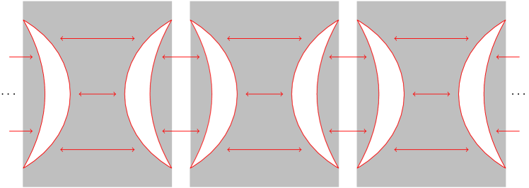
Figure 2: Penrose diagram of the AdS₃ space (in gray) cutoff by UV and IR dS branes (in red). We prepare the state with the Hartle-Hawking construction, considering a thermal density matrix for each brane $\rho_{\rm TFD}$ purified by a maximally entangled partner (UV or IR brane respectively) with an empty bulk in between (white) and glue them together (red arrows), as shown in the figure. Although the UV and IR branes within a single universe are initially unentangled, as the branes accelerate and exchange Hawking modes.

Double holography provides three descriptions of the system:

• $n$ pairs of Euclidean CFT_d-1 defects timelike separated from each pair.

• $n$ double-sided IR and $n$ UV dS_d branes with a matter theory entangled with each other.

• $n$ double-sided AdS_d+1 bulk space cutoff by ETW branes glued along pairs of UV/UV or IR/IR branes periodically.

In the simplest case, $d=2$, gravity would be topological. To study a more dynamical evolution with respect to a braneworld observer, we keep only the tension on the UV branes, and we add an intrinsic gravitational theory, namely JT gravity, on the IR brane. We now analyze the conditions for this configuration to be realized.

UV branes

The theory on the UV braneworlds is given by

$$I_{\text{total}}=I-\mathcal{T}\int_{Q_{c}}\mathrm{d}^{2}x\sqrt{-h}$$ (8)

where $\mathcal{T}$ is the tension of the branes. The brane equation of motion translates to the Israel junction conditions Israel:1966rt

$$\Delta K_{ij}-h_{ij}\Delta K=8\pi G_{3}T_{ij}$$ (9)

where $T_{ij}$ is the effective stress tensor on the brane; $i,\,j$ are $2$-dimensional indices (excluding $\sigma$ components); while $\Delta K_{ij}=K_{ij}^{(+)}-K_{ij}^{(-)}=2K_{ij}^{(+)}$ is the extrinsic curvature difference between opposite sides, denoted by $\pm$, in the double-sided (i.e. the UV and UV, or IR and IR) $Q_{b}$ brane setting.

We consider an outward-directed normal vector $n^{\mu}$, at the location of the $(+)$ side of the UV brane $Q_{c}$. One finds

$$K^{(+)}_{ij}=\tfrac{1}{2}[\partial_{n}h_{ij}]_{\sigma_{c}}=\coth\sigma_{c}\,h_{ij}$$ (10)

where $\partial_{n}=\partial_{\sigma}$. The stress tensor from the brane contribution in (8) then determines the location in terms of the tension of the brane through the relation:

$$\mathcal{T}=\tfrac{1}{4\pi G_{3}}\coth\sigma_{c}\,.$$ (11)

IR branes

Meanwhile, once we include JT gravity as intrinsic theory on the IR branes

$$I_{\text{total}}=I+I_{\text{JT}}$$ (12)

with the JT action given by

$$I_{\text{JT}}=\frac{1}{16\pi G_{\rm JT}}\quantity[\int\mathrm{d}^{2}x\sqrt{-h}\,\Phi_{0}\tilde{\mathcal{R}}+\int\mathrm{d}^{2}x\sqrt{-h}\,\Phi\left(\tilde{\mathcal{R}}-2\Lambda_{\rm JT}\right)]\leavevmode\nobreak\ .$$ (13)

Here, $\Lambda_{\rm JT}$ is the cosmological constant on the brane; $G_{\rm JT}$ is Newton’s gravitational constant on the brane; $\Phi$ is the dilaton, with a topological term $\Phi_{0}$, which we will not consider in the subsequent discussion.

The dilaton equation of motion fixes the background geometry on the ETW brane to be

$$\tilde{\mathcal{R}}=2\Lambda_{\rm JT}\leavevmode\nobreak\ .$$ (14)

Using induced metric at the location of either brane, where $\sigma$ is fixed, (4) with (14) gives

$$\sinh^{2}\sigma_{b}=1/\Lambda_{\rm JT}\leavevmode\nobreak\ ,$$ (15)

which implies that $\Lambda_{\rm JT}$ fixes the brane location, i.e. it plays the role of the brane tension.

On the other hand, one can find the effective stress tensor in the brane with JT gravity by performing the variation of (13) with respect to $h_{ij}$, resulting in the relation:

$$-\nabla_{i}\nabla_{j}\Phi+h_{ij}\nabla^{2}\Phi+h_{ij}\Lambda_{\rm JT}\Phi=8\pi G_{\rm JT}T_{ij}.$$ (16)

Matching (16) and (9) now gives

$$\nabla_{i}\nabla_{j}\Phi+\Lambda_{\rm JT}\Phi h_{ij}=\tfrac{G_{JT}}{G_{3}}\Delta K_{ij}\leavevmode\nobreak\ ,$$ (17)

with the covariant derivative $\nabla_{i}$ taken with respect to the induced metric $h_{ij}$ on the brane.

Next, we look for solutions of the form

$$\Phi=\varphi_{0}+\varphi\leavevmode\nobreak\ ,$$ (18)

with $\varphi$ being the homogeneous solution, i.e.

$$\nabla_{i}\nabla_{j}\varphi+\Lambda_{\rm JT}\,h_{ij}\,\varphi=0\leavevmode\nobreak\ ;$$ (19)

while $\varphi_{0}$ is a constant term, determined as

$$\varphi_{0}=\tfrac{G_{JT}}{2\Lambda_{\rm JT}G_{3}}\Delta K\leavevmode\nobreak\ .$$ (20)

Thus, the junction conditions in ETW branes with JT gravity can be absorbed into an overall constant term in the dilaton on the branes being glued together.

One can find solutions for (19) in global dS₂ coordinates (7)

$$\mathrm{d}s^{2} =\sec^{2}t(-\mathrm{d}t^{2}+\mathrm{d}\alpha^{2})\leavevmode\nobreak\ ,$$ (21)

$$\varphi =\varphi_{1}\tan t+\varphi_{2}\tfrac{\cos\alpha}{\cos t}+\varphi_{0}$$ (22)

with $\varphi_{1}$, $\varphi_{2}$, $\varphi_{0}\in\mathbb{R}$ being constants. We notice that for $\varphi_{1}$, (22) reproduces the dilaton in the full-reduction model dS JT gravity Aalsma:2022swk . It follows that the thermodynamics on the ETW brane also satisfy the relations found for dS JT gravity Svesko:2022txo .

Remark on stability

Although the intrinsic gravity on the branes is decoupled from the ambient AdS₃ gravity as the UV brane is placed at the conformal boundary, small fluctuations of the UV and IR branes could in principle be unstable in this system. To see this, notice that since the IR branes have an opposite orientation with respect to the UV branes, then the extrinsic curvature should be expressed as $K_{ij}=-\coth\sigma_{b}\leavevmode\nobreak\ h_{ij}$, which then implies in (9) that

$$T_{ij}=-\tfrac{1}{4\pi G_{3}}\coth\sigma_{b}h_{ij}.$$ (23)

Since $\sigma_{b}>0$ there would thus be negative components in the stress tensor on the brane, which can then lead to instabilities. In Aguilar-Gutierrez:2023tic a similar type of issue, when the IR brane acquires negative tension, was repaired by making an orbifold projection, such that the unstable mode is eliminated (see also Geng:2022slq ; Geng:2022tfc ). One can repeat the same type of argument in our case. Let the location of the branes fluctuate by allowing: $\sigma_{b}\rightarrow\sigma_{b}+\delta\varphi_{b}$, $\sigma_{c}\rightarrow\sigma_{c}+\delta\varphi_{c}$, where $\delta\varphi_{c,\leavevmode\nobreak\ b}$ represent scalar mode fluctuations. The orbifold projection amounts to setting $\delta\varphi_{b}=0$ so that the unstable mode is eliminated. The effective theory describing the scalar fluctuations in the UV branes then follows similar arguments to Aguilar-Gutierrez:2023tic ; the near boundary effective theory describes scalar fluctuations dS JT gravity as an effective theory. This theory gets increasingly suppressed as the UV brane approaches the AdS boundary. Since our setting also has an independent intrinsic dS JT gravity theory on the IR branes, the action of the system is that of uncoupled dS JT gravity theory on both branes.

3 Coarse-graining of information in the multiverse

In this section, we study the coarse-grained information that can be collected by a UV brane observer in the multiverse model in 2.2 through holographic entanglement entropy and compare it with the von Neumann entropy predicted by the island formula in false vacuum decay models in quantum cosmology Aguilar-Gutierrez:2021bns ; Levine:2022wos .

3.1 Information recovery protocol

our protocol, based on Aguilar-Gutierrez:2023tic , considers an observer collecting Hawking radiation in a single double-sided brane $Q_{c}$, which is close enough to the asymptotic boundary (i.e. $\ell_{d+1}\rightarrow 0$ and $G_{d}\rightarrow 0$), such that the higher curvature corrections can be suppressed. The latter allows us to use the RT formula as well as renders the bath non-gravitating. Gravity decouples and the effective theory of the UV brane is thus described by a dS QFT with a mass gap Maldacena:2012xp ; Fischler:2013fba . We work in the framework of IR/UV entanglement, where, as explained in Balasubramanian:2011wt ; Aguilar-Gutierrez:2023tic , the total Hilbert space factorizes as

$$\mathcal{H}=\mathcal{H}_{\text{UV}}\otimes\mathcal{H}_{\text{IR}}\,,$$ (24)

where $\mathcal{H}_{\text{UV}}$ is the Hilbert space of the dS QFT (with a gap) and $\mathcal{H}_{\text{IR}}$ represents the Hilbert space of the IR degrees of freedom, geometrized by $Q_{b}$. Let $\mathbf{R}$ describe the subregion accessible to the UV observer, such that $\mathbf{R}\subset\partial\hat{\mathcal{M}}$. For simplicity, we will consider an entangling region with disk topology partitioning the $S^{d-1}$ internal space. We thus consider a generic entangling region $\mathbf{R}=I\times S^{d-2}$, with $I=\{\alpha\in[\alpha_{1},\alpha_{2}]\}$. However, given the presence of the JT couplings in the IR brane, the maximal area surfaces do not need to appear at a fixed (global) time (denoted by $\tau$) slice.

In general, if the brane contains an intrinsic gravitational theory, the RT formula describing the von Neumann entropy with respect to a boundary subregion $\mathbf{R}$ can be expressed by,

$$S_{\text{EE}}({\mathbf{R}})=\text{Min}\,\text{Ext}\quantity[\tfrac{A(\Sigma_{\mathbf{R}})}{4G_{d+1}}+\tfrac{A(\sigma_{\mathbf{R}}=\Sigma_{\mathbf{R}}\cap\text{brane})}{4G_{\rm b}}]$$ (25)

where $\Sigma_{\mathbf{R}}$ is the bulk HRT surface (homologous to $\mathbf{R}$), and $\sigma_{\mathbf{R}}$ is its intersection with the brane. The interpretation from the brane perspective is seen as a version of the “island” rule Chen:2020uac ; Chen:2020hmv ; Grimaldi:2022suv .

We now proceed with the evaluation in (25) within a single dS wedge holographic setting, meaning a single AdS₃ space capped off by the UV and IR branes. We evaluate the RT surfaces anchored at the UV brane, whose cutoff surface $\sigma_{c}\rightarrow\infty$ corresponds to $\rho_{c}\rightarrow\infty$.

Our interest is to dress the dS braneworlds with dS JT gravity that models the SdS black hole and generate a braneworld version of the model in Aguilar-Gutierrez:2021bns . We have the option to either add JT gravity on the UV and/or IR branes. In the first case, given that the UV brane represents a weakly gravitating region with Dirichlet boundary conditions, this choice would only amount to a shift in the entropy (35) both before and after the Page transition. Since we are only interested in the entropy difference between the two phases, which is unaffected by adding JT on the UV brane, we will only include JT on the IR brane, which has a nontrivial modification in the variational problem.

We then need to search for minimal-length surfaces, corresponding to the functional

$$S^{\rm bef\,PT}= \frac{1}{4G_{3}}\int_{{\rho}_{t}}^{{\rho}_{c}}\sqrt{1-\cosh^{2}\rho\,\tau^{\prime}({\rho})^{2}+\sinh^{2}{\rho}\,\alpha^{\prime}({\rho})}\leavevmode\nobreak\ \mathrm{d}{\rho}\leavevmode\nobreak\ ,$$ (26)

where $\rho_{t}$ is the turning point, in which $\rho^{\prime}(\alpha)=0$.

Meanwhile, when the RT surfaces land on the IR brane, we consider the entropy functional

$$S^{\rm aft\,PT}= \frac{1}{4G_{3}}\int_{{\rho}_{b}}^{{\rho}_{c}}\sqrt{1-\cosh^{2}\rho\,\tau^{\prime}({\rho})^{2}+\sinh^{2}{\rho}\,\alpha^{\prime}({\rho})}\leavevmode\nobreak\ \mathrm{d}{\rho}+\frac{1}{2G_{\rm b}}\quantity[\varphi_{2}\frac{\cos\alpha_{\rm b}}{\cos t_{\rm b}}+\varphi_{0}]\leavevmode\nobreak\ ,$$ (27)

where the overall factor of $2$ in the contact comes from the two interceptions of the RT on the branes.

3.2 Before the Page transition

We proceed to determine the conserved charges from (26, 27) related to the angular momentum and energy in the ambient AdS₃ space

$$E_{\alpha}=\partialderivative{\mathcal{L}}{\alpha^{\prime}}\leavevmode\nobreak\ ,\quad E_{\tau}=\partialderivative{\mathcal{L}}{\tau^{\prime}}\leavevmode\nobreak\ ,$$ (28)

which allows to solve $\alpha(\rho)$ and $\tau(\rho)$. Since the configuration is empty AdS space and the $Q_{b}$ brane does not play a role before the Page transition, the minimal area surfaces must exist within $\tau=$ constant slices.

For the boundary condition of $\alpha(\rho)$, we take a fixed subregion

$$\alpha(\rho\to\infty)-\alpha_{0}=\Delta\alpha_{c}\leavevmode\nobreak\ ,$$ (29)

from some reference location $\alpha_{0}$. The solution becomes

$$\alpha(\rho)-\alpha_{0}=\arctan{\frac{\sqrt{2}\tan\Delta\alpha_{c}\cosh{\rho}}{\sqrt{\cosh{2\rho}-\sec^{2}\Delta\alpha_{c}}}}\leavevmode\nobreak\ ,$$ (30)

and we can derive that $E_{\alpha}=\tan\Delta\alpha_{c}$. This result allows for the explicit evaluation of (26) as

$$S^{\rm bef\,PT}=\frac{1}{4G_{3}}\int_{\rho_{t}}^{\rho_{c}}\sqrt{1+\alpha^{\prime}(\rho)^{2}\sinh^{2}{\rho}}\leavevmode\nobreak\ \mathrm{d}\rho\leavevmode\nobreak\ ,\\$$ (31)

where there is implicitly some (asymptotic boundary) time dependence via the coordinate map between AdS_d+1 with a dS_d foliation and global AdS_d+1, (6), giving

$$\sinh{\rho_{c}}=\sinh{\sigma_{c}}\cosh{t_{c}}\leavevmode\nobreak\ ,$$ (32)

which grows monotonically with $t_{c}$ as the global dS₂ time with respect to the UV observer (which then grows unbounded). From (29) and (32), we find

$$\rho_{t}=\text{arccosh}(\sec(\Delta\alpha_{c}))\,$$ (33)

where $\Delta\alpha_{c}\in\quantity[-\pi/2,\,\pi/2]$. Then, (31) is just

$$S^{\rm bef\,PT} =\tfrac{1}{4G_{3}}\log\absolutevalue{\frac{\sqrt{\sinh^{2}\sigma_{c}\cosh^{2}t_{c}+1}+\sqrt{\sinh^{2}\sigma_{c}\cosh^{2}t_{c}-\tan^{2}\Delta\alpha_{c}}}{\sec\Delta\alpha_{c}}}\leavevmode\nobreak\ ,$$ (34)

where we employed the map in (6). Notice that this thermal entropy grows monotonically with $t_{c}$ and is unbounded.

In the following, we show that an observer in a given (double-sided) UV braneworld will detect an increase in the von Neumann entropy until reaching a Page transition Aguilar-Gutierrez:2021bns .

3.3 Transition without JT couplings

Given the presence of the IR brane at $\sigma=\sigma_{b}$, there will be a cut-off for the growth in the von Neumann entropy detected by the UV observer. The corresponding entanglement entropy should be evaluated with Neumann boundary conditions on the IR brane, which determines the type of ansatz to be used. Without the JT couplings, one finds a constant entropy from (27), which can be expressed in global dS₂ coordinates as

$$S^{\rm aft\,PT}=\tfrac{1}{2G_{3}}(\sigma_{c}-\sigma_{b})\leavevmode\nobreak\ .$$ (35)

There is an entanglement phase transition between the island (27) and the disconnected phase, which is determined by both $\sigma_{b}$ and $\alpha(\sigma_{c})$. To see that, notice that the disconnected phase in (31) has a minimum at $t=0$, and that when $\sigma_{c}\gg 1$, we get

$$S^{\rm bef\,PT}=\frac{1}{4G_{3}}\quantity(\sigma_{c}-\log\absolutevalue{\sec\Delta\alpha})$$ (36)

Then, comparing with (27), we require

$$\sigma_{b}<\log\absolutevalue{\sec\Delta\alpha}$$ (37)

in order to have a transition. Thus we have an avatar of the picture in Cohen:1998zx relating the UV and IR cutoff of our theory just from the Page curve.

Once can straight-forwardly include boundary time dependence in the previous argument at late times, where $\rho_{c}\simeq\sigma_{c}+t_{c}$. In that case, one finds a Page time at

$$t_{P}=\log\absolutevalue{\sec\Delta\alpha}-\sigma_{b}\leavevmode\nobreak\ .$$ (38)

The result indicates that the time to produce a transition is enhanced by increasing the region where radiation is collected, and there is a threshold given by the location of the IR brane. We then require $\Delta\alpha\simeq\tfrac{\pi}{2}$ for the late time assumption to be valid.

3.4 dS JT gravity on the IR brane

We will now perform the extremization in (27) again, but now the conserved charge $E_{\alpha}$ does not longer vanish at the brane location. We start with the global AdS coordinates (3), with two conserved charges in $d=2$. One can then use the variation of the total action and the solutions to the EOM to evaluate the charge with Neumann boundary conditions. We find,

$$S^{\rm aft\,PT}=\tfrac{1}{2G_{\rm b}}\quantity[\varphi_{1}\tan t_{b}+\varphi_{2}\tfrac{\cos\alpha_{b}}{\cos t_{b}}+\varphi_{0}]+\tfrac{1}{16G_{3}}\log\tfrac{(1+\Delta(\sigma_{c},\,t_{c}))(1-\Delta(\sigma_{b},\,t_{b}))}{(1-\Delta(\sigma_{c},\,t_{c}))(1+\Delta(\sigma_{b},\,t_{b}))}\leavevmode\nobreak\ ,$$ (39)

where

$$\Delta(\sigma,\,t)=\frac{E_{\tau}^{2}-E_{\alpha}^{2}+1+2\sinh^{2}\sigma\cosh^{2}t}{2\sqrt{\left(E_{\tau}^{2}-E_{\alpha}^{2}+1\right)\sinh^{2}\sigma\cosh^{2}t-E_{\alpha}^{2}+\sinh^{4}\sigma\cosh^{4}t}}.$$ (40)

Next, we would like to find out the boundary conditions for the system with JT couplings. For that notice:

$$\delta S^{\rm aft\,PT}= \int_{{\rho}_{b}}^{{\rho}_{c}}\mathrm{d}s\quantity(\partial_{\alpha}\mathcal{L}-\dot{E}_{\alpha}+\partial_{\tau}\mathcal{L}-\dot{E}_{\tau})+\evaluated{E_{\alpha}\delta\alpha}_{{\rho}_{b}}^{{\rho}_{c}}+\evaluated{E_{\tau}\delta{\tau}}_{{\rho}_{b}}^{{\rho}_{c}}$$ (41)

$$+\frac{1}{2G_{\rm b}}\quantity[\varphi_{1}\sec^{2}t_{b}\delta t_{b}+\varphi_{2}\frac{\sin\alpha_{b}}{\cos t_{b}}\delta\alpha_{b}+\varphi_{2}\frac{\cos\alpha_{b}\sin t_{b}}{\cos^{2}t_{b}}\delta t_{b}]\leavevmode\nobreak\ .$$

Imposing Dirichlet boundary conditions at the UV brane gives us

$$\delta\alpha({\rho}_{c})=0,\quad\delta\tau({\rho}_{c})=0\leavevmode\nobreak\ .$$ (42)

Using the map (6) and considering that the location of the branes is fixed (i.e. $\delta\sigma_{\rm brane}=0$); we can deduce the boundary conditions at the location of the IR brane as:

$$\delta t_{b}:\quad E_{\tau}=\frac{1}{2G_{\rm b}}\frac{\tanh^{2}\sigma_{b}\sinh^{2}t_{b}+1}{\tanh\sigma_{b}\cosh t_{b}}\quantity[\varphi_{1}\sec^{2}t_{b}+\varphi_{2}\frac{\cos\alpha_{b}\sin t_{b}}{\cos^{2}t_{b}}],$$ (43)

$$\delta\alpha_{b}:\quad E_{\alpha}=\frac{\varphi_{2}}{2G_{\rm b}}\frac{\sin\alpha_{b}}{\cos t_{b}}\leavevmode\nobreak\ .$$ (44)

We may now evaluate the functional $S^{\rm aft\,PT}$ in (39) subject to (43, 44). However, we need to express $t_{b}$ in terms of the physical parameters measured by the UV observer, namely the angular distance for collecting the radiation $\alpha(\sigma_{c})$, and the physical time $t_{c}$. We will then have to solve the equations of motion of the extremal area surfaces and impose boundary conditions at $\sigma_{c}$, to determine those that minimize $S^{\rm after\leavevmode\nobreak\ PT}$.

Solving the equations of motion resulting from (27) in terms of the conserved charges $E_{\tau}$ and $E_{\alpha}$ in (28) leads to the solution

$$\tan\left(2\left(\alpha(\rho)-\alpha_{0}\right)\right) =\tfrac{\left(1-E_{\alpha}^{2}+E_{\tau}^{2}\right)\sinh^{2}(\rho)-2E_{\alpha}^{2}}{2E_{\alpha}\sqrt{\left(1-E_{\alpha}^{2}+E_{\tau}^{2}\right)\sinh^{2}(\rho)-E_{\alpha}^{2}+\sinh^{4}(\rho)}}$$ (45)

$$\tan\quantity(2(\tau(\rho)-\tau_{0})) =\tfrac{\left(E_{\tau}^{2}-E_{\alpha}^{2}-1\right)\cosh^{2}\rho-2E_{\tau}^{2}}{2E_{\tau}\sqrt{\left(E_{\tau}^{2}-E_{\alpha}^{2}-1\right)\cosh^{2}\rho-E_{\tau}^{2}+\cosh^{4}\rho}}$$ (46)

where $\alpha_{0}$ and $\tau_{0}$ are an arbitrary angular reference point and an arbitrary reference time at which we start measuring the Hawking radiation, respectively.

We may use the transformation to dS global coordinates (7) to express (45) as

$$\tan\left(2\left(\alpha(\sigma)-\alpha_{0}\right)\right)=\tfrac{\left(-E_{\alpha}^{2}+E_{\tau}^{2}+1\right)\sinh^{2}(\sigma)\cosh^{2}(t)-2E_{\alpha}^{2}}{2E_{\alpha}\sqrt{\left(-E_{\alpha}^{2}+E_{\tau}^{2}+1\right)\sinh^{2}(\sigma)\cosh^{2}(t)-E_{\alpha}^{2}+\sinh^{4}(\sigma)\cosh^{4}(t)}}\leavevmode\nobreak\ .$$ (47)

Evaluating (47) at $\sigma_{\rm c}\rightarrow\infty$, we find a relation between the angle measured by the UV observer and the conserved charges:

$$\boxed{2E_{\alpha}\tan(2\Delta\alpha)=-E_{\alpha}^{2}+E_{\tau}^{2}+1}$$ (48)

where $\Delta\alpha=\alpha_{c}-\alpha_{0}$.

Next, we simplify (46) with the dS global coordinates (7):

$$\tanh(2\Delta\tau)=\tfrac{\left(E_{\tau}^{2}-E_{\alpha}^{2}-1\right)\left({\sinh^{2}\sigma\cosh^{2}t}+1\right)-2E_{\tau}^{2}}{2E_{\tau}\sqrt{\left(E_{\tau}^{2}-E_{\alpha}^{2}-1\right)\left({\sinh^{2}\sigma\cosh^{2}t}+1\right)-E_{\tau}^{2}+\left({\sinh^{2}\sigma\cosh^{2}t}+1\right)^{2}}}\leavevmode\nobreak\ .$$ (49)

where $\Delta\tau=\tau(\rho)-\tau_{0}$. At the location of the UV brane, we get

$$\boxed{2E_{\tau}\tanh(2\Delta\tau_{c})=E_{\tau}^{2}-E_{\alpha}^{2}-1\leavevmode\nobreak\ .}$$ (50)

Let us now solve (48, 50) to determine two branches of solutions for $E_{\alpha}$ and $E_{\tau}$:

$$E^{(\pm)}_{\tau}=\tan 2\Delta\tau_{c}\frac{\sec^{2}2\Delta\alpha_{c}\pm{\sec 2\Delta\alpha_{c}\sec 2\Delta\tau_{c}}}{\tan^{2}2\Delta\alpha_{c}-\tan^{2}2\Delta\tau_{c}}\leavevmode\nobreak\ ,$$ (51)

$$E_{\alpha}^{(\pm)}=\frac{\tan 2\Delta\alpha_{c}\sec^{2}2\Delta\tau_{c}\pm{\sec 2\Delta\alpha_{c}\sec 2\Delta\tau_{c}}}{\tan^{2}2\Delta\alpha_{c}-\tan^{2}2\Delta\tau_{c}}\leavevmode\nobreak\ .$$ (52)

Moreover, we have a relation between the charges above with the brane coordinates $t_{b}$, $\alpha_{b}$ in (43, 44), which is enough to determine the solution to the extremization problem.

To solve the above relations we will consider perturbative solutions in $\alpha_{b}\ll 1$, $t_{b}\ll 1$, while keeping $\sigma_{b}$ arbitrary. In that case, combining (43, 44) and taking $\varphi_{1}=0$ gives:

$$t_{b}=\frac{2G_{\rm b}}{\varphi_{2}}\tanh\sigma_{b}E_{\tau}+\mathcal{O}\quantity(\frac{G_{b}^{2}}{\varphi_{2}^{2}})\leavevmode\nobreak\ ,$$ (53)

$$\alpha_{b}=\frac{2G_{\rm b}}{\varphi_{2}}E_{\alpha}+\mathcal{O}\quantity(\frac{G_{\rm b}^{2}}{\varphi_{2}^{2}})\leavevmode\nobreak\ .$$ (54)

Notice that this approximation becomes increasingly better as $\tfrac{\varphi_{2}}{G_{b}}\ll 1$, which corresponds to the semiclassical regime of dS JT gravity.

Using the trigonometric identity

$$\tan\quantity(2(\tau-\tau_{0}))=2\frac{\tan\tau\left(1-\tan^{2}\tau_{0}\right)-\tan\tau_{0}\left(1-\tan^{2}\tau\right)}{{(1-\tan^{2}\tau)(1-\tan^{2}\tau_{0})}+{4\tan\tau_{0}\tan\tau}}\leavevmode\nobreak\ ,$$ (55)

and the map to global dS space coordinates (6), we can express $\Delta\tau_{c}$ purely in terms of $t_{c}$ and $t_{c,\,0}$ (the reference time for the Page curve, at which the UV observer starts collecting the Hawking radiation):

$$\tan 2\Delta\tau_{c}=2\frac{\sinh t_{c}\left(1-\sinh^{2}t_{c,\,0}\right)-\sinh t_{c,\,0}\left(1-\sinh^{2}t_{c}\right)}{{(1-\sinh^{2}t_{c})(1-\sinh^{2}t_{c,\,0})}+{4\sinh t_{c,\,0}\sinh t_{c}}}\leavevmode\nobreak\ .$$ (56)

With all tools at hand, we can evaluate the island transition using (39, 40) as

$$S^{\rm aft\,PT}=\tfrac{1}{2G_{\rm b}}\quantity[\varphi_{2}\tfrac{\cos\alpha_{b}}{\cos t_{b}}+\varphi_{0}]+\tfrac{1}{16G_{3}}\log\absolutevalue{\tfrac{2}{\epsilon_{c}}\tfrac{1-\Delta(\sigma_{b},\,t_{b})}{1+\Delta(\sigma_{b},\,t_{b})}}\leavevmode\nobreak\ ,$$ (57)

where $\epsilon_{c}$ is a UV regulator, and we have set $\varphi_{1}=0$. Since there are 2 roots in (51) and (52), we must explore the one that produces the minimum entropy to identify the island contribution. The comparison between the roots is displayed in Fig. 3, which shows that the dominating saddle is the one determined through $E_{\tau}^{(-)}$, $E_{\alpha}^{(-)}$ in (51, 52). Moreover, one can notice that the entropy for both curves starts decreasing until it reaches an asymptotic late time value, which we deduce below. The decrease in von Neumann entropy can then be used for information recovery using protocols such as Aalsma:2022swk .

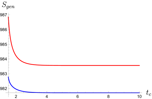
Figure 3: Comparison between $S^{\rm aft\leavevmode\nobreak\ PT}$ (57) for the different root of the conserved charges $E_{\tau}^{(\pm)}$, $E_{\alpha}^{(\pm)}$ in (51) and (52) respectively. The generalized entropy for the $E_{\tau,\,\alpha}^{(-)}$ roots (in blue) dominates over the $E_{\tau,\,\alpha}^{(+)}$ roots (red).

We now deduce the late-time expression for the entropy with the above relations. Using the Ansatz (53, 54), one finds

$$S^{\rm aft\leavevmode\nobreak\ PT}=\tfrac{1}{2G_{b}}(\varphi_{2}+\varphi_{0})+\tfrac{1}{16G_{3}}\log\absolutevalue{\tfrac{2}{\epsilon_{c}}\tfrac{1-\Delta_{b}}{1+\Delta_{b}}}\leavevmode\nobreak\ .$$ (58)

In the limit $t_{c}\gg 1$, we get using (56) that

$$\tan 2\Delta\tau_{c}=\tfrac{2\sinh t_{c,\leavevmode\nobreak\ 0}}{1-\sinh^{2}t_{c,\leavevmode\nobreak\ 0}}\leavevmode\nobreak\ ,$$ (59)

while when $t_{c,\leavevmode\nobreak\ 0}=0$ and $\tau_{c}\rightarrow\infty$, $\Delta\tau_{c}\rightarrow 0$. We therefore have that $\Delta(t_{b},\leavevmode\nobreak\ \sigma_{b})$ in (40) is

$$\Delta(\sigma_{b},\,t_{b})\simeq\frac{E_{\tau}^{2}-E_{\alpha}^{2}+1+2\sinh^{2}\sigma_{b}}{2\sqrt{\left(E_{\tau}^{2}-E_{\alpha}^{2}+1\right)\sinh^{2}\sigma_{b}-E_{\alpha}^{2}+\sinh^{4}\sigma_{b}}}$$ (60)

and it will then become $t_{c}$-independent at late times; thus the von Neumann entropy collected by a UV brane observer at $t_{c}\gg 1$ for generic $\Delta\alpha_{b}$ is just the constant given in (58).

Meanwhile, the late-time asymptotics of the Hawking entropy (34) can be deduced as

$$S^{\rm bef\leavevmode\nobreak\ PT}\simeq\tfrac{1}{4G_{3}}\log\absolutevalue{\tfrac{2}{\epsilon_{c^{\prime}}}\cos\Delta\alpha_{c}\cosh t_{c}}\rightarrow\tfrac{t_{c}}{4G_{3}}\leavevmode\nobreak\ ,$$ (61)

where $\epsilon_{c^{\prime}}$ is a UV regulator when $\sigma_{c}\rightarrow\infty$, and in the last expressing we have discarded $t_{c}$ independent additive terms. The plot of the Page curve, displaying the dominating island and the Hawking phase is shown in Fig. 4.

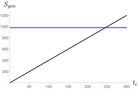
Figure 4: Page curve in a braneworld model with intrinsic dS JT gravity couplings, for a generic choice of parameters. The black curve indicates the Hawking phase $S^{\rm bef\leavevmode\nobreak\ PT}$ (34), and the blue curve $S^{\rm aft\leavevmode\nobreak\ PT}$ (57).

3.5 Central dogma and quantum cosmology interpretation

The previous calculation shows a non-trivial island between the UV and IR branes for a single double-sided UV brane. A natural possibility is to have an island that crosses multiple patches, as shown in Fig. 5 (bottom). In that case, the von Neumann entropy is the $NS^{\rm aft\leavevmode\nobreak\ PT}$ found above, with $N$ the number of patches. The dominating saddle is the one where the island only intercepts the IR brane a single time Fig 5 (top). In contrast, the island saddle encompassing different universes would allow for overlapping HRT surfaces once we introduce another observer on a different double-sided UV brane, shown also in Fig. 5 (bottom). Then, the theory might be in tension with bulk reconstruction, as there would be causally disconnected UV brane observers sharing a common entanglement wedge, corresponding to the bulk AdS space, as this would modify the commutation relations between the observables accessible to the different UV branes.

A similar paradox in the context of dS JT gravity and the connection with the central dogma for cosmological horizons and the no-cloning theorem was discussed in Levine:2022wos , as we mentioned in the introduction.

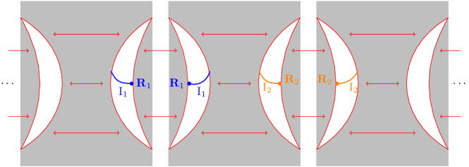
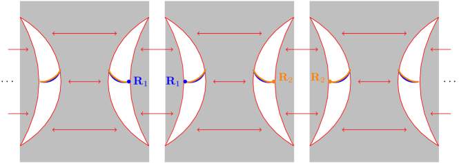
Figure 5: Different island saddles for the multiverse model, where $\mathbf{R}_{1}$ (blue) and $\mathbf{R}_{2}$ (orange) are different UV regions where the observers in each brane universe collect information. Top: Islands ($\mathbf{I}_{1}$, $\mathbf{I}_{2}$ with the same color scheme) connecting a single side of the UV brane to an IR brane, producing the dominant contribution to the entropy (57). Bottom: Island connecting all the universes.

We can view the island transitions in our model through the lenses of quantum cosmology, which shares several similarities to Aguilar-Gutierrez:2021bns ; Levine:2022wos . The information available to a single universe where gravity is non-dynamical (i.e. the UV brane) includes the observers at other universesAguilar-Gutierrez:2021bns . The microscopic degrees of freedom (the UV boundary of AdS₃) can be probed by observers on the UV brane. Yet, the UV observers can only probe the regions available through the islands due to the coarse-graining of information in dS wedge holography, which prohibits communication between observers at different branes.

Then, dS wedge holography provides a conceptually new insight into this problem in the sense that the coarse-graining of information in quantum cosmology, at least for the braneworld multiverse models, involves entanglement between the UV and IR energy modes. It would be of interest to see whether this observation occurs in an explicit model of false vacuum decay in eternal inflation.

4 Discussion

In this work, we have constructed a multiverse toy model based on the dS wedge holography proposal in Aguilar-Gutierrez:2023tic . The multiverse arises by joining, through the Israel junction conditions, an arbitrary number of dS₂ branes cutting off the interior and exterior of AdS₃ space. To have an interesting evolution, while keeping the model exactly solvable, we “dressed” the IR brane as a near Nariai black hole using the dS JT gravity as the intrinsic gravity theory on it. In principle, we could add JT couplings to the UV brane as well, but as we showed this would not qualitatively change our study in any way.

We studied the coarse-graining of information expected in false vacuum eternal inflation Aguilar-Gutierrez:2021bns within our toy model, where a local measurement is coarse-grained over saddle point geometries corresponding to eternal inflation. Similarly, the fine-grained von Neumann entropy (and islands) is determined from the saddle points of the semiclassical path integral. Double holography allowed us to determine the entanglement entropy of Hawking radiation collected by a UV brane observer, which we associated with this coarse-graining, made explicit by the presence of the ETW branes. The appearance of islands connecting the UV and IR modes also allows for a new perspective on this problem.

Having JT gravity on the IR brane has the effect of modifying the Page curve transition and allowing for information recovery with respect to a given dS braneworld observer. Interestingly, we find an avatar of a previous proposal Cohen:1998zx , where a generic effective field theory in curved spacetime is expected to involve a relation between UV and IR cutoffs, in order for consistency relations in the effective field theory description. With our model, one arrives at a similar conclusion, as the Page depends on both UV and IR quantities. In particular, it is bounded from below by the position of the IR brane.

Lastly, the resulting entanglement of Hawking modes captured by a UV brane observer also shows agreement with previous arguments about the central dogma for cosmological horizons and consistency with the no-cloning theorem Levine:2022wos . Namely, there are no overlapping island saddles when we allow for multiple Dirichlet brane observers.

There are some obvious questions to be addressed in the (near) future.

• Most of our work on entanglement in the multiverse model has been focused on the AdS₃ bulk perspective, and made the interpretations with respect to the UV brane observers. However, it would be interesting to have an interpretation of the coarse-graining in quantum cosmology from the time-like separated codimension-2 defects on the interception between the branes for a better understanding, as this might provide a dS/CFT holographic perspective Strominger:2001pn for the coarse-graining of the UV and IR degrees of freedom.

• In the view of describing the coarse-graining of information about gravitational observables in quantum cosmology, and previous work on holographic complexity for dS wedge holography, it could be interesting to study the evolution of gravitational probes in these geometries and compare with the expectations about how their information might be encoded with respect to our findings for holographic entanglement entropy.

• There have been recent discussions about causality violations in braneworlds with an effective theory in the IR brane Neuenfeld:2023svs . It’s unclear how these arguments would be modified for the dS braneworlds, in particular in the presence of JT couplings. However, this could provide a better understanding of when one can trust the effective description of Karch-Randal models in our setup.

• Adding an observer in dS space Chandrasekaran:2022cip ; Witten:2023xze ; Witten:2023qsv ; Aguilar-Gutierrez:2023odp ; Jensen:2023yxy ; Kudler-Flam:2023qfl has led to many developments regarding algebraic studies physical observables and to define generalized entropies. It might be convenient to use these techniques to provide a better understanding of the different entropy transitions found in our work and their connection with coarse-graining in quantum cosmology.

References

- (1) I. Akal, Y. Kusuki, T. Takayanagi and Z. Wei, Codimension two holography for wedges, Phys. Rev. D 102 (2020) 126007 [2007.06800].
- (2) R.-X. Miao, An Exact Construction of Codimension two Holography, JHEP 01 (2021) 150 [2009.06263].
- (3) R.-X. Miao, Codimension-n holography for cones, Phys. Rev. D 104 (2021) 086031 [2101.10031].
- (4) N. Ogawa, T. Takayanagi, T. Tsuda and T. Waki, Wedge Holography in Flat Space and Celestial Holography, 2207.06735.
- (5) A. Bhattacharjee and M. Saha, JT gravity from holographic reduction of 3D asymptotically flat spacetime, JHEP 01 (2023) 138 [2211.13415].
- (6) L. Randall and R. Sundrum, A Large mass hierarchy from a small extra dimension, Phys. Rev. Lett. 83 (1999) 3370 [hep-ph/9905221].
- (7) L. Randall and R. Sundrum, An Alternative to compactification, Phys. Rev. Lett. 83 (1999) 4690 [hep-th/9906064].
- (8) A. Karch and L. Randall, Open and closed string interpretation of SUSY CFT’s on branes with boundaries, JHEP 06 (2001) 063 [hep-th/0105132].
- (9) A. Karch and L. Randall, Locally localized gravity, JHEP 05 (2001) 008 [hep-th/0011156].
- (10) S.B. Giddings, E. Katz and L. Randall, Linearized gravity in brane backgrounds, JHEP 03 (2000) 023 [hep-th/0002091].
- (11) S. Cooper, M. Rozali, B. Swingle, M. Van Raamsdonk, C. Waddell and D. Wakeham, Black hole microstate cosmology, JHEP 07 (2019) 065 [1810.10601].
- (12) Z.-Y. Fan, On holographic braneworld cosmology, 2106.14376.
- (13) S. Antonini and B. Swingle, Cosmology at the end of the world, Nature Phys. 16 (2020) 881 [1907.06667].
- (14) M. Van Raamsdonk, Cosmology from confinement?, JHEP 03 (2022) 039 [2102.05057].
- (15) C. Waddell, Bottom-Up Holographic Models for Cosmology, 2203.03096.
- (16) S. Antonini, P. Simidzija, B. Swingle and M. Van Raamsdonk, Cosmology from the vacuum, 2203.11220.
- (17) S. Antonini, P. Simidzija, B. Swingle and M. Van Raamsdonk, Cosmology as a holographic wormhole, 2206.14821.
- (18) S. Antonini, P. Simidzija, B. Swingle and M. Van Raamsdonk, Can one hear the shape of a wormhole?, 2207.02225.
- (19) S. Antonini, P. Simidzija, B. Swingle, M. Van Raamsdonk and C. Waddell, Accelerating cosmology from gravitational effective field theory, 2212.00050.
- (20) S. Hawking, J.M. Maldacena and A. Strominger, de Sitter entropy, quantum entanglement and AdS / CFT, JHEP 05 (2001) 001 [hep-th/0002145].
- (21) J. Cotler and A. Strominger, The Universe as a Quantum Encoder, 2201.11658.
- (22) R. Emparan, J.F. Pedraza, A. Svesko, M. Tomašević and M.R. Visser, Black holes in dS3, 2207.03302.
- (23) R. Emparan, A.M. Frassino and B. Way, Quantum BTZ black hole, JHEP 11 (2020) 137 [2007.15999].
- (24) C.-S. Chu and H. Parihar, Time-like Entanglement Entropy in AdS/BCFT, 2304.10907.
- (25) S.E. Aguilar-Gutierrez, A.K. Patra and J.F. Pedraza, Entangled universes in dS wedge holography, 2308.05666.
- (26) H. Geng, Y. Nomura and H.-Y. Sun, Information paradox and its resolution in de Sitter holography, Phys. Rev. D 103 (2021) 126004 [2103.07477].
- (27) G. Yadav, Multiverse in Karch-Randall Braneworld, 2301.06151.
- (28) H. Geng, A. Karch, C. Perez-Pardavila, S. Raju, L. Randall, M. Riojas et al., Jackiw-Teitelboim Gravity from the Karch-Randall Braneworld, Phys. Rev. Lett. 129 (2022) 231601 [2206.04695].
- (29) H. Geng, Aspects of AdS2 quantum gravity and the Karch-Randall braneworld, JHEP 09 (2022) 024 [2206.11277].
- (30) H.Z. Chen, R.C. Myers, D. Neuenfeld, I.A. Reyes and J. Sandor, Quantum Extremal Islands Made Easy, Part I: Entanglement on the Brane, JHEP 10 (2020) 166 [2006.04851].
- (31) H.Z. Chen, R.C. Myers, D. Neuenfeld, I.A. Reyes and J. Sandor, Quantum Extremal Islands Made Easy, Part II: Black Holes on the Brane, JHEP 12 (2020) 025 [2010.00018].
- (32) R.-X. Miao, Entanglement island and Page curve in wedge holography, JHEP 03 (2023) 214 [2301.06285].
- (33) D. Li and R.-X. Miao, Massless entanglement islands in cone holography, JHEP 06 (2023) 056 [2303.10958].
- (34) J.H. Lee, D. Neuenfeld and A. Shukla, Bounds on gravitational brane couplings and tomography in AdS3 black hole microstates, JHEP 10 (2022) 139 [2206.06511].
- (35) J. Hartle and T. Hertog, One Bubble to Rule Them All, Phys. Rev. D 95 (2017) 123502 [1604.03580].
- (36) S.E. Aguilar-Gutierrez, A. Chatwin-Davies, T. Hertog, N. Pinzani-Fokeeva and B. Robinson, Islands in Multiverse Models, JHEP 11 (2021) 212 [2108.01278].
- (37) G. Penington, Entanglement Wedge Reconstruction and the Information Paradox, JHEP 09 (2020) 002 [1905.08255].
- (38) A. Almheiri, N. Engelhardt, D. Marolf and H. Maxfield, The entropy of bulk quantum fields and the entanglement wedge of an evaporating black hole, JHEP 12 (2019) 063 [1905.08762].
- (39) S. Ryu and T. Takayanagi, Holographic derivation of entanglement entropy from AdS/CFT, Phys. Rev. Lett. 96 (2006) 181602 [hep-th/0603001].
- (40) S. Ryu and T. Takayanagi, Aspects of Holographic Entanglement Entropy, JHEP 08 (2006) 045 [hep-th/0605073].
- (41) V.E. Hubeny, M. Rangamani and T. Takayanagi, A Covariant holographic entanglement entropy proposal, JHEP 07 (2007) 062 [0705.0016].
- (42) R. Jackiw, Lower dimensional gravity, Nuclear Physics B 252 (1985) 343.
- (43) C. Teitelboim, Gravitation and hamiltonian structure in two spacetime dimensions, Physics Letters B 126 (1983) 41.
- (44) A. Svesko, E. Verheijden, E.P. Verlinde and M.R. Visser, Quasi-local energy and microcanonical entropy in two-dimensional nearly de Sitter gravity, JHEP 08 (2022) 075 [2203.00700].
- (45) A. Levine and E. Shaghoulian, Encoding beyond cosmological horizons in de Sitter JT gravity, 2204.08503.
- (46) V. Pasquarella and F. Quevedo, Vacuum transitions in two-dimensions and their holographic interpretation, JHEP 05 (2023) 192 [2211.07664].
- (47) Y. Iwashita, T. Kobayashi, T. Shiromizu and H. Yoshino, Holographic entanglement entropy of de Sitter braneworld, Phys. Rev. D 74 (2006) 064027 [hep-th/0606027].
- (48) E. Shaghoulian, The central dogma and cosmological horizons, JHEP 01 (2022) 132 [2110.13210].
- (49) J. Garriga, Nucleation rates in flat and curved space, Phys. Rev. D 49 (1994) 6327 [hep-ph/9308280].
- (50) M. Arcos, W. Fischler, J.F. Pedraza and A. Svesko, Membrane nucleation rates from holography, 2207.06447.
- (51) M. Parikh and P. Samantray, Rindler-AdS/CFT, JHEP 10 (2018) 129 [1211.7370].
- (52) W. Israel, Singular hypersurfaces and thin shells in general relativity, Nuovo Cim. B 44S10 (1966) 1.
- (53) L. Aalsma, S.E. Aguilar-Gutierrez and W. Sybesma, An outsider’s perspective on information recovery in de Sitter space, JHEP 01 (2023) 129 [2210.12176].
- (54) J. Maldacena and G.L. Pimentel, Entanglement entropy in de Sitter space, JHEP 02 (2013) 038 [1210.7244].
- (55) W. Fischler, S. Kundu and J.F. Pedraza, Entanglement and out-of-equilibrium dynamics in holographic models of de Sitter QFTs, JHEP 07 (2014) 021 [1311.5519].
- (56) V. Balasubramanian, M.B. McDermott and M. Van Raamsdonk, Momentum-space entanglement and renormalization in quantum field theory, Phys. Rev. D 86 (2012) 045014 [1108.3568].
- (57) G. Grimaldi, J. Hernandez and R.C. Myers, Quantum extremal islands made easy. Part IV. Massive black holes on the brane, JHEP 03 (2022) 136 [2202.00679].
- (58) A.G. Cohen, D.B. Kaplan and A.E. Nelson, Effective field theory, black holes, and the cosmological constant, Phys. Rev. Lett. 82 (1999) 4971 [hep-th/9803132].
- (59) A. Strominger, The dS / CFT correspondence, JHEP 10 (2001) 034 [hep-th/0106113].
- (60) D. Neuenfeld and M. Srivastava, On the Causality Paradox and the Karch-Randall Braneworld as an EFT, 2307.10392.
- (61) V. Chandrasekaran, R. Longo, G. Penington and E. Witten, An Algebra of Observables for de Sitter Space, 2206.10780.
- (62) E. Witten, A Background Independent Algebra in Quantum Gravity, 2308.03663.
- (63) E. Witten, Algebras, Regions, and Observers, 2303.02837.
- (64) S.E. Aguilar-Gutierrez, E. Bahiru and R. Espíndola, The centaur-algebra of observables, 2307.04233.
- (65) K. Jensen, J. Sorce and A. Speranza, Generalized entropy for general subregions in quantum gravity, 2306.01837.
- (66) J. Kudler-Flam, S. Leutheusser and G. Satishchandran, Generalized Black Hole Entropy is von Neumann Entropy, 2309.15897.