Streaming Algorithms for Weighted $k$-Disjoint Matchings

Abstract

We design and implement two single-pass semi-streaming algorithms for the maximum weight $k$-disjoint matching ($k$-DM) problem. Given an integer $k$, the $k$-DM problem is to find $k$ pairwise edge-disjoint matchings such that the sum of the weights of the matchings is maximized. For $k\geq 2$, this problem is NP-hard. Our first algorithm is based on the primal-dual framework of a linear programming relaxation of the problem and is $\frac{1}{3+\varepsilon}$-approximate. We also develop an approximation preserving reduction from $k$-DM to the maximum weight $b$-matching problem. Leveraging this reduction and an existing semi-streaming $b$-matching algorithm, we design a $\frac{k}{(2+\varepsilon)(k+1)}$-approximate semi-streaming algorithm for $k$-DM. For any constant $\varepsilon>0$, both of these algorithms require $O(nk\log_{1+\varepsilon}^{2}n)$ bits of space. To the best of our knowledge, this is the first study of semi-streaming algorithms for the $k$-DM problem.

We compare our two algorithms to state-of-the-art offline algorithms on 82 real-world and synthetic test problems. On the smaller instances, our streaming algorithms used significantly less memory (ranging from 6$\times$ to 114$\times$) and were faster in runtime than the offline algorithms. Our solutions were often within 5% of the best weights from the offline algorithms. On a collection of 6 large graphs with a memory limit of 1 TB and with $k=8$, the offline algorithms terminated only on one graph (mycielskian20). The best offline algorithm on this instance required 640 GB of memory and 20 minutes to complete. In contrast, our slowest streaming algorithm for this instance took under four minutes and produced a matching that was 18% better in weight, using only 1.4 GB of memory.

1 Introduction

Given an undirected weighted graph $G=(V,E,w)$ with $n\coloneqq\left\lvert V\right\rvert$ vertices, $m\coloneqq\left\lvert E\right\rvert$ edges, positive edge weights $w\colon E\to\mathbb{R}_{>0}$, and an integer $k\geq 1$, the $k$-Disjoint Matching ($k$-DM) problem is a generalization of the classical Max Weight Matching (MWM) problem that asks for a maximum weight collection of $k$ pairwise edge-disjoint matchings in $G$. Motivated by applications in reconfigurable datacenter topologies, this NP-hard (for $k\geq 2$) problem was recently studied by Hanauer et al. [19] in the offline setting with the goal of developing fast approximation algorithms. In this work, we develop and implement competitive approximation algorithms for the $k$-DM problem in the single-pass semi-streaming model. In particular, we do so by developing algorithms based on a primal-dual framework and a relaxation to $b$-matchings. To the best of our knowledge, these are the first streaming algorithms for the $k$-DM problem.

Our Contributions

We provide a primal-dual linear programming formulation of the $k$-DM problem and use it to derive a $\frac{1}{3+\varepsilon}$-approximation streaming algorithm that requires $O(nk\log^{2}n)$ bits of space for any constant $\varepsilon>0$ and one pass through the stream, where $n$ is the number of vertices in the graph. The algorithm maintains $k$ stacks, processes the edges as they stream, and employs approximate dual variables to decide which edges should be stored in the $k$ stacks. The number of edges in all the stacks is $O(nk\log n)$.

We also reduce the $k$-DM problem to the well known Max Weight $b$-Matching problem. In particular, we show that any $\alpha$-approximate $b$-matching (with $b=k$) followed by a modified edge coloring algorithm on the $b$-matching subgraph computes an $\frac{\alpha k}{k+1}$-approximate solution for $k$-DM. By plugging in the $\frac{1}{2+\varepsilon}$-approximate semi-streaming $b$-matching algorithm of Huang and Sellier [22], we thus obtain a $\frac{k}{(2+\varepsilon)(k+1)}$-approximate $k$-DM that requires $O(nk\log^{2}n)$ bits of space for any constant $\varepsilon>0$. We note that this reduction is not specific to the semi-streaming setting, and was originally described for unweighted $k$-DM by Feige et al. [11]. Hence, it can be used to develop approximation algorithms for $k$-DM in other computational models where existing $b$-matching results are known.

We implement both algorithms and compare the memory used, running time required, and the weight computed with static offline algorithms designed by Hanauer et al. [19] for this problem. We evaluate the performance of these algorithms on sets of small and large graphs available from the SuiteSparse Matrix Collection [7], as well as a collection of synthetic random graphs. Our results show that the streaming algorithms reduce the memory needed to compute the matchings often by two orders of magnitude and are also faster than the offline static algorithms. Indeed, the latter algorithms do not terminate on all but one of the larger graphs in our test set. The median weights computed by the streaming algorithms are only about $5\%$ lower than the ones obtained by the static algorithms. Among the streaming algorithms, the primal dual algorithm outperforms the $b$-matching-based algorithm in memory needed, time, and weight.

2 Related Work: Streaming Matchings & $k$-DM

In this section we discuss earlier work on matching algorithms in the semi-streaming model and offline $k$-DM algorithms, to put our work in context.

2.1 Semi-Streaming Model

The semi-streaming model [12, 32] was developed to solve massive graph problems where the edges of a graph arrive one by one and the entire graph cannot be stored in memory. For semi-streaming $k$-DM, in a pass, the edges of $E$ are presented one at a time in an arbitrary order. We aim to compute $k$ edge-disjoint matchings in $G$ at the end of the stream, using limited memory and few passes. The semi-streaming algorithm is output-sensitive, i.e., it is allowed to use memory size for processing proportional to the size of the memory needed to store the output. For $k$-DM, the final solution size is $O(nk)$, where $n$ is the number of vertices, and hence the memory limit is $O(nk\cdot\mathrm{polylog}(n))\eqqcolon\tilde{O}(nk)$.

2.1.1 Matchings in the Semi-Streaming Model

Given an undirected graph $G=(V,E,w)$, a matching in $G$ is a subset of edges $M\subseteq E$ such that each vertex is incident to at most one edge in $M$. The weight of a matching $M$ is given by $w(M)\coloneqq\sum_{e\in M}w(e)$. Matching problems are an active area of research in the semi-streaming model. In this model, a common assumption made is that the ratio $W=\frac{w_{\max}}{w_{\min}}$ is $\mathrm{poly}(n)$, where $w_{\max}$ and $w_{\min}$ are the maximum and minimum edge weights, respectively (see [15, 26]). This assumption allows edge weights and their sums to be stored with $O(\log n)$ bits of space.

For arbitrary edge arrivals and in a single pass, Feigenbaum et al. [12] first studied the MWM problem and gave a $\frac{1}{6}$-approximate algorithm. The (worst-case) approximation ratio was subsequently improved by several authors [6, 10, 29, 36]. In a recent breakthrough, Paz and Schwartzman [33] showed that a simple local-ratio algorithm achieves a $\frac{1}{2+\epsilon}$-approximation. Ghaffari and Wajc [15] further simplified their algorithm and provided both a primal-dual and charging based analysis. For arbitrary order streams, this result remains the best known. For random order streams, Gamlath et al. [14] broke the $\frac{1}{2}$-approximation barrier and designed a $(\frac{1}{2}+\epsilon)$-approximate algorithm.

Given a function $b:V\to\mathbb{Z}_{+}$, a $b$-matching in a graph $G$ is a subset $F\subseteq E$ such that at most $b(v)$ edges in $F$ are incident on a vertex $v$. The weight of a $b$-matching $F$ is $w(F)\coloneqq\sum_{e\in F}w(e)$. Levin and Wajc [26] designed a single-pass $\frac{1}{3+\varepsilon}$-approximate streaming algorithm for the Max Weight $b$-Matching (MW$b$-M) problem. The approximation ratio was recently improved to $\frac{1}{2+\varepsilon}$ by Huang and Sellier [22]. The latter algorithm requires $\tilde{O}(|F_{\max}|\log_{1+\varepsilon}(\nicefrac{{W}}{{\varepsilon}}))$ memory, where $F_{\max}$ is a maximum cardinality $b$-matching.

A number of offline approximation algorithms have been designed in recent years for MWM and MW$b$-M, many of which have also been implemented with codes available. Two surveys describing this extensive body of work are found in [21, 34]. These studies show that matching algorithms that employ short augmentations lead to constant factor approximation ratios (e.g., $\frac{1}{2}$, $(\frac{2}{3}-\epsilon)$) and near linear time complexities; practically they are fast and compute solutions with weights a few percentage points off from being optimal, and outperform more involved algorithms with better worst-case approximation ratios (e.g., $(1-\epsilon$)) both in terms of time and matching weight.

2.2 Edge Colorings and Unweighted $k$-DM

The $k$-DM problem is equivalent to a variant of the Edge Coloring problem; in the latter, the goal is to determine the minimum number of colors needed to color the edges of a graph such that neighboring edges receive distinct colors. This number is the chromatic index of a graph. A classical theorem by Vizing [35] states that the chromatic index of any simple graph $G$ is at least $\Delta$ and at most $\Delta+1$, but it is NP-hard to decide between them already for cubic graphs [20]. Hence, most edge coloring algorithms, such as the $O(nm)$ time Misra-Gries algorithm [31], construct $(\Delta+1)$ edge colorings, i.e., colorings that use at most $\Delta+1$ colors.

The $k$-DM problem can be seen as a “maximization” variant of this problem, where given the number of colors $k$ as input, the goal is to find a maximum weight subgraph with chromatic index $k$. A more concrete description of this coloring interpretation is given in Section 3. In the offline setting, unweighted $k$-DM was originally studied in this context by Feige et al. [11], who gave a variety of hardness results and approximation algorithms. For small fixed values of $k$, Kamiński and Kowalik [24] improved on this work and gave algorithms with better approximation ratios. Recently, El-Hayek et al. [9] studied unweighted $k$-DM in the fully dynamic setting and gave algorithms using a black-box reduction to dynamic $b$-matching followed by edge coloring.

2.3 $k$-DM in Reconfigurable Networks in Data Centers

We now discuss an application of matching to design reconfigurable optical networks in data centers.

Network traffic in data centers is growing explosively due to their relevance to data science and machine learning. Since fixed topologies for networks used to route data are oblivious to dynamically changing data traffic, reconfigurable optical technologies offer a promising alternative to existing static network designs. They augment static data center networks with reconfigurable optical matchings, where one edge-disjoint matching is used for each optical circuit switch. Heavy traffic demands (elephant flows) are routed using optical matchings, and the remainder of the traffic (mice flows) is routed on static networks. Thus optical matchings can be adapted to meet dynamic traffic demands and can exploit temporal and spatial structure in the traffic data. Matchings and $b$-matchings in static, online, and dynamic settings (but not in semi-streaming) have been explored in this context in previous work; see among others [1, 2, 3, 30].

Hanauer et al. [19] apply the static $k$-DM problem to reconfigurable data centers with $k$ optical switches. They have shown that the $k$-DM problem is NP-hard and APX-hard, and have developed six offline approximation algorithms, which we describe briefly next.

2.3.1 Offline Approximation Algorithms

Three of these algorithms are based on an iterative matching framework where $k$ matchings are successively computed by running some matching algorithm and removing the matched edges from the graph. Using this framework, variants using the Blossom [8] algorithm, which computes a maximum weight matching, and the Greedy and GPA [28] algorithms, which compute $\frac{1}{2}$-approximate maximum weight matchings, were studied. For the Greedy and GPA variants, they considered post-processing steps using short augmentations such as ROMA [28], and local variations of those augmentations. They also designed a $b$-matching based approach, where they first found a $(k-1)$-matching using a Greedy algorithm and then used the Misra-Gries edge coloring algorithm [31] to construct a $k$-DM. The Blossom variant is shown to be at most $\frac{7}{9}$-approximate and the Greedy variant $\frac{1}{2}$-approximate.

Hanauer et al. [19] also proposed two direct algorithms, NodeCentered and $k$-Edge Coloring, which do not use matching algorithms as a subroutine. The NodeCentered algorithm starts by assigning ratings to vertices, which can be done by taking the sum of the $k$ heaviest edges a vertex is incident on, among other options. Vertices are then processed in rating-decreasing order, and up to $k$ edges a vertex is incident on are colored with any available color in weight-decreasing order. A threshold $\theta\in[0,1]$ is also introduced, which avoids an overly greedy approach by deferring the coloring of edges with weight less than $\theta w_{\max}$. The $k$-Edge Coloring algorithm is an adaption of the Misra-Gries $(\Delta+1)$ edge coloring algorithm [31] that is restricted to using $k$ colors and accounts for edge weights. The iterative GPA, $b$-matching based, NodeCentered, and $k$-Edge Coloring algorithms are shown to be at most $\frac{1}{2}$-approximate through a hypercube graph construction and analyzing the worst-case behavior of these algorithms on the graph. In very recent work [17], some of these algorithms were extended to dynamic and batch-dynamic models.

2.4 Other Applications

Unweighted $k$-DM has been previously studied in [5, 11, 16]. Cockayne et al. [5] motivate unweighted $2$-DM in bipartite graphs with a job assignment problem where a max cardinality 2-disjoint matching implies that on two successive days, maximum assignments can be scheduled such that no person performs the same job twice. This easily generalizes to a weighted setting where the goal is to schedule these disjoint assignments while maximizing some utility. As $k$-DM is related to MW$b$-M (with $b(v)=k$ for all $v\in V$), it is also potentially relevant to applications where $b$-matchings are used, such as graph construction in machine learning [23], load balancing in parallel environments [13], and privacy preservation in datasets [25].

3 Preliminaries

Here we provide formal definitions and concepts needed to describe our streaming algorithms.

3.1 Notation

Consider the graph $G=(V,E,w)$ with weights $w\colon E\mapsto\mathbb{R}_{>0}$. For an edge $e=(u,v)$, we say that $u$ and $v$ are incident on the edge $e$. Given a vertex $v\in V$, we denote by $\delta(v)$ the set of edges $v$ is incident on, and by $\mathrm{deg}(v)\coloneqq\left\lvert\delta(v)\right\rvert$ its degree. The maximum degree of $G$ is $\Delta\coloneqq\max_{v\in V}\mathrm{deg}(v)$. For an edge subset $H\subseteq E$, we let $V(H)$ denote the set of vertices incident on an edge in $H$, and let $G[H]$ denote the subgraph induced by $H$ (i.e., the subgraph whose edge set is $H$ and vertex set is $V(H)$). Likewise, we denote by $\mathrm{deg}_{H}(v)\coloneqq\left\lvert\delta(v)\cap H\right\rvert$ the number of edges in $H$ that a vertex $v\in V$ is incident on and let $\Delta_{H}\coloneqq\max_{v\in V}\mathrm{deg}_{H}(v)$. For a positive integer $t$, we use $[t]$ to represent the set of integers from $1$ to $t$, inclusive. For an integer $s\leq t$, we let $[s..t]$ denote the set of integers from $s$ to $t$, inclusive.

3.2 Problem Definition

Definition 3.1.

Given a graph $G=(V,E,w)$, and an integer $k\geq 1$, a $k$-disjoint matching in $G$ is a collection of $k$ matchings $\mathcal{M}=\{M_{1},\ldots,M_{k}\}$ that are pairwise edge-disjoint (i.e., $M_{i}\cap M_{j}=\emptyset$ for all $i,j\in[k],i\neq j$). The weight of $\mathcal{M}$ is given by $w(\mathcal{M})\coloneqq\sum_{i=1}^{k}w(M_{i})$. The $k$-Disjoint Matching ($k$-DM) problem is to find a $k$-disjoint matching of maximum weight in $G$.

We assume that the ratio $W=\frac{w_{\max}}{w_{\min}}$ is $\mathrm{poly}(n)$, where $w_{\max}=\max_{e\in E}w(e)$ and $w_{\min}=\min_{e\in E}w(e)$. This allows for edge weights and their sums to be stored using $O(\log n)$ bits of space. As in Hanauer et al. [17], we also adopt an edge coloring viewpoint to describe a $k$-disjoint matching. We assume that there is some coloring function $\mathcal{C}\colon E\to[k]\cup\left\{\perp\right\}$ that assigns edges a color from the palette $[k]$ or leaves them uncolored by assigning them the $\perp$ symbol. If $\mathcal{C}$ describes a proper $k$ coloring, where any two adjacent edges $e_{1},e_{2}$ that are colored from the palette $[k]$ satisfy $\mathcal{C}(e_{1})\neq\mathcal{C}(e_{2})$, then it also describes a $k$-disjoint matching. To see this, note that for each color $c\in[k]$, the color class of $c$ (i.e., the set of edges colored with $c$) forms a matching since each vertex $v\in V$ is incident to at most one edge with color $c$. Additionally, each edge is assigned at most one color $c\in[k]$, so none of the color classes share an edge. Thus, the $k$ different color classes form a $k$-disjoint matching.

Theorem 3.2 ([11, 19]).

The $k$-DM problem is NP-hard and APX-hard for $k\geq 2$.

4 A Primal-Dual Approach

We first formulate a linear programming (LP) relaxation of the $k$-DM problem. For each edge $e\in E$ and color $c\in[k]$, we create a variable $x(c,e)$ which is $1$ if $e$ is colored with $c$, and $0$ otherwise. These variables encode the $k$-disjoint matching, i.e., $x(c,e)=1$ implies $e\in M_{c}$. ∑_c ∈[k] ∑_e ∈E w(e) x(c, e)(P) ∑_e ∈δ(v) x(c,e)≤1 ∀v ∈V, c ∈[k] ∑_c ∈[k] x(c,e)≤1 ∀e ∈E x(c, e)≥0 ∀e ∈E, c ∈[k]. The first constraint in the primal LP (P) enforces that $M_{c}$ is a valid matching for each $c\in[k]$, while the second constraint ensures each edge $e\in E$ is colored at most once, and thus belongs to at most one matching $M_{c}$.

For the dual LP (D), we define variables $y(c,v)$ for each color $c\in[k]$ and vertex $v\in V$ and $z(e)$ for each edge $e\in E$. ∑_c ∈[k]∑_v ∈V y(c, v) + ∑_e ∈E z(e)(D) y(c, u) + y(c,v) + z(e)≥w(e) ∀e=(u, v) ∈E, c ∈[k] y(c, v)≥0 ∀v ∈V, c ∈[k] z(e)≥0 ∀e ∈E.

Algorithm 1 Semi-Streaming $k$-DM

1:Input: A stream of edges $E$, an integer $k$, and a constant $\varepsilon>0$

2:Output: A $\frac{1}{3+\varepsilon}$-approximate $k$-disjoint matching $\mathcal{M}$ using $O(nk\log^{2}{n})$ bits of space Initialization

3:$\forall v\in V,\forall c\in[k]:\phi(c,v)\leftarrow 0$

4:$\mathcal{S}\leftarrow\left\{\mathcal{S}_{1},\ldots,\mathcal{S}_{k}\right\}$, where $\mathcal{S}(c)$ is stack $\mathcal{S}_{c}$ Streaming Phase $e=(u,v)\in E$ $c\in[k]$ $w(e)\geq(1+\varepsilon)\left(\phi(c,u)+\phi(c,v)\right)$

5:$w^{\prime}(c,e)\leftarrow w(e)-\left(\phi(c,u)+\phi(c,v)\right)$

6:$\phi(c,u)\leftarrow\phi(c,u)+w^{\prime}(c,e)$

7:$\phi(c,v)\leftarrow\phi(c,v)+w^{\prime}(c,e)$

8:$\mathcal{S}(c)$.push($e$)

9:break Post-Processing

10:$\forall c\in[k]:M_{c}\leftarrow\emptyset$ $c\in[k]$ $\mathcal{S}(c)$ is not empty

11:$e=(u,v)\leftarrow\mathcal{S}(c)$.pop() $V(M_{c})\cap\{u,v\}=\emptyset$

12:$M_{c}\leftarrow M_{c}\cup\{e\}$ $j\in[c+1..k]$ $w(e)\geq(1+\varepsilon)\left(\phi(j,u)+\phi(j,v)\right)$

13:$w^{\prime}(j,e)\leftarrow w(e)-\left(\phi(j,u)+\phi(j,v)\right)$

14:$\phi(j,u)\leftarrow\phi(j,u)+w^{\prime}(j,e)$

15:$\phi(j,v)\leftarrow\phi(j,v)+w^{\prime}(j,e)$

16:$\mathcal{S}(j)$.push($e$)

17:break

18:$\mathcal{M}=\left\{M_{1},\ldots,M_{k}\right\}$

We design a semi-streaming algorithm for $k$-DM in Algorithm 1 based on the primal-dual formulation. For each color $c\in[k]$, it maintains a stack $\mathcal{S}(c)$ in which edges are stored as they stream in and are processed; a matching $M_{c}$ is then computed from each stack $\mathcal{S}(c)$ in a post-processing phase. The algorithm creates approximate dual variables $\phi(c,v)$ for each color $c\in[k]$ and $v\in V$. A parameter $\varepsilon>0$ is used to reduce the space needed for the stacks by constraining edges processed to be sufficiently heavy (relative to the approximate dual variables) before they can be added to a stack, which modifies the approximation ratio of the algorithm.

When the algorithm processes an edge $e=(u,v)$ in the stream, it iterates over the colors $c\in[k]$ to check that it satisfies the condition $w(e)\geq(1+\varepsilon)\left(\phi(c,u)+\phi(c,v)\right)$, If the condition is not satisfied for any color, then the edge is discarded. Otherwise, let $\ell$ be the first color that satisfies it. Then the algorithm computes a reduced weight $w^{\prime}(\ell,e)$ for the edge by subtracting the sum of the approximate dual variables $\phi(\ell,u)$ and $\phi(\ell,v)$ from its weight $w(e)$. The algorithm then pushes the edge into $\mathcal{S}(\ell)$ and updates $\phi(\ell,u)$ and $\phi(\ell,v)$ by the reduced weight $w^{\prime}(\ell,e)$ to reflect the addition of $e$ to the stack $\mathcal{S}(\ell)$.

In the post-processing phase, the matchings $M_{c}$ are constructed from the edges in each stack $\mathcal{S}(c)$. Each stack $\mathcal{S}(c)$ is processed in increasing order of the color $c$, and the edges in each stack are processed in reverse order (i.e., by popping from the stack). For an edge $e=(u,v)$ popped from $\mathcal{S}(c)$, if no earlier popped edge from $\mathcal{S}(c)$ is incident on either $u$ or $v$ in $M_{c}$, then $e$ is added to $M_{c}$. Otherwise, the algorithm checks to see if $e$ can be added to a later stack $\mathcal{S}(j)$ where $j>c$, again based on the condition that $w(e)\geq(1+\varepsilon)\left(\phi(j,u)+\phi(j,v)\right)$. At termination, the algorithm returns a $k$-disjoint matching $\mathcal{M}=\{M_{1},\ldots,M_{k}\}$.

This algorithm generalizes the local-ratio based approach taken by Paz and Schwartzman [33] (and more specifically, the primal-dual interpretation of this algorithm by Ghaffari and Wajc [15]) for the MWM problem to the $k$-DM problem.

4.1 Analysis of the Algorithm

Upon termination of the algorithm, we set the dual variables $y(c,v)=(1+\varepsilon)\phi(c,v)$ for each vertex $v\in V$ and $c\in[k]$. Additionally, we set the dual variable $z(e)$ for each edge $e=(u,v)\in E$ as

$$z(e)=\max_{c\in[k]}\big{\{}\max\left\{w(e)-(1+\varepsilon)\left(\phi(c,u)+\phi(c,v)\right),\;0\right\}\big{\}}\,.$$ (1)

By definition, $z(e)\leq w(e)$. The following claim is immediate from the definition of the dual variables in the LP (D).

Claim 4.1.

For all vertices $v\in V$, edges $e\in E$, and $c\in[k]$, the variables $y(c,v)=(1+\varepsilon)\>\phi(c,v)$ and $z(e)$ computed in Eq. 1 are a feasible solution to (D).

Note that an edge $e$ is attempted to push in a stack $\mathcal{S}(c)$, where $c\in[k]$, at most once (in the line 4 of the streaming or line 12 of the post-processing phase) during the execution of the algorithm. For $c\in[k]$ and an edge $e\in E$, let $\Delta\phi(c,e)$ be the change in the dual variables $\phi$ if it is pushed into the stack $\mathcal{S}(c)$. So, $\Delta\phi(c,e)$ encodes the change in dual variables $\phi$ after inspecting $e$ for stack $c\in[k]$. Formally, let the dual variables on the two endpoints of $e=(u,v)$ be $\phi^{1}(c,u)$ and $\phi^{1}(c,v)$ before inspecting $e$, respectively. Also let $\phi^{2}(c,u)$ and $\phi^{2}(c,v)$ be the corresponding duals after inspecting $e$, then $\Delta\phi(c,e)=\left(\phi^{2}(c,u)+\phi^{2}(c,v)\right)-\left(\phi^{1}(c,u)+\phi^{1}(c,v)\right)$. If $e$ is not pushed into the stack $\mathcal{S}(c)$ (i.e., Conditions in Line  4 or  12 in Algorithm 1 are not satisfied) then, $\Delta\phi(c,e)=0$. We see that when the algorithm terminates for each $c\in[k]$,

$$\sum_{e\in E}\Delta\phi(c,e)=\sum_{v\in V}\phi(c,v).$$ (2)

Also, from lines 6-7 and 14-15 of Algorithm 1 we have that

$$\Delta\phi(c,e)\leq 2w^{\prime}(c,e).$$ (3)

For $c\in[k]$, and an edge $e\in E$, let also $\Delta D(c,e)$ be the total change in the dual that includes the dual variable $z$ too, i.e., $\Delta D(c,e)=\Delta\phi(c,e)+z(e)$. If an edge $e$ is tested for stack $\mathcal{S}(i)$ but is discarded, i.e., the condition on lines 4 and 12 is not true, then $\Delta D(c,e)=0$.

For each edge $e$ added into a stack $\mathcal{S}(c)$, we denote by $\mathcal{P}(c,e)$ the set of preceding adjacent edges (including $e$) added to the same stack no later than $e$. That is,

$$\mathcal{P}(c,e)=\{e^{\prime}\colon e^{\prime}\cap e\neq\emptyset,\;e^{\prime}\textnormal{ is inspected no later than }e\textnormal{ for stack }\mathcal{S}(c)\}.$$ (4)

We now prove the following lemma that connects the weight of an edge with the changes in duals due to the edges processed so far for the corresponding stack.

Lemma 4.2.

For an edge $e$ added to a stack $\mathcal{S}(c)$,

$$w(e)\geq\frac{1}{3}\left(\sum_{e^{\prime}\in\mathcal{P}(c,e)}\Delta\phi(c,e^{\prime})+z(e)\right).$$

Proof.

Recall that, $\Delta\phi(c,e)\leq 2w^{\prime}(c,e)$ (from Eq. 3) and $z(e)\leq w(e)$ (from Eq. 1). Hence, $\Delta D(c,e)\leq 2w^{\prime}(c,e)+w(e)$. For a stack $c\in[k]$, before inspecting $e$, let the values of $\phi(c,u)$ and $\phi(c,v)$ be $\phi^{1}(c,u)$ and $\phi^{1}(c,v)$, respectively. Let us first consider $\phi^{1}(c,u)$. $\phi^{1}(c,u)$ is the accumulation of all the updates $w^{\prime}(c,\{u,x\})=\frac{1}{2}\Delta\phi(c,\{u,x\})$ for some vertex $x$, where the edge $\{u,x\}$ inspected (in the streaming or the post-processing phase) before $e$ for stack $\mathcal{S}(c)$. Hence, $\{u,x\}$ is in $\mathcal{P}(c,e)$. A similar argument also holds for the edges $\{v,x\}$ inspected before $e$, so we get that

$$\phi^{1}(c,u)+\phi^{1}(c,v)\geq\frac{1}{2}\sum_{e^{\prime}\in\mathcal{P}(c,e)\setminus e}\Delta\phi(c,e^{\prime}).$$ (5)

From lines 5 and 13 of Algorithm 1 we obtain

$$w(e) =w^{\prime}(c,e)+\phi^{1}(c,u)+\phi^{1}(c,v)$$

$$\geq\frac{1}{2}(\Delta D(c,e)-w(e))+\frac{1}{2}\sum_{e^{\prime}\in\mathcal{P}(c,e)\setminus e}\Delta\phi(c,e^{\prime}).$$

The inequality follows by using $\Delta D(c,e)\leq 2w^{\prime}(c,e)+w(e)$ and from Eq. 5. Rearranging terms, we get

$$\frac{3}{2}\>w(e) \geq\frac{1}{2}\left(\Delta D(c,e)+\sum_{e^{\prime}\in\mathcal{P}(c,e)\setminus e}\Delta\phi(c,e^{\prime})\right)$$

$$w(e) \geq\frac{1}{3}\left(\Delta D(c,e)+\sum_{e^{\prime}\in\mathcal{P}(c,e)\setminus e}\Delta\phi(c,e^{\prime})\right)$$

$$=\frac{1}{3}\left(\sum_{e^{\prime}\in\mathcal{P}(c,e)}\Delta\phi(c,e^{\prime})+z(e)\right).$$

The equality follows since $\Delta D(c,e)=\Delta\phi(c,e)+z(e)$. ∎

Next, we show that for each color $c\in[k]$ and each edge, $e\in M_{c}$, the corresponding dual value $z(e)$ and the changes of the dual value of $\phi$ encoded by $\Delta\phi(c,e)$ relates to the objective of the Dual LP (D).

Lemma 4.3.

For a color $c\in[k]$, let $M_{c}$ be the final matching then,

$$\sum_{e\in M_{c}}\left(\sum_{e^{\prime}\in\mathcal{P}(c,e)}\Delta\phi(c,e^{\prime})+z(e)\right)=\left(\sum_{v\in V}\phi(c,v)+\sum_{e\in E}z(e)\right)$$

Proof.

Recall that, $z(e)=0$, if $e\notin M_{c}$. The right side of the equality follows from this. For each color, $c\in[k]$, The edge set, $E$ can be partitioned as follows: $E=E_{s}\cup E_{r}$. Here, $E_{s}$ are the edges in the stack $\mathcal{S}(c)$, and $E_{r}$ are the rest of the edges. For an edge, $e$ in $E_{r}$, recall that, $\Delta\phi(c,e)=0$. We will show that upon termination of the algorithm, for each edge, $e$ in $E_{s}$, we account for the corresponding changes, $\Delta(c,e)$ through $\mathcal{P}$. For an edge $e\in E_{s}$, which is also in $M_{c}$, we account for it since, by definition, this edge must be in $\mathcal{P}(c,e)$. Now, think of an edge, $e$, in stack $\mathcal{S}(c)$, but not in $M_{c}$. There must be an edge (say $e^{\prime}$) adjacent to $e\in M_{c}$ that was inspected later than $e$. When we considered $e^{\prime}$, by definition, $e$ was in $\mathcal{P}(c,e^{\prime})$ and thus have already accounted for $\Delta\phi(c,e)$ too. We have,

$$\sum_{e\in M_{c}}\left(\sum_{e^{\prime}\in\mathcal{P}(c,e)}\Delta\phi(c,e^{\prime})+z(e)\right) =\left(\sum_{e\in E}\phi(c,e)+\sum_{e\in E}z(e)\right)$$

$$=\left(\sum_{v\in V}\phi(c,v)+\sum_{e\in E}z(e)\right).$$

The last line follows from Eq. 2. ∎

We are now ready to prove our main results in the following theorem.

Theorem 4.4.

For any constant $\varepsilon>0$, Algorithm 1 is a $\frac{1}{3+\varepsilon}$-approximate semi-streaming algorithm for $k$-DM that uses $O(nk\log^{2}n)$ bits space.

Proof.

Let $\mathcal{M}^{*}$ denote a $k$-disjoint matching of maximum weight, and let $\mathcal{M}=\left\{M_{1},\cdots,M_{k}\right\}$ denote the solution computed by the algorithm. Then

$$w(\mathcal{M}) =\sum_{i=1}^{k}\sum_{e\in M_{i}}w(e)$$

$$\geq\frac{1}{3}\sum_{i=1}^{k}\sum_{e\in M_{i}}\left(\sum_{e^{\prime}\in\mathcal{P}(i,e)}\Delta\phi(i,e^{\prime})+z(e)\right) [\lx@cref{creftype~refnum}{lem:edgeweight}]$$

$$\geq\frac{1}{3}\left(\sum_{i=1}^{k}\sum_{v\in V}\phi(i,v)+\sum_{e\in E}z(e)\right) [\lx@cref{creftype~refnum}{lem:del-phi-dual}]$$

$$\geq\frac{1}{3(1+\epsilon)}\left(\sum_{i=1}^{k}\sum_{v\in V}y(c,v)+\sum_{e\in E}z(e)\right) [y(c,v)=(1+\varepsilon)\>\phi(c,v)]$$

$$\geq\frac{1}{3(1+\epsilon)}w(\mathcal{M}^{*})$$ .

The final inequality from LP duality. The space bound is proved in Lemma B.1 in Appendix B. ∎

The total runtime of Algorithm 1 is $O(km)$, where $m$ is the number of edges in $G$. The processing time for each edge is $O(k)$ as it may be considered for insertion into each of the $k$ stacks. Additionally, the size of each stack is trivially bounded by $m$, so the post-processing step of unwinding the stacks takes $O(km)$ time.

5 A $b$-Matching Based Approach

Recall that a $b$-matching generalizes a matching by allowing each vertex to be incident to at most $b(v)$ matched edges for some function $b\colon V\to\mathbb{Z}_{+}$. When $b(v)=k$ for all $v\in V$, where $k$ is some positive integer, we refer to the matching as a $k$-matching and consider the Max Weight $k$-Matching (MW$k$-M) problem.

It is important to note that MW$k$-M is different from $k$-DM. In the former, a feasible solution is a subgraph with maximum degree at most $k$, while in the latter a feasible solution is a subgraph that can be covered by $k$ pairwise disjoint matchings. A simple example of this difference is given by the triangle graph $K_{3}$, where a $2$-matching can contain all three edges, but a $2$-disjoint matching consists of at most two edges, with each edge constituting a matching.

It is easy to see that every $k$-disjoint matching also induces a valid $k$-matching, but the reverse need not hold. Thus, a $k$-matching relaxes the notion of a $k$-disjoint matching and MW$k$-M is a relaxation of $k$-DM (i.e. if $F^{\ast}$ and $\mathcal{M}^{\ast}$ are optimal solutions to MW$k$-M and $k$-DM on the same graph, respectively, then $w(F^{\ast})\geq w(\mathcal{M}^{\ast})$). This leads to a simple approach to approximately solve $k$-DM, which is to first solve MW$k$-M and then modify the resulting $k$-matching into a feasible $k$-disjoint matching. More specifically, we can

1. Solve MW$k$-M, which gives a $k$-matching $F$.

2. Properly $(\Delta_{F}+1)$ color the edges of the subgraph induced by $F$, which may use up to $k+1$ colors.

3. Return $\mathcal{M}$, the collection of edges colored by the $k$ heaviest color classes.

This is the same approach Feige et al. [11] use to develop a $\frac{k}{k+1}$-approximation algorithm for unweighted $k$-DM. In the following lemma, we extend this result to general $k$-DM and also show that this transformation is approximation preserving.

Lemma 5.1.

Let $F$ be an $\alpha$-approximate solution to MW$k$-M on a graph $G$. If the induced subgraph $G[F]$ is properly $(\Delta_{F}+1)$ colored, the collection of edges colored by the $k$ heaviest color classes gives an $\frac{\alpha k}{k+1}$-approximate solution to $k$-DM on $G$.

Proof.

Let $\mathcal{M}$ represent a solution to $k$-DM on $G$. Additionally, let $F^{\ast}$ and $\mathcal{M}^{\ast}$ be the optimal solutions to MW$k$-M and $k$-DM on $G$, respectively.

By definition of a $k$-matching, we have that $\Delta_{F}\leq k$. If $\Delta_{F}<k$, then the edge coloring used at most $k$ colors and we can simply let $\mathcal{M}=\left\{M_{1},\ldots,M_{k}\right\}$, where $M_{i}$ is the set of edges colored with $i$ for $i\in[k]$. Note that in this case, $w(\mathcal{M})=w(F)$. Otherwise, if $\Delta_{F}=k$ then the edge coloring may have used $k+1$ colors. Without loss of generality, let $k+1$ be the color class with the minimum weight. Again let $\mathcal{M}=\left\{M_{1},\ldots,M_{k}\right\}$, where $M_{i}$ is the set of edges with color $i$ for $i\in[k]$. Note that by discarding the edges with color $k+1$, at most a $\frac{1}{k+1}$ fraction of the weight of $F$ is lost. Thus, in either case

$$w(\mathcal{M})\geq\frac{k}{k+1}w(F)\geq\frac{\alpha k}{k+1}w(F^{\ast})\geq\frac{\alpha k}{k+1}w(\mathcal{M}^{\ast}),$$

where the penultimate inequality follows from the definition of $F$, and the last inequality follows from MW$k$-M being a relaxation of $k$-DM. ∎

Note that properly $(\Delta+1)$ coloring a graph $H$ can be done in $O(|E_{H}|)$ space using the $O(|E_{H}||V_{H}|)$ time Misra-Gries algorithm [31]. If we use a semi-streaming algorithm for MW$k$-M to handle the streaming process and find some $k$-matching $F$, the remaining post-processing steps of the algorithm only require memory linear in $\left\lvert F\right\rvert$. Thus, we get a trivial semi-streaming algorithm for $k$-DM. Using the basic semi-streaming $\frac{1}{2+\varepsilon}$-approximation algorithm of Huang and Sellier [22] for MW$b$-M with $b(v)=k$ for all $v\in V$, which for any constant $\varepsilon>0$ requires $O(nk\log^{2}n)$ space, Lemma 5.1 implies a semi-streaming $\frac{k}{(2+\varepsilon)(k+1)}$-approximation algorithm for $k$-DM using the same space. We formalize this approach in Algorithm 2, where we use Stream-$b$M and Color to refer to the algorithms of Huang and Sellier [22] and Misra and Gries [31], respectively.

Algorithm 2 Semi-Streaming $k$-DM via MW$k$-M

1:Input: A stream of edges $E$, an integer $k$, and a constant $\varepsilon>0$

2:Output: A $\frac{k}{(2+\varepsilon)(k+1)}$-approximate $k$-disjoint matching $\mathcal{M}$ using $O(nk\log^{2}n)$ bits of space Initialization

3:$\forall v\in V\colon b(v)\leftarrow k$ Streaming Phase

4:$F\leftarrow$ Stream-$b$M$E$, $b$, $\frac{\varepsilon}{2}$ $\triangleright$ MW$k$-M solution Post-Processing

5:$\Delta_{F}\leftarrow\max_{v\in V}\mathrm{deg}_{F}(v)$ $\triangleright$ $\Delta_{F}\leq k$

6:Color$G[F]$ $\triangleright$ Uses colors $\left\{1,\ldots,\Delta_{F}+1\right\}$ $\Delta_{F}+1=k+1$

7:WLOG let $k+1$ denote the color class with the lowest weight

8:$\forall i\in[k]\colon M_{i}\leftarrow\left\{e\in F\colon\mathcal{C}(e)=i\right\}$

9:$\mathcal{M}=\left\{M_{1},\ldots,M_{k}\right\}$

Theorem 5.2.

For any constant $\varepsilon>0$, Algorithm 2 is a $\frac{k}{(2+\varepsilon)(k+1)}$-approximate semi-streaming algorithm for $k$-DM that uses $O(nk\log^{2}n)$ space.

The total runtime of Algorithm 2 is $O(km+kn^{2})$. The streaming phase requires $O(k)$ processing time per incoming edge while constructing the resulting $k$-matching $F$ trivially takes $O(m)$ time. By definition of a $k$-matching, the size of $\left\lvert F\right\rvert$ is bounded by $O(kn)$, so the post-processing coloring step requires $O(kn^{2})$ time.

6 Heuristic Improvements

In this section, we describe some heuristics we employ to speed up and improve the weight of both of the streaming algorithms we have presented.

6.1 Dynamic Programming (DP) Based Weight Improvement

Manne and Halappanavar [27] proposed a general scheme to enhance the weight of matchings. Consider two edge disjoint matchings $M_{1}$ and $M_{2}$. It can easily be seen that the subgraph $G[M_{1}\cup M_{2}]$ only contains paths or even length cycles. Utilizing a linear time dynamic programming based strategy, an optimal matching $M^{\prime}$ can be derived on $G[M_{1}\cup M_{2}]$. The weight of $M^{\prime}$ is only guaranteed to be at least as large as $\max\left\{w(M_{1}),w(M_{2})\right\}$, but in practice this heuristic results in substantially improved weight.

We further adapt this method for the algorithm described in Section 4 in the following way: instead of computing a $k$-disjoint matching, we first compute a $2k$-disjoint matching. These $2k$ matchings are then merged into $k$ disjoint ones. While various strategies can be used for this merging process, we merge the $i$-th matching with the $(2k-i+1)$-th matching, for $i\in[k]$. Note that this approach does not alter the asymptotic memory or runtime complexities for streaming algorithms since each merge requires additional $O(n)$ time and space.

6.2 Common Color and Merge

For the $b$-matching based approach we use two heuristics. The first is the common color heuristic described by Hanauer et al. [19], which attempts to color an edge by first determining if there is a common free color on both of its endpoints instead of going through the Misra-Gries routine. The second is the merge heuristic, which is used when the number of color classes is $k+1$ and tries to improve the solution weight by merging the lowest and second lowest weight color classes instead of completely discarding the lowest weight one. This is done through the dynamic programming routine previously described.

7 Experiments and Results

This section reports experimental results for several real-world and synthetic graphs. All of the tested algorithms were executed on a node of a community cluster computer with 128 cores in the node, where the node is an AMD EPYC 7662 with 1 TB of total memory over all the cores. The machine has three levels of cache memory. The L1 data and instruction caches, the L2 cache, and the L3 cache have 4 MB, 32 MB, and 256 MB of memory, respectively. The page size of the node is 4 KB.

Our streaming algorithms are implemented using C++17 and compiled with g++9.3.0 using the -O3 optimization flag. The streaming algorithms are simulated by sequentially reading edges from a graph file using the C++ fstream class and processing the edge. We compare them against several offline algorithms in the DJ-Match software suite [18] developed by Hanauer et al. [19]. All the streaming and offline algorithms are sequential, and the runtimes reported for these algorithms do not include file reading times. For computing the memory consumed by the program, we use the getrusage system call to retrieve the maximum resident set size (RSS) during the program’s execution.

7.1 Datasets and Benchmark Algorithms

Our testbed consists of three datasets. Following [19, 25], we include ten weighted graphs from the Suitesparse Matrix Collection [7] that we label as SuiteSmall. These instances are generated from diverse applications such as collaboration networks, medical science, structural mechanics, and random networks. Similar to [19], we also generated 66 synthetic instances, which we label as Rmat, using the R-MAT model [4] with $2^{x}$ vertices, where $x\in[10..20]$. We used three initiator matrices, $\mathsf{rmat_{\text{b}}}=(0.55,0.15,0.15,0.15)$, $\mathsf{rmat_{\text{g}}}=(0.45,0.15,0.15,0.25)$, and $\mathsf{rmat_{\text{er}}}=(0.25,0.25,0.25,0.25)$. For each of the three types, we assign real-valued weights from the range $[1,2^{19}]$ according to uniform or exponential distributions. Unfortunately, we could not include the data center traffic problems from [19] in our test set since the data was currently not available on the Web (personal communication). However, these are smaller graphs than the ones we discuss next. Our final dataset (SuiteLarge) consists of six of the largest undirected graphs in the Suitesparse Matrix Collection [7], with each graph having more than 1 billion edges. For three unweighted graphs (mycielskian20, com-Friendster, Agatha_2015), we assign uniform random real weights in the range $[1,10^{6}]$. In Appendix A, we list statistics on the graphs in the SuiteLarge and SuiteSmall collections in Tables 3(b) and 3(a), respectively, while the statistics of the Rmat instances are given in Table 4.

We summarize the algorithms we compare in Table 1. It was concluded in [19] that four of the offline algorithms were the most practical in terms of runtime and solution quality. These include the iterative greedy algorithm (Greedy-It), the iterative Global Paths Algorithm (GPA-It), the NodeCentered algorithm (NC), and the $k$-Edge Coloring algorithm (k-EC) that we described in more detail in Section 2. For these four offline algorithms, we use the heuristics and post-processing steps recommended in [19], which we list in Table 1. Due to space considerations, we refer to [19] for a detailed description of these heuristics.

Algorithm	Heuristics	Approx.	Time Complexity
Greedy-It	LS	$\nicefrac{{1}}{{2}}$	$O(\textrm{srt}(m)+km)$
GPA-It	LS	$\leq\nicefrac{{1}}{{2}}$	$O(\textrm{srt}(m)+km)$
NC	$\theta=0.2$, Agg=sum	$\leq\nicefrac{{1}}{{2}}$	$O(\textrm{srt}(n)+n\cdot\textrm{srt}(\Delta)+km)$
k-EC	CC-RL	$\leq\nicefrac{{1}}{{2}}$	$O(\textrm{srt}(m)+kn^{2})$
stk / stk-dp		$\frac{1}{3+\epsilon}$	$O(km)$
stkb	CC-M	$\frac{k}{(2+\varepsilon)(k+1)}$	$O(km+kn^{2})$

Table 1: Benchmark approximation algorithms. LS: Local swaps, CC: Common color, RL: Rotate long, M: Merge, Agg: Aggregation, $\text{srt}(x)$: Time complexity of sorting $x$ elements. The parameter $\theta$ is discussed in Sec. 2.

7.2 Comparison of Streaming Algorithms

We first compare six variants of our streaming algorithms among themselves. For the primal-dual based approach, we include the standard stk algorithm and the stk-dp variant (Section 6.1). For the $b$-matching based approach, we have the CC (common color) and M (merge) heuristics in addition to the standard stkb algorithm, for a total of four different combinations.

In Fig. 1, we show the relative quality results on SuiteSmall for the streaming algorithms. We set $\epsilon=0.001$ and tested with $k\in\left\{2,4,8,16,32,64,96\right\}$, but observed that beyond $k=32$, all the algorithms computed similar weights, since, at this point, the solutions likely contain nearly the entire graph. Hence, we only report results up to $k=32$. For each graph, algorithm, and $k$ value combination, we conduct five runs and record the mean runtime, memory usage, and solution weight. We calculate relative time by taking the ratio of the mean runtime for each algorithm to the mean runtime of a baseline algorithm. Relative memory and relative weight are similarly computed. We choose stk as the baseline algorithm for runtime and memory comparisons and stk-dp as the baseline for weight comparisons. We show geometric means of the relative time and relative memory of the algorithms across the graphs against $k$ values in Fig. 1 (a) and (b), respectively. For the weights, we show the box plot of the relative weights across all the graphs and $k$ value combinations in Fig. 1 (c).

For runtimes, we see that the fastest algorithm is stk, while the slowest are stkb and stkb-m. stkb-cc and stkb-cc-m both have similar runtimes and are faster than stkb and stkb-m. The runtime of stk-dp is between stk and stkb-cc-m. In terms of memory usage, stk requires the least, while stk-dp requires roughly twice ($1.76$-$1.86\times$ across $k$) its memory on average. The other four $b$-matching based algorithms behave similarly to each other and are worse than both stk and stk-dp. For weights, the relative weight of stk-dp is always one, so we did not show it in the plot. In terms of median relative weight (the orange line), stk is the second best, and stkb-cc-m is the third best. Surprisingly, while the worst-case approximation guarantee of the primal-dual based approach is weaker than the $b$-matching based approaches, it provides weights that are better than the latter in nearly all instances.

From this experiment, we conclude that among these six streaming algorithm variants, the best three are stk, stk-dp, and stkb-cc-m. Hence all the remaining experiments will report results only for these three versions of the streaming algorithms.

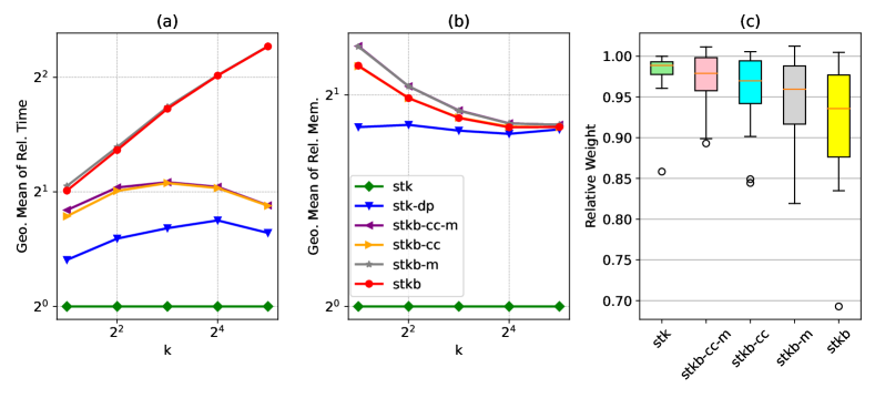
Figure 1: Summary plots for SuiteSmall instances on different streaming algorithms with $\varepsilon=0.001$. (a) Geometric mean of relative time and (b) geometric mean of relative memory across all instances with increasing $k$ values. (c) Boxplot of relative weights across all instances and $k$ values for each algorithm. The baseline algorithms for each metric are listed in the text. Note the logarithmic scales of the axes in the first two subplots.

7.3 Comparison with Offline Algorithms

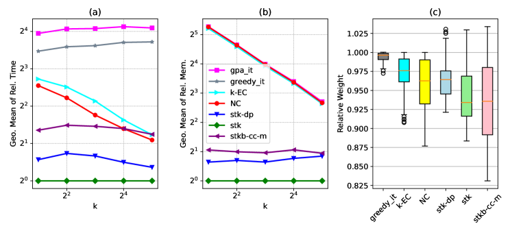
Figure 4: Summary plots for the streaming and offline algorithms on Rmat. (a) Geometric mean of relative time and (b) geometric mean of relative memory, across all instances with increasing $k$ values. (c) Boxplot of relative weights across all instances and $k$ values for each algorithm. We set $\epsilon=0.001$ for stk, stk-dp and stkb-cc-m. The baseline algorithms are same as the SuiteSmall experiment, and note the logarithmic scales in the axes of the first two subplots.

Next, we compare the three streaming algorithms with the four offline algorithms listed in Table 1. We show the relative runtime, memory, and weight plots for the algorithms for the SuiteSmall and Rmat datasets in Fig. 2 and Fig. 4 (in Appendix A), respectively. We follow the experimental settings and computations as in Section 7.2 with baseline algorithms chosen as follows. The stk algorithm was chosen as the baseline for relative time and memory experiments, and GPA-It with local swaps as the baseline algorithm for weight results, since generally these are the best performers for the three metrics.

We first discuss the SuiteSmall results. All of the streaming algorithms are significantly faster than the offline ones. The fastest among these is the stk algorithm, while the slowest is the $b$-matching based stkb-cc-m. Among the offline algorithms, GPA-It is the slowest, more than $20\times$ slower in geometric mean than stk, while Greedy-It is more than $15\times$ slower. The other two algorithms are relatively faster with similar runtimes but still slower than all streaming algorithms. The speedup for stk w.r.t to NC and k-EC ranges from 3 to 11 across $k$. As an example, for $k=8$, both NC and k-EC are more than $6\times$ slower than stk. We also observe that both NC and k-EC get relatively more efficient as $k$ increases, which was also reported in [19]. For the memory results, we see that stk requires the least, while the other two streaming algorithms take almost twice the memory, on average. All the offline algorithms behave similarly in terms of memory consumption since they all need to store the entire graph, which dominates the total memory consumption. We see a substantial memory reduction when using the streaming algorithms, with improvement ranging from 114$\times$ to 11$\times$ in geometric mean across $k$. For smaller value of $k$ this reduction is more pronounced.

We now focus on the case $k=8$. All the streaming algorithms consume at least 16$\times$ less memory than the offline algorithms, while for stk it is $32\times$. For the largest graph (kron_g500-logn21) in this set, we see all the offline algorithms require at least 45 GB of memory while the streaming algorithms consume less than 1GB of memory. We emphasize that the higher memory requirement of the offline algorithms prohibits them from being run on larger datasets, as we will see later. While the streaming algorithms are very efficient in terms of memory and time, we also see they obtain reasonably high solution weights. For the quality results, we set GPA-It as the baseline algorithm; hence, we do not include it in the box plot. All the offline algorithms find heavier weights than the streaming algorithms; for the NC and k-EC algorithms, we see many outliers compared to the other algorithms. Among the streaming algorithms, stk-dp obtains the heaviest weight, with only less than 4% median deviation from the best weight. For stk-dp, the geometric mean of relative weights is 0.96 at $k=2$ and improves to 0.97 at $k=32$. The corresponding geometric mean of relative weights for faster offline algorithms, NC and k-EC are as follows: for $k=2$, the means are 0.96 and 0.97, respectively, and for $k=32$, they are 0.97 and 0.98, respectively. This highlights stk-dp’s comparable quality to the closest practical offline alternatives. The stk and stkb-cc-m algorithms compute weights where the median deviation from the best weight is less than 5% and 6%, respectively.

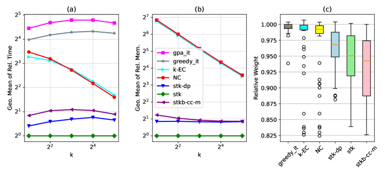
Figure 2: Summary plots the streaming and offline algorithms on SuiteSmall. (a) Geometric mean of relative time and (b) geometric mean of relative memory across all instances with increasing $k$ values. (c) Boxplot of relative weights across all instances and $k$ values for each algorithm. We set $\epsilon=0.001$ for stk, stk-dp and stkb-cc-m. Again, the baseline algorithms are listed in the text, and note the logarithmic scales in the axes of the first two subplots.

We repeat similar experiments with the Rmat dataset and show the results in Fig. 4 in Appendix A. Overall, a similar conclusion can be drawn as the SuiteSmall instances. The random graphs generated are much smaller than the SuiteSmall instances, which explains the smaller memory improvement (6$\times$ to 38$\times$ in Geo. mean) obtained by the streaming algorithms. For the Rmat instances, the streaming algorithms obtain better quality results than the SuiteSmall instances. The difference between the streaming and the NC and k-EC algorithms is smaller than seen in the SuiteSmall instances. Both NC and stk-dp achieve similar relative weights, while k-EC is marginally (within 1%) better.

Finally, we visualize the performance of these algorithms on SuiteSmall using a $3$D plot in Fig. 3. The three axes are the geometric mean of relative time, relative memory, and relative weight across all the graphs. For each algorithm, we have five points (denoted by filled circles in the plot) representing the $k$ values from $2$ to $32$. Larger $k$ values are denoted by larger circles. The algorithms fall into three separate clusters. The top cluster represents the Greedy-It and GPA-It algorithms, which provide the best weights but require high amounts of time and memory. In the middle region are the NC and k-EC algorithms that do not achieve as high weights but are faster. Finally, we have the streaming algorithms, which are more efficient in terms of memory and runtime, but have slightly lower weights (lower Geo. mean of relative weights by at most $7\%$). The stk-dp streaming algorithm achieves the highest weights while stkb-cc-m often has the lowest weight.

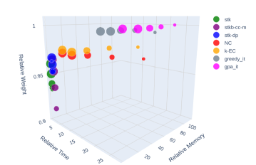
Figure 3: 3D plot of the geometric mean of relative time, memory, and weights for different algorithms across SuiteSmall graphs for different $k$ values. Larger $k$ values are illustrated by circles of larger radii.

7.4 SuiteLarge Graph Results

	stk			stk-dp			stkb-cc-m
Graph	Time (s)	Weight	Mem (GB)	Rel. Time	% Wt. Imprv.	Rel. Mem.	Rel. Time	% Wt. Imprv.	Rel. Mem.
AGATHA_2015	1377.54	1.60e+14	49.41	1.64	0.67	1.90	0.99	-1.51	1.69
MOLIERE_2016	736.75	8.26e+6	23.28	1.64	2.03	1.78	1.48	0.26	1.22
GAP-kron	629.37	1.20e+10	29.66	1.85	3.05	1.90	1.06	-0.46	1.62
GAP-urand	679.73	9.83e+10	53.25	1.67	3.71	1.57	2.11	-1.30	1.75
com-Friendster	475.13	1.02e+14	22.66	1.62	2.84	1.81	1.49	-4.58	1.54
mycielskian20	86.14	1.99e+12	0.65	2.34	5.30	2.17	0.98	-10.10	1.03

Table 2: Comparison of streaming algorithms for $k=8$ and $\epsilon=0.001$ on SuiteLarge graphs.

Our final experiment consists of six large graphs from the Suitesparse Matrix Collection [7]. Since these graphs require longer runtimes, and our experiments on the smaller graphs reveal little deviation in runtime and memory across runs (the weight remains constant as our algorithms are deterministic), we report in Table 2 the results of a single run of our streaming algorithms. We chose $k=8$ and set $\varepsilon=0.001$ for this experiment. The first three columns represent the time in seconds, weight, and memory in GB for the baseline stk algorithm, while the next six columns represent the relative metrics for the stk-dp and stkb-cc-m algorithms. For all the instances, using stk-dp yields an increase in solution quality over stk, with the average increase being 2.93%. Consistent with the results on smaller graphs, stkb-cc-m obtains the lowest weight among the streaming algorithms with weight decreasing in almost all the instances compared to stk and the average decrease is 2.95%. In terms of memory and runtime, stk-dp and stkb-cc-m require at most twice as much memory and time as the stk algorithm. The geometric mean of relative memory and runtime of stk-dp is 1.85 and 1.78, respectively, and for stkb-cc-m they are 1.45 and 1.30, respectively.

For the offline algorithms, we chose to test with the NC and k-EC algorithms since the prior experiments show they have much lower runtimes than the other two iterative matching algorithms. These algorithms were only able to be run on the smallest graph in this dataset (mycielskian20) while respecting the $1$ TB memory limit. For this graph, k-EC and NC obtained weights of 1.70e+12 and 1.68e+12, respectively, which are around $18\%$ less than stk-dp. The k-EC algorithm required more than two hours to compute a solution, while NC required about twenty minutes. This is much worse than any of the streaming algorithms, as even the slowest one (stk-dp) required less than four minutes. Both the NC and k-EC algorithms used around 640 GB of memory, while the memory usage of the streaming algorithms ranges from $660$ MB for stk to $1.4$ GB for stk-dp, which provides at least a $450$-fold reduction.

8 Conclusions and Future Work

Earlier work on offline maximum weight matching algorithms showed that exact algorithms run out of memory and do not terminate on graphs with hundreds of millions of edges. Hence offline approximation algorithms with near-linear time complexities based on short augmentations were designed [34]. However, our results show that on graphs with billions of edges, even these algorithms require over $1$ TB of memory for the $k$-DM problem, and do not terminate on such graphs.

The primary objective of streaming algorithms is to reduce the memory requirements and our streaming $k$-DM algorithms are effective in reducing it by one to two orders of magnitude on our test set. Our results also show that the streaming algorithms are theoretically and empirically faster. In particular, we conclude that the stk-dp algorithm is the best performer since it only requires modestly more memory and runtime than the stk algorithm while still computing solutions comparable (within 4%) to the best offline algorithm.

We also find that stk consistently outperforms stkb-cc-m in weight, despite its weaker worst-case approximation ratio. While such results have been seen for maximum weight matching problems in earlier work, it also raises the question of whether the approximation ratio of stk could be improved to $\frac{1}{2+\varepsilon}$.

As for reconfigurable network problems in data centers, dynamic matchings responsive to time-varying demands are necessary. In recent work, Hanauer et al. [17] designed several dynamic and batch-dynamic algorithms for $k$-DM using three offline algorithms. Since the transformation from $k$-DM to $b$-matching developed in this work is also approximation preserving and does not rely on the computational model, we may use existing dynamic weighted $b$-matching algorithms to design dynamic $k$-DM algorithms, as was done recently in the unweighted case by El-Hayek et al. [9]. We leave it as a future work to explore this connection further.

Appendix A Additional Experimental Details

Graph	$n$	$m$	Avg. Deg.	Max. Deg.	Min. Deg.
mycielskian20 (U)	786.43 K	1.36 B	3446.42	393,215	19
com-Friendster (U)	65.61 M	1.81 B	55.06	5,214	1
GAP-kron (W)	134.22 M	2.11 B	31.47	1,572,838	0
GAP-urand (W)	134.22 M	2.15 B	32	68	6
MOLIERE_2016 (W)	30.24 M	3.34 B	220.81	2,106,904	0
Agatha_2015 (U)	183.96 M	5.79 B	62.99	12,642,631	1

(a) SuiteLarge graph instances. U: Unweighted, W: Weighted Graph.

Graph	$n$	$m$	Avg. Deg.	Max. Deg.	Min. Deg.
astro-ph	16,706	121,251	14.52	360	0
Reuters911	13,332	148,038	22.21	2,265	0
cond-mat-2005	40,421	175,691	8.69	278	0
gas_sensor	66,917	818,224	24.45	32	7
turon_m	189,924	778,531	8.20	10	1
Fault_639	638,802	13,303,571	41.65	266	0
mouse_ gene	45,101	14,461,095	641.27	8,031	0
bone010	986,703	23,432,540	47.50	62	11
dielFil.V3real	1,102,824	44,101,598	79.98	269	8
kron.logn21	2,097,152	91,040,932	86.82	213,904	0

(b) SuiteSmall graph instances. All the graphs are weighted.

Table 3: Graph statistics for SuiteLarge and SuiteSmall instances.

	$\mathsf{rmat_{\text{b}}}$			$\mathsf{rmat_{\text{g}}}$			$\mathsf{rmat_{\text{er}}}$
$\log n$	$m$	Avg. Deg.	$\Delta$	$m$	Avg Deg.	$\Delta$	$m$	Avg Deg.	$\Delta$
10	7,939	15.51	372	7,960	15.55	85	8,185	15.99	28
11	16,025	15.65	615	16,030	15.65	120	16,377	15.99	31
12	32,302	15.77	864	32,282	15.76	171	32,761	15.99	34
13	64,917	15.85	1,280	64,884	15.84	160	65,531	15.99	35
14	130,214	15.90	1,700	130,169	15.90	199	131,067	15.99	35
15	260,905	15.92	2,502	260,886	15.92	261	262,133	15.99	35
16	522,434	15.94	3,471	522,451	15.94	276	524,273	15.99	34
17	1,046,118	15.96	5,085	1,045,962	15.96	416	1,048,561	15.99	36
18	2,093,484	15.97	7,029	2,093,526	15.97	465	2,097,142	15.99	41
19	4,189,181	15.98	10,222	4,189,155	15.98	606	4,194,296	15.99	38
20	8,381,379	15.99	14,374	8,381,431	15.99	644	8,388,594	15.99	37

Table 4: Number of edges $m$, average and maximum degrees ($\Delta$) for the R-MAT graphs generated for each scale $x\in[10..20]$ and initiator matrix.

Appendix B Omitted Proofs

B.1 Space Bound of Algorithm 1

Lemma B.1.

For any constant $\varepsilon>0$, Algorithm 1 uses $O(nk\log^{2}n)$ bits of space.

Proof.

Consider any vertex $v\in V$ and color $c\in[k]$. Let $e=(u,v)$ be an edge that is pushed to stack $\mathcal{S}(c)$, and let $\phi^{\text{old}}(c,\cdot)$ and $\phi^{\text{new}}(c,\cdot)$ be the values of $\phi(c,\cdot)$ before and after it is pushed to the stack, respectively. Note that since $e$ is pushed to $\mathcal{S}(c)$, it must be that $w(e)\geq(1+\varepsilon)\phi^{\text{old}}(c,e)$. Then,

$$\phi^{\text{new}}(c,v)-\phi^{\text{old}}(c,v) =w(e)-\phi^{\text{old}}(c,e)$$

$$\geq(1+\varepsilon)\phi^{\text{old}}(c,e)-\phi^{\text{old}}(c,e)$$

$$\geq\varepsilon\phi^{\text{old}}(c,v)$$

$$\phi^{\text{new}}(c,v) \geq(1+\varepsilon)\phi^{\text{old}}(c,v).$$

Hence, adding an edge to $\mathcal{S}(c)$ that $v$ is incident on increases $\phi(c,v)$ by at least a $(1+\varepsilon)$ factor. If $e$ is the first edge that $v$ is incident on that is added to stack $\mathcal{S}(c)$, then $\phi^{\text{old}}(c,v)=0$, and

$$\phi^{\text{new}}(c,v) =w(e)-\phi^{\text{old}}(c,e)$$

$$\geq w(e)-\frac{w(e)}{1+\varepsilon}\geq\frac{\varepsilon}{1+\varepsilon}w_{\min}.$$

Thus the minimum non-zero value of $\phi(c,v)$ is $\frac{\varepsilon}{1+\varepsilon}w_{\min}$. On the other hand, the maximum value of $\phi(c,v)$ is easily given by $w_{\max}$. Recall, $W=\frac{w_{max}}{w_{min}}.$Thus, $\phi(c,v)$ can increase at most $\log_{1+\varepsilon}(\nicefrac{{W}}{{\varepsilon}})+1$ times. Hence at most $\log_{1+\varepsilon}(\nicefrac{{W}}{{\varepsilon}})+1$ edges in $\delta(v)$ can be pushed to $\mathcal{S}(c)$. Hence, the size of $\mathcal{S}(c)$ is bounded by $O(n\log n)$ (since we assume $\varepsilon$ is constant and $W$ is $\mathrm{poly}(n)$) and the total number of edges stored among all the stacks is at most $O(nk\log n)$. Each edge can be represented with $O(\log n)$ bits for a total space requirement of $O(nk\log^{2}n)$ for the edges. Furthermore, each variable $\phi(\cdot,\cdot)$ only requires $O(\log n)$ space to be stored as it is essentially just the sum of edge weights, and hence it takes $O(nk\log n)$ space in total to store all of them. ∎

References

- [1] Hitesh Ballani, Paolo Costa, Raphael Behrendt, Daniel Cletheroe, Istvan Haller, Krzysztof Jozwik, Fotini Karinou, Sophie Lange, Kai Shi, Benn Thomsen, and Hugh Williams. Sirius: A flat datacenter network with nanosecond optical switching. In Proc. of the 2020 Conference of the ACM Special Interest Group on Data Communication (SIGCOMM 2020), pages 782–797, 2020. doi:10.1145/3387514.3406221.
- [2] Marcin Bienkowski, David Fuchssteiner, Jan Marcinkowski, and Stefan Schmid. Online dynamic -matching: With applications to reconfigurable datacenter networks. SIGMETRICS Performance Evaluation Review, 48(3):99–108, 2021. doi:10.1145/3453953.3453976.
- [3] Marcin Bienkowski, David Fuchssteiner, and Stefan Schmid. Online -matchings for reconfigurable datacenters: The power of randomization. arXiv preprint arXiv:2209.01863, 2022. doi:10.48550/arXiv.2209.0186.
- [4] Deepayan Chakrabarti, Yiping Zhan, and Christos Faloutsos. R-MAT: A recursive model for graph mining. In Proc. of the 2004 SIAM International Conference on Data Mining (SDM 2004), pages 442–446, 2004. doi:10.1137/1.9781611972740.43.
- [5] Ernest J. Cockayne, Bert L. Hartnell, and Stephen T. Hedetniemi. A linear algorithm for disjoint matchings in trees. Discrete Mathematics, 21(2):129–136, 1978. doi:10.1016/0012-365X(78)90085-7.
- [6] Michael S. Crouch and Daniel M. Stubbs. Improved streaming algorithms for weighted matching, via unweighted matching. In Proc. of the 17th International Workshop on Approximation Algorithms for Combinatorial Optimization Problems (APPROX 2014), pages 96–104, 2014. doi:10.4230/LIPIcs.APPROX-RANDOM.2014.96.
- [7] Timothy A. Davis and Yifan Hu. The University of Florida Sparse Matrix Collection. ACM Transactions on Mathematical Software, 38(1), 2011. doi:10.1145/2049662.2049663.
- [8] Jack Edmonds. Paths, trees, and flowers. Canadian Journal of Mathematics, 17:449–467, 1965. doi:10.4153/CJM-1965-045-4.
- [9] Antoine El-Hayek, Kathrin Hanauer, and Monika Henzinger. On -matching and fully-dynamic maximum -edge coloring. 2023. arXiv:2310.01149, doi:10.48550/arXiv.2310.01149.
- [10] Leah Epstein, Asaf Levin, Julián Mestre, and Danny Segev. Improved approximation guarantees for weighted matching in the semi-streaming model. SIAM Journal on Discrete Mathematics, 25(3):1251–1265, 2011. doi:10.1137/100801901.
- [11] Uriel Feige, Eran Ofek, and Udi Wieder. Approximating maximum edge coloring in multigraphs. In Proc. of the 5th International Workshop on Approximation Algorithms for Combinatorial Optimization Problems (APPROX 2002), pages 108–121, 2002. doi:10.1007/3-540-45753-4_11.
- [12] Joan Feigenbaum, Sampath Kannan, Andrew McGregor, Siddharth Suri, and Jian Zhang. On graph problems in a semi-streaming model. Theoretical Computer Science, 348(2-3):207–216, 2005. doi:10.1016/j.tcs.2005.09.013.
- [13] SM Ferdous, Alex Pothen, Arif Khan, Ajay Panyala, and Mahantesh Halappanavar. A parallel approximation algorithm for maximizing submodular -matching. In Proc. of the 2021 SIAM Conference on Applied and Computational Discrete Algorithms (ACDA21), pages 45–56, 2021. doi:10.1137/1.9781611976830.5.
- [14] Buddhima Gamlath, Sagar Kale, Slobodan Mitrovic, and Ola Svensson. Weighted matchings via unweighted augmentations. In Proc. of the 2019 ACM Symposium on Principles of Distributed Computing (PODC 2019), pages 491–500, 2019. doi:10.1145/3293611.3331603.
- [15] Mohsen Ghaffari and David Wajc. Simplified and space-optimal semi-streaming (2+)-approximate matching. In Proc. of the 2nd Symposium on Simplicity in Algorithms (SOSA 2019), pages 13:1–13:8, 2019. doi:10.4230/OASIcs.SOSA.2019.13.
- [16] Branko Grünbaum. Matchings in polytopal graphs. Networks, 4(2):175–190, 1974. doi:10.1002/net.3230040207.
- [17] Kathrin Hanauer, Monika Henzinger, Lara Ost, and Stefan Schmid. Dynamic demand-aware link scheduling for reconfigurable datacenters. In Proc. of the 42nd IEEE Conference on Computer Communications (INFOCOM 2023), 2023. doi:10.48550/arXiv.2301.05751.
- [18] Kathrin Hanauer, Monika Henzinger, Stefan Schmid, and Jonathan Trummer. DJ-Match/DJ-Match: Version 1.0.0, Jan 2022. doi:10.5281/zenodo.5851268.
- [19] Kathrin Hanauer, Monika Henzinger, Stefan Schmid, and Jonathan Trummer. Fast and heavy disjoint weighted matchings for demand-aware datacenter topologies. In Proc. of the 41st IEEE Conference on Computer Communications (INFOCOM 2022), pages 1649–1658, 2022. doi:10.1109/INFOCOM48880.2022.9796921.
- [20] Ian Holyer. The NP-Completeness of edge-coloring. SIAM Journal on Computing, 10(4):718–720, 1981. doi:10.1137/0210055.
- [21] Stefan Hougardy. Linear time approximation algorithms for degree constrained subgraph problems. In William Cook, László Lovász, and Jens Vygen, editors, Research Trends in Combinatorial Optimization, pages 185–200. Springer Verlag, 2009. doi:10.1007/978-3-540-76796-1_9.
- [22] Chien-Chung Huang and François Sellier. Semi-streaming algorithms for submodular function maximization under -matching constraint. In Proc. of the 24th International Conference on Approximation Algorithms for Combinatorial Optimization Problems (APPROX 2021), pages 14:1–14:18, 2021. doi:10.4230/LIPIcs.APPROX/RANDOM.2021.14.
- [23] Tony Jebara, Jun Wang, and Shih-Fu Chang. Graph construction and -matching for semi-supervised learning. In Proc. of the 26th Annual International Conference on Machine Learning (ICML 2009), pages 441–448, 2009. doi:10.1145/1553374.1553432.
- [24] Marcin Kamiński and Łukasz Kowalik. Beyond the Vizing’s bound for at most seven colors. SIAM Journal on Discrete Mathematics, 28(3):1334–1362, 2014. doi:10.1137/120899765.
- [25] Arif Khan, Krzysztof Choromanski, Alex Pothen, S. M. Ferdous, Mahantesh Halappanavar, and Antonino Tumeo. Adaptive anonymization of data using -edge cover. In Proc. of the 2018 International Conference for High Performance Computing, Networking, Storage, and Analysis (SC 2018), pages 59:1–59:11, 2018. doi:10.1109/SC.2018.00062.
- [26] Roie Levin and David Wajc. Streaming submodular matching meets the primal-dual method. In Proc. of the 32nd ACM-SIAM Symposium on Discrete Algorithms (SODA 2021), pages 1914–1933, 2021. doi:10.1137/1.9781611976465.114.
- [27] Fredrik Manne and Mahantesh Halappanavar. New effective multithreaded matching algorithms. In Proc. of the 2014 IEEE 28th International Parallel and Distributed Processing Symposium (IPDPS 2014), pages 519–528, 2014. doi:10.1109/IPDPS.2014.61.
- [28] Jens Maue and Peter Sanders. Engineering algorithms for approximate weighted matching. In Proc. of the 6th International Conference on Experimental Algorithms (WEA 2007), pages 242–255, 2007. doi:10.1007/978-3-540-72845-0_19.
- [29] Andrew McGregor. Finding graph matchings in data streams. In Proc. of the 8th International Workshop on Approximation Algorithms for Combinatorial Optimization Problems (APPROX 2005), pages 170–181, 2005. doi:10.1007/11538462\_15.
- [30] William M. Mellette, Rob McGuinness, Arjun Roy, Alex Forencich, George Papen, Alex C. Snoeren, and George Porter. Rotornet: A scalable, low-complexity, optical datacenter network. In Proc. of the 2017 Conference of the ACM Special Interest Group on Data Communication (SIGCOMM 2017), pages 267–280, 2017. doi:10.1145/3098822.3098838.
- [31] Jayadev Misra and David Gries. A constructive proof of Vizing’s Theorem. Information Processing Letters, 41(3):131–133, 1992. doi:10.1016/0020-0190(92)90041-S.
- [32] S. Muthukrishnan. Data streams: Algorithms and applications. Foundations and Trends in Theoretical Computer Science, 1(2):117–236, 2005. doi:10.1561/0400000002.
- [33] Ami Paz and Gregory Schwartzman. A (2+)-approximation for maximum weight matching in the semi-streaming model. ACM Transactions on Algorithms, 15(2):18:1–18:15, 2019. doi:10.1145/3274668.
- [34] Alex Pothen, SM Ferdous, and Fredrik Manne. Approximation algorithms in combinatorial scientific computing. Acta Numerica, 28:541–633, 2019. doi:10.1017/S0962492919000035.
- [35] Vadim G. Vizing. The chromatic class of a multigraph. Cybernetics, 1(3):32–41, 1965. doi:10.1007/BF01885700.
- [36] Mariano Zelke. Weighted matching in the semi-streaming model. Algorithmica, 62(1-2):1–20, 2012. doi:10.1007/s00453-010-9438-5.