Response to referee report for MN-23-2373-MJ

We acknowledge the referee for their report. To keep track of all the comments, we have constructed this document to hold the full discussion history for specific points, colour-coded for clarity.

As usual, we have highlighted any change in the manuscript using a bold font.

 

1 B.0 Abstract

Referee. Accurately encompasses precisely.

Response. Accurately does not encompass precisely; a measurement can be accurate but lack precision, and vice-versa.

Referee. You speak about A-type stars, but the reported effective temperatures indicate an early F-type.

Response. The components are F-type and this mistake has been corrected.

Referee. Were all data sets used?

Response. Information regarding which data sets were used is too much information for an abstract. This information is given in the observations section.

Referee. Cooler, but more massive secondary: what is the implication in terms of stellar evolution.

Response. We have revised the sentence as follows: ”cooler, but larger and more massive than the primary so is more evolved”. Any more information than this would again be too much information for the abstract.

Referee. Misses relevant information, e.g. tidal perturbations of some frequencies: what kind of “perturbations” for which kind of frequencies?

Response. Tidally perturbed frequencies are a subclass of tidally split modes; they can be either tidally tilted or tidally perturbed, so stating they are tidally perturbed is sufficient. To address which kind of frequencies are tidally perturbed, we have revised the sentence as follows: ”We find evidence for tidal perturbations to some of the p- and g-modes.”

Referee. Misses relevant information; buoyancy radius and near-core rotation: for which component?

Response. Agreed. We clarify that these measurements are made for the primary component in the revised sentence.

Referee. Regarding the age: Is it consistent with the previous information about the secondary component.

Response. Yes, given that a single isochrone of this age is able to predict the corresponding observed properties of both components. The corresponding evolutionary tracks also show the secondary to be approaching the TAMS, so our observations of the secondary are expected for our new age of 1.259 Gyr. This is too much information for the abstract.

 

2 B.1 Introduction

Referee. Regarding medium- and -high mass stars: Specify mass range.

Response. Mass range has been specified in the revised text.

Referee. Precise ”best”!

Response. Revised sentence: ”best source of precise fundamental stellar parameters.”

Referee. Which measurements?

Response. We have specified which measurements in the revised sentence.

Referee. Precise or accurate, what do you mean?

Response. We mean precise here. This is because evolutionary status and age determinations are based on theoretical models. Thus, precise and accurate measurements for the masses and radii lead to a precisely isolated location in stellar models, but the accuracy of the corresponding age and evolutionary stage estimate depends on the accuracy of the models.

Referee. Precise vs accurate

Response. Accurate may be a better word to use regarding the seismic measurements. The precision of seismic measurements is probably, in general, less precise than those from EBs. However, seismic measurements are considered accurate. Thus, we have replaced ”precisely” with ”accurate” in the revised text here.

Referee. which system? This could make the link toward asteroseismology (see above paragraph that appears suddenly).

Response. We have updated the citation to include which system it is referring to. We have also taken the advice to put this sentence at the start of the preceding paragraph so it appears less ”suddenly”.

Referee. Reposition the references appropriately in the sentence, reading is uneasy.

Response. We have repositioned the references.

Referee. Where/when is this difficult? Reposition the references in the sentence.

Response. Using the word ”where” is probably not appropriate. The word ”which” would have been better, so have used it instead. One reference remains in the same position but have now indicated that it is an example, other reference positioned at end of sentence.

Referee. Not very precise.

Response. The new sentence states the location of the $\gamma$ Doradus instability strip more precisely.

Referee. About space missions, why is it relevant here? Put it in Observations (Sect. 2).

Response. It is relevant here because it is the unprecedented precision and continuous monitoring of stars provided by space missions that has allowed for the discovery of so many hybrid pulsators. We want to make this point in the introduction whilst introducing hybrids since it is important.

Referee. There is no mention that this is not confirmed theoretically!!

Response. Hybrids were expected to be rare based on calculations by Dupret et al. (2005) but modern calculations by Xiong et al. (2016) conform better with the discovery that hybrids are common. We discuss these points in the revised text.

Referee. And not only the ones in the overlap region where they are expected…

Response. We confirm this comment in the original sentence since we refer to ”all” $\delta$  Scuti stars.

Referee. You might include a reference.

Response. Reference included.

Referee. In conclusion.

Response. Agreed; starting the sentence with ”In conclusion” would improve the flow here. However, we have chosen to go with ”Therefore”.

Referee. The results by Guo et al. (2016) should be mentioned somewhere in detail. This study is very relevant for the present conclusions.

Response. We have included more details about the study by Guo et al. (2016).

Referee. What kind of study is this?

Response. We have revised the sentence to state clearly the kind of study being referred to.

Referee. Needs to be decoupled and detailed more.

Response. We have done this in the revised version of the paragraph.

Referee. Although very extensive, this section reads with much difficulty. The writing style is without transition in-between the paragraphs that do not appear to follow any scheme and come without warning. The presence of many references also breaks the fluency of reading. The section furthermore lacks precision in some formulations. E.g. the acronym ‘EBs’ $\to$ Do you mean ‘SB2 eclipsing binaries’ (everywhere from hereon) or just ‘eclipsing binaries’?

Response. We have followed the advice in the annotated version of the pdf. We think that the modifications made based on addressing those comments satisfies the overall points made here.

 

3 B2 Observations

3.1 B.2.1 Photometry

Referee. Mention the six quarters.

Response. We have addressed this comment by giving the six quarters.

Referee. Same as above?

Response. The sentence being referred to is indeed similar to the sentence describing that Kepler has provided a huge amount of data on stars and stellar systems. Hence, in the sentence being referred to, which is describing the TESS mission, we include the word ”also”. The point is that TESS has ”also” provided a large amount of data on other celestial objects. Modifications here are not necessary.

Referee. Any reference here? What was done to these data?
Specify what happened with these data or how they differ from the SAP data.

Response. A brief description is provided for the Kepler and TESS data with a reference for the Kepler data (Jenkins 2017) and TESS data (Jenkins et al. 2016). The difference between the SAP and PDCSAP data is given, further processing is carried out on the latter compared to the former.

Referee. Was this verified and if it the case, what happens to the eclipse depths?

Response. To verify this, we normalise the light curves by dividing them by their median flux value, without performing any other processing, simply to put the two sets of flux measurements on the same scale; the raw light curves are shifted relative to each other in the vertical direction due to the extra processing that is applied to the PDCSAP fluxes. Fig.1 shows the SAP light curves with the PDCSAP light curves overplotted, demonstrating the similarity of the light curves. The eclipse depths are clearly comparable.

We have made mention of this inspection in the main text.

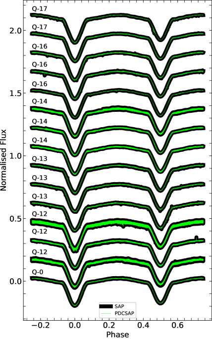
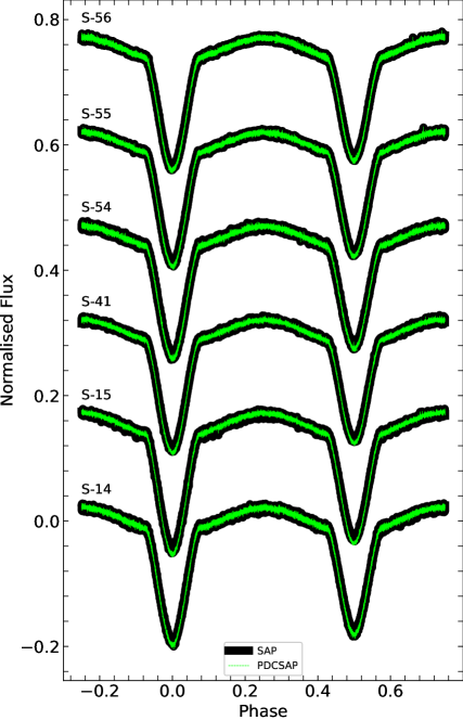
Figure 1: SAP fluxes (black) with PDCSAP fluxes (green) over-plotted as a function of orbital phase. Left; Kepler light curves. Right; TESS light curves. Corresponding quarters and sectors are given.

Referee. How low?

Response. The revised text specifies that a second order polynomial was used.

Referee. How was this defined with the bow shape of the out-of-eclipse data? Which parts of the light curve were used to define this median level?

Response. We have modified the description to give a more details of the operation being referred to: A second-order polynomial was fitted to fluxes that correspond to positions of quadrature, i.e., the maximum of the ellipsoidal brightening, to estimate systematic trends present in the light curves. Subtracting the difference between this polynomial and the median flux of the light curve yields a model for the local median level of out-of-eclipse flux. This model was then divided out to remove systematic trends as well as normalize the light curves.

Referee. Is this the smoothening as explained before?

Response. This comment is confusing since no smoothing has been reported prior to the statement that the comment is referring to.

Referee. What is it??

Response. We have rephrased the sentence being referred to so that it is more clear.

Referee. This paragraph mixes information about the Kepler and TESS data, and shows only the Kepler light curve as an example (quarter 0). What is the quality of the other light curves, in particular the quality and contribution of the ground-based data?
Although all are mentioned, I could not find one TESS neither one WASP light curve displayed. Were these data used? If yes, where and for which aim?
Specify the units! Caption: Which light curve, original or processed?

Response. Information about the Kepler and TESS missions is given in two separate paragraphs. The detrending and normalization is not explained separately because the procedures are the same for both Kepler and TESS light curves.

We have updated Fig.1 to show an example of a Kepler and TESS light curve as well as a cuts of the WASP light curve phase folded about the orbital period. The units are specified as BJD-2400000 for the x-axis of the top two panels and phase for the bottom panels. Differential magnitude is the unit of the y-axis for all panels.

What the Kepler and TESS light curves are used for is now stated clearly. The use of the WASP data, simply to constrain the times primary minima in the preliminary fits to the Kepler and TESS light curves, is also made clear.

3.2 B.2.2 Spectroscopy

Referee. Contains minimal information. Lacks the essential information, precision and an illustration of the quality of the obtained spectra, e.g. a mean (general) S/N? Where is the logbook of the collected spectra with their individual (BJD) epochs and individual properties such as S/N?

Response. We provide a Table containing the epochs for each spectral observations, corresponding RVs of the components, as well as S/N for each spectral estimated as the square root of the maximum counts in each case.

Referee. Were the spectra normalized? If yes, how was it done?

Response. Normalization was carried out differently to extract RVs and to perform SPD. The description for how the spectra were normalized to extract RVs was already given. For the SPD section, we provide the following details:
Basic outline of procedure used in normalisation and merging echelle orders is given. Reference to procedure used is given (Kolbas 2015), in particular concerning normalisation of echelle orders containg broad Balmer lines (later used as primary indicator of the effective temperatures). Also, references of recent application of our procedure is given.

We have also directed the reader to these details in the current section.

 

4 B.3 Orbital Ephemeris

Referee. The epoch of primary minimum was derived from the (invisible) WASP light curve. Any justification/argument for this choice?

Response. The epoch of primary minimum reported in the expression for the ephemeris is not derived from the WASP light curves. The times of primary minimum derived from fitting for the WASP light curves were simply included as extra observational constraints on the preliminary jktebop fits to the Kepler and TESS data.

The justification for doing this is as follows; the values of $T_{0}$ is one of the only parameters that can be determined relatively precisely from the WASP light curves. However, due to the lower quality of the WASP light curves, including the results from the WASP light curve fits in the determination of the overall preliminary eclipse model would lead to less well determined parameters. Therefore, it is preferred only to use the values of $T_{0}$ from the WASP fits to constrain this parameter when performing the preliminary fits to the Kepler and TESS light curves.

We acknowledge this comment and have rephrased the text to make these points clear.

Referee. Is this all there is to say? What about the choice of the binary configuration?

Response. We have now provided more details in the updated version of this paragraph. In particular, jktebop is able to model well-detached eclipsing binary systems only since the biaxial ellipsoidal approximation breaks down once the stellar shapes are quite distorted.

Referee. Mentioned in the introduction. How do you know this at the current stage?

Response. This comment is referring to where we talk about the evolutionary state of star B when it is not known from photometry alone. This is probably not necessary to state at this stage so have removed this comment.

Referee. Where are those listed?

Response. We have included a table of results from the preliminary fits and modified the text to refer to this table when discussing them. We have also expanded on the statement that the stars are tidally deformed in response to the comment in the annotated version of the pdf.

Referee. Where are the times of minima and their O-C values listed? There is still a trend observed in the O-C data as can be seen from the residuals in Fig. 3 that are not distributed symmetrically around zero. Is a linear fit appropriate?

Response. We provide a table in the appendices listing the O-C values. To address the suspicious asymmetry compared with the linear ephemeris, we attempted to fit for the quadratic term. However, the quadratic term was insignificant, with an uncertainty of similar size to the value.

We additionally updated our error bars on the O-C data points such to yield a chi square of unity in the linear fit, so the error bars on the O-C data points are larger compared to the original version of the paper.

We have clarified these details in the revised version of the paper.

Referee. Which data correspond to BJD=2400000 (Cycle 0), 154 years before Min I in the Equation?

Response. This was a problem with the units in the old Fig.3 which have been corrected to days.

 

5 B.4 Radial Velocity Analysis

Referee. - pg 4, l 55: Give the values, are both components mentioned in KIC? Are you sure these values are reliable in this case (of a SB2 binary), and are they consistent with your observations? You can check this applying spectrum synthesis using the estimated radial velocities and searching with a double grid of synthetic spectra the best-fitting reconstruction of the composite spectra.

The determination of the RV corrections depends very much on the reliability of both templates using the assumed physical parameters from the KIC catalogue. These parameters could be tested in a first step, e.g. at the phases of maximum RV difference.

Here also, the residuals are clearly not random, they present clear systematics with orbital phase (the systematics are even larger than the applied corrections).

Response. Thank you for these comments. The points made here motivated us to repeat the full velocity extraction procedure in a second iteration. Instead of checking if the atmospheric parameters of the templates match our observations, repeating the full procedure offers the opportunity to use templates with atmospheric parameters exactly the same as those derived from our atmospheric analysis. This further allows a comparison of the original results with those derived in our second iteration.

The results from the second iteration, where we updated the atmospheric parameters of the templates both for measuring the RVs as well as to estimate the velocity corrections, yielded resulting values for the velocity semiamplitudes that differed from the original values by $0.1\%$, so both sets of results are in excellent agreement, to within error. Since our second iteration used updated template atmospheric parameters that correspond to our best estimations, the second iteration supersedes the first iteration so we have updated the revised version of the paper to report those results. The excellent agreement found between our previously derived and newly derived orbital parameters corroborates our choice to fix the orbital parameters to those values when performing spectral disentangling (see section B.5).

In order to address possible uncertainties arising from the choice of atmospheric parameters for the templates, we add the $0.1\%$ differences between the new and previous values for $K_{\rm A}$ and $K_{\rm B}$ in quadrature to the error bar derived from the covariance matrix of the fit. Another note; in our second iteration, we fit for the systemic velocity jointly for the RV curve of the primary and secondary, so now only report a single result. We also note that using the updated atmospheric parameters has led to an improvement in the RMS residuals of the fit to both the primary and secondary RV curves.

The difference in the resulting values for $\ell_{\rm B}/\ell_{\rm A}$ from the initial TODCOR run and the final one is 9%. This demonstrates that the resulting light ratio is more sensitive to the atmospheric parameters of the templates than the derived RVs. This also backs our choice to derive the light ratio using two other independent methods. This difference was also added in quadrature to the value for $\ell_{\rm B}/\ell_{\rm A}$ reported in the main paper, which was derived from the final run, resulting in a larger error bar than that associated to the previously reported todcor light ratio. Thus, the change in the todcor light ratio has had a very minor impact on our adopted value presented in section 6.1.Some trends are present in the residuals even in the second iteration. We have fitted for a circular orbit; we also tried fitting for other combinations of free parameters but the systematics remained. Thus, we have made multiple attempts to measure the RVs using different templates as well as attempting multiple orbital solutions. The reason for these trends cannot be proved but is likely the effect of pulsations.

We feel the actions taken here properly account for the uncertainty arising due to the choice of atmospheric parameters of the templates, both for measuring the the RVs as well as estimating corrections. The actions taken here also ensure that the templates for the full process correspond to our best estimates of the atmospheric parameters of the components. We showed that the resulting orbital parameters were negligibly affected by updating the atmospheric parameters of the templates and that they are reliable. For completeness; the KIC temperature of the object is 6204 K, so the revised templates are 760 K and 636 K hotter for the primary and secondary, respectively.

Referee. How many orders are included?

Response. Thirteen. We have provided this information in the revised paper.

Referee. I don’t understand this terminology.

Response. The terminology being referred to here is the alpha shape fitting. An alpha shape is a polygon enclosing a data set, and fitted by tracing the perimeter of the data set using a circle of radius alpha. See Edelsbrunner (1983) for further details on the construction of alpha shapes; we have provided this references in the revised version of the paper. Also, see Xu et al. (2019) for further details on the application of alpha shape fitting to normalize échelle spectra.

Referee. You should give a short description of the method used. The reader cannot read all these papers and take out what was done here.
I think that this is the method used for the systematic correction of the RVs, but I am not sure as this is a new paragraph, indicating a new item?

Response. Here there is a misunderstanding, probably due to an unclear choice of structuring of the paragraphs and points made. We have restructured the paragraphs slightly so that our summary of the RV correction procedure does not appear as a new item.

Referee. I don’t see the RVs at the phases of conjunction, since corrected RVs are of order + and - 50-100 km/s, thus at phases where the Doppler shifts are most separated. The corrections for each component appear to be in perfect anti-phase, pls explain this in terms of the adopted light ratio. In addition, I would prefer to see the corrections displayed versus orbital phase as in the top panels of Fig. 4.
The corrections themselves are in perfect anti-phase, can you explain this?

Response. RVs at phases of conjunction were excluded and thus not shown. We have updated the text in the revised version of the paper to make this more clear.

The previous estimations for the corrections for the primary and secondary RVs were not actually in perfect anti-phase; they are slightly off and in the half of the plot corresponding to negative RVs, the two trends appear half way between being in phase and in anti-phase. We cannot explain the phase of the corrections relative to each other in terms of the light ratio. It is our understanding that the corrections arise due to side lobes of the correlation peaks disturbing each other, the dependence with phase is complex, and varies significantly different depending on the number and location of side lobes in the CCFs, as well as the location of the main peaks relative to each other. In any case, the corrections measured in the second iteration are in phase. We have presented the RV corrections versus phase in the revised version of the paper, as requested, but also show them as a function of RV in Fig.2 of this document (see below).

Figure 2: Same plot as in the main text but corrections are shown as a function of RV.

Referee. I don’t agree with this statement. The fit is better mainly because corrections have been applied to the original RVs based on a supposed synthetic spectrum, so by construction.

Response. Agreed, we have removed the comment being referred to in the revised version of the paper.

Referee. Do you mean with respect to the estimated errors on the individual masses?

Response. Yes, as well as for evolutionary model comparison for which we aim to achieve precisions of $<1\%$.

 

6 B.5 Spectral Analysis

6.1 B.5.1 Atmospheric analysis

Referee. - pg 5, l 40: Was the option of a simultaneous search for optimal orbital parameters applied in this case? Which orbital parameters correspond to the result shown in Fig. 5?

Response. Only separation of the individual components’ spectra was performed using the spectroscopic orbit determined in Sect. 4, and listed in Table 5. Basically this means the period, and the RVs semi-amplitudes are used from preceeding calculations.

Referee. - pg 5, Fig. 6: The H lines are more difficult to normalize in échelle spectra, and they are not helpful for a precise log g-determination of A/F-type stars. This is the reason why metal lines are often used. Metal lines are clearly present in the spectra, not to consider them presents a potential source of error.

Response. We are aware of degeneracy between the effective temperature and surface gravity for A/F stars. But in the case of eclipsing double-lined spectroscopic binaries the masses and radii of the components could be determined with high-precision. Hence the surface gravities could be determined from dynamics to precision not possible for single stars. In our case $\log(g)$ for both components are determined with the uncertainty of about 0.01 dex. This makes possible to lift degeneracy in the effective temperature and surface gravity, fix $\log(g)$ in the optimal fitting, and find the effective temperature from the Balmer lines.

Metal lines are useful but determination of the effective temperature hampered with the metallicity of stellar atmosphere. Therefore, we prefer to use Balmer lines. As explained early, we handle normalisation of echelle orders containg broad Balmer lines with dedicated software. Definitively, normalisation and merging echelle orders is more time-consuming than usual pipelines, but is rewarded in more realistic spectroscopic analysis.

Referee. pg 5, l 52, right: SPD $\to$ This part should be explained and/or illustrated more.

Response. Much more information has been given here in the revised text.

Referee. pg 6, l 21: The weighted average for Teff is made without the metal lines (Table 2). This is opposite to most other works. How were the log g values determined? Also, how do the new atmospheric values agree with the preliminary KIC values?

Response. As we pointed out in the text, we think discrepancy between the effective temperature determined from the Balmer and metal lines, resp., is due to the effect of metallicity which is more pronounced to metal lines, with Balmer lines much less, if not negligible, affected. Therefore, the weighted mean is calculated only from optimal fitting Hbeta and Halpha lines.

Determination of the surface gravities are determined from dynamics, and are fixed in optimal fitting, as explained early.

Comparison with KIC values is given and we refer to the fact that it is interesting that Molenda-Zakowicz et al.(2011); Lehmann et al.(2011); Tkachenko et al.(2013b); Niemczura et al.(2016) find KIC temperatures are underestimated for stars with effective temperatures of $\sim 7000$ K, similar to this study. Updated atmospheric parameters have been used in section 4, so this difference is not a problem.

Referee. - pg 6, l 46: Why are the individual, high S/N component spectra not used for a full spectrum analysis also here? It would provide more precise information on both components.

Response. Unfortunately, projected rotational velocities for both stars are high, around 60-70 km/s. For such high $v\sin i$ spectral lines are severely blended and detailed spectroscopic analysis, i.e., determination of the atmospheric parameters and abundances, hardly possible with precision we would prefer.

Referee. - pg 6, l 47: The resulting parameters by Guo et al. (2016) consist of two observed and one theoretical result. It would be fair to give the values used for this comparison. Idem for the v.sin i values.

Response. The results of the spectrosopic analysis performed by Guo et al. (2016) is given in the last paragraph of Sect. 5.1. Even different approaches are used, with substantial difference in the spectral resolution, the agreement in the effective temperatures derived in both anaysis is within 1sigma of quoted uncertainties. Slight difference was found in determination of the light ratio which in our study was determined in several different ways, and we think adopted value is quite solid (Table 5).

 

7 B.6 Analysis of The Light Curve

Referee. pg 7, l 53: Revise. There is no Table 6. You adopted Mode=0 for a detached system. Can you justify the choice? What about the tidal deformations, cf. Sect. 3?

Response. The table number has been corrected. We have no idea why it was wrong in the submitted version – perhaps an artefact of LaTeX compilation.
For a detached system we need either mode 0 or 2, and these only differ in whether to force the light contributions of the two stars to match their radii and Teff values. We adopted Mode 0 as this does not enforce the match, and thus allow us to fit directly for light contributions and avoid the fit relying on theoretical spectra. We did try mode 2 as well, and found it made a negligible difference – this contribution was nevertheless included in the quoted errorbars.

Referee. pg 7, l 58 (and l 36, right): An albedo larger than 1 is most unusual. Moreover, stars with Teff   6900 K (sp. type F2-3 V, see Table 2 & Fig. 1 in Gray & Corbally 1994, AJ 107, 742) generally have convective rather than radiative envelopes. Such high albedos are not consistent with the effective temperatures of both components (see Guo et al. 2016).

Response. An albedo greater than 1.0 is perfectly acceptable. Albedo is often regarded as the fraction of incident light which is instantaneously reflected, in which case a ratio above unity is difficult. However, albedo is a wavelength-dependent quantity. An albedo above unity in this case can straightforwardly be explained as the absorption of photons fron outside the Kepler passband (specifically blue-optical), their reprocessing, and their emission within the Kepler passband. An albedo of 1.1 as used in our paper is therefore not problematic. The dividing line between radiative and convective envelopes is not perfectly known, and appears to be a gradual effect (e.g. https://iopscience.iop.org/article/10.3847/1538-3881/acda26).

Referee. Fig. 9: Why is quarter 0 of the Kepler curve shown here whereas the photometric series is announced to be more diverse. Do the other light curves comply with the same binary model?

Response. All Kepler data for this object show essentially the same features. We therefore chose to plot only a representative subset of the data rather than use up a lot of space to plot all data. Anyone who wishes to inspect the rest of the data can do so using the MAST portal at
https://mast.stsci.edu/portal/Mashup/Clients/Mast/Portal.html

Referee. pg 7, l 27, right: The profile of the Kepler passband is known. Pls justify the approximation.

Response. The Kepler passband is known, but is not included in the version of the Wilson-Devinney code we used. An $R_{C}$ passband is sufficiently similar for our analysis, and we checked this by trying other passbands ($V$ and $I_{C}$). In effect, we avoided any passband-dependent problems by operating the Wilson-Devinney code in mode 0 (see above).

Referee. pg 7, l 40, right: Also, $g>1.0$ is physically unsupported. Or is there something wrong in the model? F-type stars along the main sequence develop a convective envelope (Kupka, F. in: Multi-Dimensional Processes In Stellar Physics. Online at EDP Sciences, 2020, p.69). The gravity darkening coefficients are (too) large for convective envelopes (see also Guo et al. 2016).

Response. Please see our comments above about the softness of the cutoff between radiative and convective atmospheres. In the case of KIC 9851944 we clearly found a slight preference in the model for relatively large gravity darkening exponents of 0.8 and 1.1. We have already commented on this in the paper. In addition, it is worth noting that gravity darkening interplays with mass ratio and albedo in setting the shape and size of the ellipsoidal effect. It is not possible to separate these effects with current approaches because the differences are at or below the level of reliability of the Wilson-Devinney code. In the case of KIC 9851944 the pulsations set an additional noise floor below which we cannot dig with any certainty.

Referee. pg 7-8: Tables 6 and 7: Correct the automatic numbering of these tables.

Response. The table number has been corrected. We have no idea why it was wrong in the submitted version – perhaps an artefact of LaTeX compilation.

Referee. pg 8, l 19 (Fig. 9): The fit (to the Kepler light curve) is not really good. The residuals with orbital phase show an inadequate modelling of the binary light curve. A rms value of almost 0.2 mmag is too high for a well-determined Kepler light curve, even higher than the pulsational variations.

Response. We strongly disagree. As described in the paper, the scatter within the eclipses is set by the numerical integration approach used to represent the modified Roche model in the Wilson-Devinney code, the faster variations outside eclipse are residuals of the pulsations which have not perfectly cancelled out during the binning process, and the slow variation is small but of unclear origin. Overall the residuals are of a size expected for the currently available analysis codes and are mostly explicable. A better impression of the quality of the fit can be obtained by inspecting the upper part of the figure, where the fit is seen to track the data extremely well. Most other researchers do not use binning when they plot the residuals of their fits, and thuse the reader does not get a clear impression of the residuals. To put it another way, in Fig 9 we have been very honest that our fit is good but not perfect. Finally, the slow variation seen in the residuals might be related to effects such as the masses of the stellar atmospheres (not included in the Roche model) or radiation pressure (not included in the standard Wilson-Devinney code) – efforts to understand this have begun but are well beyond the scope of the current paper.

Referee. Both v.sini values are different possibly indicating that at least one component may not rotate synchronously, see evolution scenario (e.g. the EA system RZ Cas). Pls justify the assumption you make.

Response. The referee misunderstand synchronicity. Synchronous rotation depends on both the orbital period and the size of the star, thus the two stars would only have the same synchronous velocity if they also had the same radii. This can be seen in the calculated values for vsini in Table 7 (previously Table 5).

Referee. Did you also slightly change the set of start values for the free parameters?

Response. Yes, to avoid the eventuality of consistently finding a local rather than global minimum.

Referee. namely?

Response. Changed.

Referee. Pls remove this remark.

Response. This is an important point which we need to keep (and which is reiterated above). However, we have reworded it to improve its clarity. We also removed the citation to the Guo paper to avoid the possibility of our statement being interpreted as direct criticism (which was not our intention).

 

8 B.7 Physical Properties

Referee. pg 8, l 45: This discrepancy is a real problem. The parallax determination should fit both the total mass (via the orbital parameters) and the component luminosities. Any chance that the model is not correct? What do the other light curves tell about the currently adopted binary model?

Response. The discrepancy is real (significance of 3.8$\sigma$) and there are some possible explanations. First, the 2MASS $JHK_{s}$ observation was at phase 0.68, so close to the maximum brightness of this object. Second, the APASS DR9 $BV$ magnitudes we used are from only 4 observations so could preferentially sample the star when it is faint and lead us to overestimate the reddening and thus underestimate the distance. Third, pulsations could have affected either or both sets of magnitudes. Fourth, the binarity of the system biased the Gaia DR3 parallax (although we note the RUWE is below 1.0). A revised parallax from Gaia DR4 would be very useful, but will take time to appear. Due to all these reasons we do not interpret the distance discrepancy as critical, especially given the care we have taken over analysis of this system.

Referee. Table 4: I have a problem understanding the resulting component properties: i.e. the albedos, gravity darkening coefficients (see previous comments) and the fractional radii (wrt. the semi-major axis). Are the stellar shapes distorted or not? If yes, there should be three fractional radii numbers listed.

Response. The albedos and gravity darkening coefficients are discussed above. The fractional radii are volume-equivalent fractional radii, and this is already stated in the paper (page 7 line 29, right column). It is standard practise to quote these. We acknowledge that it is also common to give the fractional radii of distorted stars at the substellar point, poles, sides and back (so four values rather than the three stated by the referee) as these are default outputs of the Wilson-Devinney code, but we (specifically JS) have never done so because these numbers are much less useful than the volume-equivalent values.

 

9 B.8 Asteroseismic Analysis

9.1 B.8.1 Frequency Analysis

Referee. pg 8, l 55, 56: One main question is the usage of the other data sets. Which one is ’the light curve’? Is it the quarter 0 Kepler one? Pls give a full definition of ‘the residual light curve’ and ‘the pulsation light curve’. Were the other light curves (other Kepler quarters, TESS and WASP) not used for this analysis? If no, why not? This is very confusing.

Response. “The residual light curve” is the merged light curve of all available Kepler short-cadence data after subtracting the best-fitting binary model. It is also called the “pulsation light curve” to avoid confusion later on in the text, when we mention the residuals of the pulsation light curve after removing the best-fitting pulsation model. This has now been clarified in the main text. The TESS and WASP light curves were indeed not used for the asteroseismic analysis, because their precision is much worse than that of the Kepler data. The signal from the binary has a large amplitude and obvious periodicity, and is not so much affected by the lower data quality of the TESS and WASP data, contrary to the asteroseismic analysis, because of the lower amplitudes and multi-periodicity of the pulsations.

Referee. pg 9, l 23: What is the frequency resolution of the/each used data set?

Response. The frequency resolution calculated from the pulsation light curve is $2.08077541\cdot 10^{-3}\,\rm d^{-1}$. This is now also clarified in the main text.

Referee. pg 9, l 38: Table A lacks essential information with respect to a (tentative) identification of the frequencies, i.e. the p- and /or g-modes, multiplet members, orbital harmonics, combination frequencies, etc. The display in Fig. 11 is only for illustration purposes. It is most difficult to relate the content of the table to the various descriptions and (sub)sections in the text.

Response. Table A (now Table C.1) has been expanded and restructured to include this information. The identification of pulsations as $p$, $g$, or mixed modes can only be done accurately by detailed asteroseismic modelling of the pulsating stars, which lies outside of the scope of this work. Only the $g$ modes that form the period-spacing pattern could be correctly identified.

9.2 B.8.2 Tidal Perturbation Analysis

Referee. pg 9, l 50: The frequency tolerance should be related to the frequency resolution of the data. Can you specify this relation?

Response. The used frequency tolerance is (almost) equal to the frequency resolution $f_{\rm res}$.

Referee. pg 9, l 54-56: s there a list of frequencies belonging to the multiplets? Could the frequency $\sim$1.386 c/d be a g-mode?

Response. Table C.1 has been modified to provide this information. Additional tests were carried out to verify if the frequency $\sim 1.386\,\rm d^{-1}$ is a $g$ mode, but these were inconclusive: using the identified $g$ modes in the detected period-spacing pattern, the measured stellar rotation rate $f_{\rm rot}$, and buoyancy radius $\Pi_{0}$, we evaluated where $g$ modes with other mode geometries are expected to occur. While the frequency could in theory belong to a $m=1$ mode, the uncertainties on the measured values are too large to make definite predictions. Moreover, the difference between this frequency and the $3^{\rm rd}$ orbital harmonic is only $4.2\cdot 10^{-5}\,\rm d^{-1}$. This is considerably less than the frequency resolution $f_{\rm res}\sim 0.002\,{\rm d}^{-1}$, so our measurement of this value has been influenced by the binary modelling.

Referee. pg 9, l 2, right: Guo et al. (2016) also reported splitting by the orbital frequency in the multiplets, you might mention this fact.

Response. This information is provided in the main text at the start of Sections 8.2 and 8.3.

Referee. pg 9, l 4, right: The first announcement of tidally split p-modes was made for the eclipsing system KIC 6048106 (Samadi-Ghadim et al. 2018, Acta Astron. 68, 425).

Response. This reference has been added to the text.

Referee. pg 9, l 9, right: Hence, to determine the true origin… $\rightarrow$ From hereon, I found it very hard to understand the considered frequency range of the discussed results. There is no distinction made between low-, intermediate- and high- frequency ranges where the different mode types occur. There is only Fig. 11 which is an illustration, but nothing else to refer to. I propose to define various frequency ranges and to discuss the results in each of them.

Response. Contrary to what we would intuitively expect, the observed tidal modulations are not correlated with the pulsation frequency, and do not differ as a function of low ($f<4\,\rm d^{-1}$) to intermediate ($4<f<10\,\rm d^{-1}$) and high ($f>10\,\rm d^{-1}$) pulsation frequencies. This is now explained in the text towards the end of Section 8.2, and the various characteristics of the pulsation modulations are discussed in more detail, e.g., whether the amplitude and/or phase increase or decrease during the eclipses, how large or significant the modulations are, etc.

Referee. pg 9, l 20, right: Fig. 12: I would like to see this plot also for a non-tidally perturbed frequency.

Response. In practice, all observed pulsations are tidally perturbed to stronger or lesser degree. However, for lower-amplitude modes these perturbations have lower signal-to-noise ratios, resulting in a weaker observed signal and a non-detection of the secondary multiplet components, as illustrated in the figure below for the pulsation with frequency $f=7.22671(2)\,\rm d^{-1}$. This is now also mentioned in the text towards the end of Section 8.2.

Figure 3: Orbital-phase dependence of the non-tidally perturbed pulsation with frequency $f=7.22671(2)\,\rm d^{-1}$, similar to Fig.12 in the manuscript. Left: Associated frequency, as shown in the échelle diagram in Fig. 11 in the manuscript. Top right: Orbital-phase folded light curve. Middle right: Orbital-phase dependence of the pulsation amplitude, calculated in 50 data bins, with the 1$\sigma$ uncertainty range indicated by the dashed lines. Bottom right: Orbital-phase dependence of the pulsation phase, calculated in 50 data bins, with the 1$\sigma$ uncertainty range indicated by the dashed lines.

Referee. pg 9, l 28, right: I cannot find this in the paper. In the case of tidal effects, what causes the imperfect equidistance between the frequencies of a multiplet? The frequencies forming an equidistant multiplet are obtained from theoretical computations that consider the effect of tides in a circularized binary system with non-radial pulsations (cf. Smeyers et al.).

Response. It was shown by Fuller et al. (2020) that (pure) tidal tilting of pulsations leads to tidally split multiplets in the frequency spectrum. This is indeed similar to what has been shown by Smeyers et al. for tidally perturbed pulsations. However, while these theoretical works have taken these studies as far as possible, the effects of the Coriolis force have not yet been taken into account. There are indications coming from theoretical exoplanet atmosphere research that this could cause asynchronous flows. It has, for example, been shown by Showman & Polvani (2011, ApJ 738 (1)) that the interaction between the mean flow and standing Rossby waves in the atmospheres of tidally locked exoplanets can lead to supersynchronous equatorial flows. This part of the text has now been rephrased.

Referee. pg 9, l 41 & Fig. 12: The amplitude drops precisely at the moment of maximum eclipse, but just before/after the eclipse the amplitude stays significantly higher than during the secondary eclipse. Does that fit the proposed scenario of association with the primary component? Without knowing the exact pulsation mode geometry, I think it is impossible to tell.

Response. These observations are consistent with a pulsation that belongs to the primary component, and that has a higher amplitude on the side of the star that is facing the secondary, similar to what has been observed for pulsations in V456 Cyg (Van Reeth et al. 2022, A&A 659, A177), KIC 3228863 and KIC 12785282 (Van Reeth et al. 2023, A&A 671, A121) During the eclipse, the (partial) occultation of the pulsation results in a smaller observed amplitude. This observation is indeed dependent on the exact mode geometry: for some pulsation modes, the observed pulsation amplitude is expected to increase during the eclipse, similar to what we would see if the pulsation belongs to the other binary component. However, a drop of the pulsation amplitude during the primary eclipse is not expected for a pulsation that belongs to the secondary. In that case, the smaller flux contribution from the primary component can only lead to a higher observable pulsation amplitude, though this signal be smeared out within the orbital phase bins used in the analysis, or hidden by high noise levels.

Referee. pg 9, l 44: A rigorous proof that both components pulsate would be to show that the pulsation frequencies undergo opposite Doppler effects across the orbit, in other words that the light-time effect is affecting the observed frequencies. Another would be to compute theoretical pulsation modes for each component, and to compare the observed with theoretical values.

Response. Unfortunately, the light travel time effect cannot be used to analyse KIC 9851944. The orbital period is very short, leading to small time delays (48s at most, peak-to-peak; Murphy et al. 2014). The resulting pulsation phase modulations ($\leq 0.014\cdot\,2\pi\,\rm rad$ for the observed pulsation frequencies) are much smaller than the observed pulsation phase modulations that are caused by the tidal perturbations, and thus not observable. By contrast, an asteroseismic modelling study could indeed allow us to calculate the probabilities that the pulsations belong to one or the other component. However, such a modelling study is time consuming and requires a lot of work, which lies outside of the scope of this manuscript.

9.3 B.8.3 Orbital Harmonic Frequencies

Referee. pg 10, l 50: Could the multiplet be associated with a g-mode at f $\sim$1.38 c/d (from one of the components)? Wouldn’t you expect a perfect comb of harmonic frequencies in the case of asynchronous/non-circular regime?

Response. While the frequency $\sim 1.386\,\rm d^{-1}$ could theoretically belong to a $m=1$ mode, the uncertainties on our results are too large to confirm this. Moreover, the difference between this frequency and the $3^{\rm rd}$ orbital harmonic is less than the frequency resolution $f_{\rm res}$, which means that our measurement of this value has been influenced by the binary modelling, making it impossible to formally identify this frequency as a $g$ mode. In the case of an asynchronous or non-circular regime, we indeed expect a perfect harmonic comb, but we are limited by the data quality. Resulting correlations between the fitted binary model and the harmonic frequency comb could also explain the observed offsets. The differences between our results and the detected harmonic frequencies from Guo et al. (2016) further signify this.

9.4 B.8.4 Gravity-mode period-spacing pattern

Referee. pg 11, l 42: Where do you show this outcome? Describe the analysis performed, then mention the results/conclusions (see Fig. 14?) and compare with previous studies.

Response. This analysis is now discussed in more detail in the manuscript.

Referee. pg 11, l 46: This is not the most dominant mode of the low-frequency region. Why is it discussed in the first place? Identify the multiplet, and the frequency, S/N and its position within the multiplet.

Response. This is the most dominant identified $g$ mode, and it unambiguously exhibits detectable tidal perturbation signal. Other higher-amplitude peaks in the low-frequency range ($<4\,\rm d^{-1}$) could not formally be identified as independent $g$ modes, because they differ less than $1\,f_{\rm res}$ from an orbital harmonic and are not part of a detected period-spacing pattern. In addition to the multiplet being shown in Fig.D.1, it is now also listed explicitly in Table C.1 in Appendix C.

Referee. pg 11, l 48: I don’t think that the demonstration of amplitude & phase variability vs. orbital phase is sufficient proof. I think that a simulation with an assumption of the pulsation mode for the specific component is needed.

Response. We have used the toy model developed by Van Reeth et al. (2023) to simulate the tidal perturbation of the $g$ mode with $(k,m)=(0,2)$ and frequency $f=2.239718(6)\,\rm d^{-1}$, using the binary parameter values derived in our work, and assuming that the pulsation amplitude along the tidal axis is five times smaller than on the sides of the star. We ran the simulation twice, assuming the pulsation belongs to the primary and the secondary component, respectively. The results are shown in Figs. 5 and 5. As we can see, there is dip in the observed pulsation amplitude and a saw-tooth-like “glitch” in the observed pulsation phase during the primary eclipse, that is only reproduced when the simulated pulsation belongs to the primary.

Figure 4: Simulation of the tidal perturbations of the $g$ mode with frequency $f=2.239718(6)\,\rm d^{-1}$, assuming it belongs to the primary, compared with the observations. Top: orbital-phase folded light curve, with the eclipses marked in grey. Middle: simulation of the amplitude modulations as a function of the orbital phase (red line) compared with the normalised observed amplitude modulations (white-and-back dots).

Figure 5: Simulation of the tidal perturbations of the $g$ mode with frequency $f=2.239718(6)\,\rm d^{-1}$, assuming it belongs to the secondary, compared with the observations. Top: orbital-phase folded light curve, with the eclipses marked in grey. Middle: simulation of the amplitude modulations as a function of the orbital phase (red line) compared with the normalised observed amplitude modulations (white-and-back dots).

Referee. pg 11, Fig. 14: 5 periods are indicated but only 3 pairs of period spacings are plotted.

Response. The first four detected pulsations are consecutive in the pattern, that is, consecutive modes have consecutive radial order values. However, there is an undetected mode between the fourth and fifth detected pulsation modes. Hence, the physical meaning of the (not shown) fourth spacing differs from those of the three plotted spacings, which could misguide the reader. This has now been clarified in the caption of the figure.

 

10 B.9 Discussion

Referee. - pg 11, l 33, right: In this comparison, are the derived absolute parameters such as the masses and radii not used?

Response. Thank you for this comment as it has motivated the development of a more sophisticated method of comparison; we did not previously use the masses or radii in our comparison of the observations to evolutionary models. We describe the details of two alternative methods of comparison in the main text, which we have implemented in a new code. In brief, the first method interpolates radius, effective temperature and luminosity as functions of mass. These values are then interpolated at our measured masses. The objective function to minimize at this stage is the sum of the quadrature distances between the interpolated and observed locations of the components with age and metallicity as free parameters. The second method simply includes mass in the calculation of the quadratures distances so it is not constrained to the observed values.

Key differences between this method of comparison are, 1; the direct inclusion of masses and radii in the comparision, 2; previously we used trial values of metallicity, whereas here we have downloaded a finer grid of isochrones with respect to metallicity and determined the best fitting value, along with age, via stochastic least squares optimization.

Text has been modified with the updated methods.

Referee. - pg 11, l 45, right: This is not clear from Fig. 15. The text remains inconsistent from here to pg 12, l 36: “best overall coeval models”.

An even better agreement than the ”best” match found using the solar metallicity?

This is not consistent with the ”best” isochrone/coeval model on page 11.

Response. We agree that the wording here, or structuring of these sentences was poor, and misleading. The point was that the best overall coeval model considering only the first three isochrone grids that were used (Fe/H = -0.25, 0.0, 0.25 dex) was from the solar grid. However, the inclusion of an extra grid resulting in a new ”best coeval model”. This could have been restructured, and articulated better.

In any case, the method used has changed and the corresponding discussion has changed. In the revised discussion, we have made sure to avoid the use of misleading language or structuring.

Referee. Resolve the discrepancy between the figure and the text. From Fig. 15, it seems that the solid grey isochrone (with the sub-solar metallicity and the older age) matches the locations really well?! The confusion also exists in the caption of Fig. 15 where the colours do not correspond to the metallicities from the legend. Especially the conclusions are far from clear. Which one is the best-fitting isochrone in terms of “average distance”?

Fig. 15 shows something very different: it seems that the solid grey isochrone (sub-solar metallicity and older age) matches quite well?!

Response. Thank you for these comments. Again, since we have upgraded to a more robust and sophisticated method of comparison with isochrones, using a new and finer grid of isochrones in metallicity, also using better optimization techniques, the results and discussion have changed.

In the revised discussion, we have made sure not to repeat the same mistakes that you have correctly isolated for us in the first draft of the paper.

We note that the relative scales of the axis make it difficult to draw conclusions of the best fitting isochrones from a visual inspection. Valid numerical techniques are required to discriminate between the closest grid points. This is especially true for the updated method, since the best matching grid point is now reliant on more parameters than are shown in any of the 2D planes for which we plot the comparisons.

Referee. This is true on a statistical basis.

Response. Agreed. Revised text acknowledges this comment.

Referee. - pg 12, Fig. 16: It would be best to also indicate the GDOR domain as computed by Dupret et al. (2005).

Response. We prefer to avoid doing this for two reasons; 1, this would detract the aesthetic appeal of the plot because it would include to many items; 2, we want to focus on modern calculations so including the old ones is a distraction (a detailed comparison of the modern calculations by Xiong et al. 2016 and those by Dupret et al. 2005 are given in their paper, to which we refer to when speaking about their differences).

Referee. - pg 13, l 2: I do not find any evidence for that claim. Why isn’t the ZAMS plotted for the metallicities of the models.

Response. We have calculated the ZAMS for the newly estimated metallicity of the best matching models and plotted this instead of the solar, but keeping the sub solar ZAMS for comparison.

The claim that was made regarding the contraction loop being exaggerated for higher metallicities requires one to zoom in and compare the evolutionary tracks of the models to the solar ones in the figure being referred to. However, since this is not obvious without detailed inspection, and the point being made is probably irrelevant, we have removed the claim from the revised text.

Referee. - pg 13, l 24: I suggest to present the absolute parameters and their (relative) differences in table form. Furthermore, the differences in the absolute radii should be investigated in detail. What could be at the origin of this difference? Could this explain the issue of the parallax determinations?

Response. Thank you for the suggestion, we have provided this table in the main text. We have provided details in relation to the discrepancies between our radii measurements and those obtained by the previous authors. We note that our radius ratio is in agreement with the spectroscopic values derived by the previous authors. Indeed, the previous authors note the discrepancy between their radius ratio derived from the light curve modelling and their spectroscopic values, but they tentatively adopt the radii associated with the former, noting a family of comparable solutions exist for the light curve modelling due to the partial nature of the eclipses. Due to the tentative nature in which the previous authors adopt their radii values, they discuss the implications of solutions with smaller values, i.e., those in agreement with ours. Hence, our solution is very likely since it agrees with the spectroscopic radius ratio derived by the previous authors, and they do not preclude this to be the case.

We have provided a suggestion for the discrepancy between our distance and Gaia’s. in the relevant part of the revised text.

Referee. - pg 13, l 43: The paragraph does not apply the correct citations, and is too long.

Response. The incorrect citation was Giess et al. (2012). This has been corrected to Giess et al. (2015). We have also shortened the paragraph in the revised text.

Referee. The result regarding the near-core rotation should be highlighted under Section 8.4.

Response. The revised text only includes text that should be in the discussion rather than elsewhere.

Referee. - pg 13, l 20, right: The precise meaning of ’tidally perturbed’ is not totally clear. Could you e.g. explain the difference with tidally split? More importantly, why are (only) some modes tidally perturbed and others not? If both components are distorted by the mutual tides, and both stars do pulsate, wouldn’t you expect that most of the modes are tidally perturbed?

Response. Tidal splitting is when the frequency of a mode is split into multiplet structures in the observed Fourier spectrum due to tidal interactions. However, the physical interaction between the tides and modes that causes the multiplets can be different. ”Tidally perturbed” modes refer to when the multiplet structures arise due to tidal deformation of the pulsation mode cavity. Tidally tilted modes, also known as tidally trapped modes, refer to multiplet structures that arise due to the tilting of the tidal axis with the orbital plane. Fuller et al. (2020) argued that ”tidally trapped” modes should really be called ”tidally tilted”. The light travel time effect can also result in multiplet structures (see Shibahashi & Kurtz 2012) so this can also be argued to be a cause of tidal splitting.
Thus, tidal splitting is a general term that refers to multiplet structures arising due to tidal interactions. Tidal perturbation is a subclass, and refers to a specific case of tide and mode interaction. We have revised the main text such to speak in this context.

As previously mentioned, it is the case that we have detected perturbations to some of the modes. This is not to suggest that the other modes are not perturbed below the detection limit. We revise the text to make it clear that we have detected the perturbations and avoid using language which might suggest we are making claims regarding the full set of modes.

Referee. -pg 13, l 25, right: This is the first mention of Am peculiarity. Does it fit the (spectroscopic) definition? Is the system solar-like or metal-rich? See previous comments wrt the isochrone tests.

Response. Our isochrone discussion has changed due to our more sophisticated model comparison methods that have resulted in a different estimation for the metallicity of the system. In any case, it has been realised that this metallicity estimate from isochrone fitting corresponds to the bulk, initial metallicity of the star. Am peculiarity arises due to element separation processes that modify the surface composition. Therefore, evidence for Am peculiarity can only be obtained from the atmospheric analysis. Therefore, we have moved this small discussion to the atmospheric analysis section, where a it is suggested that the surface might be slightly metal rich ($\sim 0.15$ dex).

Our findings from inspecting the Ca K lines did not suggest the Am peculiarity and a detailed abundance analysis is beyond the scope of this work. Thus, we have summarised this small investigation in the atmospheric analysis section as it does not warrent further discussion.

Referee. - pg 13, l 36, right: This is precisely where disentangled component spectra can help

Response. Yes, this is why we disentangled the component spectra in the region containing the Ca K lines; so they could be compared to synthetics.

 

11 B.10 Conclusion

Referee. - pg 14, l 6: Explored, in what way? There is no detailed abundance analysis.

Response. A detailed abundance analysis is beyong the scope of the paper. As mentioned above, we only inspected the Ca K lines and conclude that this topic does not warrant further discussion that the sentence provided in the atmospheric analysis section. We have therefore removed this statement from the discussion.

Referee. - pg 14, l 13: Could you discuss why only one g-mode is tidally perturbed?

Response. As mentioned in previous responses, perturbations are only detected with sufficient S/N. We have worded the mentioned of tidal perturbations in a different way so as not to suggest other modes are not tidally perturbed, e.g., we detected perturbations to some of the modes.

Referee. - pg 14, l 14: What do you propose?

Response. Suggest mode identification can be performed as in Bedding et al. 2020.