Symmetry and instability of
marginally outer trapped surfaces

Abstract.

We consider an initial data set having a continuous symmetry and a marginally outer trapped surface (MOTS) that is not preserved by this symmetry. We show that such a MOTS is unstable except in an exceptional case. In non-rotating cases we provide a Courant-type lower bound on the number of unstable eigenvalues. These results are then used to prove the instability of a large class of exotic MOTS that were recently observed in the Schwarzschild spacetime. We also discuss the implications for the apparent horizon in data sets with translational symmetry.

1. Introduction

1.1. Background

In mathematical and numerical relativity, the boundaries of black holes are usually characterized by marginally outer trapped surfaces (MOTSs): closed, spacelike two-surfaces of vanishing outward null expansion. The best known of these is the apparent horizon: the boundary of the total trapped region in a (spacelike) Cauchy surface $\Sigma$ of a full spacetime $\mathcal{M}$ [35]. However, MOTSs are more than just apparent horizons. They can have complicated self-intersecting geometries [7, 20, 29, 30, 31, 32] and non-spherical topologies [14, 24, 27, 28, 31]. Such exotic surfaces have also been shown to play a key role in black hole mergers, with a complicated series of MOTS pair creations and annihilations ultimately destroying the original pair of apparent horizons and resulting in a single final apparent horizon [9, 31, 32].

The MOTS stability operator plays a key role in understanding these surfaces. It is a close analogue of the stability operator for minimal surfaces in Riemannian geometry. Versions of it have been around for many decades [28, 19]. However, its now most-used form was introduced in [2, 3]. This version considers deformations of MOTS within the “instant of time” $\Sigma$. Geometrically, if the outward null expansion of $\mathcal{S}$ is $\theta_{+}$, then the MOTS stability operator $L_{\mathcal{S}}$ is defined as a deformation

$$L_{\mathcal{S}}\psi=\delta_{Y}\theta_{+}$$ (1.1)

with respect to any vector field $Y$, where $\psi=g(Y,\hat{N})$ is the normal component of $Y$ to $\mathcal{S}$ ($\hat{N}$ is the unit normal vector to $\mathcal{S}$). As for minimal surfaces, $L_{\mathcal{S}}$ is an elliptic second-order differential operator. The MOTS stability operator is, in general, not self-adjoint; nonetheless, its principal eigenvalue $\lambda_{1}$ (the eigenvalue with smallest real part) is always real, and the corresponding eigenfunction vanishes nowhere [2].

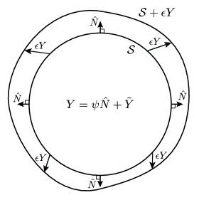
Figure 1.1. The MOTS stability operator $L_{\mathcal{S}}$ measures the change of the outward expansion $\theta_{+}$ if $\mathcal{S}$ is deformed in the $Y$ direction. In the figure $\tilde{Y}\in T\mathcal{S}$.

A schematic of a deformation is shown in Figure 1.1 and can be used to understand the stability classification of MOTS. $\mathcal{S}$ is said to be strictly stable or marginally stable respectively if there exists a not everywhere vanishing, non-negative $\psi$ such that $L_{\mathcal{S}}\psi>0$ or $L_{\mathcal{S}}\psi=0$. It is unstable if no such $\psi$ exists. It was shown in [2, 3] that this classification is equivalently determined by $\lambda_{1}>0$ (strictly stable), $\lambda_{1}=0$ (marginally stable) or $\lambda_{1}<0$ (unstable). Further, a strictly stable MOTS forms a boundary between trapped and untrapped regions in the sense that there is a two-sided neighbourhood $\mathcal{N}(\mathcal{S})$ that contains no complete outer trapped surfaces outside $\mathcal{S}$ and no complete outer untrapped surfaces inside. Thus, it can usefully be thought of as a generalization (and more computationally useful version) of an apparent horizon.

All exotic MOTS so far observed in either exact or numerical solutions have been found to be unstable. In this paper, we show why this must be true for a wide class of MOTS found in highly symmetric spacetimes.

1.2. Main results

We work in the $(n+1)$-formulation of general relativity. Initial data sets are then specified by $(\Sigma,g,K)$ where $\Sigma$ is an orientable $n$-dimensional manifold, $g$ is a Riemmanian metric and $K$ is a symmetric $(0,2)$-tensor on $\Sigma$ (the extrinsic curvature of $\Sigma$ in the full spacetime). In this setting, a MOTS is defined in the following way.

Definition 1.1.

Let $\mathcal{S}$ be a closed, orientable $(n-1)$-dimensional manifold that is smoothly immersed in $\Sigma$, with outward oriented unit normal $\hat{N}$ and induced metric $q$. The outward null expansion of $\mathcal{S}$ is

$$\theta_{+}=\Tr_{q}(K)+H=\Tr_{g}(K)-K(\hat{N},\hat{N})+H,$$ (1.2)

where $\Tr_{q}$ and $\Tr_{g}$ are the trace with respect to $q$ and $g$, respectively, while $H$ is the mean curvature of $\mathcal{S}$ in $\Sigma$. If $\theta_{+}=0$, then $\mathcal{S}$ is a marginally outer trapped surface (MOTS).

Remark 1.2.

There are a few points to note in this definition:

1. $\mathcal{S}$ is immersed, not necessarily embedded: self-intersections are allowed (and expected!).

2. Relative to the full spacetime, null normals to $\mathcal{S}$ can be written as

   $$\ell^{+}=\hat{u}+\hat{N}\qquad\qquad\ell^{-}=\hat{u}-\hat{N}$$ (1.3)

   where $\hat{u}$ is the future-pointing unit normal to $\Sigma$ in the full spacetime and $\hat{N}$ remains as the outward-pointing spacelike normal to $\mathcal{S}$ in $\Sigma$. Then the outward null expansion is equivalently

   $$\theta_{+}=\Tr_{q}(k_{+})$$ (1.4)

   where $k_{+}$ is the pull-back of the (spacetime) covariant derivative of $\ell_{+}$ to $\mathcal{S}$. In other words, $\theta_{+}$ is the mean curvature of $\mathcal{S}$ in the outward null direction. The choice of scaling for $\ell_{+}$ follows the convention of [2], which will facilitate the comparison with results from that paper.

3. The “O” in MOTS is a hold-over from a time when all known MOTS were embedded surfaces which had clear insides and outsides. Now, with the recognition that these surfaces can have much more complicated geometries, “outer” is often understood simply as a label which may or may not clearly correspond to an “outward” direction.

Next, we define a symmetry of an initial data set.

Definition 1.3.

A non-trivial vector field $X$ on $\Sigma$ is a symmetry of $(\Sigma,g,K)$ if $\mathcal{L}_{{}_{X}}g=\mathcal{L}_{{}_{X}}K=0$. It is a symmetry of a surface $\mathcal{S}$ if, in addition, it is everywhere tangent to $\mathcal{S}$.

It was observed in [3] that if $X$ is a symmetry of the initial data set and $\mathcal{S}$ is a strictly stable MOTS, then $X$ must also be a symmetry of $\mathcal{S}$. The converse is not true — knowing that $X$ is a symmetry of the initial data set and of $\mathcal{S}$ does not determine the stability of $\mathcal{S}$. For example, the outer and inner horizons of Reissner–Nördstrom black hole spacetimes share the spherical symmetry of the full spacetime but, away from extremality, the outer horizon is strictly stable while the inner horizon is unstable [10, 9]. In the extremal case, the horizons coincide and are marginally stable.

We are interested in the situation where $X$ is not a symmetry of $\mathcal{S}$. This means $\mathcal{S}$ is less symmetric than the initial data set containing it, since it is not invariant under the flow generated by $X$. In this case, $\mathcal{S}$ is either unstable or marginally stable. The following simple criterion allows us to distinguish between these cases.

Theorem 1.4.

Suppose $\mathcal{S}$ is a MOTS and $X$ is a symmetry of $(\Sigma,g,K)$ but not of $\mathcal{S}$.

1. $\mathcal{S}$ is marginally stable if and only if $X$ is nowhere tangent to $\mathcal{S}$.

2. $\mathcal{S}$ is unstable if and only if $X$ is tangent to $\mathcal{S}$ at some point.

The theorem implies, for instance, that any non-spherical MOTS in Schwarzschild is unstable. A large family of such MOTSs were found numerically in [8], and will be analyzed in Section 3.2 using the above theorem.

The marginally stable case will be discussed further in Section 4.6. For now, we just mention the example

$$\Sigma=\mathbb{R}\times\mathcal{S}_{0},\qquad g=dr^{2}+g_{0},$$ (1.5)

where $(\mathcal{S}_{0},g_{0})$ is a compact, orientable Riemannian manifold. Each hypersurface $\mathcal{S}=\{r\}\times\mathcal{S}_{0}$ is a minimal surface and hence a MOTS in the initial data set $(\Sigma,g,0)$. Moreover, $X=\frac{\partial}{\partial r}$ is a symmetry of the initial data set that is nowhere tangent to $\mathcal{S}$. Therefore, $\mathcal{S}$ is marginally stable.

Remark 1.5.

An important instance of Theorem 1.4 is when $\Sigma$ is a spacelike slice in a spacetime $(\mathcal{M},\bar{g})$, with $g$ and $K$ being the induced metric and second fundamental form. If $\bar{X}$ is a Killing vector field on $(\mathcal{M},\bar{g})$ that is tangent to $\Sigma$, then it is a symmetry of $(\Sigma,g,K)$; cf. [12, Cor. 1].

If $\mathcal{S}$ is the boundary of a compact region in $\Sigma$, we can give simple conditions under which the instability criteria in Theorem 1.4 are satisfied.

Theorem 1.6.

Suppose $\mathcal{S}$ is an embedded MOTS and $X$ is a symmetry of $(\Sigma,g,K)$. If $\mathcal{S}$ bounds a compact region $A\subset\Sigma$, then it is unstable under any of the following conditions:

1. $X$ is not a symmetry of $\mathcal{S}$;

2. $X$ is a coordinate vector field on $A$;

3. $\chi(\mathcal{S})\neq 0$ and $X$ has no zeros in $A$.

In particular, footnote 1 implies that for any initial data set with translational symmetry, all MOTS are unstable, therefore the boundary of the trapped region is not a MOTS (recalling that our definition requires a MOTS to be compact); see Section 3.3. In Section 3.4, we give an example where the trapped region is all of $\Sigma$ and thus the boundary is empty.

In three dimensions we get a stronger result.

Theorem 1.7.

Let $X$ be a symmetry of a three-dimensional initial data set $(\Sigma,g,K)$. If $\mathcal{S}$ is a stable MOTS that bounds a compact region in $\Sigma$ and has $\chi(\mathcal{S})\neq 0$, then it must intersect the zero set of $X$.

For instance, if $(\Sigma,g,K)$ satisfies the dominant energy condition, any strictly stable MOTS (which necessarily has spherical topology) must intersect the zero set of $X$. The same is true of the apparent horizon, provided it is a compact surface. See Section 3.3 for further discussion.

Another easy consequence of Theorem 1.4 is that in three spatial dimensions, a MOTS of genus greater than one cannot be strictly stable when $(\Sigma,g,K)$ has a symmetry.

Corollary 1.8.

Suppose $\mathcal{S}$ is a MOTS and $X$ is a symmetry of $(\Sigma,g,K)$. If $\dim\Sigma=3$ and $\mathcal{S}$ is a surface of genus $\mathfrak{g}\geq 2$, then it is either unstable or marginally stable.

Remark 1.9.

Unlike Theorem 1.6, this result does not assume that $X$ is nowhere vanishing or that $\mathcal{S}$ bounds a region in $\Sigma$. It is not possible to rule out the marginally stable case under these weaker hypotheses, as demonstrated by the example in (1.5). On the other hand, if the dominant energy condition holds, a MOTS of positive genus cannot be strictly stable, and a MOTS of genus $\mathfrak{g}\geq 2$ must be unstable [17]. While the existence of a symmetry is a strong assumption on the initial data set, it is interesting to note that no energy conditions are needed in 1.8.

In the proof of Theorem 1.4, we will see that $0$ is an eigenvalue of $L_{\mathcal{S}}$ with associated eigenfunction $\psi=g(X,\hat{N})$, where $\hat{N}$ is a unit normal vector field along $\mathcal{S}$. When $L_{\mathcal{S}}$ is self-adjoint, or at least is similar to a self-adjoint operator, we can obtain additional information about its spectrum from the structure of $\psi$. In Lemma 2.1, we give a sufficient condition for $L_{\mathcal{S}}$ to be similar to a self-adjoint operator, in terms of the so-called Hájiček one-form $\omega$, defined in (2.3).

Defining the nodal domains of $\psi$ to be the connected components of $\{p\in\mathcal{S}:\psi(p)\neq 0\}$, and letting $\nu(\psi)$ denote the number of nodal domains, we then have the following consequence of Courant’s nodal domain theorem.

Theorem 1.10.

If the hypotheses of Theorem 1.4 are satisfied and the Hájiček one-form $\omega$ is exact, then $L_{\mathcal{S}}$ has at least $\nu(\psi)-1$ negative eigenvalues.

In Section 3.2, we will use this to obtain a lower bound on the number of unstable eigenvalues for the self-intersecting MOTS in Schwarzschild that were recently observed in [8].

Outline of the paper

In Section 2, we review the definition of the stability operator. In Section 3, we give applications to initial data sets with rotational or translation symmetry. The proofs of the main theorems are postponed until Section 4.

2. The MOTS stability operator

As noted in the introduction, the stability operator measures the variation of $\theta_{+}$ when $\mathcal{S}$ is deformed along the flow generated by a vector field $Y\in T\Sigma$. Decomposing $Y$ on $\mathcal{S}$ into normal and tangential parts, $Y=\psi\hat{N}+\tilde{Y}$, it is straightforward to see that this variation depends only on the normal component:

$$\delta_{Y}\theta_{+}=\delta_{\psi\hat{N}}\theta_{+}+\delta_{\tilde{Y}}\theta_{+}=\delta_{\psi\hat{N}}\theta_{+}\;.$$ (2.1)

The $\delta_{\tilde{Y}}\theta_{+}$ part of the deformation amounts to a shift over $\mathcal{S}$ and so vanishes for a MOTS.

The variation only depends on the values of $\psi$ on $\mathcal{S}$ and is given by the action of an elliptic operator on $\psi$. This is a more involved calculation but one that has appeared in many different versions over the last few decades (see, for example, [28, 3]). If $\mathcal{S}$ is a MOTS, then the result is

$$\delta_{Y}\theta_{+}=L_{\mathcal{S}}\psi$$

for $\psi=g(Y,\hat{N})$ and

$${L}_{\mathcal{S}}{\psi}=\left[-(\mathcal{D}^{A}-{\omega}^{A})(\mathcal{D}_{A}-{\omega}_{A})+\tfrac{1}{2}\left(R^{(2)}-\|\sigma_{+}\|^{2}-{G}_{++}-{G}_{+-}\right)\right]{\psi}\;.$$ (2.2)

In this equation, $\mathcal{D}_{A}$ is the Levi-Civita connection associated with the induced two-metric $q_{AB}$,

$${\omega}_{A}=e_{A}^{a}K_{ab}\hat{N}^{b}=-\tfrac{1}{2}e_{A}^{\alpha}{\ell}^{-}_{\beta}\nabla_{\alpha}{\ell}_{+}^{\beta}$$ (2.3)

is the connection on the normal bundle (also known as the Hájiček one-form, which is associated with angular momentum [16]), $R^{(2)}$ is the Ricci scalar of the two-metric $q_{AB}$, $\sigma_{+}=k_{+}-\frac{1}{2}\Tr(k_{+})q$ is the shear of $\ell_{+}$ on $\mathcal{S}$ and

$$G_{++}={G}({\ell}^{+},{\ell}^{+})\mbox{ and }G_{+-}={G}({\ell}^{+},{\ell}^{-})$$ (2.4)

are components of the Einstein tensor ${G}$ of $\bar{g}$ over $\mathcal{M}$. $L_{\mathcal{S}}$ takes a slightly different form if the null vectors are scaled differently than in (1.3); however, such changes leave the eigenvalues unchanged.

If $\omega=0$, then $L_{\mathcal{S}}$ is self-adjoint, in which case all eigenvalues are real. If $\omega\neq 0$ then this is not the case in general. For instance, the stability operator for the Kerr black hole has complex eigenvalues provided the angular momentum is nonzero [11]. There is, however, a special case in which $L_{\mathcal{S}}$ is similar to a self-adjoint operator and hence has real eigenvalues.

Lemma 2.1.

Given the operator $L_{\mathcal{S}}$ defined by (2.2), if $\omega=\mathcal{D}f$ for some function $f$, then $L_{\mathcal{S}}$ is similar to the self-adjoint operator

$${\tilde{L}}_{\mathcal{S}}=-\mathcal{D}^{A}\mathcal{D}_{A}+\tfrac{1}{2}\left(R^{(2)}-\|\sigma_{+}\|^{2}-{G}_{++}-{G}_{+-}\right)$$ (2.5)

in the sense that $L_{\mathcal{S}}\psi=e^{f}\tilde{L}_{\mathcal{S}}(e^{-f}\psi)$ for all $\psi$. In particular, $L_{\mathcal{S}}$ and $\tilde{L}_{\mathcal{S}}$ have the same eigenvalues, and their eigenfunctions are related by $\psi=e^{f}\tilde{\psi}$.

For deformations in the null direction $\ell_{-}$, this was shown in [22, 23]. For the spacelike deformations considered here, the proof is essentially the same, but for completeness, we present it below.

Proof of Lemma 2.1.

If $\omega=\mathcal{D}f$ and $T$ is any tensor field, then

$$(\mathcal{D}-\omega)(e^{f}T)=e^{f}(T\mathcal{D}f+\mathcal{D}T-\omega T)=e^{f}\mathcal{D}T\;,$$ (2.6)

and so $L_{\mathcal{S}}(e^{f}\tilde{\psi})=e^{f}\tilde{L}_{\mathcal{S}}\tilde{\psi}$. ∎

The stability operator plays a key role in understanding the evolution of MOTS for dynamical black holes. In [2, 3] it was shown that a strictly stable MOTS can be locally evolved into the past and future as a marginally outer trapped tube (MOTT). The same is true of any MOTS for which $L_{\mathcal{S}}$ has no vanishing eigenvalues, with strictly stable MOTS being a special case (since $\lambda_{1}>0$ implies all eigenvalues have positive real part and hence are nonzero).

If $L_{\mathcal{S}}$ has a vanishing eigenvalue, then evolution into the past or future is not guaranteed. However, this is not a surprise. Going back as far as [18], it has been recognized that apparent horizons can “jump” and, when they do, they immediately split into a pair of MOTSs, one expanding in area and the other shrinking. These are the “pair creations” mentioned in the introduction. Pairs can also annihilate. These behaviours have been seen in binary mergers (for example [34, 33, 13, 15, 31]) and in exact solutions (for example [6, 5, 21]). In all observed cases, the MOTS that appears (disappears) in a creation (annihilation) event has a vanishing eigenvalue of $L_{\mathcal{S}}$ (but not necessarily $\lambda_{1}$). Returning to the deformation interpretation of that stability operator, as given by (1.1), these are cases where the marginally outer trapped tube containing the MOTS becomes tangent to $\Sigma$.

An important result in this direction is [1, Prop 5.1], which says that, under a suitable genericity assumption, every marginally stable MOTS is contained in a smooth MOTT that is tangent to $\Sigma$. The case where $\lambda_{1}<0$ but a higher eigenvalue of $L_{\mathcal{S}}$ vanishes is more delicate and, to the best of our knowledge, has not yet been studied analytically.

3. Applications

3.1. Spherical symmetry

We first prove a general result for initial data sets with spherical symmetry.

Theorem 3.1.

If $\Sigma\subset\mathbb{R}^{3}$ and $(\Sigma,g,K)$ is a spherically symmetric initial data set, then any non-spherical MOTS $\mathcal{S}$ in $\Sigma$ is unstable.

Note that we do not require $\Sigma$ to be all of $\mathbb{R}^{3}$, so we could have $\Sigma=\mathbb{R}^{3}\backslash\{0\}$, for instance. In particular, we conclude that any non-spherical MOTS in Schwarzschild must be unstable. This demonstrates that all of the exotic MOTS found in [8, 20] are unstable. We will recall these solutions and investigate their instability further in Section 3.2.

Remark 3.2.

If $\mathcal{S}$ is a sphere, then Theorem 1.4 does not apply and anything is possible. For instance, there are spherical MOTS in Reissner–Nordström that are strictly stable, marginally stable and unstable for appropriate choices of mass and charge [10, 20, 9].

Proof of Theorem 3.1.

Consider the vector fields $R_{x}$, $R_{y}$ and $R_{z}$ that generate rotations about the $x$, $y$ and $z$ axes, respectively. Since $\mathcal{S}$ is not spherically symmetric, there exists a linear combination of these, which we call $X$, that is not everywhere tangent to $\mathcal{S}$. Let us prove that $X$, which is a symmetry of $(\Sigma,g,K)$, is somewhere tangent to $\mathcal{S}$.

Consider the restriction $f:=r\big{|}_{\mathcal{S}}$ of the radial coordinate to $\mathcal{S}$. Since $\mathcal{S}$ is compact, $f$ has a maximum at some point $p\in\mathcal{S}$, thus $\nabla^{\mathcal{S}}f(p)=0$. Decomposing the gradient of $r$ into normal and tangential components along $\mathcal{S}$,

$$\nabla r=\nabla^{\mathcal{S}}f+(\nabla_{\hat{N}}r)\hat{N},$$

shows that $\hat{N}_{p}$ is proportional to $\nabla r(p)$. Since $R_{x}$, $R_{y}$, and $R_{z}$ are orthogonal to $\nabla r(p)$, they are also orthogonal to $\hat{N}_{p}$ and hence are contained in $T_{p}S$. This means $X_{p}\in T_{p}\mathcal{S}$, so we can apply Theorem 1.4 to conclude that $\mathcal{S}$ is unstable. ∎

If we assume that $\mathcal{S}$ is axisymmetric and the one-form $\omega$ is exact, we get a stronger result. Letting $(r,\theta,\phi)$ denote the standard spherical coordinates for $\mathbb{R}^{3}$, an axisymmetric surface can be parameterized as

$$(r,\theta,\phi)=\big{(}P(s),\Theta(s),\phi\big{)}$$ (3.1)

for some functions $P$ and $\Theta$.

Theorem 3.3.

Suppose $\mathcal{S}$ is an axisymmetric MOTS parameterized by $\big{(}P(s),\Theta(s)\big{)}_{s\in[a,b]}$. If $\omega$ is exact and $P$ is not constant, then $L_{\mathcal{S}}$ has at least $2C(P)+1$ negative eigenvalues, where $C(P)$ is the number of critical points of $P$ in $(a,b)$.

Remark 3.4.

It is implicit in the conclusion of the theorem that $C(P)$ is finite whenever $P$ is not constant. Of course, this is not true for an arbitrary smooth function, but $P$ here is highly constrained, since $\big{(}P(s),\Theta(s)\big{)}$ parameterizes a MOTS.

Proof.

The tangent space to $\mathcal{S}$ at a point $p=\big{(}P(s),\Theta(s),\phi\big{)}$ is spanned by

$$\left\{P^{\prime}(s)\frac{\partial}{\partial r}+\Theta^{\prime}(s)\frac{\partial}{\partial\theta},\ \frac{\partial}{\partial\phi}\right\}.$$

Writing $g=dr^{2}+A(r)^{2}d\Omega^{2}$, we calculate the outward unit normal

$$\hat{N}_{p}=a(s)\left[A\big{(}P(s)\big{)}^{2}\Theta^{\prime}(s)\frac{\partial}{\partial r}-P^{\prime}(s)\frac{\partial}{\partial\theta}\right],$$ (3.2)

where $a(s)>0$ is a normalization constant. Using the change of coordinates

$$\begin{array}[]{l}x=r\sin\theta\cos\phi\\ y=r\sin\theta\sin\phi\\ z=r\cos\theta\end{array}\qquad\longrightarrow\qquad\begin{array}[]{l}\displaystyle\frac{\partial}{\partial x}=\sin\theta\cos\phi\frac{\partial}{\partial r}+\frac{\cos\phi\cos\theta}{r}\frac{\partial}{\partial\theta}-\frac{\sin\phi}{r\sin\theta}\frac{\partial}{\partial\phi}\\[8.61108pt] \displaystyle\frac{\partial}{\partial z}=\cos\theta\frac{\partial}{\partial r}-\frac{\sin\theta}{r}\frac{\partial}{\partial\theta}\end{array}$$

the rotation in the $x$-$z$ plane can be rewritten as

$$X:=z\frac{\partial}{\partial x}-x\frac{\partial}{\partial z}=\cos\phi\frac{\partial}{\partial\theta}-\sin\theta\cot\phi\frac{\partial}{\partial\phi}\,.$$ (3.3)

Using this and (3.2), we compute

$$\psi=g(X,\hat{N})=g\left(\cos\phi\frac{\partial}{\partial\theta},-P^{\prime}(s)\frac{\partial}{\partial\theta}\right)=-a(s)A\big{(}P(s)\big{)}^{2}P^{\prime}(s)\cos\phi.$$ (3.4)

As expected, we see that $\psi$ is not identically zero as long as $P(s)$ is not constant, i.e., the surface it parameterizes is not a sphere. In this case, $\psi$ is an eigenfunction of $L_{\mathcal{S}}$. Up to a non-vanishing factor, it is proportional to $P^{\prime}(s)\cos\phi$.

Since $\cos\phi$ changes sign on $\mathcal{S}$ (recall that $0<\phi<2\pi$), we conclude that $\psi$ has twice as many nodal domains as $P^{\prime}(s)$. Letting $C(P)$ denote the number of critical points of $P$, we thus have $\nu(\psi)=2\big{(}C(P)+1\big{)}=2C(P)+2$, and so by Theorem 1.10, $L_{\mathcal{S}}$ has at least $2C(P)+1$ negative eigenvalues. ∎

Remark 3.5.

In the proof we also could have chosen the symmetry $X$ to be rotation in the $y$-$z$ plane. This gives a second linearly independent function in $\ker L_{\mathcal{S}}$, namely $P^{\prime}(s)\sin\phi$.

3.2. Exotic MOTS in Schwarzschild

We now consider a concrete application of Theorem 3.3. For that we focus on the exotic MOTS in the Schwarzschild spactime, which originally appeared in [8].

For Painlevé–Gullstrand slices of Schwarzschild we have

$$g =\differential r\otimes\differential r+r^{2}\left(\differential\theta\otimes\differential\theta+\sin^{2}\!\theta\,\differential\phi\otimes\differential\phi\right)$$ (3.5)

$$K =\sqrt{\frac{m}{2r^{3}}}\differential r\otimes\differential r-\sqrt{2mr}\left(\differential\theta\otimes\differential\theta+\sin^{2}\!\theta\,\differential\phi\otimes\differential\phi\right)$$ (3.6)

in spherical coordinates $(r,\theta,\phi)$. Parameterizing axisymmetric surfaces in $\Sigma$ by $\big{(}P(s),\Theta(s)\big{)}$ as in (3.1), and letting $s$ be the arc-length along curves of constant $\phi$ as measured from the “north pole,” the equation $\theta_{+}=0$ becomes a pair of second-order differential equations for $P$ and $\Theta$; see [9]. We do not need their exact form here but show some solutions to the equations in Figure 3.1. These so-called “MOTSodesics” are rotated into MOTS by the action of $\partialderivative{\phi}$.

The exact form of the stability operator is also not important here, we just need to know if it is similar to a self-adjoint operator. To that end, one can calculate the Hájiček one-form

$$\omega=3\sqrt{\frac{m}{2P}}\dot{P}\dot{\Theta}\,\differential s\,.$$ (3.7)

This is closed and hence exact, since $H^{1}(S^{2};\mathbb{R})$ is trival. We can thus use Theorem 3.3 to bound the number of negative eigenvalues for $L_{\mathcal{S}}$.

From the parameterized curves given in Figure 3.1 (a version of which originally appeared in [8]), we observe that $C(P)=1,3,5,7,9$, going from left to right, therefore $L_{\mathcal{S}}$ has at least $3,7,11,15,19$ negative eigenvalues for these solutions. More generally, a solution with $n$ loops has $2n-1$ critical points ($n$ minima and $n-1$ maxima), so there are at least $2(2n-1)+1=4n-1$ negative eigenvalues.

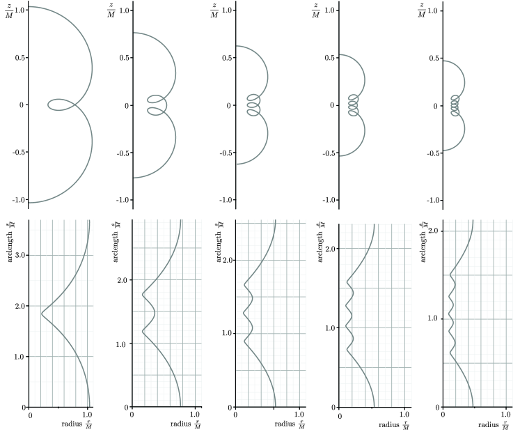
Figure 3.1. Top: solution curves $(r,\theta)=\big{(}P(s),\Theta(s)\big{)}$ to the “MOTSodesic equations” in the $\phi=0$ plane. Bottom: the radial function $P(s)$.

3.3. Spatial translations and the apparent horizon

An immediate consequence of Theorem 1.6 is that if $(\Sigma,g,K)$ admits a symmetry given by a (global) coordinate vector field, then every MOTS that bounds a compact region is unstable. Similarly, if $(\Sigma,g,K)$ admits a non-vanishing symmetry, then any MOTS with $\chi(\mathcal{S})\neq 0$ is unstable.

We now apply these results to the apparent horizon. Recalling that a surface is weakly outer trapped if $\theta_{+}\leq 0$, we define the outer trapped region, $\mathcal{T}$, to be the union of all regions in $\Sigma$ with weakly outer trapped boundary. The apparent horizon is then defined to be the boundary of the outer trapped region. It is well known that if $\partial\mathcal{T}$ is smooth, then it must have $\theta_{+}=0$. If, in addition, it is compact, then it is a stable MOTS, so Theorem 1.6 implies the following.

Corollary 3.6.

Suppose $X$ is a symmetry of $(\Sigma,g,K)$. If $X$ is a coordinate vector field, then $\partial\mathcal{T}$ is not a compact hypersurface.

In other words, one of the following must occur: 1) $\partial\mathcal{T}$ is empty; 2) $\partial\mathcal{T}$ is not smooth; 3) $\partial\mathcal{T}$ is a smooth, non-compact hypersurface with $\theta_{+}=0$.

The smoothness of the apparent horizon is a delicate issue. If $\partial\mathcal{T}$ is piecewise smooth, then it is in fact smooth and has $\theta_{+}=0$, by [26, Prop. 7]. On the other hand, in [4, Thm. 7.3] it was shown that $\partial\mathcal{T}$ is smooth if the initial data set is compact and has outer untrapped boundary. (For instance, if $(\Sigma,g,K)$ is asymptotically flat, this can be applied to a large coordinate sphere in the asymptotic region.) While this latter theorem has no a priori regularity requirements on $\partial\mathcal{T}$, the required boundary behaviour rules out initial data sets with translational symmetry.

A similar result to 3.6 holds if we assume that $X$ is nowhere vanishing and $\chi(\partial\mathcal{T})\neq 0$. Furthermore, this topological restriction can be eliminated in three-dimensional initial data sets satsfying the dominant energy condition (DEC), since in that case the apparent horizon must have spherical topology (assuming it is smooth and compact).

Corollary 3.7.

Let $X$ be a symmetry of a three-dimensional initial data set $(\Sigma,g,K)$ that satisfies the dominant energy condition. If $\partial\mathcal{T}$ is a compact hypersurface, then it must intersect the zero set of $X$.

In particular, this implies that if $X$ is nowhere vanishing, then $\partial\mathcal{T}$ is not a compact hypersurface. On the other hand, when the apparent horizon is a compact hypersurface, this gives us some clue as to where it is located.

3.4. MOTS in FLRW

Consider a flat FLRW cosmology. This has metric [18]

$$\differential s^{2}=-\differential t^{2}+a(t)^{2}\left(\differential x^{2}+\differential y^{2}+\differential z^{2}\right)$$ (3.8)

for scale factor $a(t)$. We are interested in a $(3+1)$-formulation and so foliate with three-surfaces $(\Sigma_{t},g_{t},K_{t})$ of constant $t$. These surfaces have induced metric

$$g_{t}=a(t)^{2}(\differential x^{2}+\differential y^{2}+\differential z^{2})$$ (3.9)

and extrinsic curvature

$$K_{t}=\left(\frac{\dot{a}(t)}{a(t)}\right)g_{t},$$ (3.10)

with the dot indicating a derivative with respect to $t$. For the rest of the section, we will suppress the $t$ dependence in $a$ and $\dot{a}$.

For any $t$, (3.9) is simply a constant scaling of the Euclidean metric and so it has the same Killing fields, namely the translations $\big{\{}\partialderivative{x},\partialderivative{y},\partialderivative{z}\big{\}}$ and the rotations. The extrinsic curvature is proportional to the metric (3.9), so each of these Killing fields is a symmetry of $(\Sigma_{t},g_{t},K_{t})$.

It follows immediately from Theorem 1.6 that every MOTS in $(\Sigma_{t},g_{t},K_{t})$ is unstable; thus, the boundary of the trapped region cannot be a MOTS. We now demonstrate this explicitly by showing that the trapped region is, in fact, all of $\Sigma$; therefore, its boundary is empty.

Since $\Sigma_{t}=\mathbb{R}^{3}$, we denote points in space by $\mathbf{x}=(x,y,z)$, so the two-sphere of coordinate radius $r_{o}$, centred at $\mathbf{x}_{o}=(x_{o},y_{o},z_{o})$, is given by

$$(x-x_{o})^{2}+(y-y_{o})^{2}+(z-z_{o})^{2}=r_{o}^{2}\;.$$ (3.11)

The mean curvature of such a coordinate sphere with respect to $g_{t}$ is $H=2/ar_{o}$ and so, using (3.10), the outward null expansion is

$${\theta}_{+} =\frac{2(1+\dot{a}r_{o})}{ar_{o}}\;.$$ (3.12)

If $\dot{a}<0$ at the time in question, it follows that any coordinate sphere of radius $r_{o}=-1/\dot{a}$ is a MOTS in $(\Sigma_{t},g_{t},K_{t})$, and any coordinate sphere of radius $r_{o}<-1/\dot{a}$ is an outer trapped surface. This justifies the claim made above that the trapped region is all of $\Sigma$.

The action of the translational Killing vector fields on the coordinate spheres is simply to move the centre point $\mathbf{x}_{o}$. From the proof of Theorem 1.4, in particular Lemma 4.1, we know that each translational vector field $X$ generates a non-trivial function $\psi=g(X,\hat{N})$ in the kernel of $L_{\mathcal{S}}$. In fact, each of the translations $\big{\{}\partialderivative{x},\partialderivative{y},\partialderivative{z}\big{\}}$ generates a linearly independent function, which we now calculate. Taking $\mathbf{x}_{o}=(0,0,0)$ for simplicity, the unit normal to $\mathcal{S}$ is

$$\hat{N}=\frac{1}{ar_{o}}\mathbf{x},$$ (3.13)

and so at any point $\mathbf{x}=(r_{o}\sin\theta\cos\phi,r_{o}\sin\theta\sin\phi,r_{o}\cos\theta)$ on $\mathcal{S}$ we have

$$g\left(\partialderivative{x},\hat{N}\right) =\frac{a}{r_{o}}x=a\sin\theta\cos\phi,$$

$$g\left(\partialderivative{y},\hat{N}\right) =\frac{a}{r_{o}}y=a\sin\theta\sin\phi,$$ (3.14)

$$g\left(\partialderivative{z},\hat{N}\right) =\frac{a}{r_{o}}z=a\cos\theta,$$

which are linear combinations of the $l=1$ spherical harmonics.

In this case, $L_{\mathcal{S}}$ can also be computed directly. Calculating the terms of (2.2), the Ricci scalar of the coordinate sphere is $R^{(2)}=2/(ar_{o})^{2}$, while by direct calculation the Einstein terms are $G_{++}=-2(a\ddot{a}-\dot{a}^{2})/a^{2}$ and $G_{+-}=2(a\ddot{a}+\dot{a}^{2})/a^{2}$, whence

$$\frac{1}{2}\left(G_{++}+G_{+-}\right)=\frac{2\dot{a}^{2}}{a^{2}}=\frac{2}{a^{2}r_{o}^{2}}$$ (3.15)

with the second equality following from (3.12). Since $\omega=0$, the stability operator takes the form

$$L_{\mathcal{S}}\psi=-\frac{1}{r_{o}^{2}}\left(\Delta\psi+2\psi\right)$$ (3.16)

where $\Delta$ is the Laplacian on the unit sphere. For each $l=0,1,2,\ldots$ we have that $\big{(}l(l+1)-2\big{)}/r_{o}^{2}$ is an eigenvalue of multiplicity $2l+1$, with eigenspace spanned by the spherical harmonics $Y_{l}^{m}(\theta,\phi)$ for $|m|\leq l$. In particular, $L_{\mathcal{S}}$ has one negative eigenvalue, with $l=0$, and a three-dimensional kernel spanned by the $l=1$ spherical harmonics, as seen above.

The advantage of Theorem 1.4 is that it allows us to determine these eigenfunctions directly from symmetry principles, without even writing down an explicit formula for $L_{\mathcal{S}}$.

4. Proofs

We now prove our main theorems and discuss the marginally stable case in more detail.

4.1. Proof of Theorem 1.4

Throughout this subsection, we assume the hypotheses of the theorem, namely that $\mathcal{S}$ is a MOTS in $(\Sigma,g,K)$ and $X$ is a symmetry of $(\Sigma,g,K)$ but not a symmetry of $\mathcal{S}$.

Lemma 4.1.

$0$ is an eigenvalue of $L_{\mathcal{S}}$, with eigenfunction $\psi=g(X,\hat{N})$.

Proof.

We first observe that for any diffeomorphism $\varphi$ of $\Sigma$, the surface $\varphi(\mathcal{S})$ is a MOTS in the initial data set $\big{(}\Sigma,(\varphi^{-1})^{*}g,(\varphi^{-1})^{*}K\big{)}$. Now let $\varphi_{t}$ denote the flow generated by $X$. The symmetry conditions $\mathcal{L}_{{}_{X}}g=\mathcal{L}_{{}_{X}}K=0$ guarantee that $g$ and $K$ are invariant under this flow, meaning that for all $t$ we have $(\varphi_{t}^{-1})^{*}g=(\varphi_{-t})^{*}g=g$, and analogously for $K$. It follows that $\mathcal{S}_{t}=\varphi_{t}(\mathcal{S})$ is a MOTS in the initial data set $(\Sigma,g,K)$, therefore

$$0=\delta_{X}\theta_{+}=L_{\mathcal{S}}\psi,$$ (4.1)

with $\psi=g(X,\hat{N})$. Since $X$ is not everywhere tangent to $\mathcal{S}$, the function $\psi$ is not identically zero, and hence is an eigenfunction of $L_{\mathcal{S}}$ with $0$ eigenvalue. ∎

The next lemma characterizes when $0$ is the principal eigenvalue of $L_{\mathcal{S}}$.

Lemma 4.2.

The principal eigenvalue of $L_{\mathcal{S}}$ is $0$ if and only if $\psi$ is sign definite.

Here sign definite is meant in the strict sense, i.e., everywhere positive or everywhere negative.

Proof.

If $\psi$ is the principal eigenfunction, then it must be sign definite by [2, Lem. 1]. If $\psi$ is not the principal eigenfunction, then the principal eigenvalue $\lambda_{1}$ is negative (and in particular nonzero). This is also the principal eigenvalue of the adjoint $L_{\mathcal{S}}^{*}$, and the corresponding eigenfunction $\phi$ is sign definite (again by [2]). We then compute

$$\lambda_{1}\int_{\mathcal{S}}\phi\psi=\int_{\mathcal{S}}(L^{*}_{\mathcal{S}}\phi)\psi=\int_{\mathcal{S}}\phi L_{\mathcal{S}}\psi=0$$

and conclude that $\psi$ changes sign. ∎

Observing that $\psi=g(X,\hat{N})$ is sign definite if and only if $X$ is nowhere tangent to $\mathcal{S}$ completes the proof of Theorem 1.4.

4.2. Proof of Theorem 1.6

Item 1 is an immediate consequence of Theorem 1.4 and the following.

Lemma 4.3.

If $\mathcal{S}$ is the boundary of a compact region $A\subset\Sigma$ and $X$ is a Killing vector field on $A$, then $X$ is tangent to $\mathcal{S}$ at some point.

Proof.

$X$ being a Killing vector field implies that $\operatorname{div}X=0$, and by the divergence theorem

$$0=\int_{A}\operatorname{div}X=\int_{\mathcal{S}}g(X,\hat{N}),$$

thus $g(X,\hat{N})$ has to vanish somewhere on $\mathcal{S}$. ∎

We next prove footnote 1. We know from Lemma 4.3 that $X$ is tangent to $\mathcal{S}$ somewhere, so we just need to show that it is not everywhere tangent to $\mathcal{S}$.

Lemma 4.4.

Suppose $\mathcal{S}$ is the boundary of a compact region $A\subset\Sigma$ and $X$ is a Killing vector field on $A$. If $X=\frac{\partial}{\partial x^{n}}$ for some coordinates $(x^{1},\ldots,x^{n})$ defined on an open set $U$ containing $A$, then $X$ is not everywhere tangent to $\mathcal{S}$.

Proof.

Since $\operatorname{div}X=0$, the vector field $Y:=x^{n}X$ has $\operatorname{div}Y=g\big{(}\nabla x^{n},\frac{\partial}{\partial x^{n}}\big{)}=1$. The divergence theorem then gives

$$\int_{\mathcal{S}}x^{n}g(X,\hat{N})=\int_{\mathcal{S}}g(Y,\hat{N})=\int_{A}\operatorname{div}Y\neq 0,$$

which implies $g(X,\hat{N})$ is not identically zero on $\mathcal{S}$. ∎

Item 3 of Theorem 1.6 is a consequence of the following.

Lemma 4.5.

Suppose $\mathcal{S}$ is the boundary of a compact region $A\subset\Sigma$. If $\chi(\mathcal{S})\neq 0$ and $X$ has no zeros in $A$, then $X$ is tangent to $\mathcal{S}$ somewhere but not everywhere.

Proof.

If $g(X,\hat{N})\geq 0$ on all of $\mathcal{S}$, we can use the Poincaré–Hopf theorem to obtain $\chi(A)=0$, since $X$ has no zeros. On the other hand, if $\chi(\mathcal{S})\neq 0$ then $\mathcal{S}$ must be even dimensional, in which case $\chi(A)=\frac{1}{2}\chi(S)\neq 0$. This contradiction implies $g(X,\hat{N})(p)<0$ at some point $p\in S$. Applying the same argument to $-X$, we find a point $p^{\prime}\in\mathcal{S}$ with $g(X,\hat{N})(p^{\prime})>0$. It follows that $g(X,\hat{N})$ equals zero somewhere but not everywhere. ∎

4.3. Proof of Theorem 1.7

Note that Lemma 4.5 does not use the fact that $X$ is Killing. In three dimensions we can use this information to obtain the following refinement, which implies Theorem 1.7.

Lemma 4.6.

Suppose $\dim\Sigma=3$ and $\mathcal{S}$ is the boundary of a compact region $A\subset\Sigma$. If $\chi(\mathcal{S})\neq 0$ and $X$ is a Killing field with no zeros on $\mathcal{S}$, then $X$ is tangent to $\mathcal{S}$ somewhere but not everywhere.

Proof.

Consider the set $\mathcal{Z}=\{p\in A:X_{p}=0\}$. By assumption this does not intersect $\mathcal{S}$. From [25] we have $\mathcal{Z}=\cup V_{i}$, where each $V_{i}$ is a totally geodesic submanifold of even codimension. Since $n=3$, this means each $V_{i}$ is the image of a geodesic. Moreover, each $V_{i}$ is closed and hence compact, so it must be diffeomorphic to the circle.

It is therefore possible to perturb $X$ in the interior of $A$ (more precisely, in a tubular neighbourhood of each $V_{i}$) to obtain a vector field with no zeros, so the Poincaré–Hopf theorem implies $\chi(A)=0$. This is a contradiction because $\chi(\mathcal{S})\neq 0$ implies $\chi(A)\neq 0$. As in the proof of Lemma 4.5, we conclude that $g(X,\hat{N})$ changes sign on $\mathcal{S}$. ∎

4.4. Proof of 1.8

Assuming $\mathcal{S}$ has genus $\mathfrak{g}\geq 2$, it suffices to prove that $X$ is not a symmetry of $\mathcal{S}$. If it was, it would be everywhere tangent to $\mathcal{S}$ and hence would be a Killing vector field for the induced metric $q$ on $\mathcal{S}$. However, it is well known that a surface of genus $\mathfrak{g}\geq 2$ admits no non-trivial Killing fields. (In two dimensions the zeros of a non-trivial Killing vector field are isolated with index $+1$, so the Poincaré–Hopf theorem gives $\chi(\mathcal{S})\geq 0$ and hence $\mathfrak{g}\leq 1$.)

4.5. Proof of Theorem 1.10

Assuming the hypotheses of the theorem, namely $\omega=\mathcal{D}f$ for some function $f$, Lemma 2.1 guarantees that $L_{\mathcal{S}}$ has only real eigenvalues. We write these as $\lambda_{1}<\lambda_{2}\leq\lambda_{3}\leq\cdots$, repeated according to their multiplicity.

Lemma 4.7.

Assume the hypotheses of Theorem 1.10. If $\lambda$ is an eigenvalue of $L_{\mathcal{S}}$, then any eigenfunction for $\lambda$ has at most $\min\{k:\lambda_{k}=\lambda\}$ nodal domains.

Proof.

For the self-adjoint operator $\tilde{L}_{\mathcal{S}}$ defined in (2.5) this is precisely the statement of Courant’s nodal domain theorem. The same is true for $L_{\mathcal{S}}$, since it has the same eigenvalues as $\tilde{L}_{\mathcal{S}}$, and the corresponding eigenfunctions $\psi$ and $\tilde{\psi}=e^{f}\psi$ have the same nodal domains. ∎

Remark 4.8.

The quantity $\min\{k:\lambda_{k}=\lambda\}$ is called the “spectral position” or “minimal label” of $\lambda$. For instance, if $\lambda_{1}<\lambda_{2}=\lambda_{3}=\lambda_{4}$ (as for the eigenvalues of the spherical Laplacian), the common eigenvalue $\lambda_{2}=\lambda_{3}=\lambda_{4}$ has minimal label $k=2$.

From the proof of Theorem 1.4, we know that 0 is an eigenvalue of $L_{\mathcal{S}}$. Observing that $L_{\mathcal{S}}$ has precisely $\min\{k:\lambda_{k}=0\}-1$ negative eigenvalues completes the proof of Theorem 1.10.

4.6. The marginally stable case

We now show that the marginally stable case of Theorem 1.4, in which the vector field $X$ is nowhere tangent (i.e., transversal) to $\mathcal{S}$ can only occur in certain geometries.

Theorem 4.9.

If $\mathcal{S}$ is a MOTS in $(\Sigma,g,K)$ and $X$ is a Killing vector field transversal to $\mathcal{S}$, then $\Tr_{q}(K)$ either vanishes identically (in which case $\mathcal{S}$ is a minimal surface) or changes sign on $\mathcal{S}$.

For instance, if $K$ is sign definite, as in the FLRW example of Section 3.4, the marginally stable case is prohibited.

Proof.

Letting $S\overset{\jmath}{\hookrightarrow}\Sigma$ denote the inclusion of $\mathcal{S}$ into $\Sigma$, we have

$$\mathcal{L}_{\tilde{X}}q=\mathcal{L}_{\tilde{X}}(\jmath^{*}g)=\jmath^{*}(\mathcal{L}_{\jmath_{*}\tilde{X}}g)=\jmath^{*}(\mathcal{L}_{X-\psi\hat{N}}g)=\jmath^{*}(\mathcal{L}_{X}g-\mathcal{L}_{\psi\hat{N}}g)=\jmath^{*}(0-\psi\mathcal{L}_{\hat{N}}g)=-2\psi k,$$

where $k$ is the extrinsic curvature of $\mathcal{S}$ in $\Sigma$. Taking the $q$-trace and using the fact that $\Tr_{q}(\mathcal{L}_{\tilde{X}}q)=2\operatorname{div}_{q}\tilde{X}$ and $\Tr_{q}(k)=H=-\Tr_{q}(K)$ because $\mathcal{S}$ is a MOTS (see (1.2)), we obtain

$$\operatorname{div}_{q}\tilde{X}=\psi\Tr_{q}(K).$$ (4.2)

The divergence theorem implies that $\int_{\mathcal{S}}\psi\Tr_{q}(K)=0$. The transversality assumption means $\psi$ is nowhere vanishing, so the result follows. ∎

Finally, we note that there are also topological obstructions to the marginally stable case of Theorem 1.4. Assume we are in this case, so $X$ is a symmetry of $(\Sigma,g,K)$ that is transversal to $\mathcal{S}$. It follows from Item 1 of Theorem 1.6 that $\mathcal{S}$ is not the boundary of a compact region in $\Sigma$. For instance, if $\Sigma$ is homeomorphic to $\mathbb{R}^{n}$ and $\mathcal{S}$ is embedded, the marginally stable case is ruled out by the Jordan–Brouwer separation theorem.

Acknowledgments

I.B. acknowledges the support of NSERC Discovery Grant 2018-04873. G.C. acknowledges the support of NSERC Discovery Grant 2017-04259. J.M-B. was supported by an Atlantic Association for Research in the Mathematical Sciences (AARMS) Post-Doctoral Fellowship along with NSERC Discovery Grants 2018-04873 and 2018-04887 and PID2020-116567GB-C22 funded by MCIN/AEI/10.13039/501100011033.

References

- [1] Lars Andersson, Marc Mars, Jan Metzger, and Walter Simon. The time evolution of marginally trapped surfaces. Class. Quant. Grav., 26:085018, 2009.
- [2] Lars Andersson, Marc Mars, and Walter Simon. Local existence of dynamical and trapping horizons. Phys. Rev. Lett., 95:111102, 2005.
- [3] Lars Andersson, Marc Mars, and Walter Simon. Stability of marginally outer trapped surfaces and existence of marginally outer trapped tubes. Adv. Theor. Math. Phys., 12(4):853–888, 2008.
- [4] Lars Andersson and Jan Metzger. The area of horizons and the trapped region. Comm. Math. Phys., 290(3):941–972, 2009.
- [5] Ishai Ben-Dov. The Penrose inequality and apparent horizons. Phys. Rev. D, 70:124031, 2004.
- [6] Ivan Booth, Lionel Brits, Jose A. Gonzalez, and Chris Van Den Broeck. Marginally trapped tubes and dynamical horizons. Class. Quant. Grav., 23:413–440, 2006.
- [7] Ivan Booth, Kam To Billy Chan, Robie A. Hennigar, Hari Kunduri, and Sarah Muth. Exotic marginally outer trapped surfaces in rotating spacetimes of any dimension. Class. Quant. Grav., 40(9):095010, 2023.
- [8] Ivan Booth, Robie A. Hennigar, and Saikat Mondal. Marginally outer trapped surfaces in the Schwarzschild spacetime: Multiple self-intersections and extreme mass ratio mergers. Phys. Rev. D, 102(4):044031, 2020.
- [9] Ivan Booth, Robie A. Hennigar, and Daniel Pook-Kolb. Ultimate fate of apparent horizons during a binary black hole merger. I. Locating and understanding axisymmetric marginally outer trapped surfaces. Phys. Rev. D, 104(8):084083, 2021.
- [10] Ivan Booth, Hari K. Kunduri, and Anna O’Grady. Unstable marginally outer trapped surfaces in static spherically symmetric spacetimes. Phys. Rev. D, 96(2):024059, 11, 2017.
- [11] Liam Bussey, Graham Cox, and Hari Kunduri. Eigenvalues of the MOTS stability operator for slowly rotating Kerr black holes. Gen. Relativity Gravitation, 53(1):Paper No. 16, 14, 2021.
- [12] Alberto Carrasco and Marc Mars. Stability of marginally outer trapped surfaces and symmetries. Classical Quantum Gravity, 26(17):175002, 19, 2009.
- [13] Tony Chu, Harald P. Pfeiffer, and Michael I. Cohen. Horizon dynamics of distorted rotating black holes. Phys. Rev. D, 83:104018, 2011.
- [14] J L Flores, S Haesen, and M Ortega. New examples of marginally trapped surfaces and tubes in warped spacetimes. Classical and Quantum Gravity, 27(14):145021, jun 2010.
- [15] Anshu Gupta, Badri Krishnan, Alex Nielsen, and Erik Schnetter. Dynamics of marginally trapped surfaces in a binary black hole merger: Growth and approach to equilibrium. Phys. Rev. D, 97(8):084028, 2018.
- [16] P. Hájiček. Three remarks on axisymmetric stationary horizons. Commun. Math. Phys., 36(4):305–320, 1974.
- [17] S. W. Hawking. The event horizon. In Les Houches Summer School of Theoretical Physics: Black Holes, pages 1–56, 1973.
- [18] S. W. Hawking and G. F. R. Ellis. The Large Scale Structure of Space-Time. Cambridge Monographs on Mathematical Physics. Cambridge University Press, 2011.
- [19] S. A. Hayward. General laws of black hole dynamics. Phys. Rev. D, 49:6467–6474, 1994.
- [20] Robie A. Hennigar, Kam To Billy Chan, Liam Newhook, and Ivan Booth. Interior marginally outer trapped surfaces of spherically symmetric black holes. Phys. Rev. D, 105(4):044024, 2022.
- [21] Emma Jakobsson. How trapped surfaces jump in 2+1 dimensions. Class. Quant. Grav., 30:065022, 2013.
- [22] Jose Luis Jaramillo. A perspective on Black Hole Horizons from the Quantum Charged Particle. J. Phys. Conf. Ser., 600(1):012037, 2015.
- [23] Jose Luis Jaramillo. Black hole horizons and quantum charged particles. Classical Quantum Gravity, 32(13):132001, 9, 2015.
- [24] Janusz Karkowski, Patryk Mach, Edward Malec, Niall Ó Murchadha, and Naqing Xie. Toroidal trapped surfaces and isoperimetric inequalities. Phys. Rev. D, 95(6):064037, 2017.
- [25] Shoshichi Kobayashi. Fixed points of isometries. Nagoya Math. J., 13:63–68, 1958.
- [26] Marcus Kriele and Sean A. Hayward. Outer trapped surfaces and their apparent horizon. J. Math. Phys., 38(3):1593–1604, 1997.
- [27] Patryk Mach and Naqing Xie. Toroidal marginally outer trapped surfaces in closed Friedmann-Lemaître-Robertson-Walker spacetimes: Stability and isoperimetric inequalities. Phys. Rev. D, 96(8):084050, 2017.
- [28] R P A C Newman. Topology and stability of marginal 2-surfaces. Classical and Quantum Gravity, 4(2):277, mar 1987.
- [29] Daniel Pook-Kolb, Ofek Birnholtz, Badri Krishnan, and Erik Schnetter. Interior of a Binary Black Hole Merger. Phys. Rev. Lett., 123(17):171102, 2019.
- [30] Daniel Pook-Kolb, Ofek Birnholtz, Badri Krishnan, and Erik Schnetter. Self-intersecting marginally outer trapped surfaces. Phys. Rev. D, 100(8):084044, 2019.
- [31] Daniel Pook-Kolb, Ivan Booth, and Robie A. Hennigar. Ultimate fate of apparent horizons during a binary black hole merger. II. The vanishing of apparent horizons. Phys. Rev. D, 104(8):084084, 2021.
- [32] Daniel Pook-Kolb, Robie A. Hennigar, and Ivan Booth. What Happens to Apparent Horizons in a Binary Black Hole Merger? Phys. Rev. Lett., 127(18):181101, 2021.
- [33] Erik Schnetter, Badri Krishnan, and Florian Beyer. Introduction to dynamical horizons in numerical relativity. Phys. Rev. D, 74:024028, 2006.
- [34] Jonathan Thornburg. Event and apparent horizon finders for 3+1 numerical relativity. Living Rev. Rel., 10:3, 2007.
- [35] Robert M. Wald. General relativity. University of Chicago Press, Chicago, IL, 1984.