Triggerless data acquisition pipeline for Machine Learning based statistical anomaly detection

Abstract

This work describes an online processing pipeline designed to identify anomalies in a continuous stream of data collected without external triggers from a particle detector. The processing pipeline begins with a local reconstruction algorithm, employing neural networks on an FPGA as its first stage. Subsequent data preparation and anomaly detection stages are accelerated using GPGPUs. As a practical demonstration of anomaly detection, we have developed a data quality monitoring application using a cosmic muon detector. Its primary objective is to detect deviations from the expected operational conditions of the detector. This serves as a proof-of-concept for a system that can be adapted for use in large particle physics experiments, enabling anomaly detection on datasets with reduced bias.

1 Introduction

The sensitivity of modern high-energy physics experiments to New Physics is often limited by the hardware-level triggers used to select data online, resulting in a bias in the data collected. However, an online filtering stage is commonly needed to reduce the enormous throughput of complex data the detectors produce to make it manageable from a storage and offline computing perspective. Therefore, the deployment of efficient data acquisition systems integrated with online processing pipelines is instrumental in increasing the experiments’ sensitivity to the discovery of any anomaly or possible signal of New Physics. In designing such systems, combining heterogeneous processing elements, including Field Programmable Gate Arrays (FPGAs) and General Purpose Graphics Processing Units (GPGPUs) HeterogeneusDagostinoCesini , is key to sustaining the large throughput of unfiltered raw data.
In this work, we present the first implementation of an end-to-end infrastructure that continuously acquires data from an experimental setup and processes it online, looking for statistical anomalies using machine learning. The goal is to develop and test a pipeline performing, as a first example, data quality monitoring (DQM). However, the final target of this project is to use this system to perform anomaly detection for new physics searches on large particle physics experiments. The infrastructure described in this paper is deployed at the INFN Legnaro National Laboratory (LNL). It reads out data from a reduced-sized version of the drift tube muon detector of the CMS experiment at CERN CmsExperiment ; lemma . An FPGA is in charge of collecting the data stream, clustering signals associated with the passage of a muon through the detector and producing candidate stubs MuonTriggerFpga . Candidate events are then reconstructed, and all muon hits, along with muon stubs, are analyzed online by an algorithm deployed on a GPU to perform unbiased data exploration and statistical anomaly detection. The New Physics Learning Machine (NPLM) DAgnolo:2018cun ; DAgnolo:2019vbw technique is used to evaluate the compatibility between incoming batches of experimental data and a reference sample representing the expected behavior of the data under standard detector conditions. In the specific case of the LNL test stand, the NPLM algorithm uses as a reference sample a dataset gathered in normal detector conditions; deviations from the normal behavior, if detected, are characterized and statistically mapped to known sources of detector malfunctioning within a given degree of confidence. Unexpected behaviors that might signal the presence of new anomalies can be singled out if the observed discrepancy doesn’t match any of the expected detector malfunctions.

2 Experimental setup

The pipeline described in this work reads and processes the digitized signals produced by a muon telescope composed of a set of drift tube (DT) detectors. The DTs used in this work were built at the Legnaro National INFN Laboratories and inspired by those used in the CMS experiment, with which they share the same underlying design and configuration. These detectors are designed to provide a small footprint ( roughly $70\times 70\,$\mathrm{cm}$^{2}$) muon tracking system. They can be deployed in a number of different configurations, such as a muon spectrometer in conjunction with a magnetic field, or as a telescope for cosmic muons. Each DT chamber comprises 4 layers of 16 cells, totaling 64 cells per chamber. The signals produced by each cell (referred to as hit) are amplified, discriminated, and shaped according to the LVDS standard. Two Xilinx VC707 evaluation boards are used to implement the time-to-digital conversion (TDC) of the hits, where each VC707 receives signals from 128 DT channels. The data stream of each VC707 board is serialized with the GBTx-FPGA protocol Baron:2009vbr and transmitted via optical links to a Xilinx KCU1500 evaluation board mounted on the PCI express Gen-4 bus of a server where the processing and anomaly detection application is run. The server is a Dell PowerEdge R750 equipped with 2xIntel Xeon Gold 5318Y CPU @ 2.10GHz and 16$\times$16GB DIMM DDR4.

3 Reconstruction and data preparation

Hits are received by the KCU1500 and deserialized before being processed in two stages. First, the local reconstruction of the muon segment is performed on the back-end evaluation board using a neural network-based algorithm. Hits and segments are merged into a single data stream and transferred to the server memory through Direct Memory Access (DMA) to avoid burdening the server CPU. In the second stage, a GPGPU is used to perform the data preparation for the anomaly detection application.

3.1 Muon reconstruction on FPGA

The first reconstruction stage aims at identifying the time of passage of the muon, as well as its local position and crossing angle. Leveraging on the constant drift velocity inside each cell and the staggered geometry of the layers, the generalized mean-timer technique meantimer can be used to find the absolute time of passage of a particle by combining the time information of $3$ or more hits. However, a left-right ambiguity with respect to the wire position is present and needs to be solved in order to solve the equations and find the track parameters.

Figure 1: Schematic representation of the algorithm for each macro-cell. In the initial grouping, hits are collected from the stream and positioned in the macro-cell. This is then fed to filtering and disambiguation blocks where noise is rejected, and the left-right ambiguity is solved. This information is used to compute the muon crossing time and track parameters.

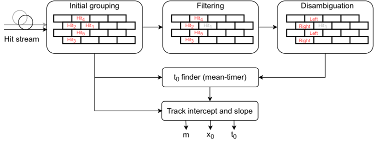
The reconstruction algorithm implements a “hybrid method”: two neural networks are used to filter hits and assign the correct laterality pattern starting from the hits time and channel information. Once the correct hit and laterality combination is found, the mean-timer equation univocally associated with that specific pattern is used to find the track parameters. Without the neural networks, all the possible pairs combination-equation need to be probed, resulting in a large combinatorial. A diagram of the algorithm is shown in Figure 1. The first module of the algorithm, called initial grouping, collects hits from the continuous stream and organizes them in time-coherent $4\times 4$ macro-cells, a set of neighboring cells fully containing all the possible patterns of a muon. Each macro-cell is then fed to the neural network blocks. The first, filtering, retains only the hits produced by the passage of a muon. The hits passing the filtering step are then processed by the disambiguation network, where the correct laterality is predicted. From here, the crossing time $t_{0}$, intercept $x_{0}$, and slope $m$ are computed.
To reduce the FPGA resource utilization, models were trained using QKeras Qkeras sft_qkeras and iteratively pruned during the training phase. Finally, the package HLS4ML HLS4ML fastml_hls4ml was used to produce the High-Level Synthesis code for the models. The inference time of the two neural networks is 2 clock cycles at $40\,$\mathrm{MHz}$$ each, i.e., $50\,$\mathrm{ns}$$. However, the system is a pipeline with an initiation interval of 1, meaning that a new input can be accepted every clock cycle. Moreover, the aim of this stage is to enrich the stream of hits with the reconstructed stubs and not to filter as a trigger would do.

3.2 Data preparation on GPGPUs using Rapids

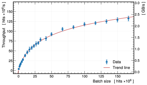
After the reconstruction, all the hits and stubs are transferred to the server memory via DMA. Before being fed to the NPLM algorithm, they need to be aggregated and reformatted. This pre-processing consists mainly of identifying events, e.g., time slices containing muon stubs, filtering spurious hits, and computing new higher-level quantities describing the event. This can be performed leveraging distributed computing frameworks using dataframe-like data structures and operations, as it has been described in 2022NIMPA103666869M . This task can be further accelerated using GPGPUs thanks to CUDA dataframe (cuDF) library implementation in NVIDIA Rapids Rapids . The cuDF library, built on top of Apache Arrow columnar memory format, is used to perform dataframe operations on a GPGPU. Along with dataframes operations, I/O for standard data formats such as Apache Parquet is implemented. Moreover, the basic set of functionalities can also be extended by writing custom kernels using either CUDA or CuPy/Numba. The processing steps used in this work have been easily ported to cuDF, as they consist mainly of simple aggregations, filtering, and column-wise operations. The performance of this pipeline stage can be seen in Figure 2. The time needed to read and process data is measured by changing the batch size, i.e., the number of hits in the dataset processed together. A throughput of over $2\,$\mathrm{G}\mathrm{B}\mathrm{/}\mathrm{s}$$ is achieved when working with large batch sizes of the orders of millions of hits. Getting this amount of data from our test setup using cosmic rays would require running the acquisition for over 2 hour. However, for large experiments, the same amount of data can be collected in seconds. The goal of online processing is to reduce data, i.e., computing a higher level representation of the data, to keep the throughput manageable for the anomaly detection application.

Figure 2: Throughput performance of the preprocessing algorithm in relation to batch sizes, measured in millions of hits. Throughput is quantified in terms of processed hits (left $y$-axis) and gigabytes (right $y$-axis) per second of processing time.

4 Anomaly detection

At large-scale collider experiments, utilizing an unfiltered muon data stream would enable the exploration of yet-unobserved anomalies, which are commonly filtered away by trigger systems. For the purpose of testing the full chain implementation on our small-scale experimental setup, we recast this advantage into a DQM framework, in which detecting anomalies serves as a real-time evaluation metric for the detector’s performance.

4.1 Dataset and anomalies

Following the track reconstruction process, data is transformed from a hit-centric representation to an event-oriented one. Events are thus defined by their four drift timesâone from each layerâand the crossing angle of the muon with the vertical axis. To mimic the most common sources of detector anomaly, we then induced potential malfunctions within the system. By altering the voltage of the cathodic strips and the front-end thresholds, we introduced malfunction scenarios at varying intensities: 75%, 50%, and 25% of their typical operational values. The datasets procured under these anomalous conditions were treated with the same rigorous processing as those obtained under regular conditions. As part of our data acquisition campaign, we systematically gathered information across six distinct configurations, capturing approximately $10^{4}$ events for each setup. Additionally, to establish a robust baseline for comparison, we collected approximately $3\times 10^{5}$ events from the detector’s standard operational conditions. The datasets are further discussed in Ref. DQMpaper .

4.2 Anomaly detection methodology

In data quality monitoring, one aims to assess the operational state of the detector, which has a direct impact on the quality of the data gathered. This evaluation can be formally framed as assessing the alignment of a dataset, denoted as $\mathcal{D}$, with the expected statistical distribution under standard operational conditions, represented as $P(x\,|\,\text{R})$. The direct knowledge of the reference distribution $P(x\,|\,\text{R})$, however, is unavailable. We thus exploit a reference dataset $\mathcal{R}$ that stands in for this distribution. Therefore, our method compares the datasets $\mathcal{D}$ and $\mathcal{R}$ to see if they originate from the same statistical distribution.

In our investigation, we employ a reference dataset of fixed size $\mathcal{N}_{\mathcal{R}}=2000$, extracted from a larger pool of approximately $3\times 10^{5}$ muon data collected under detector conditions labeled as standard. We then monitor batches of varying sizes, $\mathcal{N}_{\mathcal{D}}=250$, $\mathcal{N}_{\mathcal{D}}=500$, and $\mathcal{N}_{\mathcal{D}}=1000$, for all the anomalous configurations reported in Section 4.1.

The NPLM approach

To compare a data batch $\mathcal{D}$ with a reference sample $\mathcal{R}$, we employ the NPLM algorithm DAgnolo:2018cun ; DAgnolo:2019vbw . This algorithm calculates a test statistic by quantifying the log-likelihood ratio between the reference hypothesis and the actual, yet unknown, distribution generating the observed data batches. It does so through a machine-learning model $f_{\mathbf{w}}(x)$, which acts as a universal function approximator parameterized by trainable parameters $\mathbf{w}$. It introduces alternative data distributions $P(x\,|\,\text{H}_{{\mathbf{w}}})$, deviating from $P(x\,|\,\text{R})$ if $\mathcal{D}$ and $\mathcal{R}$ stem from different distributions.

The model $f_{\mathbf{w}}(x)$ can be constructed using either neural network or kernel methods and trained using a weighted logistic loss function. Notably, the Falkon library falkonlibrary2020 sft_falkon significantly enhances the efficiency of kernel methods. This library employs Gaussian kernels with a tunable width $\sigma$. Furthermore, this library introduces several simplifications that enhance computation, especially for GPU-based training. Noteworthy among these is the Nyström approximation, which reduces computational complexity by enabling solutions composed of weighted combinations of selected data points. These points, termed Nyström centers, are randomly chosen from input data. The selection of the number of centers, $M$ ($M\leq\mathcal{N}$), is a hyperparameter demanding careful consideration. For further insights, refer to Ref. falkonlibrary2020 .

Hyperparameter tuning

For hyperparameter selection, we rely exclusively on data from the reference working condition to ensure model independence. The tuning process involves the optimization of the following:

$\,\,1.\,\,$ The number of centers, $M$, which balances model expressiveness and training speed, by seeking the largest $M$ that improves expressiveness without excessive training time.

$\,\,2.\,\,$ The Gaussian width $\sigma$, determined as the 90th percentile of pairwise distances among reference-distributed data points.

$\,\,3.\,\,$ The regularization parameter $\lambda$, minimized while maintaining training stability.

Calibration and p-value extraction

After hyperparameter optimization, the model undergoes training to adapt its parameters $\mathbf{w}$ to approximate observed data. This yields trained parameters $\hat{\mathbf{w}}$ characterizing the best-fit hypothesis $\text{H}_{\hat{\mathbf{w}}}$. The test statistic associated with the log-likelihood ratio for a data batch $\mathcal{D}$ and reference sample $\mathcal{R}$ is then computed as:

$$t(\mathcal{D})=2\sum_{x\in\mathcal{D}}\log\frac{P(x\,|\,\text{H}_{\hat{\mathbf{w}}})}{P(x\,|\,\text{R})}=2\sum_{x\in\mathcal{D}}f_{\hat{\mathbf{w}}}(x)\,.$$ (1)

The numerical value of $t(D)$ has no inherent meaning. To extract physical insights, it has to be calibrated and referenced to the test statistic distribution under the reference hypothesis, $P(t\,|\,\text{R})$. The test statistic calibration proceeds by considering larger positive values of $t$ as more likely if the best-fit alternative distribution $P(x\,|\,\text{H}_{\hat{\mathbf{w}}})$ fits the data better than the reference distribution $P(x\,|\,\text{R})$. This suggests that $\mathcal{D}$ might not adhere to $P(x\,|\,\text{R})$. To estimate $P(t\,|\,\text{R})$ empirically, we generate artificial data batches (termed toy datasets) of the same size $\mathcal{N}_{\mathcal{D}}$ as real data batches, train the model, and compute $t$ for each. By creating histograms of $t$ values from toy datasets, we estimate $P(t\,|\,\text{R})$. Furthermore, considering $P(t\,|\,\text{R})$ approximated by a $\chi^{2}$ distribution, we fit the empirical distribution of $t$ values to obtain a continuous test statistic distribution under reference conditions.

To quantify the discrepancy between $\mathcal{R}$ and $\mathcal{D}$, we calculate the $p$-value:

$$p\,[\,t(\mathcal{D})\,]=\int_{t(\mathcal{D})}^{\infty}\,P(t^{\prime}\,|\,\text{R})\,\text{d}t^{\prime}\,.$$ (2)

The $p$-value measures the likelihood that a reference-distributed batch yields a test statistic value more improbable (i.e., larger) than the observed $t(\mathcal{D})$.

4.3 Results and Performance

Figure 3: Distribution of the test statistic for a data batch size of $\mathcal{N}_{\mathcal{D}}=500$. Grey histograms represent the empirical test statistic distribution $P(t\,|\,\text{R})$. Histograms in shades of red and green are test statistics of anomalous batches corresponding to the cathodes and thresholds anomaly classes, respectively.

Anomaly detection performance

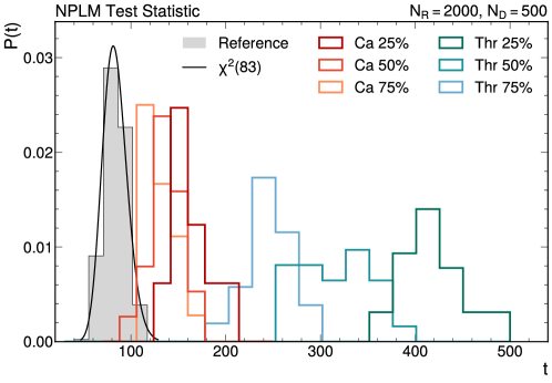
After calibrating the test statistic in Eq. 1 using toy datasets from the standard detector conditions, we sample (without replacement) a few datasets from each anomaly category and fill a histogram of the output $t(\mathcal{D})$ values. Then, we compute the $p$-value of the median of the test statistic distribution using Eq. 2 and a fitted $\chi^{2}$ distribution approximating $P(t\,|\,\text{R})$. Figure 3 shows the NPLM test statistic distribution for the cathodes and thresholds anomalies for the batch size configuration of $\mathcal{N}_{\mathcal{D}}=500$. Further details are available in Ref. DQMpaper .

From these histograms, we observe that the test statistics for anomalous batches, highlighted in Fig. 3 in shades of red and green for the cathodes and thresholds anomaly classes, respectively, are noticeably distinct from the reference distribution. This distinction validates the monitoring algorithm’s capability to identify anomalies. To provide a quantitative measure, we assess the median values of the $t(\mathcal{D})$ distributions corresponding to the 75%, 50%, and 25% anomaly configurations. We find that as the severity increases from 75% to 50% to 25%, the median of the test statistic distribution becomes progressively larger, increasingly diverging from the reference $t$ distribution $P(t\,|\,\text{R})$. This observed trend quantitatively confirms the algorithm’s enhanced sensitivity to anomalies with escalating severity of detector failure.

Training time performance and scalability

(a)

(b)

Figure 4: Left (a): Training time as a function of the training set size $\mathcal{N}$ for the NPLM algorithm. Right (b): Throughput, calculated as the number of muon events divided by the average training time, plotted against the training set size $\mathcal{N}$. Shaded areas represent regions typical for DQM applications and New Physics searches using NPLM.

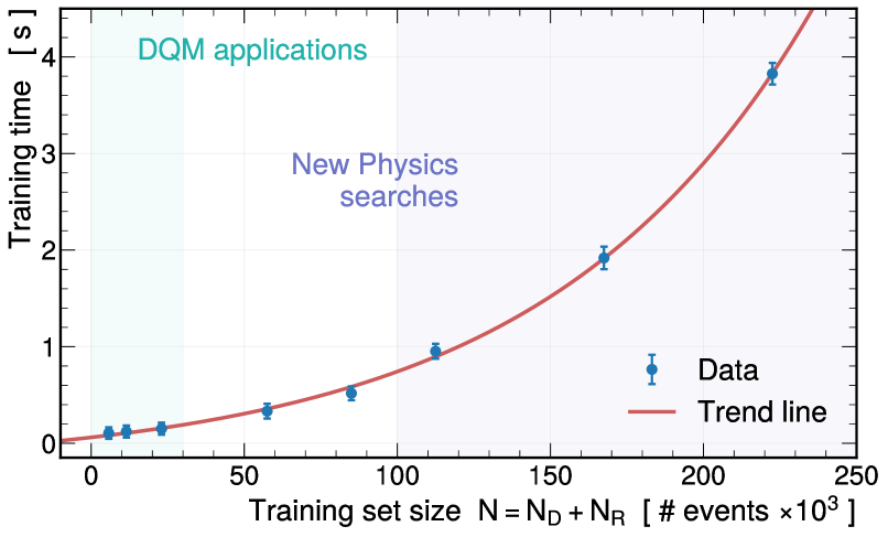
As the natural objective of this work is to extend its deployment to large-scale experiments with significantly higher throughput, it becomes crucial to evaluate the scalability of training execution time. Accordingly, we systematically adjusted $\mathcal{N}_{\mathcal{R}}$ and $\mathcal{N}_{\mathcal{D}}$ to assess the system’s performance in handling larger data batches within a fixed latency. We increased the total event count $\mathcal{N}=\mathcal{N}_{\mathcal{D}}+\mathcal{N}_{\mathcal{R}}$ in the training set, primarily by increasing $\mathcal{N}_{\mathcal{R}}$, while maintaining a relatively stable ratio $\mathcal{N}_{\mathcal{D}}\,/\,\mathcal{N}_{\mathcal{R}}$. Subsequently, we tuned the model hyperparameters for each unique configuration, spanning $\mathcal{N}$ from approximately $2\times 10^{3}$ to $230\times 10^{3}$, employing the same hyperparameter selection procedure. We ran the NPLM algorithm on distinct training sets $\mathcal{O}(1000)$ times for each configuration. We use the average training time as our primary metric. The standard deviation provides additional insights into the variability amongst repeated independent training. This approach provided the training time trend relative to the training set size $\mathcal{N}$, as shown in Figure 4(a). Although the training time follows an exponential trend with respect to $\mathcal{N}$, the absolute values of the training times for the range of batch sizes examined are sufficiently low. This supports the algorithm’s suitability for real-time applications. Additionally, we determined the throughput by dividing the number of analyzed events by the average training time. The throughput as a function of $\mathcal{N}$ is illustrated in Figure 4(b). We observe that the throughput initially increases for smaller batch sizes, peaks in the range of $50\,000$ to $100\,000$ events, and subsequently decreases. Note that the derived metrics for training time and throughput serve as benchmarks that are inherently tied to the particular system configuration and computing infrastructure used in our study.

5 Concluding remarks

The primary objective of this study was the implementation of an online data processing pipeline for anomaly detection on a trigger-less data stream. As a first example, data generated by a muon detector is considered. The pipeline architecture comprises a two-stage data processing flow: an initial local reconstruction executed on an FPGA, followed by data preparation and anomaly detection stages, both benefiting from GPGPU acceleration. We leveraged the New Physics Learning Machine (NPLM) algorithm to create a data quality monitoring application that identifies induced detector malfunctions spanning various severity levels. The effective implementation of the NPLM algorithm for data quality monitoring using unfiltered, high-throughput data streams suggests its applicability to broader research objectives. Specifically, the same computational pipeline can be adapted to search for New Physics phenomena in large-scale, high-energy physics experiments. To enhance the pipeline’s efficiency, several paths for improvement are available. Most notably, future works will focus on streamlining the data flow from the FPGA to the GPU memory by applying zero-copy data transfer models.

References

- (1) D. D’Agostino, D. Cesini, Frontiers in Big Data 4, 652881 (2021)
- (2) The CMS Collaboration, JINST 3, S08004 (2008)
- (3) N. Bartosik, M. Antonelli, O.R. Blanco-Garcia, M. Boscolo, M. Iafrati, B. Ponzio, M. Ricci, M. Rotondo, S. Hoh, D. Lucchesi et al., PoS LeptonPhoton2019, 047 (2019)
- (4) M. Migliorini, J. Pazzini, A. Triossi, M. Zanetti, A. Zucchetta, Journal of Physics: Conference Series 2374 (2021)
- (5) R.T. D’Agnolo, A. Wulzer, Phys. Rev. D 99, 015014 (2019), 1806.02350
- (6) R.T. D’Agnolo, G. Grosso, M. Pierini, A. Wulzer, M. Zanetti, Eur. Phys. J. C 81, 89 (2021), 1912.12155
- (7) S. Baron, J.P. Cachemiche, F. Marin, P. Moreira, C. Soos, Implementing the GBT data transmission protocol in FPGAs, in Topical Workshop on Electronics for Particle Physics (CERN, 2009)
- (8) F. Gasparini, R. Giantin, R. Martinelli, A. Meneguzzo, G. Pitacco, P. Sartori, R. Soggia, P. Zotto, M. Andlinger, F. Szoncso et al., Nuclear Instruments and Methods in Physics Research Section A: Accelerators, Spectrometers, Detectors and Associated Equipment 336, 91 (1993)
- (9) C.N. Coelho, A. Kuusela, S. Li, H. Zhuang, T. Aarrestad, V. Loncar, J. Ngadiuba, M. Pierini, A.A. Pol, S. Summers, Nature Mach. Intell. 3, 675 (2021), 2006.10159
- (10) Google, google/qkeras, https://github.com/google/qkeras
- (11) J. Duarte et al., JINST 13, P07027 (2018), 1804.06913
- (12) FastML Team, fastmachinelearning/hls4ml (2023), https://github.com/fastmachinelearning/hls4ml
- (13) M. Migliorini, J. Pazzini, A. Triossi, M. Zanetti, A. Zucchetta, Nuclear Instruments and Methods in Physics Research A 1036, 166869 (2022), 2111.05155
- (14) RAPIDS Development Team, RAPIDS: Libraries for End to End GPU Data Science (2023), https://rapids.ai
- (15) G. Grosso, N. Lai, M. Letizia, J. Pazzini, M. Rando, L. Rosasco, A. Wulzer, M. Zanetti, Machine Learning: Science and Technology 4, 035029 (2023)
- (16) G. Meanti, L. Carratino, L. Rosasco, A. Rudi, 33, 14410 (2020), 2006.10350
- (17) FalkonML, Falkonml/falkon, https://github.com/FalkonML/falkon