An Efficient Framework for Global Non-Convex Polynomial Optimization with Nonlinear Polynomial Constraints

Abstract

We present an efficient framework for solving constrained global non-convex polynomial optimization problems. We prove the existence of an equivalent nonlinear reformulation of such problems that possesses essentially no spurious local minima. We show through numerical experiments that polynomial scaling in dimension and degree is achievable for computing the optimal value and location of previously intractable global constrained polynomial optimization problems in high dimension.

The first author acknowledges support by the NSF Graduate Fellowship under Grant No. 2141064.

1 Introduction

Polynomial optimization is a longstanding important problem in applied mathematics due to the number of applications to which it may be applied (e.g. (Zhening2012Approx, , Chapter 4)). Work by Shor shor1987class , Nesterov nesterov2000squared , Parrilo parrilo2000structured and Lasserre lasserre2001global has provided tools for polynomial optimization exploiting polynomial structure to provide methods more specialized than general nonlinear programming. In this work, we aim to make such attempts at polynomial optimization more practical.

We focus on polynomial optimization over the hypercube. Let $p,\{g^{(j)}\}_{j=1}^{J}$ be polynomials in $D$ variables and of degree at most $d$. We consider the constrained non-convex polynomial optimization problem

$$\min_{x\in[-1,1]^{D}} \;\;p(x)$$ (1)

$$\mathrm{subject\,to} \;\;g^{(j)}(x)\geq 0,\,j=1,...,J$$

A framework for efficiently solving unconstrained polynomial optimization over the hypercube was proposed in Letourneau2023unconstrained . Using inspiration from the ideas of Lasserre lasserre2001global , the authors demonstrated how such problems may be efficiently reformulated as problems involving a nonlinear objective over a convex cone of semi-definite matrices in $O(D\cdot d^{2})$ dimensions such that the reformulation possesses no spurious local minima (i.e., essentially every local minimum is a global minimum).

This paper generalizes the reformulation presented in Letourneau2023unconstrained to the case of constrained polynomial optimization problems over semi-algebraic sets. Our generalized reformulation (14) is similar to that of Letourneau2023unconstrained with the addition of $2J$ scalar constraints. This reformulation has similar guarantees. We have implemented an algorithm for solving the generalized reformulation in the Julia programming language from which we have produced promising numerical results.

Our contributions can be summarized as follows.

• Efficient reformulations of constrained polynomial optimization A reformulation of (1) is introduced. The reformulation has a nonlinear objective, with a feasible region consisting of the intersection of the cone of semidefinite matrices with a region determined through scalar nonlinear constraints. The reformulation is equivalent to the original problem in the sense they share optimal value (Theorem 2) and optimal locations up to a canonical transformation (Theorem 3). The reformulation may be solved to optimality using descent techniques (due to the absence of local minima), something generally not possible using the original formulation.

• Efficient characterization of product measures over semi-algebraic subsets of $[-1,1]^{D}$ We give a complete and efficient characterization of the set of product measures supported over the set,

  $$\left\{x\in[-1,1]^{D}\,:\,g^{(j)}(x)\geq 0,\,j=1,...,J\right\}$$

  via the moments of the measures using semidefinite and scalar nonlinear inequality constraints (Proposition 1).

The remainder of this paper is structured as follows: Previous work is discussed in Section 1.1. Section 2 introduces notation, theory, and our novel generalized reformulation of (1). Section 3 discusses algorithmic and technical aspects of our solver implementation in the Julia programming language. Section 4 presents numerical results demonstrating correctness and performance of our framework. Section 5 presents conclusions and a discussion of future work. Proofs can be found in Appendix A.

1.1 Previous Work

While there are other approaches to polynomial optimization, this work relies heavily on the moment formulation for polynomial optimization emphasized by Lasserre lasserre2001global . The moment formulation and its dual were connected to semidefinite programming (SDPs) by lasserre2001global and parrilo2000structured , which opened the door for practical computations.

The idea of the moment formulation is as follows: instead of evaluating polynomials directly, the optimization is done over measures. The values of the objective and constraints are the integrals over the multidimensional measures, the moments of which are the integrals of the monomials in the original polynomial objective. Using a finite-size semidefinite constraint to characterize a measure is necessary but not sufficient to ensure the moments actually come from a true measure. Therefore, the SDP provides a relaxation to the original problem. The primary advantage of this approach is that the resulting problem is convex and can be solved relatively efficiently. However, rather than provide an exact reformulation, lasserre2001global results in a convex relaxation, where the solution provides a lower bound on the optimal minimum. The quality of this bound depends on the degree of the Sums-Of-Squares (SOS) doi:10.1137/040614141 ; prajna2002introducing polynomials used to generate the relaxation. Better relaxations increase the size of the resulting SDP, adversely affecting scaling. In lasserre2001global ; Parrilo2003 it was demonstrated that any sequence of problems of increasing size (“SOS degree”) will eventually converge to an exact solution in finite time (the sequence of problems is known as the “Lasserre Hierarchy”). Although the hierarchy has been found to converge relatively rapidly on some specific problems (see, e.g., de2022convergence ), theoretical estimates indicate that super-exponential sizes are required in the worst case Klerk2011 .

The poor theoretical scaling arises from the underlying real algebraic geometry. Degree estimates for the approach of lasserre2001global rely on results by Putinar putinar1993positive and Nie and Schweighofer nie2007complexity . These results express positive polynomials over compact semi-algebraic subsets of Euclidean spaces through SOS-like representations of finite degree. They demonstrate that this can be done in any dimension; however, their estimates demand a super-exponential SOS degree of the original problem in both dimension and degree, resulting in estimates suggesting intractable cost for solving polynomial optimization problems using lasserre2001global ’s framework in the general case.

The work of Letourneau2023unconstrained proposed a modification of lasserre2001global to improve scaling for the case of polynomial optimization over the hypercube. Instead of optimizing over general measures, they restrict to a sub-class of measures (the convex combination of product measures). The advantage is that characterizing such measures requires significantly smaller semidefinite constraints. The disadvantage is that the problem is no longer convex. Nonetheless, they show that there is generically always a descent direction starting from any non-optimal feasible point.

Our work consists in a non-trivial generalization of the ideas in Letourneau2023unconstrained to the case of polynomial optimization over the intersection of a general semi-algebraic set and the hypercube. Our framework and results overcome the drawbacks of lasserre2001global in the context of constrained polynomial optimization by once again restricting the space of feasible measures. We show this restricted space can be represented efficiently in Proposition 1. In particular, we provide an explicit efficient characterization of the set of product measures supported over,

$$\left\{x\in[-1,1]^{D}\,:\,g^{(j)}(x)\geq 0,\,j=1,...,J\right\}.$$

In this generalized reformulation, we preserve the guarantees provided by Letourneau2023unconstrained . Our conclusions about efficiency are much stronger than the general case considered in lasserre2001global and highlight the practicality of our generalized reformulation.

2 Theory

Let $p,\{g^{(j)}\}_{j=1}^{J}$ be polynomials in $D$ variables and of degree at most $d$. We consider the constrained non-convex polynomial optimization problem,

$$\min_{x\in[-1,1]^{D}} \;\;p(x)$$

$$\mathrm{subject\,to} \;\;g^{(j)}(x)\geq 0,\,j=1,...,J.$$

2.1 Preliminaries

Polynomials

Let the dimension of (1) be $D$, and let $d$ be the problem degree (i.e., the maximum degree of the objective and constraint polynomials). A $D$-dimensional multi-index $n=(n_{1},n_{2},...,n_{D})$ is a $D$-tuple of nonnegative integers. Let $\lvert n\rvert=\sum_{i=1}^{D}n_{i}$ be the multi-index degree. A monomial is written as

$$x^{n}=\prod_{i=1}^{D}x_{i}^{n_{i}}.$$ (2)

Unless otherwise stated, all polynomials are written in the monomial basis. The vector space of polynomials of degree $d$ in dimension $D$ is denoted $\mathbb{P}_{D,d}$, i.e.,

$$\mathbb{P}_{D,d}:=\left\{\sum_{\begin{subarray}{c}\lvert n\rvert\leq d\\ \,n\in\mathbb{N}^{D}\end{subarray}}\,p_{n}\,x^{n}:\,p_{n}\in\mathbb{R}\right\},$$ (3)

where the summation is over all multi-indices of degree less than or equal to $d$. In particular, note that $\mathbb{P}_{D,d}$ has dimension

$$\#\{n\in\mathbb{N}^{D}\,:\,\lvert n\rvert\leq d\}=\binom{D+d}{d}\leq\min\left(D^{d},d^{D}\right).$$ (4)

Hence, for a fixed degree $d$, the dimension of the vector space of polynomials $\mathbb{P}_{D,d}$ grows polynomially in the problem dimension $D$. The notation $\mathbb{P}_{D,\infty}$ is used to represent polynomials of any finite degree. The support of a polynomial $p\in\mathbb{P}_{D,\infty}$ corresponds to the locations of its nonzero coefficients; i.e.,

$$\mathrm{supp}(p):=\{n\in\mathbb{N}^{D}\,:\,p_{n}\not=0\},$$ (5)

and the cardinality (number of elements) of the support is denoted by

$$N_{p}:=\#\,\mathrm{supp}(p).$$ (6)

Moments of measures

The set of regular Borel measures over $\mathbb{R}^{D}$ (cohn2013measure ) is denoted as $\mathbb{B}_{D}$, and the support of a measure $\mu(\cdot)\in\mathbb{B}_{D}$ is designated by $\mathrm{supp}(\mu(\cdot))$. It represents the smallest set such that $\mu\left(\mathbb{R}^{D}\backslash\mathrm{supp}(\mu(\cdot))\right)=0$. For a fixed multi-index $n$, a $D$-dimensional Borel measure in $\mathbb{B}_{D}$ has an $n^{th}$ moment defined to be the multi-dimensional Lebesgue integral,

$$\mu_{n}:=\int_{\mathbb{R}^{D}}x^{n}\,\mathrm{d}\mu(x).$$ (7)

When referring to a measure, parentheses are employed (e.g., $\mu(\cdot)$). If the parentheses are absent (e.g., $\mu$), we are referring to a vector of moments associated with the measure. Let $X_{i}$ be measureable subsets of $\mathbb{R}$. A regular product measure is a regular Borel measure of the form

$$\mu(X_{1}\times\cdots\times X_{D})=\prod_{i=1}^{D}\mu_{i}(X_{i}),$$ (8)

where each factor $\mu_{i}(\cdot)$ belongs to $\mathbb{B}_{1}$. In this context, the moments of a product measure up to degree $d$ correspond to a $D$-tuple of real vectors $(\mu_{1},\mu_{2},...,\mu_{D})\in\mathbb{R}^{(d+1)\times D}$, where each element is defined as

$$\mu_{i,n_{i}}:=\int_{\mathbb{R}}x_{i}^{n_{i}}\,\mathrm{d}\mu_{i}(x_{i}).$$ (9)

The vectors $\mu_{i}$ refer to the vector of moments of the 1D measure $\mu_{i}(\cdot)$. With a single sub-index, $\mu_{i}\in\mathbb{R}^{d+1}$ represents the vector of moments, and with two sub-indices, $\mu_{i,n_{i}}\in\mathbb{R}$ represents scalar moments (vector elements) of a 1D measure. In this work, we are interested in collections of $L$ measures that are each products of 1D measures. All of those moments are represented by the $(d+1)\times D\times L$ real numbers $\mu=\{\mu_{i}^{(l)}\}_{l,i}$. Finally, we introduce the following notation to represent the moments of sums of product measures,

$$\phi_{n}(\mu)=\sum_{l=1}^{L}\prod_{i=1}^{D}\mu^{(l)}_{i,n_{i}}$$ (10)

Moment matrices

Let $\mu_{i}$ be a sequence of moments of a 1D measure. The degree-$d$ 1D moment matrix (or moment matrix) associated with a polynomial $h\in\mathbb{P}_{1,d^{\prime}}$ is defined to be the $(d+1)\times(d+1)$ matrix $\mathcal{M}_{d}(\mu_{i},h(x_{i}))$ with entries,

$$[\mathcal{M}_{d}(\mu_{i},h(x_{i}))]_{m,n}=\int h(x_{i})\,x_{i}^{m+n}\,\mathrm{d}\mu_{i}(x_{i})=\sum_{k_{i}=0}^{d^{\prime}}h_{k_{i}}\,\mu_{k_{i}+m+n},$$ (11)

for $0\leq m,n\leq d$. When $g(\cdot)\equiv 1$, we use the short-hand notation,

$$\mathcal{M}_{d}(\mu_{i}\mathchar 24635\relax\;1)=\mathcal{M}_{d}(\mu_{i}).$$ (12)

The construction of such matrices requires the knowledge of only the first $2d+d^{\prime}+1$ moments of $\mu_{i}(\cdot)$, i.e., $\{\mu_{i,n}\}_{n=0}^{2d+d^{\prime}}$.

2.2 Reformulation on the hypercube

This section summarizes results presented in Letourneau2023unconstrained that underly this work. In Letourneau2023unconstrained , problems of the form,

$$\min_{x\in[-1,1]^{D}}\,p(x),$$ (13)

were treated. That work proposed the following reformulation

$$\min_{\mu\in\mathbb{R}^{(d+1)\times D\times L}} \;\;\sum_{n\in\mathrm{supp}(p)}\,p_{n}\,\phi_{n}(\mu)$$ (14)

$$\mathrm{subject\,to} \;\;\mathcal{M}_{d}(\mu^{(l)}_{i})\succeq 0,$$

$$\;\;\mathcal{M}_{d-1}(\mu^{(l)}_{i}\mathchar 24635\relax\;\,1-x_{i}^{2})\succeq 0,\;$$

$$\;\;\mu^{(l)}_{i,0}\geq 0,$$

$$\;\;\phi_{(0,...,0)}(\mu)=1,$$

where the moments $\phi_{n}(\mu)$ are defined in Equation 10 and the constraints are over all $i=1,\dots,D$ and $l=1,\dots,L$. It was shown in Letourneau2023unconstrained that the reformulated problem is equivalent to the original – they share the same global optimal value and locations (under a canonical correspondence). This paper presents a generalization of this reformulation, where polynomial constraints are added to Problem 13 to reformulate Problem 1 (Section 2.3).

The proof of the aforementioned equivalence relies heavily on (Letourneau2023unconstrained, , Proposition 1), which states that to every element in the feasible set of Problem 14, there exists a corresponding Borel measure with moments $\{\phi_{n}(\mu)\}$ for all $0\leq n_{i}\leq d$, i.e., that the multi-dimensional moment problem can be solved efficiently when sums of product measures are concerned.

One contribution of this paper is a generalization of Proposition 1 from Letourneau2023unconstrained , expanding the result to the moment problem over semi-algebraic subsets of $[-1,1]^{D}$. This result is stated in Proposition 1.

2.3 Generalized reformulation for polynomial constraints

We now present the generalized reformulation. Let $\{y_{j}\}_{j=1}^{J}$ be $J$ additional (slack) variables. We re-express the polynomial constraint $g^{(j)}(x)\geq 0$ as

$$\left(g^{(j)}(x)-y_{j}\right)^{2}=0\qquad\text{and}\qquad\;y_{j}\geq 0.$$ (15)

The first constraint is enforced by requiring

$$\int\left(g^{(j)}(x)-y_{j}\right)^{2}\mathrm{d}\mu(x)=0$$ (16)

because then the support of $\mu$ is contained in the feasible set. The formal statement and proof showing this claim is presented in the Appendix in Proposition 6. For $y_{j}$ fixed, the left hand side is a degree-$2d$ polynomial in $x$. Let $\gamma^{(j)}(y_{j})$ be the vector of coefficients in the monomial basis of that polynomial. The reformulated problem is then

$$\begin{split}\min_{\mu\in\mathbb{R}^{(d+1)\times D\times L}}&\;\;\sum_{n\in\mathrm{supp}(p)}\,p_{n}\,\phi_{n}(\mu)\\ \mathrm{subject\,to}&\;\;\mathcal{M}_{d}(\mu^{(l)}_{i})\succeq 0,\\ &\;\;\mathcal{M}_{d-1}(\mu^{(l)}_{i}\mathchar 24635\relax\;\,1-x_{i}^{2})\succeq 0,\;\;\;\\ &\;\;\gamma^{(j)}(y_{j})\cdot\phi(\mu)=0\\ &\;\;y_{j}\geq 0\\ &\;\;\mu^{(l)}_{i,0}\geq 0,\\ &\;\;\phi_{(0,...,0)}(\mu)=1,\end{split}$$ (17)

where the constraints are over all $i=1,\dots,D$, $l=1,\dots,L$, and $j=1,\dots,J$.

This reformulated problem is equivalent to Problem 1 in that it shares the same optimal value and optimal locations under a canonical map (see Theorem 2 and Theorem 3). These results are a consequence of the following proposition (see Appendix A for proofs), which states that for any moment vector satisfying the constraints of the reformulation, there is a measure whose support is contained in the original feasible region.

Proposition 1.

Let $D,d\in\mathbb{N}$ and $(\mu_{1},\mu_{2},...,\mu_{D})\in\mathbb{R}^{(d+1)\times D}$ be such that for each $i=1,...,D$, $\mu_{i,0}=1$, and

$$\mathcal{M}_{d}(\mu_{i}) \succeq 0,$$

$$\mathcal{M}_{d-1}(\mu_{i}\mathchar 24635\relax\;1-x_{i}^{2}) \succeq 0.$$

If in addition for every $j=1,...,J$ there exists some $y_{j}\geq 0$ such that,

$$\gamma^{(j)}(y_{j})\cdot\phi(\mu)=0,$$ (18)

where $\gamma^{(j)}(y_{j})$ is the vector of polynomial coefficients or $\left(g^{(j)}(x)-y_{j}\right)^{2}$, then there exists a regular Borel product measure,

$$\mu(\cdot):=\prod_{i=1}^{D}\mu_{i}(\cdot),$$

supported over the semi-algrbraic set

$$\mathcal{S}:=\cap_{j=1}^{J}\left\{x\in[-1,1]^{D}\,:\,g^{(j)}(x)\geq 0\right\}$$ (19)

such that $\mu\left(\mathcal{S}\right)=1$ and matches the given moments. That is, for all multi-indices $n\in\mathbb{N}^{D}$ such that for every $i=1,\dots,D$, $0\leq n_{i}\leq d$, we have

$$\int_{[-1,1]^{D}}\,x^{n}\,\left(\prod_{i=1}^{D}\mu_{i}(x_{i})\right)\,\mathrm{d}x=\prod_{i=1}^{D}\mu_{i,n_{i}}.$$

The equivalence of the generalized formulation with Problem 1 carries verbatim from Letourneau2023unconstrained as stated in the following theorems. The first theorem states that the global minima is unchanged, and the second theorem provides a global optimality characterization.

Theorem 2.

Problem 1 and Problem 17 share the same global minimum value.

Theorem 3.

Let $\left\{\mu_{i}^{(0)},\mu_{i}^{(1)}\right\}_{i=1}^{D}\in\mathbb{R}^{(2d+1)\times D\times 2}$ be a feasible point of Problem 14 corresponding to a local minimum, and let $\alpha^{(j)}=\prod_{i=1}^{D}\mu^{(j)}_{i,0}$ for $j\in\{0,1\}$. Then, such a point is a global minimum if and only if either

$$\alpha^{(0)}\not=0 \text{ and }\qquad\left\{\frac{\prod_{i=1}^{D}\mu^{(0)}_{i,n_{i}}}{\alpha^{(0)}}\right\}_{\lvert n\rvert\leq d}\text{ is a local minimum, or}$$ (20)

$$\alpha^{(1)}\not=0 \text{ and }\qquad\left\{\frac{\prod_{i=1}^{D}\mu^{(1)}_{i,n_{i}}}{\alpha^{(1)}}\right\}_{\lvert n\rvert\leq d}\text{ is a local minimum.}$$

The previous two theorems are stated here without proof because the steps are the same as the proof for the unconstrained case. We refer the reader to Letourneau2023unconstrained for the unconstrained proof. The only differences are that the set $\mathcal{F}_{L}$ in (A17) should be redefined to be the feasible set of Problem 17 and $\mathcal{S}_{L}$ in (A18) should be a set of sums of product measures supported over level sets of the semi-algebraic set $\mathcal{S}$ (Eq.(19)) .

3 Algorithm and Implementation

In this section, we briefly describe how we numerically solve the generalized reformulated problem (Problem 17) presented in Section 2.3. The reformulation consists of a nonlinear semidefinite program, i.e., an optimization problem with a nonlinear objective, semi-definite constraints and additional linear and nonlinear scalar constraints. After describing how we handle the semidefinite constraints, we provide some details on our software implementation.

Semi-definite constraints are denoted by: $\mathcal{M}\succeq 0$. Within our numerical implementation, we handle semi-definite constraints using the Burer-Monteiro (BM) method burer2003nonlinear , which enforces them through equality constraints of the form: $\mathcal{M}_{d}=XX^{T}$ for some $X\in\mathbb{R}^{(d+1)\times r}$. In our case, the rank $r$ was generally chosen to be $r=d+1$ (full rank). The use of the BM method comes at the cost of introducing (second-order) nonlinearities, but such a reformulation does not change the feasible set when the rank is chosen as such. Further, Boumal et al. boumal2016non have shown that when the rank of a solution is sufficiently small, every second-order stationary point arising under the BM framework corresponds to a global minimum.

With this choice, the reformulation becomes

$$\begin{split}\min_{\mu\in\mathbb{R}^{(d+1)\times D\times L}}&\;\;\sum_{n\in\mathrm{supp}(p)}\,p_{n}\,\phi_{n}(\mu)\\ \mathrm{subject\,to}&\;\;\mathcal{M}_{d}(\mu^{(l)}_{i})=X_{i}X_{i}^{T}\\ &\;\;\mathcal{M}_{d-1}(\mu^{(l)}_{i}\mathchar 24635\relax\;\,1-x_{i}^{2})=Y_{i}Y_{i}^{T}\\ &\;\;X_{i}\in\mathbb{R}^{(d+1)\times(d+1)},\;Y_{i}\in\mathbb{R}^{d\times d}\\ &\;\;\gamma^{(j)}(y_{j})\cdot\phi(\mu)\leq 0\\ &\;\;y_{j}\geq 0,\;\;\;\;\;\;\;\;\;i=1,...,D,l=1,...,L,j=1,...,J\\ &\;\;\mu^{(l)}_{i,0}\geq 0,\\ &\;\;\phi_{(0,...,0)}(\mu)=1,\\ &\;\;\phi_{n}(\mu)=\sum_{l=1}^{L}\prod_{i=1}^{D}\mu^{(l)}_{i,n_{i}}.\end{split}$$ (21)

In this formulation, we replaced the equality in $\gamma^{(j)}(y_{j})\cdot\phi(\mu)=0$ by the inequality $\leq 0$. These are equivalent mathematically because the integral this dot product represents must be nonnegative by construction of $\gamma$ and $\mu$, so a nonnegative quantity that is also nonpositive must be zero.

This problem now only contains scalar equality and inequality constraints, and is therefore more amenable to existing numerical solvers. Table 1 describes the computational cost associated with the evaluation of the objectives and constraints. Note that this cost is at most polynomial in dimension and degree.

Expression	Size	Eval. Cost
$\sum_{n\in\mathrm{supp}(p)}\,p_{n}\,\phi_{n}(\mu)$	$1$	$O\left(N_{p}\,L\,D\right)$
$\mathcal{M}_{d}\left(\mu^{(l)}_{i}\right)$	$(d+1)\times(d+1)$	$O\left(L\,D\,d^{2}\right)$
$\mathcal{M}_{d-1}\left(\mu^{(l)}_{i}\mathchar 24635\relax\;\,1-x_{i}^{2}\right)$	$d\times d$	$O\left(L\,D\,d^{2}\right)$
$XX^{T}$, $YY^{T}$	$O(d)\times O(d)$	$O\left(d^{3}\right)$
$\sum_{l=1}^{L}\prod_{i=1}^{D}\mu^{(l)}_{i,0}-1$	$1$	$O\left(L\,d\right)$
$\gamma^{(j)}(y_{j})\cdot\phi(\mu)$	$J$	$O\left(\max_{j}N^{2}_{g^{(j)}}\,J\,D\right)$

Table 1: Size and evaluation costs of each component of the proposed generalized reformulation.

To solve this problem numerically, we implemented a solver in the Julia programming language bezanson2012julia . For optimization purposes, we used the Nonconvex.jl package Tarek2023nonconvex . This package provides a convenient interface that connects to many backend solvers and is well-suited for the treatment of nonlinear equalities and inequalities.

For the backend solver, we chose to use the ipopt algorithm implementation wachter2006implementation with first-order approximation. We used default parameter values, with the exception of the overall convergence tolerance, which corresponds to the maximum scaled violation under the KKT formulation (i.e., Eq.(6), Wachter2006ip), that we set to $\epsilon=10^{-2}$.

Polynomials found in the objectives and the constraints were represented using the DynamicPolynomials.jl Julia package legat2021polynomials which offers an efficient symbolic way of expressing such functions. Finally, to compute the gradient information required by the ipopt algorithm, we used the Forwarddiff.jl Julia package RevelsLubinPapamarkou2016 which implements automatic differentiation.

4 Numerical experiments

In this section, we present numerical results demonstrating our proposed algorithm and software. To display the versatility and power of our technique, we consider two families of constrained polynomial optimization problems that highlight the hurdles often encountered using traditional descent methods. Our reformulation overcomes these challenges. These include: local minima, non-convexity and disconnected feasible regions. The first family is treated in Section 4.1 and consists of a concave quadratic objective over a connected non-convex feasible set, resulting in two (2) local minima within the feasible region regardless of dimension (see Figure 1). The second family is discussed in Section 4.2. It involves a concave (non-convex) objective over a feasible region consisting of exponentially many disjoint sets (see Figure 5).

To demonstrate the difference between the traditional and reformulated approach, we used a single nonlinear interior point solver (ipopt) to solve the problem both in its original form (Eq.(1)) as well as its reformulated form (Eq.(21)). We show below that while the original formulation suffers from non-convexity and generally fails to find a global optimum, the reformulated approach consistently succeeds (Tables 2 and 3).

4.1 Elliptical Annulus

Problem setup

For our first numerical experiments, we consider the problem of minimizing a concave quadratic objective over a feasible region consisting of an (non-convex) elliptical annulus as shown in Figure 1. The feasible region is constructed as follows: given the dimension $D$ of the problem, we construct a diagonal matrix,

$$M=\begin{pmatrix}1&0&0&\cdots&0\\ 0&M_{2}&0&\cdots&0\\ \vdots&\vdots&\vdots&\ddots&\vdots\\ 0&0&0&\cdots&M_{D}\end{pmatrix}$$

where $M_{2},M_{3},\dots,M_{D}$ are sampled independently from a uniform distribution over $[\epsilon,1]$ for some small $\epsilon>0$. Then, after fixing $0<c<1$, the problem is

$$\min_{x\in\mathbb{R}^{D}} \qquad p(x):=-(x_{1}-0.1)^{2}$$ (22)

s.t. $$\qquad x^{T}Mx\leq 1$$

$$\qquad x^{T}Mx\geq c$$

$$\qquad-1\leq x_{i}\leq 1\;\;\forall i.$$

An illustration of the problem when $D=2$ and $c=\frac{2}{3}$ is presented in Figure 1.

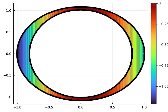
Figure 1: Representation of Problem 22 in two dimensions (2D) with $c=\frac{2}{3}$. The feasible region consists in a non-convex elliptical annulus. The objective is concave in the first dimension and possesses two (2) loca minima over the feasible set.

In any given dimension $D$, the problem contains exactly two (2) local minima, only one of which is a global minimum located at $x^{*}=(-1,0,\dots,0)$ with value: $p(x^{*})=-1.21$. Within the non-convex feasible region, there are two (2) basins of attractions (corresponding to the two local minima) of roughly equal volume. We thus expect traditional descent methods with a starting point uniformly chosen within the feasible region to succeed at most $50\%$ of the time.

Numerical results

For our numerical experiments, we fixed $c=\frac{10}{11}$ and solved four (4) instances of Problem (22) with different random starting points for each dimension $D\in\{2,\dots,32\}$. The results are reported below.

Figure 2 shows the average (over $4$ instances) optimal objective value error for each dimension under consideration. It can be seen that the reformulation succeeds in finding the global minimum value in every instance; the error is on average under $10^{-5}$ which is below the expected bound (using an overall convergence tolerance of $\epsilon=10^{-2}$). Figure 3 further shows the value of the active constraint ($g(x)=1-x^{T}Mx$) at optimality. A positive value indicates feasibility, and we see that no solution is more than approximately $10^{-3}$ away from positivity. This is within the solver accuracy parameter and indicates numerical feasibility.

Figure 2: Average relative errors in elliptical annulus problem. The error is on average approximately $10^{-5}$ and lies below the solver threshold ($10^{-2}$) regardless of the dimension $D$.

Figure 3: Average error of the active constraint in elliptical annulus problem. The computed solution has an average error of roughly $-10^{-3}$ and is numerically feasible regardless of the dimension $D$.

The average wall time taken by our numerical solver (Section 3) for computing the solution of the aforementioned problems is shown in Figure 4. We observe polynomial scaling with dimension. This is in line with expectations (see Table 1). Indeed, as discussed in Section 2.3, the efficiency of our scheme is such that the reformulated problem lies in a space for which dimension grows slowly (linearly) with the dimension of the underlying problem. In this sense, the most expensive computations involve the evaluation of the objective, the gradients and their respective constraints. In this context, the cost scales like $O(D^{2})$ (we do not leverage the sparsity of $M$ in our implementation), which is nearly the observed scaling in Figure 4.

Figure 4: Average wall times of solving reformulated elliptical annulus problem using our novel formulation (solid line). The dotted line indicates a scaling of $O(D^{2})$.

Comparison with original formulation

To demonstrate the superior characteristics of our reformulation, we compare it to the results obtained using the original formulation. For this purpose, we used an existing, robust solver commonly used for nonlinear optimization: ipopt wachter2006implementation . We use the latter to solve the original formulation (Problem 1) directly within an overall convergence tolerance of $10^{-2}$. We used the same solver for the reformulated problem (Problem 21). In the event that ipopt returned a failure code for either formulation, the problem was thrown out. Table 2 displays the proportion of problems for which the global optimum was found for our scheme (center column) and using the original formulation (right column) as a function of dimension. As can be observed, our approach succeeds consistently, while the original formulation fails approximately $50\%$ of the time. As discussed previously, this is expected given the geometry of the problem which possesses two basin of attractions around two local minima, only one of which is also global. This is a problem that plagues all solver based on local descent when the problem is not convex or possesses more than one local minimum with different values. In this case, local descent solvers (including ipopt) may only find local minima which lie within the basin of attraction of the starting point. In our case, we used a random initialization as is commonly done, and run the same problem $4$ times with with a different starting point. The existence of two basins of attractions with of roughly equals size explains the average $50\%$ success rate of the original formulation. By contrast, our proposed reformulation does not suffer from this drawback since the reformulated problem does not possess spurious local minima.

$D$	Reformulation	Original
$2$	$100$%	$75$%
$3$	$100$%	$75$%
$4$	$100$%	$0$%
$5$	$100$%	$50$%
$6$	$100$%	$25$%
$7$	$100$%	$50$%
$8$	$100$%	$100$%
$9$	$100$%	$66.67$%
$10$	$100$%	$50$%
$11$	$100$%	$33.33$%
$12$	$100$%	$66.67$%
$13$	$100$%	$0$%
$14$	$100$%	$75$%
$15$	$100$%	$0$%
$16$	$100$%	$0$%
$17$	$100$%	$25$%
$18$	$100$%	$0$%
$19$	$100$%	$66.67$%
$20$	$100$%	$66.67$%
$21$	$100$%	$75$%
$22$	$100$%	$33.33$%
$23$	$100$%	$0$%
$24$	$100$%	$25$%
$25$	$100$%	$100$%
$26$	$100$%	$50$%
$27$	$100$%	$66.67$%
$28$	$100$%	$100$%
$29$	$100$%	$100$%
$30$	$100$%	$33.33$%
$31$	$100$%	$75$%
$32$	$100$%	$33.33$%

Table 2: Proportion of problems for which our approach (our reformulation, center) and the original formulation (right) find the global minimum of the elliptic annulus problem (Problem 22) within an error of $10^{-2}$. Every problems was solved $4$ times using ipopt as backend, and if ipopt returned an error code for either formulation, then the instance was thrown out.

4.2 Disconnected Feasible Region

Problem setup

For our second numerical experiment, we chose a more complex family of problems which can be described as follows. Let

$$c(x)=1-\frac{x^{2}}{2}+\frac{x^{4}}{24},$$ (23)

which corresponds to the first three terms of the Taylor expansion of $\cos(x)$ around the origin. Then the family of problems may be written as

$$\min_{x\in\mathbb{R}^{D}} \qquad p(x):=-\sum_{i=1}^{D}(x_{i}+0.1)^{2}$$ (24)

s.t. $$\qquad c(\pi x_{i})\cdot c(\pi x_{j})\geq 10^{-2}\;\forall\,i\not=j$$

$$\qquad-1\leq x_{i}\leq 1\;\;\forall i.$$

The objective and feasible region are depicted in Figure 5.

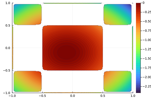
Figure 5: Two dimensional version of disjoint patches problem.

The objective is a concave quadratic function, while the feasible region is comprised of a number of disconnected regions (disjoint patches). Each region possesses at least one local minimum, and there are more than $2^{D}$ such regions in dimension $D$. The true global minimum of Problem (24) is located at $x^{*}=(1,1,\dots,1)$ and has value: $p(x^{*})=1.21\cdot D$.

Numerical results

We carried out numerical experiments where we solved four (4) instances of Problem (24) in both the reformulated and oririnal forms, with different uniformly random starting points for dimensions $D\in\{2,\dots,14\}$. In the event that ipopt returned a failure code for either formulation, the problem was thrown out. We discuss the results below.

First, Figure 6 shows the objective error found by the reformulated problem as a function of dimension. Note that the error is consistently below $10^{-2}$ which is within the solver tolerance. This shows that our reformulation-based solver is indeed correct and solves Problem (24) in every instance regardless of dimension. Figure 7 also shows the value of the active constraint ($g(x)=\min_{i\not=j}\,\left(c(\pi x_{i})\cdot c(\pi x_{j})-10^{-2}\right)$) at optimality. A positive value indicates feasibility, and we see that all values are indeed positive. This indicates that the computed solution is numerically feasible and on the boundary of the feasible set, as expected.

Figure 6: Average relative objective errors in disjoint patches problem. The error is on average approximately $10^{-5}$ and lies below the solver threshold ($10^{-2}$) regardless of the dimension $D$.

Figure 7: Maximum relative errors for active constraint in disjoint patches problem. The computed solution has an average error of roughly $10^{-2}$ and is numerically feasible regardless of the dimension $D$.

Finally, Figure 8 shows scaling results. In particular, we observe a polynomial scaling as a function of dimension corresponding to $D^{4}$. This is in line with the most expensive operations in Table 1 which in this case corresponds to the evaluation of $J=O(D^{2})$ constraints, each of which has $\max_{j}N_{g^{(j)}}^{2}=O(D^{2})$ coefficients (when neglecting sparsity), for a total cost of $O(D^{4})$.

Figure 8: Average wall times of solving reformulated disjoint patches problem using our novel formulation (solid line). The dotted line indicates a scaling of $O(D^{4})$.

Comparison with original formulation

In this section, we again compare the solutions to the reformulated problem (Problem 21) to the solution of the original problem (Problem 1) using the same process as described in Section 4.1. The results for this case are shown in Table 3.

The first thing to note is that our proposed reformulation (center column) succeeds in identifying the global minimum $100\%$ of the time. By opposition, using the original formulation (right column) generally fails; we observe some success in low dimension, and consistent failure in higher dimension. This can be explained as follows: as previously discussed, the feasible region possesses exponentially (in dimension) many connected components, only one of which contains a global minimum. To solve the problem in its original form, the interior point solver first computes a starting point in the original domain. With random initialization, we can expect the starting point to be more or less uniformly distributed over the connected components. Once such a point has been found, the interior point solver uses a local descent method to find a local minimum, and cannot leave the connected component by design (being local). This implies that the global minimum will be found using the original formulation if and only if the starting point lies in the connected component containing the global minimum. However, based on the previous reasoning, this occurs with exponentially small probability in dimension. Thus, as the dimension grows, we expect the original formulation to fail consistently, while it has low, though non-trivial, probability of succeeding in lower dimensions, as observed.

These results empirically highlight the power of our reformulation in solving difficult non-convex problems for which current optimization techniques fail.

$D$	Reformulation	Original
$2$	$100$%	$50$%
$3$	$100$%	$0$%
$4$	$100$%	$0$%
$5$	$100$%	$0$%
$6$	$100$%	$0$%
$7$	$100$%	$0$%
$8$	$100$%	$0$%
$9$	$100$%	$0$%
$10$	$100$%	$0$%
$11$	$100$%	$0$%
$12$	$100$%	$0$%
$13$	$100$%	$0$%
$14$	$100$%	$0$%

Table 3: Proportion of problems for which our reformulation (center) and the original formulation (right) find the global minimum of the disjoint patches problem (Problem 24) within an error of $10^{-2}$. Each problem was solved $4$ times using ipopt as a backend.

5 Conclusion

This paper introduces a new reformulation of general constrained polynomial optimization as nonlinear problems with essentially no spurious local minima. With an implementation of the reformulated problem in the Julia programming language, we have rigorously tested the correctness of the approach. Furthermore, we have presented evidence of superior performance and practicality compared to existing techniques, using difficult, previously-intractable constrained polynomial optimization problems.

From a theoretical standpoint, future work will target the treatment of stationary points, i.e., suboptimal points at which the reformulated objective may find itself in a feasible region where the descent landscape is relatively flat from a numerical standpoint. We also intend to consider performance improvements, both algorithmic and from a software optimization perspective. This includes parallelism on shared memory machines and GPUs.

Appendix A Proofs

The goal of this section is to prove Proposition 1, which requires a few intermediate results. Let $D\in\mathbb{N}$, $x\in\mathbb{R}^{D}$ and $g(x)$ be some measurable function (in our case, a polynomial). Let $n\in\mathbb{N}$ and let,

$$\mathcal{G}:=\left\{x\in\mathbb{R}^{D}\,:\,g(x)=0\right\}$$ (25)

$$A_{n}:=\left\{x\in\mathbb{R}^{D}\,:\,g^{2}(x)\geq\frac{1}{n}\right\}.$$ (26)

For all that follows, we assume that $\mathcal{G}\not=\emptyset$. We will make use of the following result from Letourneau2023unconstrained .

Proposition 4.

Let $D,d\in\mathbb{N}$ and $(\mu_{1},\mu_{2},...,\mu_{D})\in\mathbb{R}^{(d+1)\times D}$ be such that for each $i=1,...,D$, $\mu_{i,0}=1$, and

$$\mathcal{M}_{d}(\mu_{i}) \succeq 0,$$

$$\mathcal{M}_{d-1}(\mu_{i}\mathchar 24635\relax\;1-x_{i}^{2}) \succeq 0.$$

Then there exists a regular Borel product measure,

$$\mu(\cdot):=\prod_{i=1}^{D}\mu_{i}(\cdot),$$

supported over $[-1,1]^{D}$ such that both $\mu\left([-1,1]^{D}\right)=1$ and $\mu$ has the given moments. That is, for every multi-index $n\in\mathbb{N}^{D}$ satisfying $0\leq n_{i}\leq d$ for every $i$, we have

$$\int_{[-1,1]^{D}}\,x^{n}\,\left(\prod_{i=1}^{D}\mu_{i}(x_{i})\right)\,\mathrm{d}x=\prod_{i=1}^{D}\mu_{i,n_{i}}.$$

Next we prove a few preliminary results.

Lemma 5.

Consider the set $A_{n}$ defined in (26) and let $\mathcal{S}\subset\mathcal{G}^{c}$ be a measurable set. Then

$$A_{n}\cap\mathcal{S}\uparrow_{n}^{\infty}\mathcal{S}$$ (27)

monotonically, and

$$\mu\left(A_{n}\cap\mathcal{S}\right)\rightarrow_{n}^{\infty}\mu(\mathcal{S}).$$ (28)

Proof: First, we show that the set $A_{n}\cap\mathcal{S}$ converges to the set $\mathcal{S}$. To this purpose, consider,

$$\liminf_{n}A_{n}\cap\mathcal{S} =\cup_{n\geq 1}\cap_{k\geq n}A_{k}\cap\mathcal{S}$$ (29)

$$=\cup_{n\geq 1}A_{n}\cap\mathcal{S}$$ (30)

$$=\mathcal{S}$$ (31)

by construction of the sets. Similarly,

$$\limsup_{n}A_{n}\cap\mathcal{S} =\cap_{n\geq 1}\cup_{k\geq n}A_{k}\cap\mathcal{S}$$ (32)

$$=\cap_{n\geq 1}\mathcal{S}$$ (33)

$$=\mathcal{S}$$ (34)

This demonstrates convergence. The fact that the convergence is monotonic follows from the fact that $A_{m}\subset A_{n}$ for all $n\geq m$ by definition. In particular, this implies pointwise monotonic convergence of the following indicator functions,

$$\mathbb{I}_{A_{n}\cap S}(x)\uparrow_{n=1}^{\infty}\mathbb{I}_{S}(x)$$ (35)

Therefore, the monotone convergence theorem implies that,

$$\mu\left(A_{n}\cap S\right)=\int\mathbb{I}_{A_{n}\cap S}(x)\,\mathrm{d}\mu(x)\rightarrow_{n}^{\infty}\int\mathbb{I}_{S}(x)\,\mathrm{d}\mu(x)=\mu\left(S\right).$$ (36)

and the result follows.

The following proposition shows a sufficient condition for the support of the measure to be constrained. The rest of the reformulation is a way of encoding this sufficient constraint.

Proposition 6.

Let $\mu(\cdot)$ be a finite measure supported on $\mathbb{R}^{D}$ and assume that

$$\int g^{2}(x)\,\mathrm{d}\mu(x)=0.$$ (37)

Then

$$\mathrm{supp}(\mu(\cdot))\subset\left\{x\in\mathbb{R}^{D}\,:\,g(x)=0\right\}=\mathcal{G}.$$ (38)

Proof: We proceed by contradiction. Assume the statement does not hold. Then, there must exist a measurable set $\mathcal{S}\subset\mathcal{G}^{c}$ such that,

$$\mu\left(\mathcal{S}\right)>0$$ (39)

Consider the integral

$$\int_{\mathbb{R}^{D}}g^{2}(x)\,\mathrm{d}\mu(x) =\int_{\mathcal{S}^{c}}g^{2}(x)\,\mathrm{d}\mu(x)+\int_{A_{n}\cap\mathcal{S}}g^{2}(x)\,\mathrm{d}\mu(x)+\int_{A_{n}^{c}\cap\mathcal{S}}g^{2}(x)\,\mathrm{d}\mu(x)$$ (40)

$$\geq\int_{A_{n}\cap\mathcal{S}}g^{2}(x)\,\mathrm{d}\mu(x)$$ (41)

for each $n\in\mathbb{N}$ since the integrand is non-negative. Now, by Lemma 5, there exists $N\in\mathbb{N}$ such that for every $n\geq N$

$$\mu\left(A_{n}\cap\mathcal{S}\right)>\frac{\mu(\mathcal{S})}{2}>0.$$ (42)

Fix $n=N$ and consider

$$\int_{\mathbb{R}^{D}}g^{2}(x)\,\mathrm{d}\mu(x) \geq\int_{A_{N}\cap\mathcal{S}}g^{2}(x)\,\mathrm{d}\mu(x)$$ (43)

$$\geq\frac{1}{N}\,\mu\left(A_{N}\cap\mathcal{S}\right)$$ (44)

$$\geq\frac{1}{N}\,\frac{\mu(\mathcal{S})}{2}$$ (45)

$$>0$$ (46)

where we used the definition of $A_{N}$ in the second inequality. This is a contradiction and therefore $\mu(\mathcal{S})=0$ for all measurable subsets of $\mathcal{G}^{c}$, i.e., $\mu(\cdot)$ must be supported on $\mathcal{G}$.

We are now ready to prove the main technical proposition,

See 1

Proof: By assumption, there exists fixed $y_{j}\geq 0$ such that the constraints,

$$\gamma^{(j)}(y_{j})\cdot\phi(\mu) \geq 0$$ (47)

$$y_{j} \geq 0$$ (48)

are satisfied for every $j=1,...,J$. This can be re-interpreted through substitution as

$$\gamma^{(j)}(y_{j})\cdot\phi(\mu) =\sum_{\lvert n\rvert\leq 2d}\,\gamma_{n}^{(j)}(y_{j})\,\left(\prod_{i=1}^{D}\mu^{(l)}_{i,n_{i}}\right)$$ (50)

$$=\int\left(g^{(j)}(x)-y_{j}\right)^{2}\,\mathrm{d}\left(\prod_{i=1}^{D}\mu^{(l)}_{i}(x_{i})\right),$$ (51)

where $\mu(\cdot):=\prod_{i=1}^{D}\mu^{(l)}_{i}(\cdot)$ is a Borel measure supported over $[-1,1]^{D}$ whose existence is guaranteed by Proposition 4 under our assumptions. Therefore, the additional constraints are equivalent to the constraints,

$$\int\left(g^{(j)}(x)-y_{j}\right)^{2}\,\mathrm{d}\mu(x)=0$$ (53)

In turn, Proposition 6 implies that for some $y_{j}\geq 0$ and every $j=1,\dots,J$,

$$\mathrm{supp}\left(\mu(\cdot)\right) \subset[-1,1]^{D}\cap\,\left\{x\,:\,g^{(j)}(x)-y_{j}=0\right\}.$$ (54)

That is,

$$\mathrm{supp}\left(\mu(\cdot)\right) \subset[-1,1]^{D}\cap\,\left(\bigcap_{j=1}^{J}\left\{x\,:\,g^{(j)}(x)\geq 0\right\}\right)=\mathcal{S},$$ (55)

which means that $\mu(\cdot)$ exists and is supported on $\mathcal{S}$, as claimed.

References

- (1) Aardal, K. and G.L. Nemhauser and R. Weismantel. “Semidefinite Programming and Integer Programming.” Handbooks in Operations Research and Management Science 12 (2005): 393-514.
- (2) Andersen, Martin, et al. “Interior-point methods for large-scale cone programming.” Optimization for machine learning 5583 (2011).
- (3) Ben-Tal, Aharon, and Arkadi Nemirovski. Lectures on modern convex optimization: analysis, algorithms, and engineering applications. Society for industrial and applied mathematics, 2001.
- (4) Bezanson, Jeff, et al. ”Julia: A fresh approach to numerical computing.” SIAM review 59.1 (2017): 65-98.
- (5) Boumal, Nicolas, Vlad Voroninski, and Afonso Bandeira. “The non-convex Burer-Monteiro approach works on smooth semidefinite programs.” Advances in Neural Information Processing Systems 29 (2016).
- (6) Boyd, Stephen, et al. “Distributed optimization and statistical learning via the alternating direction method of multipliers.” Foundations and Trends® in Machine learning 3.1 (2011): 1-122.
- (7) Bubeck, Sebastien. “Convex Optimization: Algorithms and Complexity.” arXiv:1405.4980v2. (2014)
- (8) Burer, Samuel, and Renato DC Monteiro. “A nonlinear programming algorithm for solving semidefinite programs via low-rank factorization.” Mathematical Programming 95.2 (2003): 329-357.
- (9) Cohn, Donald L. Measure theory. Vol. 1. New York: Birkhäuser, 2013.
- (10) de Klerk, Etienne and Laurent, Monique. “On the Lasserre Hierarchy of Semidefinite Programming Relaxations of Convex Polynomial Optimization Problems.” SIAM Journal on Optimization 21 (2011):824-832.
- (11) de Klerk, Etienne, and Monique Laurent. “Convergence analysis of a Lasserre hierarchy of upper bounds for polynomial minimization on the sphere.” Mathematical Programming 193.2 (2022): 665-685.
- (12) Dressler, Mareike, Sadik Iliman, and Timo de Wolff. “A Positivstellensatz for Sums of Nonnegative Circuit Polynomials.” SIAM Journal of Applied Algebraic Geometry vol 1 (2017):536-555
- (13) Fujisawa, K., Fukuda, M., Kojima, M., Nakata, K. “Numerical Evaluation of SDPA (Semidefinite Programming Algorithm).” In: Frenk, H., Roos, K., Terlaky, T., Zhang, S. (eds) High Performance Optimization. Applied Optimization vol 33. Springer, Boston, MA.
- (14) Golub, Gene H., and Charles F. Van Loan. Matrix computations. JHU press, 2013.
- (15) Grant, Michael, Stephen Boyd, and Yinyu Ye. “CVX: Matlab software for disciplined convex programming.” (2011).
- (16) Kannan, Hariprasad and Nikos Komodakis and Nikos Paragios. “Chapter 9 - Tighter continuous relaxations for MAP inference in discrete MRFs: A survey.” Handbook of Numerical Analysis: Processing, Analyzing and Learning of Images, Shapes, and Forms: Part 2 (editors: Ron Kimmel and Xue-Cheng Tai) Elsevier, Vol. 20 (2019): 351-400.
- (17) Lasserre, Jean B. “Global optimization with polynomials and the problem of moments.” SIAM Journal on optimization 11.3 (2001): 796-817.
- (18) Lasserre, Jean B. “Moments and sums of squares for polynomial optimization and related problems.” Journal of Global Optimization 45.1 (2009): 39-61.
- (19) Lasserre, Jean B. “Sum of Squares Approximation of Polynomials, Nonnegative on a Real Algebraic Set.” SIAM Journal on Optimization 16.2 (2005): 610-628.
- (20) Legat, B., Timme, S., & Weisser, T. (2021). JuliaAlgebra/DynamicPolynomials.jl: v0.3.20 (v0.3.20) ”[Computer software]”. Zenodo. https://doi.org/10.5281/zenodo.5294973
- (21) Letourneau, Pierre-David, et al. ”An Efficient Framework for Global Non-Convex Polynomial Optimization over the Hypercube.” arXiv preprint arXiv:2308.16731 (2023).
- (22) Li, Zhening, Simai He, and Shuzhong Zhang. Approximation methods for polynomial optimization: Models, Algorithms, and Applications. Springer Science & Business Media, 2012.
- (23) Liu, Dong C., and Jorge Nocedal. “On the limited memory BFGS method for large scale optimization.” Mathematical programming 45.1-3 (1989): 503-528.
- (24) Mason, John C., and David C. Handscomb. Chebyshev polynomials. CRC press, 2002.
- (25) Mittelmann, H. “An independent benchmarking of SDP and SOCP solvers.” Mathematical Programming Ser. B 95, (2003):4017-430.
- (26) Nesterov, Yurii E. and Arkadii Nemirovskii. “Interior-point polynomial algorithms in convex programming.” SIAM studies in applied mathematics 13 (1994).
- (27) Nesterov, Yurii. “Squared functional systems and optimization problems.” High performance optimization. Boston, MA: Springer US, 2000. 405-440.
- (28) Nie, Jiawang, and Markus Schweighofer. “On the complexity of Putinar’s Positivstellensatz.” Journal of Complexity 23.1 (2007): 135-150.
- (29) Parrilo, Pablo A. “Semidefinite programming relaxations for semialgebraic problems.” Mathematical Programming 96:2 (2003):293-320.
- (30) Parrilo, Pablo A. Structured semidefinite programs and semialgebraic geometry methods in robustness and optimization. California Institute of Technology, 2000.
- (31) Powers, Victoria, and Bruce Reznick. ”Polynomials that are positive on an interval.” Transactions of the American Mathematical Society 352.10 (2000): 4677-4692.
- (32) Prajna, Stephen and Papachristodoulou, Antonis and Parrilo, Pablo A. “Introducing SOSTOOLS: A general purpose sum of squares programming solver.”, Proceedings of the 41st IEEE Conference on Decision and Control 1 (2002): 741-746
- (33) Putinar, Mihai. “Positive polynomials on compact semi-algebraic sets.” Indiana University Mathematics Journal 42.3 (1993): 969-984.
- (34) Reed, Michael, and Barry Simon. I: Functional analysis. Vol. 1. Gulf Professional Publishing, 1980.
- (35) Revels, J., Lubin, M., & Papamarkou, T. (2016). Forward-Mode Automatic Differentiation in Julia. ”ArXiv:1607.07892 [Cs.MS]”. https://arxiv.org/abs/1607.07892
- (36) Shor, Naum Z. “Class of global minimum bounds of polynomial functions.” Cybernetics 23.6 (1987): 731-734.
- (37) Tarek, Mohamed. ”Some popular nonlinear programming algorithms.” (2021).
- (38) Theodore, S. “Motzkin. The arithmetic-geometric inequality.” Inequalities (Proc. Sympos. Wright-Patterson Air Force Base, Ohio, 1965): 205-224.
- (39) Wächter, Andreas, and Lorenz T. Biegler. ”On the implementation of an interior-point filter line-search algorithm for large-scale nonlinear programming.” Mathematical programming 106 (2006): 25-57.