UP4LS: User Profile Constructed by Multiple Attributes for Enhancing Linguistic Steganalysis

Abstract

Linguistic steganalysis (LS) tasks aim to effectively detect stegos generated by linguistic steganography. Existing LS methods overlook the distinctive user characteristics, leading to weak performance in social networks. The limited occurrence of stegos further complicates detection. In this paper, we propose the UP4LS, a novel framework with the User Profile for enhancing LS performance. Specifically, by delving into post content, we explore user attributes like writing habits, psychological states, and focal areas, thereby building the user profile for LS. For each attribute, we design the identified feature extraction module. The extracted features are mapped to high-dimensional user features via deep-learning networks from existing methods. Then the language model is employed to extract content features. The user and content features are integrated to optimize feature representation. During the training phase, we prioritize the distribution of stegos. Experiments demonstrate that UP4LS can significantly enhance the performance of existing methods, and an overall accuracy improvement of nearly 25%. In particular, the improvement is especially pronounced with fewer stego samples. Additionally, UP4LS also sets the stage for studies on related tasks, encouraging extensive applications on LS tasks.

1 Introduction

Linguistic steganography is an information concealment technique that involves embedding secrets within texts and transmitting these texts through an open channel. This technology leads to slight differences in distributions like semantic and statistical compared to "covers" (natural texts) Zhang et al. (2021)Yang et al. (2019a)Zhou et al. (2021). Linguistic steganalysis (LS) tasks aim to extract such slight differences to determine whether texts are "stegos" (texts generated by linguistic steganography schemes). Two types of LS methods have been proposed: manual construction Taskiran et al. (2006)Xiang et al. (2014) and automatic extraction Yang et al. (2019b)Yang et al. (2020)Zou et al. (2021)Wen et al. (2022)Yang et al. (2022)Wang et al. (2023a). The former focuses on the development of effective manual features, such as word associations Taskiran et al. (2006) and word distributions Xiang et al. (2014), which are interpretable and targeted for extraction. These features are specifically extracted to capture the differences between covers and stegos, resulting in excellent performance on the specific LS tasks. The latter employs deep-learning models to extract high-dimensional features automatically. These features have a robust capacity to quantify steganographic embedding, resulting in superior performance on the broad LS tasks. Therefore, in recent years researchers have focused on this type of method.

Recent LS work has been proposed with novel motivations. To improve the performance of ideal stegos, Zou et al. Zou et al. (2021) used LSTM and self-attention to extract global content features and capture the most critical features among these global features, greatly improving the performance. To effectively detect stegos in few-shot scenarios, Wang et al. Wang et al. (2023a) and Wen et al. Wen et al. (2022) designed methods to achieve excellent performance. Xue et al. Xue et al. (2022b) and Wang et al. Wang et al. (2023b) employed transductive learning and reinforcement learning to detect stegos in distribution-change scenarios effectively. To reduce the inference time and model size, Xue et al. Xue et al. (2022a) constructed a framework and used a new loss function to guide the training, and Wang et al. Wang et al. (2023c) proposed a variable parameter scale layer to adapt to text of different lengths, reducing training time while maintaining performance.

Social networks are regarded as one of the primary channels for transmitting stegos. Due to their convenience and diverse applications, they have gained immense popularity, hence the demand for LS within this environment has surged. To evaluate the detection effectiveness of existing LS in social networks, we utilize six prevailing LS methods: FETS (Fast and Efficient Text Steganalysis) Yang et al. (2019b), TS-CSW (Text Steganalysis model based on Convolutional Sliding Windows) Yang et al. (2020), RLS-DTS (Reinforcement-learning Linguistic Steganalysis in Distribution-Transformed Scenario) Wang et al. (2023b), Zou (High-Performance Linguistic Steganalysis) Zou et al. (2021), SSLS (Small-Scale Linguistic Steganalysis) Xu et al. (2022), and LSFLS (pre-trained Language model with Self-training for Few-shot Linguistic Steganalysis) Wang et al. (2023a). The experimental datasets consist of covers posted by Twitter users and stegos generated by the ADG (Adaptive Dynamic Grouping) algorithm Zhang et al. (2021). This algorithm is known for its strong concealment capabilities in both theory and practice. During the evaluation, we varied the ratios of cover:stego from 50:1 to 500:1 in the training sets, while ensuring a uniform ratio of 1:1 in the testing sets. Further details about the experimental settings can be found in Section 3.1. Figure 1 illustrates the detection performance of existing LS methods in datasets with various ratios.

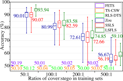
Figure 1: Detection performances of existing LS methods in datasets with various ratios. The box plot depicts the overall performance of these methods on 10 user datasets, as introduced in Section 3.1. In each box, the solid circles represent extreme value in 10 performances, while the hollow squares represent average value in 10 performances, as marked by the labels.

The results in Figure 1 show that the performance of the existing methods is insufficient, and the performance decreases notably with an increasing ratio. This phenomenon is because social network posts exhibit unique user characteristics influenced by various user attributes, resulting in strong personalization. These user characteristics are difficult to imitate in stegos. However, existing LS methods ignore users’ personalized characteristics, resulting in limited effective detection in social networks. Moreover, compared to the vast quantity of covers in social networks, the quantity of stegos is exceedingly small, which poses a substantial challenge for detection.

In this work, we propose the UP4LS, which enhances the performance of existing methods in LS tasks. UP4LS leverages the potential user attributes reflected in post content, thereby creating user profiles and extracting user features. At the same time, BERT is employed to extract content features. Then the content features are guided and learned by user features, and the two types of features are concatenated, further improving feature representation. UP4LS increases sensitivity to stegos during training, enabling the model to capture the distribution of a few stegos more effectively. To facilitate the transplantation of existing methods, the deep-learning feature extraction modules in these methods are retained. The remaining components can be modified according to UP4LS. UP4LS not only improves the performances of prevailing LS methods, but also offers a platform for related-task methods on the LS tasks.

Our main contributions are outlined below.

• To our knowledge, UP4LS is the first work on LS tasks using user profiles. We develop user profiles tailored for LS by analyzing user attributes like habits, psychology, and focus within post content. Specific feature extraction modules are designed for the user profile to extract user features, and we explain these features’ rationality and effectiveness for LS.

• To improve feature representation, we employ the attention mechanism to guide the learning of content features by leveraging user features. Then the learning features are concatenated with content features to obtain the final steganalysis features for LS.

• To evaluate UP4LS’s performance, we collected posts from multiple users and curated datasets with various degrees of imbalance (ratios). Experiments show that UP4LS not only improves the performances of existing LS methods in social networks but also opens new avenues for related research on LS tasks.

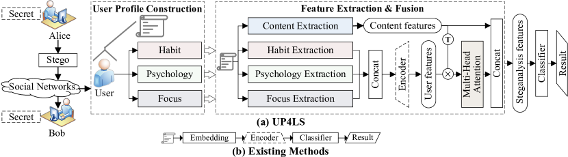
Figure 2: The overall architecture of UP4LS. UP4LS architecture mainly consists of two modules: "User Profile Construction" and "Feature Extraction & Fusion". "(b) Existing Methods" provides the overall architecture of existing methods. UP4LS takes in texts as input, a mixture of covers and stegos. The output is the judgment results of these texts. Initially, the user profile for LS is constructed based on potential user attributes reflected in their posts. This user profile is divided into three types of user attributes: "Habit", "Psychology", and "Focus". Subsequently, corresponding features are extracted based on these user attributes. The deep-learning extraction (called "Encoder") in existing methods is used to map these features to high-dimensional user features. On this basis, these user and content features are fused by mutual attention, and "Classifier" is employed for detection. To enhance the performance of existing methods, these methods only need to retain the "Encoder" component, and the rest is modified according to UP4LS.

2 Methodology

2.1 UP4LS Overall

Almost all existing LS methods are primarily focused on capturing statistical differences in content like semantics and grammar Yang et al. (2020)Xu et al. (2022)Wang et al. (2023c)Peng et al. (2023). However, these methods usually overlook the subjective aspects of human expression in writing. As a result, their effectiveness tends to be suboptimal when applied to social networks. Indeed, users on social networks often reveal potential attributes in their posts. UP4LS examines deeply these user attributes. The user profile for LS is constructed and the user features are obtained. Figure 2 illustrates the overall architecture of UP4LS.

2.2 User Profile Construction

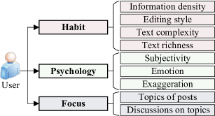
Figure 3: The specific user profile constructed by three user attributes for LS.

User Profile for LS.

From a macro perspective, the construction of the general user profile can effectively improve decision-making effects by analyzing user characteristics and behaviors Mehta et al. (2022)Cai et al. (2023). Currently, there are no steganography schemes that can combine content and user behavior Li et al. (2022) for information hiding. Therefore, we focus on the content of user posts itself. We aim to build a user profile reflecting habits, psychology, and focus. Figure 3 illustrates the specific user profile for LS.

Habit.

It involves the "information density", "editing style", "text richness", and "text complexity" of the posts. Each user exhibits a unique writing style within their posts. This uniqueness often stems from the user’s growth background, cultural upbringing, and life experience. For instance, highly educated users may exhibit more rigorous and professional expressions; while those from specific cultural environments may frequently employ vocabulary and rhetorical techniques unique to their culture. Each user’s distinctive upbringing adds personalization to their expression.

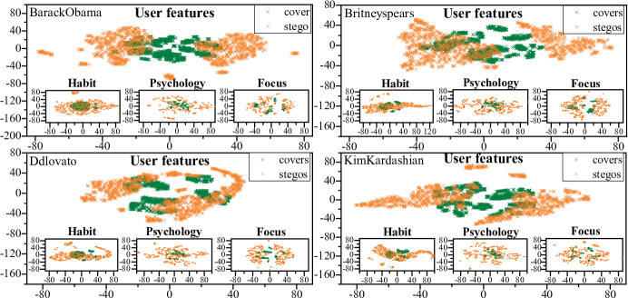
Figure 4: Distribution of covers and stegos in user feature space. Taking 4 users as examples, their usernames are presented in the upper left corner of each subfigure. For more details about the user datasets, please see Section 3.1. We use t-distributed Stochastic Neighbor Embedding (t-SNE) L (2014) to reduce the dimensionality and visualize the user features of texts. The green and orange marks represent the user feature distribution of covers and stegos. Each subfigure contains three small figures, which are the feature distribution of "Habit", "Psychology", and "Focus" attributes. It is worth noting that the user features in this figure are not backpropagated and optimized, they are directly extracted in one go. This figure serves to show the rationality and effectiveness of user features for LS tasks in social networks.

Psychology.

It involves the "subjectivity", "emotion", and "exaggeration" reflected in the posts. Subjectivity in a post can reveal a user’s opinion tendencies. Some users may display strong subjectivity when expressing their opinions, while some users may prioritize objective facts. Emotional elements contained in posts can provide insights into the user’s emotional state. The degree of exaggeration embodied in a post can reveal a user’s specific style. Analyzing these psychological attributes helps obtain personalized characteristics like a user’s personality type and both long and short-term emotional dispositions.

Focus.

It involves the "topics of posts" and "discussions on topics". Users’ areas of focus often reflect their knowledge and interests. This selective focus can indicate their social role, professional background, or current life stage.

In the subsequent sections, we will design specific feature extraction modules for these user attributes. These modules will play an important role in LS tasks in social networks.

2.3 Feature Extraction & Fusion

User Features.

Current steganography struggles to imitate user personalization characteristics during embedding, which results in differences between covers and stegos in this dimension. Capturing these differences and extracting such features can improve LS performance in social networks.

To better capture these differences, we designed a feature extraction module for each user attribute within the user profile. These modules include "Habit Extraction", "Psychology Extraction", and "Focus Extraction". Figure 4 illustrates the distribution of covers and stegos in user feature space. We can get from Figure 4 that user features are reasonable and effective for LS tasks.

Habit Extraction.

This is the first module for these extraction modules. It aims to capture various aspects of writing habits, encompassing factors like "Information density", "Editing style", "Text richness", and "Text complexity". Users usually reflect their underlying writing habits when editing posts, and it is difficult for existing steganography to completely imitate these habits.

"Information density" is captured by analyzing the scale and distribution of nouns, pronouns, and verbs within the text.

"Editing style" is determined by examining the scale and distribution of function words Yoshimi et al. (2023)Liang et al. (2023)Rönnqvist et al. (2022), such as prepositions, determiners, and coordinating conjunctions. Prior research in other fields has shown the feasibility of distinguishing individual editing styles by analyzing function words.

"Text richness" is evaluated by capturing the scale and distribution of adjectives and adverbs. To perform this analysis, we use Python’s NLTK library for part-of-speech tagging, enabling us to count the scale and distribution of various words based on the tagging results. For more detailed information about part-of-speech tag categories, please refer to the Learntek documentation.

"Text complexity" is quantified by calculating sentence length, word length, and scale and distribution of symbols. Typically, spoken texts exhibit simplified grammar, shorter sentences, and shorter word lengths. Increased usage of punctuation marks within a sentence indicates more pauses, leading to a higher degree of fragmentation and a stronger oral language nature. Conversely, a more pronounced written style features a reduced frequency of punctuation marks, there is ${f_{frag}}={1\mathord{\left/{\vphantom{1{count(\mathrm{punc})}}}\right.\kern-1.2pt}{count(\mathrm{punc})}},\mathrm{punc}=\{,.;?!\cdots\}$ . Figure 5 illustrates the working principle of the "Habit Extraction" module.

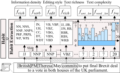
Figure 5: The working principle of the "Habit Extraction" module. The input of this module is text, and the output is extracted features about the dimension of "Information density", "Editing style", "Text richness", and "Text complexity".

Psychology Extraction.

It is the second module for these extraction modules. To analyze "Subjectivity" and "Emotion", we employ Python’s TextBlob library. This library provides a set of APIs that simplify common text analysis tasks. In recent years, TextBlob has gained significant attention for its outstanding performance in sentiment analysis Mirzaei et al. (2023)Otieno et al. (2023). During emotional calculations, TextBlob uses a dictionary that encompasses parameters like "polarity", "subjectivity", and "intensity". This dictionary identifies words, phrases, and symbols in texts related to emotional polarity and subjectivity. Given a text input, it returns a named tuple representing sentiment and subjectivity as "(polarity, subjectivity)". The formulas of the "Emotion" and "Subjectivity" functions are shown below.

$$\mathrm{Emotion}=\frac{{\sum\limits_{i=0}^{K}{{{(-0.5)}^{n}}\times{S_{i\_adverb}}\times{S_{punc}}}}}{{K/{S_{emoticon}}}},$$ (1)

$${S_{i\_adverb}}={\mathrm{max}}(-1,\mathrm{min}({S_{i}}\times{S_{adverb}},1)),$$ (2)

$$\mathrm{Subjectivity}={\mathrm{max(0}},\mathrm{min}(\sum\limits_{i=0}^{K}{S{{}^{\prime}_{i}}\times S{{}^{\prime}_{adverb}}},1)),$$ (3)

where, $K$ is the number of words related to emotional polarity and subjectivity in the text. ${S_{i\_adverb}},{S_{punc}},$ and ${S_{emoticon}}$ represent the emotional value of adverbs, punctuation, and expressions of various degrees. $S{{}^{\prime}_{i}}$ and $S{{}^{\prime}_{adverb}}$ represent the subjective value of the current emotional word and emotional adverb. $n$ represents the number of negative words related to the current emotional vocabulary. The model captures "Exaggeration" by analyzing the frequency of interjections.

Consider that users may have different habits when expressing emotions, resulting in varying degrees of exaggeration in text. The use of interjections is a significant feature Dingemanse and Liesenfeld (2022)Cathcart et al. (2003). In this paper, we define interjections as words that are longer than four letters but have fewer than half the number of unique letters in total length. The formula for identifying interjections is shown below.

$${f_{exag}}=\left\{{\begin{array}[]{*{20}{c}}{0,{\mathrm{}}else}\\ {\frac{1}{{c({t_{i}})}},{\mathrm{}}len({t_{i}})>4\&c(t_{i}^{r})\geq\frac{len({t_{i}})}{2}}\end{array}}\right.,$$ (4)

where, $c(\cdot)$ is the count, and $t_{i}^{r}$ is the repeated character ${t_{i}}$.

Focus Extraction.

It is the last module for these extraction modules. We employ Latent Dirichlet Allocation (LDA) to analyze the "Topics of posts". LDA is an unsupervised clustering algorithm based on Bayesian principles Zhang et al. (2022). Given a collection of document $\mathbb{D}=\{{D_{1}},{D_{2}},\cdots,{D_{j}}\}$ and a predefined number of topics, denoted as $k$, LDA iteratively traverses the corpus and uses Gibbs sampling to update the assigned topic of each word. The algorithm ultimately generates a topic-word co-occurrence frequency matrix. The process outputs the Dirichlet distribution of each document ${D_{j}}$ on potential topics, that is, a probability distribution ${p_{j}}$ on all topics.

In social networks, users often include hyperlinks when commenting on or sharing hot topics. These hyperlinks, typically consist of irregular characters strings, are unlikely to be present in or even considered part of the alternative vocabulary list. Furthermore, since stego is generated based on a candidate word list, the probability of a hyperlink string appearing within it is very low. Therefore, we employ the presence of hyperlinks as a direct criterion to analyze "Discussions on topics".

Encoder.

These three types of features are then concatenated, and the "Encoder", the deep-learning network, maps these features to high-dimensional user features. For existing methods in LS and related tasks, the "Encoder", is the deep-learning module such as LSTM Zou et al. (2021), CNN Xu et al. (2022), and fully connected layer Wang et al. (2023a). This is the focus of the model design and the main source of method advantages. The "Encoder" of these methods is described in the corresponding references. Therefore, to enhance the performance of these methods in social networks, the "Encoder" in these methods is retained, and the rest can be modified according to UP4LS.

Content Features.

In previous studies on LS tasks, researchers used language embedding techniques, such as Word2Vec Mikolov et al. (2013), GloVe Pennington et al. (2014), and BERT Devlin et al. (2018), to extract semantic features. Then, models like LSTM Zou et al. (2021) and CNN Xu et al. (2022) have been used to capture various features. These features are mainly at the content level. Given that BERT offers better semantic representation and better comprehension of text context, we employ BERT to extract content features from the text. The text ${t_{i}}$ undergoes character, position, and segment encodings. These encodings are added to obtain ${{\mathbf{E}}^{0}}$. Then, ${{\mathbf{E}}^{0}}$ is fed into an $L$-layer Transformer Vaswani et al. (2017). The content features ${F_{content}}$ are got. The formula is shown below.

$${F_{content}}={{\mathbf{E}}^{L}}=Tr{m_{enc}}({{\mathbf{E}}^{L-1}}),$$ (5)

Feature Fusion.

Since user features ${F_{user}}$ and ${F_{content}}$ are not the same dimension, direct concatenating may result in insufficient performance. To organically combine these features and provide a richer representation, we utilize a multi-head mutual attention to interact with them. The attention matrix $Attn$ is obtained. UP4LS then concatenates $Attn$ and ${F_{content}}$ to get the final steganalysis features $F$. The formulas are shown below.

$$F={\text{Concat}}(Attn,{F_{content}}),$$ (6)

$$Attn=\frac{{Q\times{K^{\text{T}}}}}{{\sqrt{{d_{k}}}}}=\frac{{{F_{user}}\times{F_{content}}^{\text{T}}}}{{\sqrt{{d_{{F_{content}}}}}}},$$ (7)

where, ${d_{{F_{content}}}}$ is the dimension of ${F_{content}}$ and T is the transpose operation.

2.4 Classifier & Training

UP4LS uses a Softmax classifier to transform $F$ into a probability vector to determine whether the given texts are stegos. During the training phase, UP4LS prioritizes the distributions of stegos and optimizes loss calculation with weighting adjustments Lin et al. (2017). The formulas of the loss functions are shown below.

$$loss({p_{t}})=-{\alpha_{t}}{(1-{p_{t}})^{\gamma}}\log({p_{t}}),$$ (8)

$${p_{t}}=\left\{{\begin{array}[]{*{20}{c}}{p,{\text{ }}y=1}\\ {1-p,{\text{ }}y=0}\end{array}}\right.,$$ (9)

where, $\gamma$ is the adjustment factor, $y$ is the label of the actual sample, $p$ is the probability, and ${\alpha_{t}}$ is the weight of the stego loss function.

3 Experiments

In this section, we present the UP4LS’ performance. To ensure fairness and reliability in comparisons between methods, each experiment was repeated five times for every dataset, and the results were averaged to provide the evaluation. Experiments are run on the NVIDIA GeForce RTX 3090 GPU.

3.1 Settings

Dataset.

We novelly constructed four datasets with various ratios of cover:stego. The ratios are 50:1, 100:1, 200:1, and 500:1 in the training sets. The lower rounding way was adopted. The ratio is 1:1 in all testing sets, the training and testing sets are independent of each other.

In each dataset, covers come from posts by 10 Twitter users, the posts of each user are independent of each other. Stegos are generated by the high-performance linguistic steganography ADG Zhang et al. (2021), which first trains a language model based on the posts of each user, and then the stegos are generated by this model and algorithm. ADG employs an adaptive dynamic grouping strategy, and its security has been rigorously analyzed through mathematical methods and practice. In each ratio, every method is performed in these 10 datasets, and the 10 performances are got. Table 1 shows the specific information of the dataset.

Table 1: The specific information of the datasets.

No.	Name	Num of covers		Payload of stegos
		training	testing
U1	ArianaGrande	2,325	580	3.88
U2	BarackObama	2,291	572	4.20
U3	BritneySpears	2,194	548	5.06
U4	Cristiano	1,940	485	4.54
U5	Ddlovato	1,703	425	4.78
U6	JimmyFallon	2,455	613	3.91
U7	Justinbieber	1,660	414	4.12
U8	KimKardashian	2,351	587	4.85
U9	Ladygaga	1,840	459	5.18
U10	Selenagomez	2,243	560	4.39

Baselines.

The comparison consists of two parts. The first part aims to enhance the performance of prevailing LS-task methods. The second part aims to explore innovative related-task methods and explore their effectiveness in LS tasks.

The LS-task baselines include:

non-BERT-based: 1. FETS Yang et al. (2019b), which has shown superior performance compared to manual constructive methods, and 2. TS_RNN Yang et al. (2019c), which exhibits excellent performance on multiple ideal datasets.

BERT-based: 3. Zou Zou et al. (2021), which achieved state-of-the-art performance at that time, 4. SSLS Xu et al. (2022), which displays remarkable performance on mixed sample sets, and 5. LSFLS Wang et al. (2023a), which achieves high performance in the few-shot ideal data.

The related-task baselines include:

Fine-grained emotion classification tasks: 6. HypEmo Chen et al. (2023), which employs hyperbolic space to capture hierarchical structures. It performs best when the label structure is complex or the relationship between classes is ambiguous.

Hierarchical text classification tasks: 7. HiTIN Zhu et al. (2023), which uses a tree isomorphism network to encode the label hierarchy. It performs well in large-scale hierarchical classification tasks.

These methods cover a relatively comprehensive "Encoder" architecture. Given these methods’ widely recognized performance on specific tasks, they are selected as baselines for experiments.

Hyperparameters.

UP4LS uses the "Bert-base-cased" model, consisting of 12 layers and 768-dimensional hidden layer units. The attention incorporates 4 heads with dimensions of 128. ${\gamma}$ is 5, the topic number of the LDA is 2. The detailed hyperparameter settings of the "Encoder" components can be found in the corresponding baseline papers. Adam optimizer Kingma and Ba (2014) is employed with an initial learning rate of 5e-5.

Evaluation metrics.

We use accuracy (Acc) and the F1 score to evaluate the models’ performance. These formulas are shown below.

$$\begin{gathered}{\text{Acc}}=\frac{{{\text{TP + TN}}}}{{{\text{TP + FP + TN + FN}}}},\\ {\text{F1}}={{2\times({\text{P}}\times{\text{R}})}\mathord{\left/{\vphantom{{2\times({\text{P}}\times{\text{R}})}{({\text{P}}+}}}\right.\kern-1.2pt}{({\text{P}}+}}{\text{R}}),\\ \end{gathered}$$ (10)

where, TP, FP, TN, and FN are the quantity of true positive examples, false positive examples, true negative examples, and false negative examples. P and R are the precision and recall.

3.2 Comparison experiments

3.2.1 LS-task baselines

Figure 6 shows the comparison between the LS-task baselines and the corresponding baseline using UP4LS. The overall improvement degree by UP4LS is shown in Table 2.

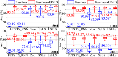
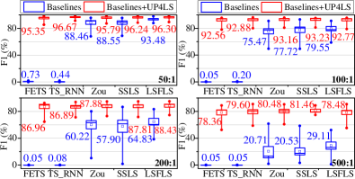
Figure 6: Acc and F1 comparison between the LS-task baselines and the corresponding baseline using UP4LS. The vertical axis on the top half is Acc, and the vertical axis on the bottom half is F1. The horizontal axis is the baselines’ name. The ratios are shown in the lower right corner of each subfigure. The blue box represents the overall performance of the baselines on the 10 user datasets, and the red box represents the overall performance of the corresponding baselines using UP4LS on these datasets. In each box, the solid circle represents the extreme value among the 10 performances, and the hollow square represents the average value among the 10 performances, with specific values numbers. The complete data are shown in Table 5 to Table 9 in Appendix A.

Table 2: Acc and F1 improvement degree of the LS-task baselines by UP4LS in the 10 user datasets. The complete data are shown in Table 5 to Table 9 of Appendix A. For example, when the ratio is 50:1, UP4LS improves the average Acc performance of FETS by 45.40%, which is 95.59%-50.19%=45.40% in Figure 6.

$\Delta$ (Baselines+UP4LS – Baselines)		FETS	TS_RNN	Zou	SSLS	LSFLS	Avg ($\Delta$ of Baselines)
50:1	Acc	45.40	46.65	5.94	6.30	2.49	21.36
	F1	94.62	96.23	7.33	7.69	2.82	41.74
100:1	Acc	43.07	43.25	12.92	11.02	9.70	23.99
	F1	92.51	92.68	17.69	15.51	13.22	46.32
200:1	Acc	38.80	38.64	16.83	16.60	15.06	25.19
	F1	86.91	86.81	27.66	29.91	23.60	50.98
500:1	Acc	32.74	33.26	27.26	28.03	23.68	28.99
	F1	78.31	79.55	59.77	60.93	49.37	65.59
Avg ($\Delta$ of Ratios)	Acc	40.00	40.45	15.74	15.49	12.73	24.88
	F1	88.09	88.82	28.11	28.51	22.25	51.16

The results of Figure 6, Table 2, and the related tables in Appendix A show that: UP4LS can significantly improve the performance of the LS-task baselines in each ratio of user datasets. The overall improvement in Acc and F1 performance reached 24.88% and 51.16%. In the datasets with extremely large ratios, the overall improvement is the most, with Acc improving by 28.99% and F1 improving by 65.59%. In the U1 and U4 user datasets, the overall improvement is the most, with Acc improving by 27.28% and 27.68%.

The reason for the improvement is that UP4LS captures user features by the user profile. Meanwhile, UP4LS can effectively capture stego distributions in the datasets with large ratios, and R can be increased so that F1 is greatly improved.

3.2.2 Related-task baselines

Figure 7 shows the comparison between the related-task baselines and the corresponding baseline using UP4LS. The overall improvement by UP4LS is shown in Table 3.

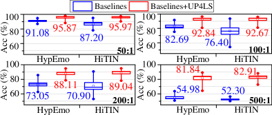
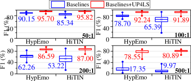
Figure 7: Acc and F1 comparison between the related-task baselines and the corresponding baseline using UP4LS. The meanings of every part in this figure are the same as those in Figure 6. The complete data are shown in Table 10 and Table 11 in Appendix A.

Table 3: Acc and F1 improvement degree of the related-task baselines’ performances by UP4LS in various user datasets at different ratios. The complete data are shown in Table 10 to Table 11 in Appendix A.

$\Delta$ (Baselines+UP4LS – Baselines)		HypEmo	HiTIN	Avg ($\Delta$ of Baselines)
50:1	Acc	4.79	8.77	6.78
	F1	5.55	10.48	8.02
100:1	Acc	10.15	16.27	13.21
	F1	13.54	26.50	20.02
200:1	Acc	15.06	18.14	16.60
	F1	24.33	33.78	29.06
500:1	Acc	26.86	30.61	28.74
	F1	61.20	70.92	66.06
Avg ($\Delta$ of Ratios)	Acc	14.22	18.45	16.34
	F1	26.16	35.42	30.79

The results of Figure 7, Table 3, and the related tables in Appendix A show that: UP4LS can significantly improve the performance of the related-task baselines in each ratio of user datasets.

3.3 Ablation experiment

To verify the effectiveness of user features, the ablation experiment compares the performance of content features (BERT only) with that of user and content features (that is UP4LS). The average performance of 5 LS baselines+UP4LS is used as the performance of user and content features. Figure 8 illustrates the results of the ablation experiment.

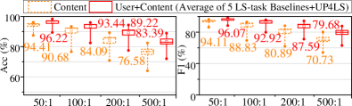
Figure 8: Acc and F1 comparison without and with user features. The horizontal axis represents the ratios, and the vertical axis represents Acc or F1. The orange box represents the overall performance using only content features. The red box represents the overall performance using user and content features. The complete data are shown in Table 12 in Appendix A.

The results of Figure 8 and the related tables in Appendix A show that: User features can improve the performance of baselines. As the ratio increases, the degree of improvement shows an increasing trend. This is attributed to user features reflecting the user’s style to a certain extent. Even with a small quantity of stegos, more comprehensive user features can be captured. Therefore, combining user and content features has a stable performance than using only content features.

3.4 Experiments with sufficient stegos

In addition, we also discussed the scenario with sufficient stegos, and there are 1,500 stegos in each dataset. Table 4 shows the Acc comparison of LS-task baselines and corresponding methods using UP4LS in 10 user datasets with sufficient stegos.

Table 4: Acc comparison of LS-task baselines and corresponding methods using UP4LS in datasets with sufficient stegos. Bold values represent the best Acc. The complete data are shown in Table 13 in Appendix A.

1,500 stegos	Avg (10 Users)
	Baselines	Baselines+UP4LS
FETS	74.95	99.08
TS_RNN	93.93	99.10
Zou	98.67	99.09
SSLS	98.69	99.10
LSFLS	99.00	99.17

The results of Table 4 show that: when the stegos are sufficient, UP4LS can still improve the performance of baselines to a high level. The average performance exceeds 99.00% for every baseline.

4 Conclusion

In this paper, we propose UP4LS, which leverages the user profile for enhancing LS. Through an in-depth analysis of the posts’ content, we have explored three types of user attributes. UP4LS extracts user features by the designed extraction modules. Experiments show that UP4LS can significantly enhance LS performance in social networks. Related-task methods can perform their effect by using UP4LS on LS tasks. To ensure the extraction-targeted user features, we specifically extracted these features and mapped them to high-dimensional space using deep-learning models.

Future research will design a steganography scheme that combines user behavior and content. LS methods can then be developed that leverage user behavior. It extracts features more comprehensively and detects covert communications more directly. Meanwhile, with the development of large models such as GPT4 and LLaMA, we will design large-model watermarking and LS methods based on user characteristics to protect personal privacy. In addition, stegos in social networks may be generated and mixed by multiple steganography schemes. There is little research on the detection of this type of stegos. Therefore, we will also delve into the research of these works next.

Limitations

This paper constructs the user profile and extracts user features that are beneficial to detect stegos. While this research improves the performance of existing methods, it still faces certain limitations: (1) User profile completeness: Although we strive to comprehensively analyze user attributes, the given user profile may not encompass all aspects like user metadata. Moreover, exploring extraction from other user behaviors could potentially uncover additional attributes beneficial to LS. (2) The broad advantage in ideal data: In ideal data, UP4LS may not be able to improve the baselines’ performance. There are slight or even no user attributes reflected in these data. User features hardly improve the performance in these data.

Appendix A Appendix A

Table 5: The detection performance of FETS baseline with and without UP4LS in different datasets. Bold values are the degree of improvement of the baseline after using UP4LS. Red values are the average performance improvement of UP4LS for this baseline in different user datasets with different ratios.

FETS			U1	U2	U3	U4	U5	U6	U7	U8	U9	U10	Avg (10 Users)
50:1	Baseline	Acc	50.09	50.00	50.27	50.52	50.47	50.00	50.24	50.26	50.00	50.00	50.19
		F1	0.34	0.00	1.09	2.04	1.86	0.00	0.96	1.02	0.00	0.00	0.73
	Baseline+UP4LS	Acc	95.09	95.98	96.26	96.91	96.24	98.12	87.20	95.06	97.28	97.77	95.59
		F1	95.12	95.86	96.14	96.96	96.09	98.14	85.40	94.81	97.29	97.72	95.35
	$\Delta$	Acc	45.00	45.98	45.99	46.39	45.77	48.12	36.96	44.80	47.28	47.77	45.40
		F1	94.78	95.86	95.05	94.92	94.23	98.14	84.44	93.79	97.29	97.72	94.62
100:1	Baseline	Acc	50.00	50.00	50.00	50.00	50.00	50.00	50.12	50.00	50.00	50.00	50.01
		F1	0.00	0.00	0.00	0.00	0.00	0.00	0.48	0.00	0.00	0.00	0.05
	Baseline+UP4LS	Acc	94.19	95.80	94.01	94.62	93.79	95.02	81.16	93.10	94.34	94.77	93.08
		F1	94.19	95.62	93.56	94.29	93.36	94.77	77.90	93.40	94.00	94.49	92.56
	$\Delta$	Acc	44.19	45.80	44.01	44.62	43.79	45.02	31.04	43.10	44.34	44.77	43.07
		F1	94.19	95.62	93.56	94.29	93.36	94.77	77.42	93.40	94.00	94.49	92.51
200:1	Baseline	Acc	50.00	50.00	50.00	50.00	50.00	50.00	50.12	50.00	50.00	50.00	50.01
		F1	0.00	0.00	0.00	0.00	0.00	0.00	0.48	0.00	0.00	0.00	0.05
	Baseline+UP4LS	Acc	83.88	92.22	92.96	88.87	91.29	91.19	75.02	92.25	88.89	91.52	88.81
		F1	81.58	92.21	92.49	87.59	90.80	90.36	64.69	91.66	87.50	90.73	86.96
	$\Delta$	Acc	33.88	42.22	42.96	38.87	41.29	41.19	24.90	42.25	38.89	41.52	38.80
		F1	81.58	92.21	92.49	87.59	90.80	90.36	64.21	91.66	87.50	90.73	86.91
500:1	Baseline	Acc	50.00	50.00	50.00	50.00	50.00	50.00	50.12	50.00	50.00	50.00	50.01
		F1	0.00	0.00	0.00	0.00	0.00	0.00	0.48	0.00	0.00	0.00	0.05
	Baseline+UP4LS	Acc	86.72	86.10	84.05	88.76	82.47	80.85	66.43	89.85	74.62	87.68	82.75
		F1	83.42	84.24	81.08	87.74	78.74	74.95	52.56	88.94	65.99	85.98	78.36
	$\Delta$	Acc	36.72	36.10	34.05	38.76	32.47	30.85	16.31	39.85	24.62	37.68	32.74
		F1	83.42	84.24	81.08	87.74	78.74	74.95	52.08	88.94	65.99	85.98	78.31
Avg ($\Delta$ of Ratios)		Acc	39.95	42.53	41.75	42.16	40.83	41.30	27.30	42.50	38.78	42.94	40.00
		F1	88.49	91.98	90.55	91.14	89.28	89.56	69.54	91.95	86.20	92.23	88.09

Table 6: The detection performance of TS_RNN baseline with and without UP4LS in different datasets. The meanings of Bold and Red are the same as those shown in Table 5.

TS_RNN			U1	U2	U3	U4	U5	U6	U7	U8	U9	U10	Avg (10 Users)
50:1	Baseline	Acc	50.00	50.52	50.00	50.1	50.12	50.08	50.00	50.09	50.11	50.09	50.11
		F1	0.00	2.08	0.00	0.41	0.47	0.33	0.00	0.34	0.43	0.36	0.44
	Baseline+UP4LS	Acc	96.90	96.50	97.72	96.70	97.76	98.86	91.67	95.66	97.93	97.86	96.76
		F1	96.90	96.43	97.68	96.60	97.71	98.85	91.28	95.51	97.90	97.81	96.67
	$\Delta$	Acc	46.90	45.98	47.72	46.60	47.64	48.78	41.67	45.57	47.82	47.77	46.65
		F1	96.90	94.35	97.68	96.19	97.24	98.52	91.28	95.17	97.47	97.45	96.23
100:1	Baseline	Acc	50.00	50.17	50.00	50.10	50.00	50.00	50.12	50.00	50.00	50.09	50.05
		F1	0.00	0.70	0.00	0.41	0.00	0.00	0.48	0.00	0.00	0.36	0.20
	Baseline+UP4LS	Acc	93.10	96.24	94.18	95.88	94.71	95.32	82.00	93.78	93.46	94.29	93.30
		F1	92.95	96.20	93.88	95.71	94.41	95.09	80.11	93.42	93.01	93.98	92.88
	$\Delta$	Acc	43.10	46.07	44.18	45.78	44.71	45.32	31.88	43.78	43.46	44.20	43.25
		F1	92.95	95.50	93.88	95.30	94.41	95.09	79.63	93.42	93.01	93.62	92.68
200:1	Baseline	Acc	50.00	50.09	50.00	50.00	50.00	50.00	50.00	50.12	50.00	50.00	50.02
		F1	0.00	0.35	0.00	0.00	0.00	0.00	0.00	0.48	0.00	0.00	0.08
	Baseline+UP4LS	Acc	85.60	94.32	91.51	88.64	88.73	91.27	77.29	90.41	87.69	91.16	88.66
		F1	84.23	94.06	90.75	85.99	86.85	90.69	71.25	88.79	85.96	90.30	86.89
	$\Delta$	Acc	35.60	44.23	41.51	38.64	38.73	41.27	27.29	40.29	37.69	41.16	38.64
		F1	84.23	93.71	90.75	85.99	86.85	90.69	71.25	88.31	85.96	90.30	86.81
500:1	Baseline	Acc	50.00	50.00	50.00	50.00	50.00	50.00	50.00	50.12	50.00	50.00	50.01
		F1	0.00	0.00	0.00	0.00	0.00	0.00	0.00	0.48	0.00	0.00	0.05
	Baseline+UP4LS	Acc	80.26	90.73	84.95	90.10	81.53	82.22	74.40	89.37	74.14	85.00	83.27
		F1	76.70	89.87	82.72	90.98	77.34	78.42	70.80	87.97	58.82	82.39	79.60
	$\Delta$	Acc	30.26	40.73	34.95	40.10	31.53	32.22	24.40	39.25	24.14	35.00	33.26
		F1	76.70	89.87	82.72	90.98	77.34	78.42	70.80	87.49	58.82	82.39	79.55
Avg ($\Delta$ of Ratios)		Acc	38.97	44.25	42.09	42.78	40.65	41.90	31.31	42.22	38.28	42.03	40.45
		F1	87.70	93.88	91.26	92.22	89.08	90.76	78.24	91.18	83.92	91.03	88.82

Table 7: The detection performance of Zou baseline with and without UP4LS in different datasets. The meanings of Bold and Red are the same as those shown in Table 5.

Zou			U1	U2	U3	U4	U5	U6	U7	U8	U9	U10	Avg (10 Users)
50:1	Baseline	Acc	88.02	93.36	85.40	92.06	91.41	93.88	75.72	92.08	92.37	95.80	90.01
		F1	86.47	92.90	82.91	91.38	90.63	93.50	68.04	91.44	91.75	95.62	88.46
	Baseline+UP4LS	Acc	95.74	97.68	95.44	97.01	97.06	98.22	88.41	95.83	97.17	96.96	95.95
		F1	95.76	97.67	95.25	97.03	97.03	98.22	87.20	95.70	97.09	96.90	95.79
	$\Delta$	Acc	7.72	4.32	10.04	4.95	5.65	4.34	12.69	3.75	4.80	1.16	5.94
		F1	9.29	4.77	12.34	5.65	6.40	4.72	19.16	4.26	5.34	1.28	7.33
100:1	Baseline	Acc	75.43	91.70	80.02	78.76	74.35	90.78	66.43	83.05	85.62	83.75	80.99
		F1	67.43	90.94	75.03	73.04	65.51	89.87	49.45	79.59	83.21	80.60	75.47
	Baseline+UP4LS	Acc	93.10	96.50	94.56	95.77	94.82	94.94	83.70	95.40	94.46	95.87	93.91
		F1	92.69	95.39	93.34	95.86	93.58	94.69	80.84	95.34	94.16	95.68	93.16
	$\Delta$	Acc	17.67	4.80	14.54	17.01	20.47	4.16	17.27	12.35	8.84	12.12	12.92
		F1	25.26	4.45	18.31	22.82	28.07	4.82	31.39	15.75	10.95	15.08	17.69
200:1	Baseline	Acc	52.76	75.61	67.34	72.68	71.29	83.44	69.79	73.68	78.00	81.52	72.61
		F1	10.46	67.75	51.49	62.41	59.74	80.20	56.72	64.28	71.79	77.33	60.22
	Baseline+UP4LS	Acc	85.26	94.93	92.24	86.62	91.27	93.36	78.14	90.56	89.54	92.50	89.44
		F1	82.88	94.81	91.61	84.28	90.39	92.49	73.11	89.03	88.32	91.89	87.88
	$\Delta$	Acc	32.50	19.32	24.90	13.94	19.98	9.92	8.35	16.88	11.54	10.98	16.83
		F1	72.42	27.06	40.12	21.87	30.65	12.29	16.39	24.75	16.53	14.56	27.66
500:1	Baseline	Acc	50.69	66.35	51.82	50.52	54.00	72.35	51.09	54.94	50.65	64.29	56.67
		F1	2.72	49.41	7.04	2.04	14.81	61.78	4.26	17.98	2.58	44.44	20.71
	Baseline+UP4LS	Acc	82.50	88.72	83.03	84.35	81.91	80.49	72.28	88.76	86.06	91.16	83.93
		F1	79.31	87.44	80.38	81.45	77.60	75.40	61.02	87.78	83.92	90.53	80.48
	$\Delta$	Acc	31.81	22.37	31.21	33.83	27.91	8.14	21.19	33.82	35.41	26.87	27.26
		F1	76.59	38.03	73.34	79.41	62.79	13.62	56.76	69.80	81.34	46.09	59.77
Avg ($\Delta$ of Ratios)		Acc	22.43	12.70	20.17	17.43	18.50	6.64	14.88	16.70	15.15	12.78	15.74
		F1	45.89	18.58	36.03	32.44	31.98	8.86	30.93	28.64	28.54	19.25	28.11

Table 8: The detection performance of SSLS baseline with and without UP4LS in different datasets. The meanings of Bold and Red are the same as those shown in Table 5.

SSLS			U1	U2	U3	U4	U5	U6	U7	U8	U9	U10	Avg (10 Users)
50:1	Baseline	Acc	90.09	94.93	93.25	87.22	88.94	95.60	76.21	88.50	90.20	95.71	90.07
		F1	89.20	94.68	92.76	85.34	87.63	95.39	68.78	87.08	89.13	95.53	88.55
	Baseline+UP4LS	Acc	95.67	97.53	95.75	97.34	97.76	98.24	89.20	97.00	97.10	98.12	96.37
		F1	95.55	97.50	95.58	97.30	97.73	98.25	88.38	96.99	97.01	98.12	96.24
	$\Delta$	Acc	5.58	2.60	2.50	10.12	8.82	2.64	12.99	8.50	6.90	2.41	6.30
		F1	6.35	2.82	2.82	11.96	10.10	2.86	19.60	9.91	7.88	2.59	7.69
100:1	Baseline	Acc	79.22	91.35	80.66	76.70	87.29	93.56	66.30	75.13	86.71	88.93	82.59
		F1	73.89	90.54	76.02	69.62	85.48	93.15	49.36	66.89	84.67	87.55	77.72
	Baseline+UP4LS	Acc	92.90	95.37	93.70	95.05	94.59	95.11	83.48	95.03	95.53	95.36	93.61
		F1	92.75	95.15	93.88	94.81	94.28	94.86	81.22	94.80	95.34	95.16	93.23
	$\Delta$	Acc	13.68	4.02	13.04	18.35	7.30	1.55	17.18	19.90	8.82	6.43	11.02
		F1	18.86	4.61	17.86	25.19	8.80	1.71	31.86	27.91	10.67	7.61	15.51
200:1	Baseline	Acc	55.69	79.11	64.60	73.09	71.41	88.25	50.48	69.59	87.36	87.05	72.66
		F1	20.68	74.38	45.20	63.19	59.97	86.72	1.91	56.30	85.54	85.13	57.90
	Baseline+UP4LS	Acc	86.03	95.02	92.06	88.37	91.60	92.17	77.85	88.47	89.43	91.61	89.26
		F1	85.69	94.92	91.38	86.54	90.76	91.50	71.74	86.49	88.19	90.84	87.81
	$\Delta$	Acc	30.34	15.91	27.46	15.28	20.19	3.92	27.37	18.88	2.07	4.56	16.60
		F1	65.01	20.54	46.18	23.35	30.79	4.78	69.83	30.19	2.65	5.71	29.91
500:1	Baseline	Acc	50.86	56.91	52.37	55.26	54.71	70.64	53.26	51.62	55.01	61.25	56.19
		F1	3.39	24.27	9.06	19.03	17.20	58.53	12.64	6.27	18.22	36.73	20.53
	Baseline+UP4LS	Acc	81.72	89.51	79.84	89.69	82.24	82.14	78.62	88.33	80.17	89.91	84.22
		F1	79.73	88.39	74.80	88.91	78.52	78.51	74.75	86.91	75.27	88.80	81.46
	$\Delta$	Acc	30.86	32.60	27.47	34.43	27.53	11.50	25.36	36.71	25.16	28.66	28.03
		F1	76.34	64.12	65.74	69.88	61.32	19.98	62.11	80.64	57.05	52.07	60.93
Avg ($\Delta$ of Ratios)		Acc	20.12	13.78	17.62	19.55	15.96	4.90	20.73	21.00	10.74	10.52	15.49
		F1	41.64	23.02	33.15	32.60	27.75	7.33	45.85	37.16	19.56	17.00	28.51

Table 9: The detection performance of LSFLS baseline with and without UP4LS in different datasets. The meanings of Bold and Red are the same as those shown in Table 5.

LSFLS			U1	U2	U3	U4	U5	U6	U7	U8	U9	U10	Avg (10 Users)
50:1	Baseline	Acc	90.28	95.72	93.12	92.27	94.35	97.88	88.89	95.40	95.10	96.34	93.94
		F1	89.18	95.53	92.56	91.68	94.01	97.84	87.80	95.18	94.85	96.21	93.48
	Baseline+UP4LS	Acc	94.40	97.52	97.45	97.22	96.47	98.09	90.34	97.31	97.80	97.70	96.43
		F1	94.22	97.48	97.45	97.17	96.51	98.08	89.36	97.30	97.76	97.68	96.30
	$\Delta$	Acc	4.12	1.80	4.33	4.95	2.12	0.21	1.45	1.91	2.70	1.36	2.49
		F1	5.04	1.95	4.89	5.49	2.50	0.24	1.56	2.12	2.91	1.47	2.82
100:1	Baseline	Acc	79.86	91.78	80.93	82.89	77.65	91.68	70.77	81.09	89.83	89.29	83.58
		F1	74.75	91.05	76.44	79.35	71.30	90.93	58.70	76.68	88.26	88.00	79.55
	Baseline+UP4LS	Acc	92.67	95.72	93.47	94.33	93.51	94.60	81.67	95.40	95.58	95.86	93.28
		F1	92.41	95.59	93.19	93.98	93.02	94.28	78.92	95.22	95.45	95.63	92.77
	$\Delta$	Acc	12.81	3.94	12.54	11.44	15.86	2.92	10.90	14.31	5.75	6.57	9.70
		F1	17.66	4.54	16.75	14.63	21.72	3.35	20.22	18.54	7.19	7.63	13.22
200:1	Baseline	Acc	65.78	82.69	70.44	72.27	70.47	83.03	61.84	71.29	85.73	85.00	74.85
		F1	47.97	79.07	58.03	61.63	58.10	79.57	38.52	59.74	83.35	82.35	64.83
	Baseline+UP4LS	Acc	82.30	95.10	93.70	88.47	92.19	90.98	79.03	93.07	90.85	93.38	89.91
		F1	78.22	95.01	93.92	86.80	91.53	89.00	74.52	92.56	89.93	92.83	88.43
	$\Delta$	Acc	16.52	12.41	23.26	16.20	21.72	7.95	17.19	21.78	5.12	8.38	15.06
		F1	30.25	15.94	35.89	25.17	33.43	9.43	36.00	32.82	6.58	10.48	23.60
500:1	Baseline	Acc	55.00	63.55	59.07	53.51	65.29	64.19	50.36	67.72	55.12	57.14	59.10
		F1	19.69	42.64	27.99	12.40	46.85	44.22	1.44	52.33	18.58	25.00	29.11
	Baseline+UP4LS	Acc	81.21	88.46	84.76	86.08	80.59	76.75	68.12	87.56	83.51	90.71	82.78
		F1	77.62	82.60	82.02	84.39	75.91	69.71	55.41	85.80	80.46	90.85	78.48
	$\Delta$	Acc	26.21	24.91	25.69	32.57	15.30	12.56	17.76	19.84	28.39	33.57	23.68
		F1	57.93	39.96	54.03	71.99	29.06	25.49	53.97	33.47	61.88	65.85	49.37
Avg ($\Delta$ of Ratios)		Acc	14.92	14.92	10.77	16.46	16.29	13.75	5.91	11.83	14.46	10.49	12.73
		F1	27.72	27.72	15.60	27.89	29.32	21.68	9.63	27.94	21.74	19.64	22.25

Table 10: The detection performance of HypEmo baseline with and without UP4LS in different datasets. The meanings of Bold and Red are the same as those shown in Table 5.

HypEmo			U1	U2	U3	U4	U5	U6	U7	U8	U9	U10	Avg (10 Users)
50:1	Baseline	Acc	88.53	94.93	92.70	91.44	89.76	93.23	86.96	91.74	90.41	91.07	91.08
		F1	87.05	94.67	92.13	90.64	88.60	92.74	85.04	90.99	89.40	90.20	90.15
	Baseline+UP4LS	Acc	94.61	96.90	95.67	96.34	97.41	97.96	88.16	96.93	97.17	97.54	95.87
		F1	94.52	96.84	95.53	96.22	97.39	97.92	87.04	96.91	97.10	97.51	95.70
	$\Delta$	Acc	6.08	1.97	2.97	4.90	7.65	4.73	1.20	5.19	6.76	6.47	4.79
		F1	7.47	2.17	3.40	5.58	8.79	5.18	2.00	5.92	7.70	7.31	5.55
100:1	Baseline	Acc	81.55	91.70	79.01	75.26	79.06	90.86	75.48	82.37	88.34	83.30	82.69
		F1	77.38	90.94	73.44	67.12	75.31	89.95	67.52	78.59	86.81	79.96	78.70
	Baseline+UP4LS	Acc	92.23	95.54	91.98	93.99	94.44	94.15	80.80	93.53	96.51	95.25	92.84
		F1	90.54	95.38	91.62	93.54	94.28	93.84	78.66	93.08	96.40	95.05	92.24
	$\Delta$	Acc	10.68	3.84	12.97	18.73	15.38	3.29	5.32	11.16	8.17	11.95	10.15
		F1	13.16	4.44	18.18	26.42	18.97	3.89	11.14	14.49	9.59	15.09	13.54
200:1	Baseline	Acc	74.31	85.75	68.80	68.25	72.71	75.37	62.56	71.64	75.16	75.98	73.05
		F1	65.43	83.38	54.64	53.47	62.46	67.32	40.15	60.40	66.96	68.39	62.26
	Baseline+UP4LS	Acc	82.24	94.84	88.87	86.80	85.32	90.78	78.59	89.95	91.31	92.43	88.11
		F1	78.83	94.74	87.50	84.80	82.43	89.87	76.85	88.85	90.20	91.82	86.59
	$\Delta$	Acc	7.93	9.09	20.07	18.55	12.61	15.41	16.03	18.31	16.15	16.45	15.06
		F1	13.40	11.36	32.86	31.33	19.97	22.55	36.70	28.45	23.24	23.43	24.33
500:1	Baseline	Acc	53.02	63.64	52.28	55.77	58.47	57.34	50.85	53.24	51.74	53.48	54.98
		F1	11.38	42.86	8.73	20.70	28.97	25.60	3.33	12.16	6.74	13.02	17.35
	Baseline+UP4LS	Acc	80.54	88.20	84.43	86.80	80.35	76.00	64.29	85.48	83.01	89.27	81.84
		F1	75.83	87.24	86.78	85.90	80.44	69.37	52.07	83.24	79.90	84.72	78.55
	$\Delta$	Acc	27.52	24.56	32.15	31.03	21.88	18.66	13.44	32.24	31.27	35.79	26.86
		F1	64.45	44.38	78.05	65.20	51.47	43.77	48.74	71.08	73.16	71.70	61.20
Avg ($\Delta$ of Ratios)		Acc	13.05	9.87	17.04	18.30	14.38	10.52	9.00	16.73	15.59	17.67	14.22
		F1	24.62	15.59	33.12	32.13	24.80	18.85	24.65	29.99	28.42	29.38	26.16

Table 11: The detection performance of HiTIN baseline with and without UP4LS in different datasets. The meanings of Bold and Red are the same as those shown in Table 5.

HiTIN			U1	U2	U3	U4	U5	U6	U7	U8	U9	U10	Avg (10 Users)
50:1	Baseline	Acc	79.76	95.11	86.58	83.62	82.59	89.94	78.13	89.69	93.09	93.50	87.20
		F1	74.63	95.00	84.68	81.72	79.94	89.65	73.26	88.39	92.70	93.40	85.34
	Baseline+UP4LS	Acc	93.28	96.68	96.26	96.91	97.27	97.19	90.34	96.95	97.28	97.50	95.97
		F1	92.88	96.60	96.15	96.81	97.20	97.09	89.90	96.89	97.20	97.44	95.82
	$\Delta$	Acc	13.52	1.57	9.68	13.29	14.68	7.25	12.21	7.26	4.19	4.00	8.77
		F1	18.25	1.60	11.47	15.09	17.26	7.44	16.64	8.50	4.50	4.04	10.48
100:1	Baseline	Acc	65.95	93.59	64.94	68.09	87.20	92.41	54.09	87.04	66.35	84.33	76.40
		F1	48.51	92.82	46.28	55.22	88.05	90.78	17.26	84.87	53.93	76.16	65.39
	Baseline+UP4LS	Acc	89.05	95.80	92.43	94.90	94.00	94.72	81.04	93.95	94.77	96.07	92.67
		F1	88.19	95.64	91.81	94.70	93.63	94.35	76.60	93.56	94.48	95.93	91.89
	$\Delta$	Acc	23.10	2.21	27.49	26.81	6.80	2.31	26.95	6.91	28.42	11.74	16.27
		F1	39.68	2.82	45.53	39.48	5.58	3.57	59.34	8.69	40.55	19.77	26.50
200:1	Baseline	Acc	55.14	90.73	63.01	67.51	70.86	85.13	52.93	79.54	53.96	90.14	70.90
		F1	13.80	89.82	43.59	49.14	59.23	86.27	14.38	73.92	13.52	88.50	53.22
	Baseline+UP4LS	Acc	85.02	95.02	90.97	86.29	90.74	92.33	78.09	92.05	88.40	91.52	89.04
		F1	82.33	94.92	90.63	84.33	89.70	91.71	69.82	89.28	86.56	90.75	87.00
	$\Delta$	Acc	29.88	4.29	27.96	18.78	19.88	7.20	25.16	12.51	34.44	1.38	18.14
		F1	68.53	5.10	47.04	35.19	30.47	5.44	55.44	15.36	73.04	2.25	33.78
500:1	Baseline	Acc	51.85	52.45	52.08	51.03	50.06	52.64	52.93	56.33	50.66	52.95	52.30
		F1	7.95	9.33	9.72	4.44	0.94	8.15	9.72	35.41	1.75	12.31	9.97
	Baseline+UP4LS	Acc	81.72	86.88	83.75	84.99	84.21	75.04	72.71	87.95	83.66	88.21	82.91
		F1	79.17	84.18	78.42	82.97	81.04	66.81	76.41	87.12	85.90	86.88	80.89
	$\Delta$	Acc	29.87	34.43	31.67	33.96	34.15	22.40	19.78	31.62	33.00	35.26	30.61
		F1	71.22	74.85	68.70	78.53	80.10	58.66	66.69	51.71	84.15	74.57	70.92
Avg ($\Delta$ of Ratios)		Acc	24.09	10.63	24.20	23.21	18.88	9.79	21.03	14.58	25.01	13.10	18.45
		F1	49.42	21.09	43.19	42.07	33.35	18.78	49.53	21.07	50.56	25.16	35.42

Table 12: Ablation experiment results. Avg (UP4LS) is the average performance of 5 Baselines+UP4LS including the FETS, TS_RNN baselines, and so on. "Content" represents the steganalysis performance that only uses BERT to extract content features. "User+Content" represents the steganalysis performance that uses a combination of user features and content features. The performance of "User+Content" is presented by the average performance of Baselines+UP4LS. $\Delta$ represents the degree of performance improvement brought by user features for steganalysis. Specific values are shown in bold. Bold values are the degree of improvement of the baseline after using UP4LS. Red values are the average performance improvement brought by user characteristics in different user datasets.

Ablation experiment			U1	U2	U3	U4	U5	U6	U7	U8	U9	U10	Avg (10 Users)
50:1	Content	Acc	93.97	95.80	94.71	94.74	95.06	96.08	87.44	94.55	95.97	95.80	94.41
		F1	93.88	95.64	94.41	94.46	94.81	96.05	86.21	94.23	95.80	95.63	94.11
	User+Content	Acc	95.56	97.04	96.52	97.04	97.06	98.31	89.36	96.17	97.46	97.68	96.22
		F1	95.51	96.99	96.42	97.01	97.01	98.31	88.32	96.06	97.41	97.65	96.07
	$\Delta$	Acc	1.59	1.24	1.81	2.30	2.00	2.23	1.92	1.62	1.49	1.88	1.81
		F1	1.63	1.35	2.01	2.55	2.20	2.26	2.11	1.83	1.61	2.02	1.96
100:1	Content	Acc	88.53	93.36	92.43	92.27	91.88	89.89	76.62	91.57	93.25	92.50	90.23
		F1	87.15	92.90	91.81	91.62	91.19	88.75	69.45	90.79	92.76	91.89	88.83
	User+Content	Acc	93.19	95.93	93.98	95.13	94.28	95.00	82.40	94.54	94.67	95.23	93.44
		F1	93.00	95.59	93.57	94.93	93.73	94.74	79.80	94.44	94.39	94.99	92.92
	$\Delta$	Acc	4.66	2.57	1.55	2.86	2.40	5.11	5.78	2.97	1.42	2.73	3.21
		F1	5.85	2.69	1.76	3.31	2.54	5.99	10.35	3.65	1.63	3.10	4.09
200:1	Content	Acc	78.88	89.34	86.51	82.78	86.12	87.19	70.82	85.95	84.42	88.84	84.09
		F1	73.40	88.06	84.28	79.25	83.92	85.31	62.04	83.65	81.55	87.44	80.89
	User+Content	Acc	84.61	94.32	92.49	88.19	91.02	91.79	77.47	90.95	89.28	92.03	89.22
		F1	82.52	94.20	92.03	86.24	90.07	90.81	71.06	89.71	87.98	91.32	87.59
	$\Delta$	Acc	5.73	4.98	5.98	5.41	4.90	4.60	6.65	5.00	4.86	3.19	5.13
		F1	9.12	6.14	7.75	6.99	6.15	5.50	9.02	6.06	6.43	3.88	6.70
500:1	Content	Acc	76.14	81.39	77.55	80.30	74.71	74.05	64.01	81.52	73.64	82.45	76.58
		F1	69.96	80.17	69.32	76.85	66.14	69.27	53.98	77.32	64.20	80.04	70.73
	User+Content	Acc	82.48	88.70	83.33	87.80	81.75	80.49	71.97	88.77	79.70	88.89	83.39
		F1	79.36	86.51	80.20	86.69	77.62	75.40	62.91	87.48	72.89	87.71	79.68
	$\Delta$	Acc	6.34	7.31	5.78	7.50	7.04	6.44	7.96	7.25	6.06	6.44	6.81
		F1	9.40	6.34	10.88	9.84	11.48	6.13	8.93	10.16	8.69	7.67	8.95

Table 13: Comparison of the Acc performance of baselines and corresponding methods using UP4LS in 10 user datasets with sufficient stegos. Bold values represent the best performance.

1,500 stegos		U1	U2	U3	U4	U5	U6	U7	U8	U9	U10	Avg (10 Users)
FETS	Baselines	68.93	77.01	79.26	71.34	75.76	77.89	62.32	79.65	77.56	79.80	74.95
	Baselines+UP4LS	98.77	99.77	98.91	99.18	98.59	99.38	98.70	98.69	99.67	99.18	99.08
TS_RNN	Baselines	94.76	94.13	95.69	87.70	93.76	96.14	94.57	96.24	93.62	92.67	93.93
	Baselines+UP4LS	98.70	99.76	99.09	98.87	98.71	99.47	98.65	98.87	99.78	99.11	99.10
Zou	Baselines	97.87	99.81	98.21	98.97	96.71	99.21	98.55	98.68	99.67	99.05	98.67
	Baselines+UP4LS	98.82	99.77	99.18	98.66	98.94	99.47	98.55	98.78	99.61	99.07	99.09
SSLS	Baselines	98.36	99.62	98.15	98.45	97.24	99.11	98.67	98.57	99.78	98.95	98.69
	Baselines+UP4LS	98.70	99.77	99.09	98.87	98.69	99.38	98.77	98.89	99.72	99.11	99.10
LSFLS	Baselines	98.52	99.74	98.72	98.87	98.59	99.29	98.79	98.61	99.78	99.11	99.00
	Baselines+UP4LS	98.73	99.72	99.09	99.15	99.06	99.56	98.74	98.79	99.69	99.16	99.17

References

- Cai et al. (2023) Pengshan Cai, Kaiqiang Song, Sangwoo Cho, Hongwei Wang, Xiaoyang Wang, Hong Yu, Fei Liu, and Dong Yu. 2023. Generating user-engaging news headlines. In Proceedings of the 61st Annual Meeting of the Association for Computational Linguistics (Volume 1: Long Papers), pages 3265–3280.
- Cathcart et al. (2003) Nicola Cathcart, Jean Carletta, and Ewan Klein. 2003. A shallow model of backchannel continuers in spoken dialogue. In European ACL, pages 51–58.
- Chen et al. (2023) Chihyao Chen, Tunmin Hung, Yili Hsu, and Lunwei Ku. 2023. Label-aware hyperbolic embeddings for fine-grained emotion classification. In Proceedings of the 61st Annual Meeting of the Association for Computational Linguistics (Volume 1: Long Papers), pages 10947–10958.
- Devlin et al. (2018) Jacob Devlin, Ming-Wei Chang, Kenton Lee, and Kristina Toutanova. 2018. Bert: Pre-training of deep bidirectional transformers for language understanding. In arXiv preprint.
- Dingemanse and Liesenfeld (2022) Mark Dingemanse and Andreas Liesenfeld. 2022. From text to talk: Harnessing conversational corpora for humane and diversity-aware language technology. In Proceedings of the 60th Annual Meeting of the Association for Computational Linguistics (Volume 1: Long Papers), pages 5614–5633.
- Kingma and Ba (2014) Diederik P. Kingma and Jimmy Lei Ba. 2014. Adam: A method for stochastic optimization. arXiv preprint.
- L (2014) Van Der Maaten L. 2014. Accelerating t-sne using tree-based algorithms. The journal of machine learning research, 15(1):3221–3245.
- Li et al. (2022) Jian Li, Jieming Zhu, Qiwei Bi, Guohao Cai, Lifeng Shang, Zhenhua Dong, Xin Jiang, and Qun Liu. 2022. Miner: multi-interest matching network for news recommendation. In Findings of the Association for Computational Linguistics: ACL 2022, pages 343–352.
- Liang et al. (2023) Xiaobo Liang, Zecheng Tang, Juntao Li, and Min Zhang. 2023. Open-ended long text generation via masked language modeling. In Proceedings of the 61st Annual Meeting of the Association for Computational Linguistics (Volume 1: Long Papers), pages 223–241.
- Lin et al. (2017) Tsung-Yi Lin, Priya Goyal, Ross Girshick, Kaiming He, and Piotr Dollar. 2017. Focal loss for dense object detection. In Proceedings of the IEEE International Conference on Computer Vision (ICCV), pages 2980–2988.
- Mehta et al. (2022) Nikhil Mehta, Maria Leonor Pacheco, and Dan Goldwasser. 2022. Tackling fake news detection by continually improving social context representations using graph neural networks. In Proceedings of the 60th Annual Meeting of the Association for Computational Linguistics (Volume 1: Long Papers), pages 1363–1380.
- Mikolov et al. (2013) Tomas Mikolov, Kai Chen, Greg Corrado, and Jeffrey Dean. 2013. Efficient estimation of word representations in vector space. arXiv preprint.
- Mirzaei et al. (2023) Maryam Sadat Mirzaei, Kourosh Meshgi, and Satoshi Sekine. 2023. What is the real intention behind this question? dataset collection and intention classification. In Proceedings of the 61st Annual Meeting of the Association for Computational Linguistics (Volume 1: Long Papers), pages 13606–13622.
- Otieno et al. (2023) Denish Omondi Otieno, Akbar Siami Namin, and Keith S. Jones. 2023. The application of the bert transformer model for phishing email classification. In Proceedings of the 2023 IEEE 47th Annual Computers, Software, and Applications Conference (COMPSAC), pages 1303–1310.
- Peng et al. (2023) Wanli Peng, Sheng Li, Zhenxing Qian, and Xinpeng Zhang. 2023. Text steganalysis based on hierarchical supervised learning and dual attention mechanism. IEEE/ACM Transactions on Audio, Speech, and Language Processing, pages 1–14.
- Pennington et al. (2014) Jeffrey Pennington, Richard Socher, and Christopher Manning. 2014. Glove: Global vectors for word representation. In Proceedings of the 2014 Conference on Empirical Methods in Natural Language Processing (EMNLP), pages 1532–1543.
- Rönnqvist et al. (2022) Samuel Rönnqvist, Aki-Juhani Kyröläinen, Amanda Myntti, Filip Ginter, and Veronika Laippala. 2022. Explaining classes through stable word attributions. In Findings of the Association for Computational Linguistics: ACL 2022, pages 1063–1074.
- Taskiran et al. (2006) Cuneyt M. Taskiran, Umut Topkara, Mercan Topkara, and Edward J. Delp. 2006. Attacks on lexical natural language steganography systems. In Proceeding of the Security, Steganography, and Watermarking of Multimedia Contents VIII, volume 6072, pages 97–105.
- Vaswani et al. (2017) Ashish Vaswani, Noam Shazeer, Niki Parmar, Jakob Uszkoreit, Llion Jones, Aidan N. Gomez, Łukasz Kaiser, and Illia Polosukhin. 2017. Attention is all you need. In Proceedings of the 31st Conference on Neural Information Processing Systems (NeurIPS).
- Wang et al. (2023a) Huili Wang, Zhongliang Yang, Jinshuai Yang, Cheng Chen, and Yongfeng Huang. 2023a. Linguistic steganalysis in few-shot scenario. IEEE Transactions on Information Forensics and Security, 18:4870–4882.
- Wang et al. (2023b) Yihao Wang, Ru Zhang, and Jianyi Liu. 2023b. Rls-dts: Reinforcement-learning linguistic steganalysis in distribution-transformed scenario. IEEE Signal Processing Letters, 30:1232–1236.
- Wang et al. (2023c) Yihao Wang, Ru Zhang, and Jianyi Liu. 2023c. V-a3ts: A rapid text steganalysis method based on position information and variable parameter multi-head self-attention controlled by length. Journal of Information Security and Applications, 75:103512.
- Wen et al. (2022) Juan Wen, Ziwei Zhang, Yu Yang, and Yiming Xue. 2022. Few-shot text steganalysis based on attentional meta-learner. In Proceedings of the 2022 ACM Workshop on Information Hiding and Multimedia Security, pages 97–106.
- Xiang et al. (2014) Lingyun Xiang, Xingming Sun, Gang Luo, and Bin Xia. 2014. Linguistic steganalysis using the features derived from synonym frequency. Multimedia Tools and Applications, 71(3):1893–1911.
- Xu et al. (2022) Yimin Xu, Tengyun Zhao, and Ping Zhong. 2022. Small-scale linguistic steganalysis for multi-concealed scenarios. IEEE Signal Processing Letters, 29:130–134.
- Xue et al. (2022a) Yiming Xue, Lingzhi Kong, Wanli Peng, Ping Zhong, and Juan Wen. 2022a. An effective linguistic steganalysis framework based on hierarchical mutual learning. Information Sciences, 586:140–154.
- Xue et al. (2022b) Yiming Xue, Boya Yang, Yaqian Deng, Wanli Peng, and Juan Wen. 2022b. Domain adaptational text steganalysis based on transductive learning. In Proceeding of the ACM Workshop on Information Hiding and Multimedia Security (IH-MMSec), pages 91–96.
- Yang et al. (2022) Jinshuai Yang, Zhongliang Yang, Jiajun Zou, Haoqin Tu, and Yongfeng Huang. 2022. Linguistic steganalysis towards social network. IEEE Transactions on Information Forensics and Security, 18:859–871.
- Yang et al. (2019a) Zhongliang Yang, Xiaoqing Guo, Ziming Chen, Yongfeng Huang, and Yujin Zhang. 2019a. Rnn-stega: Linguistic steganography based on recurrent neural networks. IEEE Transactions on Information Forensics and Security, 14(5):1280–1295.
- Yang et al. (2019b) Zhongliang Yang, Yongfeng Huang, and Yujin Zhang. 2019b. A fast and efficient text steganalysis method. IEEE Signal Processing Letters, 26(4):627–631.
- Yang et al. (2020) Zhongliang Yang, Yongfeng Huang, and Yujin Zhang. 2020. Ts-csw: text steganalysis and hidden capacity estimation based on convolutional sliding windows. Multimedia Tools and Applications, 79:18293–18316.
- Yang et al. (2019c) Zhongliang Yang, Ke Wang, Jian Li, Yongfeng Huang, and Yujin Zhang. 2019c. Ts-rnn: Text steganalysis based on recurrent neural networks. IEEE Signal Processing Letters, 26(12):1743–1747.
- Yoshimi et al. (2023) Nana Yoshimi, Tomoyuki Kajiwara, Satoru Uchida, Yuki Arase, and Takashi Ninomiya. 2023. Distractor generation for fill-in-the-blank exercises by question type. In Proceedings of the 61st Annual Meeting of the Association for Computational Linguistics (Volume 4: Student Research Workshop), pages 276–281.
- Zhang et al. (2022) Linhai Zhang, Xuemeng Hu, Boyu Wang, Deyu Zhou, Qian-Wen Zhang, and Yunbo Cao. 2022. Pre-training and fine-tuning neural topic model: A simple yet effective approach to incorporating external knowledge. In Proceedings of the 60th Annual Meeting of the Association for Computational Linguistics (Volume 1: Long Papers), pages 5980–5989.
- Zhang et al. (2021) Siyu Zhang, Zhongliang Yang, Jinshuai Yang, and Yongfeng Huang. 2021. Provably secure generative linguistic steganography. In Proceeding of the International Joint Conference on Natural Language Processing (ACL-IJCNLP), pages 3046–3055.
- Zhou et al. (2021) Xuejing Zhou, Wanli Peng, Boya Yang, Juan Wen, Yiming Xue, and Ping Zhong. 2021. Linguistic steganography based on adaptive probability distribution. IEEE Transactions on Dependable and Secure Computing, 19(5):2982–2997.
- Zhu et al. (2023) He Zhu, Chong Zhang, Junjie Huang, Junran Wu, and Ke Xu. 2023. Hitin: Hierarchy-aware tree isomorphism network for hierarchical text classification. In Proceedings of the 61st Annual Meeting of the Association for Computational Linguistics (Volume 1: Long Papers), pages 7809–7821.
- Zou et al. (2021) Jiajun Zou, Zhongliang Yang, Siyu Zhang, Sadaqat Rehman, and Yongfeng Huang. 2021. High-performance linguistic steganalysis, capacity estimation and steganographic positioning. In Proceeding of the International Workshop on Digital Watermarking (IWDW), pages 80–93.