Optimal Control with Obstacle Avoidance for Incompressible Ideal Flows of an Inviscid Fluid.

Abstract

It has been shown in [1] that an optimal control formulation for an incompressible ideal fluid flow yields Euler’s fluid equations. In this paper we consider the modified Euler’s equations by adding a potential function playing the role of a barrier function in the corresponding optimal control problem with the motivation of studying obstacle avoidance in the motion of fluid particles for incompressible ideal flows of an inviscid fluid From the physical point of view, imposing an artificial potential in the fluid context is equivalent to generating a desired pressure. Simulation results for the obstacle avoidance task are provided.

I Introduction

It is well known that the flow of Euler equations of a perfect fluid can be interpreted as a geodesic on the group of volume preserving diffeomorphisms of the fluid domain, relative to an $L^{2}$-Riemannian metric [2]. This result has been the origin of many developments in the method of symmetry and reduction for the study of incompressible fluids [3].

Since the seminal work of Arnold [2], the geometric formulation via diffeomorphism group and the associated method of symmetry and reduction has been developed in order to apply the theory to a large class of equations arising in hydrodynamics such as compressible fluids [4] and magnetohydrodynamics in [5].

Optimal control problems for incompressible fluids have been considered in [1], [6], where the authors mainly study the question of whether Euler’s fluid equations represent an optimal control problem and compare the fluid equation arising in an optimal control fashion with the symmetric generalized rigid body equations [7], [8], [9]. In particular, the authors in [1] show that an optimal control approach leads to a standard formulation of the Euler equations – the so-called impulse equations in their Lagrangian form.

In recent years, path planning strategies have become vital in the field of robotics, and more generally, in the field of control engineering. At its core, path planning seeks to construct trajectories that interpolate some set of knot points in an "optimal" way (for example, by minimizing some quantity such as the distance traveled, the time elapsed, or the energy consumed along the path), while completing some additional tasks such as avoiding obstacles in phase space or avoiding inter-agent collisions in the case of multi-agent systems. One of the key cases of path planning arises in rigid body systems. In this case, trajectories can be modelled as paths in $SO(3)\times\mathbb{R}^{3}$ or $\text{SE}(3)$, both of which are Lie groups with physically motivated Riemannian metrics. Finding optimal trajectories can then be interpreted as finding solutions to a variational problem on a Lie group endowed with a Riemannian structure.

Geodesic equations, however, are unable to take the tasks of obstacle avoidance or inter-agent collision avoidance into consideration—which are vital components of path planning in many robotic systems. One strategy, introduced in [10], is to augment the action functional with an artificial potential that grows radially near the obstacles. Necessary conditions for optimality were derived in [10, 11] for the obstacle avoidance task, and in [12, 13] for the collision avoidance task. Reduction by symmetry on Lie groups and on symmetric spaces was considered in [14].

In this paper, we consider the Hamiltonian-Pontryagin variational formulation of the equations of incompressible ideal fluid flow from the point of view of optimal control theory. In particular, with the motivation of controlling the pressure of the fluid, we employ an artificial potential in the cost function and obtain what we call modified Euler’s equations on the Lie group of volume preserving diffeomorphisms. In particular, in Theorem 1 we present necessary conditions for optimal solutions of the variational obstacle avoidance problem for incompressible fluids. These necessary conditions are precisely the Euler-Lagrange equations for the cost functional of an optimal control problem. However, these equations do not explicitly describe the evolution of the velocity field as the Euler equations. So, in Theorem 2 we show that the critical value of the cost functional satisfies the modified Euler equation in terms of the velocity vector field.

The remainder of the paper is structured as follows. In Section II we introduce inviscid, incompressible, fluid flows and the problem formulation for the obstacle avoidance task. Section III contains the main results of the paper about the extremals for the obstacle avoidance optimal control problem and modified Euler’s equations. Finally, in Section IV we show some simulation results. We close the paper with some conclusions and further directions of research. Technical calculations in multi-variable calculus are provided in the Appendix.

II Inviscid, Incompressible, Fluid Flows and problem formulation

II-A Dynamical equations for inviscid incompressible flows

An inviscid fluid flow is a flow of a zero-viscosity fluid. For this class of fluids, the Reynolds number approaches infinity as the viscosity approaches to zero. Moreover, for this class of fluids viscous forces are neglected, and so Navier-Stokes equations reduce to the Euler equations [2].

An incompressible fluid flow is a flow in which the material density is constant, or, equivalently, the divergence of the flow velocity is zero. Incompressible flows do not imply that the fluid itself is incompressible.

The dynamics for inviscid, incompressible fluid flows is given by Euler’s equation for the incompressible flow of an inviscid fluid which are described by the following partial differential equations [2]

$$\frac{\partial v}{\partial t}+v\cdot\hbox{grad}\,v =-\hbox{grad}\,p$$ (1)

$$\hbox{div}\,v =0,\,\ x\in\Omega,\,\ v=v(x,t),\,\,p=p(x,t),$$

where $v$ is the fluid velocity and $p$ is the preassure. Here $\Omega\subset\mathbb{R}^{3}$ denotes the domain. The pressure $p$ is determined by the divergence-free (volume-preserving) constraint $\hbox{div}\,v=0$.

Assumption: We assume from now on that $\Omega$ has a boundary and the tangencial component of $v$ vanishes at the boundary.

Contrary to [1], (see also [15]), we do not assume that the flow is in all the space or in a periodic box with vanishing velocities at infinity. Our assumption is the minimal requirement to satisfy Stokes theorem in the proof of the main result as well as for numerical simulation purposes.

II-B Impulse dynamics

Recall that for a smooth vector field $X$ defined on a domain $U\subset\mathbb{R}^{n}$, its Helmholtz decomposition gives a pair of smooth vector fields $Y,Z\in U\subset\mathbb{R}^{n}$ such that $X(q)=Y(q)+Z(q)$, $Y(q)=-\nabla V(q)$, $\nabla\cdot Z(q)=0$, for $q\in U$, $V\in U\in\mathbb{R}^{n}$ is a smooth scalar potential with gradient $\nabla V$ and $\nabla\cdot Z$ denotes the divergence vector field of $Z$. This decomposition is not unique (see [16] or [17] for instance).

We introduce the impulse density $z$ by its Helmholtz decomposition as

$$z=v+\hbox{grad}\,k,$$ (2)

where $k=k(x,t)$ is an arbitrary scalar field.

By taking the time derivative of (2) we obtain

$$\frac{\partial z}{\partial t}-v\times\hbox{curl}\,z=\hbox{grad}\,\Lambda,\,\,\hbox{div}\,v=0,$$ (3)

where $\displaystyle{\Lambda=\frac{\partial k}{\partial t}-p-\frac{1}{2}v\cdot v}$ is the gauge.

Although any choice of gauge is possible, here we consider the geometric gauge given by $\Lambda=-v\cdot z$. Therefore (3) can be written as

$$\frac{\partial z}{\partial t}+(v\cdot\hbox{ grad})z+(\hbox{grad }v)^{T}z=0,\,\,\hbox{div}\,v=0,$$ (4)

and now the scalar field $k$ is fixed by the equation

$$\frac{dk}{dt}=p-\frac{1}{2}v\cdot v.$$

II-C Coordinate systems for fluid flows

Arnold [2] has shown that Euler equations for an incompressible fluid has a Lagrangian and Hamiltonian description similar to that for the rigid body. For ideal fluids, the configuration space is the Lie group of volume-preserving transformations of the fluid container, a region $\Omega$ in $\mathbb{R}^{2}$ or $\mathbb{R}^{3}$, or a Riemannian manifold in general, possible with boundary, denoted by $\hbox{Diff}_{\hbox{vol}}(\Omega)$, where the group multiplication on the Lie group $\hbox{Diff}_{\hbox{vol}}(\Omega)$ is the composition.

As is explained in [15], one selects $\hbox{Diff}_{\hbox{vol}}(\Omega)$ as the configuration space in a similar fashion as one does for the rigid body dynamics on the special orthogonal group $SO(3)$. Each $\varphi\in\hbox{Diff}_{\hbox{vol}}(\Omega)$ is a map from $\Omega$ to $\Omega$ which takes a reference point $X\in\Omega$ to a current point $x=\varphi(X)\in\Omega$. So, by knowing $\varphi$ we know where each particle of the fluid goes and therefore the current fluid configuration. We assume that $\varphi$ does not have discontinuities, cavitation, and fluid interpenetration. Moreover, we ask that $\varphi$ be volume-preserving to correspond to the assumption of incompressibility.

A motion in an incompressible fluid on a domain $\Omega$ is a family of time-dependent elements of $\hbox{Diff}_{\hbox{vol}}(\Omega)$ which we write as $x=\varphi(X,t)$. The material velocity is defined by $\displaystyle{V(X,t)=\frac{\partial\varphi(X,t)}{\partial t}}$, and the spatial velocity field is given by $v(x,t)=V(X,t)$, where $x$ and $X$ are related by $x=\varphi(X,t)$.

Note that

$$v=\dot{\varphi}\circ\varphi^{-1}$$ (5)

where we supressed $t$ and write $\dot{\varphi}$ for $V$. Note also that (5) gives a map from the space of $(\varphi,\dot{\varphi})$ (material description) to the space of $v$’s (spatial description). In this paper we restrict to the case $\Omega\subset\mathbb{R}^{3}$ with $\varphi$ being a volume-preserving diffeomorphism on $\Omega$, and with Jacobian having unit determinant.

Given a time-dependent smooth function on $\Omega$, also known as, a scalar field, $k:\Omega\times[0,T]\to\mathbb{R}$, we denote the value of its integral over the domain by

$$\langle k\rangle(t)=\int_{\Omega}k(x,t)dx$$

Given two time-dependent vector fields $a,b:\Omega\times[0,T]\to\mathbb{R}^{3}$ consider the inner product

$$\langle a,b\rangle(t)=\int_{\Omega}a^{T}(x,t)b(x,t)dx.$$

Using the diffeomorphism $\varphi$ as a change of variables in the integral and the fact that the Jaconbian of $\varphi$ has unit determinant, we have the identity

$$\langle a\circ\varphi,b\rangle=\langle a,b\circ\varphi^{-1}\rangle.$$ (6)

With this notation, the vorticity of the flow, defined by $\omega:=\text{curl }v$ satisfies the total vorticity equation given by

$$\frac{\partial\varphi}{\partial t}=v\circ\varphi,\,\,\frac{\partial w}{\partial t}=[w,v]:\hbox{div }v=0,$$

where $[\cdot,\cdot]$ denote the Lie bracket of divergence-free smooth vector fields taking values on $\Omega$ which are parallel to the boundary (i.e., the Lie algebra of $\hbox{Diff}_{\hbox{vol}}(\Omega))$.

II-D Problem formulation

Next, we introduce the optimal control problem under study. The problem can be posed as:

$$\min_{v(\cdot)}\int_{0}^{T}\left(\frac{1}{2}\langle v,v\rangle+\int_{\Omega}V\circ\varphi\right)dt$$ (7)

subject to

$$\hbox{div}\,v=0,\quad\frac{\partial\varphi}{\partial t}=v\circ\varphi$$ (8)

and

$$\varphi(X,0)=\varphi_{0}(X),\quad\varphi(X,T)=\varphi_{T}(X)\hbox{ fixed }$$

together with the assumption that $\Omega$ has a boundary $\partial\Omega$ and $v$ vanishes at $\partial\Omega$. Here $V$ denotes a potential function used to avoid certain region in $\Omega$.

The goal is to study this optimal control problem using the Hamilton-Pontryagin formulation.

III Extremals for the obstacle avoidance optimal control problem

To develop Hamilton-Pontryagin method, let us incorporate the constraints (8) in the functional (7) by means of an extended Lagrangian and Lagrange multipliers, in a similar fashion to that of [1] and [6] (see also [18]). Consider the infinite dimensional space of curves:

$$\begin{split}\mathcal{C}=\{(\varphi,&v,\pi,k)\ |\ \varphi:\Omega\times[0,T]\to\Omega,\varphi(\cdot,0)=\varphi_{0},\\ &\varphi(\cdot,T)=\varphi_{T},\varphi(\cdot,t)\in\hbox{Diff}_{\hbox{vol}}(\Omega),\\ &v:\Omega\times[0,T]\to\mathbb{R}^{3},v(\cdot,t)\text{ vanishing at $\partial\Omega$},\\ &\pi:\Omega\times[0,T]\to\mathbb{R}^{3},k:\Omega\times[0,T]\to\mathbb{R}\}\end{split}$$

Consider the action functional $\mathcal{J}:\mathcal{C}\to\mathbb{R}$ defined by

$$\begin{split}\mathcal{J}(\varphi,v,\pi,k)=\int_{0}^{T}&\left[\Big{\langle}\pi,v\circ\varphi-\frac{\partial\varphi}{\partial t}\Big{\rangle}-\frac{1}{2}\langle v,v\rangle\right.\\ &\left.+\langle k\,\text{div}\,v+V\circ\varphi\rangle\right]\end{split}$$

Optimal solutions of the problem in Section II-D must be critical values of the functional $\mathcal{J}$.

Theorem 1.

Critical curves of the functional $\mathcal{J}$ satisfy the necessary conditions for optimality given by the following set of partial differential equations

$$\begin{split}&\frac{\partial\varphi}{\partial t}=v\circ\varphi,\quad\hbox{div }v=0\\ &v=\pi\circ\varphi^{-1}-\hbox{grad }k\\ &\frac{\partial\pi}{\partial t}=-(Tv\circ\varphi)^{T}\pi+\hbox{grad }V\circ\varphi\end{split}$$ (9)

Proof.

Let $(\varphi,v,\pi,k)$ be a critical point of the functional $\mathcal{J}$ and $(\varphi_{s},v_{s},\pi_{s},k_{s})$ be an arbitrary smooth variation of the point $(\varphi,v,\pi,k)$ on $\mathcal{C}$ i.e., it satisfies $(\varphi_{0},v_{0},\pi_{0},k_{0})=(\varphi,v,\pi,k)$. Also denote the derivative of this curve with respect to the parameter $s$ and evauated at $s$ by $(\delta\varphi,\delta v,\delta\pi,\delta k)$. Then

$$\begin{split}0=\delta\mathcal{J}(\varphi,v,&\pi,k)(\delta\varphi,\delta v,\delta\pi,\delta k)=\int_{0}^{T}\Big{\langle}\delta\pi,v\circ\varphi-\frac{\partial\varphi}{\partial t}\Big{\rangle}\\ &+\Big{\langle}\pi,\delta v\circ\varphi+(Tv\circ\varphi)(\delta\varphi)-\frac{\partial\delta\varphi}{\partial t}\Big{\rangle}\\ &-\langle v,\delta v\rangle+\langle\delta k\,\text{div}\,v+k\,\text{div}\,\delta v\rangle\\ &+\langle\text{grad }V\circ\varphi,\delta\varphi\rangle\ dt\end{split}$$

By applying the Fundamental theorem of the calculus of variations (see for instance [19] or [20]), we deduce immediately that

$$\frac{\partial\varphi}{\partial t}=v\circ\varphi,\quad\text{div}v=0$$

Using identity (6), integrating by parts

$$-\int_{0}^{T}\Big{\langle}\pi,\frac{\partial\delta\varphi}{\partial t}\Big{\rangle}=\int_{0}^{T}\Big{\langle}\frac{\partial\pi}{\partial t},\delta\varphi\Big{\rangle}$$

and applying the divergence theorem [17]

$$\begin{split}\int_{\Omega}k(x,t)\,\text{div}\,\delta v(x,t)dx=&-\int_{\Omega}\text{grad }k(x,t)\delta v(x,t)\ dx\\ &+\int_{\partial\Omega}k\,\delta v\cdot n\,dS,\end{split}$$

where the last term vanishes since $v(x,t)$ vanishes on $\partial\Omega$ and we deduce that

$$\begin{split}0=&\int_{0}^{T}\Big{\langle}\pi,\delta v\circ\varphi+(Tv\circ\varphi)(\delta\varphi)-\frac{\partial\delta\varphi}{\partial t}\Big{\rangle}\\ &-\langle v,\delta v\rangle+\langle k\,\text{div}\,\delta v\rangle+\langle\text{grad }V\circ\varphi,\delta\varphi\rangle\ dt\\ =&\int_{0}^{T}\langle\pi\circ\varphi^{-1}-v-\text{grad }k,\delta v\rangle\\ &+\Big{\langle}(Tv\circ\varphi)^{T}\pi+\frac{\partial\pi}{\partial t}+\text{grad }V\circ\varphi,\delta\varphi\Big{\rangle}\ dt\end{split}$$

Thus, again by the fundamental theorem of calculus of variations, we conclude that

$$\begin{split}&v=\pi\circ\varphi^{-1}-\text{grad }k\\ &\frac{\partial\pi}{\partial t}=-(Tv\circ\varphi)^{T}\pi+\text{grad }V\circ\varphi\end{split}$$

∎

The equations (9) appearing in the previous Theorem are precisely the Euler-Lagrange equations for the functional $\mathcal{J}$. However, these equations do not explicitly describe the evolution of the velocity field $v$ as do the Euler equations in (1).

Theorem 2.

If $(\varphi,v,\pi,k)$ is a critical value of the functional $\mathcal{J}$ then $v$ satisfies the modified Euler equation:

$$\begin{split}&\frac{\partial v}{\partial t}+v\cdot\hbox{grad}\,v=-\hbox{grad}\,(p-V)\\ &\hbox{div}\,v=0,\end{split}$$ (10)

Proof.

The second equation is guaranteed by equations (9), so it remains to prove the first. Define the variable $z=\pi\circ\varphi^{-1}=v+\text{grad }k$. Then, differentiating $z$ in time, we get

$$\frac{\partial z}{\partial t}=\frac{\partial\pi}{\partial t}\circ\varphi^{-1}+(T\pi\circ\varphi^{-1})\left(\frac{\partial\varphi^{-1}}{\partial t}\right),$$

and using equations (9) we deduce

$$\begin{split}\frac{\partial z}{\partial t}=&-(Tv)^{T}(\pi\circ\varphi^{-1})+\text{grad }V\\ &+(T\pi\circ\varphi^{-1})\left(\frac{\partial\varphi^{-1}}{\partial t}\right)\\ =&-(Tv)^{T}(z)+\text{grad }V-Tz(v),\\ \end{split}$$

where in the last equality we used the fact that

$$(T\pi\circ\varphi^{-1})\left(\frac{\partial\varphi^{-1}}{\partial t}\right)=-Tz(v)$$

(see Lemma 1 in the Appendix). Therefore, we get the equation

$$\frac{\partial z}{\partial t}+(Tv)^{T}(z)-\text{grad }V+Tz(v)=0.$$

Using the first two items of Lemma 2 in the Appendix we deduce the equation

$$\frac{\partial z}{\partial t}+(z\cdot\text{grad })v+z\times(\text{curl }v)-\text{grad }V+(v\cdot\text{grad })z=0$$

and through the third item of Lemma 2 in the Appendix we simplify the previous equation

$$\frac{\partial z}{\partial t}+\text{grad }(v\cdot z)-v\times(\text{curl }z)-\text{grad }V=0$$

Now, let

$$\Lambda=\frac{\partial k}{\partial t}-p-\frac{1}{2}v\cdot v$$

be a gauge for this field theory. If we impose the gauge choice $\Lambda=-v\cdot z$ we derive an equation describing the same solutions as above given by

$$\frac{\partial z}{\partial t}-v\times(\text{curl }z)-\text{grad }V=\text{grad }\left(\frac{\partial k}{\partial t}-p-\frac{1}{2}v\cdot v\right)$$

Now, observe that as a particular case of item 3 in Lemma 2 we have

$$(v\cdot\text{grad })v=\frac{1}{2}\text{grad }(v\cdot v)-v\times(\text{curl }v).$$

In addition, since $v=z-\text{grad }k$ and $\text{curl (grad }k)=0$, we have

$$v\times(\text{curl }z)=\frac{1}{2}\text{grad }(v\cdot v)-(v\cdot\text{grad })v.$$

Hence,

$$\frac{\partial z}{\partial t}+(v\cdot\text{grad })v-\text{grad }V=\text{grad }\left(\frac{\partial k}{\partial t}-p\right).$$

Finally, replacing $\displaystyle{\frac{\partial z}{\partial t}}$ by $\displaystyle{\frac{\partial v}{\partial t}+\text{grad }\frac{\partial k}{\partial t}}$ we deduce

$$\frac{\partial v}{\partial t}+(v\cdot\text{grad })v=-\text{grad }\left(p-V\right).$$

∎

Remark 1.

The potential function $V$ is an artificial smooth (or at least $C^{2}$) potential function associated with a fictitious force inducing a repulsion from a region $S\subset\Omega$. We consider $S\subset\Omega$ to be the regular zero level set defined by a scalar valued smooth function $f$, for instance, used to describe obstacles as spheres or ellipsoids in the space.

To avoid collision with obstacles we introduce a potential function $V$ defined as the inverse value of the function $f$. The function $V$ goes to infinity near the obstacle and decays to zero at some positive level set far away from the obstacle $S$. This ensures that such an optimal trajectory does not intersect $S$. The use of artificial potential functions to avoid collision was introduced by Khatib (see [21] and references therein) and further studied by Koditschek [22].

Therefore for our obstacle avoidance problems, it is interesting to study solution of equations (10) with an artificial potential of the type

$$V=\frac{\tau}{(x-a)^{2}+(y-b)^{2}+(z-c)^{2}-r^{2}},\quad\tau,r>0$$

for $a,b,c\in\mathbb{R}$.

IV Discretization of modified Euler equations

We integrated the $2$-dimensional version of equation (10) using a finite differences method and we show how the artificial potential can help the fluid avoid a circular obstacle located at a single point, for which no physical barrier exists. It is interesting to note that, from the physical point of view, imposing an artificial potential in the fluid context is equivalent to generating a desired pressure.

First, we used finite differences to approximate the solution of the first equation in (10) using as initial conditions the functions $u(x,y,0)=-\sin y\cos x$ and $v(x,y,0)=\sin y\cos x$. The integration scheme uses an evenly spaced grid to integrate the vector field on the square $[0,4\pi]\times[0,4\pi]/\{0,4\pi\}$ with discrete spacing between squares of $\Delta x=4\pi/30$ and points lying in the border of the square identified. We will denote the grid by $\Delta_{ij}$.

IV-A Discrete operators and Helmholtz projection

To obtain a divergence-free vector field we will use a discretized version of Helmholtz decomposition (see [23, 24, 25]).

Given a vector field in a 2-dimensional grid $\Delta x$-evenly spaced, denoted by $X(i,j)=(u(i,j),v(i,j))$ consider the divergence operator

$$\nabla^{d}\cdot X(i,j)=\frac{u(i+1,j)-u(i-1,j)+v(i,j+1)-v(i,j-1)}{2\Delta x}.$$

Given a scalar field in the same grid, denoted by $\phi(i,j)$ its discrete gradient is defined by

$$\nabla^{d}\phi(i,j)=\left(\frac{\phi(i+1,j)-\phi(i-1,j)}{2\Delta x},\frac{\phi(i,j+1)-\phi(i,j-1)}{2\Delta x}\right)$$

Finally consider the discrete Laplacian of a scalar field defined by

$$\begin{split}&\Delta^{d}\phi(i,j)=\nabla^{d}\cdot\nabla^{d}\phi\\ &=\frac{\phi(i+2,j)+\phi(i-2,j)+\phi(i,j+2)+\phi(i,j-2)-4\phi(i,j)}{4\Delta x^{2}}.\end{split}$$

A discrete divergence free vector field $X_{0}$ is a vector field on the grid satisfying $\nabla^{d}\cdot X_{0}=0$. Given a vector field $X$ on a grid, we can obtain a discrete divergence free vector field called the discrete Helmholtz projection shown in Figure 1 by setting

$$X_{0}=X-\nabla^{d}\phi,$$

where $\phi$ is a scalar field satisfying the discrete Poisson equation:

$$\Delta^{d}\phi=\nabla^{d}\cdot X.$$

With suitable boundary conditions, this scalar field is unique.

IV-B Simulation results

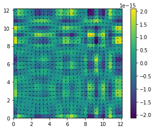
Figure 1: Depiction of the initial conditions. The arrows represent the direction and magnitude of the fluid’s velocity. The color map shows the value of the discrete divergence at each point.

We considered the artificial potential function

$$V(x,y)=\frac{1}{(x-7)^{2}+(y-7)^{2}-(0.5)^{2}}.$$

Using a small time step of $\Delta t=1.5\times 10^{-3}$, we integrated the flow over $140$ steps. The result of discretizing the first equation in (10) using a finite difference scheme may result in a discrete vector field with discrete divergence, even though we depart from divergence-free initial conditions. Therefore, after the time integration stage is completed we projected our solution to a divergence free-vector field using the approach explained in the previous section.

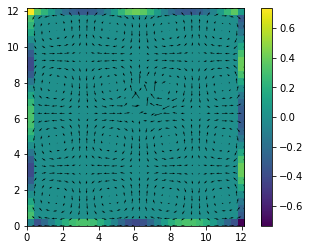
Figure 2: Simulation of modified Euler equations after $140$ time steps. The arrows represent the direction and magnitude of the fluid’s velocity. The color map shows the value of discrete divergence.

We can see in Figure 2 that due to incompressiblity of the fluid, the velocity field does not just ’flow out’ from the obstacle at $(7,7)$ in all directions. Instead, we can distinguish at least one direction along which the fluid accelerates towards the obstacle and eventually gets deviated to a second direction along which the fluid flows out of the obstacle.

V Conclusions and Future Work

We introduced modified Euler’s equations as solutions of an optimal control problem for the incompressible ideal flow of an inviscid fluid where we control the pressure of the fluid by means of an artificial potential function. In addition, we present simulation results for the necessary conditions of optimality in the optimal control problem by introducing the concept of discrete Helmholtz projection in order to obtain solutions with zero divergence.

In future work we aim to study the construction of geometric integrators preserving the qualitative behavior in simulations of the constraint of zero divergences by using the notion of discrete Helmholtz projection.

Finally, we would like to explore extensions of the obstacle avoidance problem for singular optimal control problems from a variational and geometric point of view in this context of infinite-dimensional configuration spaces. Such a setting arises for example in the optimal control of Maxwell equations for electromagnetism in a vacuum, and in the Maxwell-Vlasov systems for a collisionless plasma. Again a key goal is to use artificial potential functions to control the system.

Appendix A Auxiliary Lemmas

Lemma 1.

Let $\varphi:\Omega\times\mathbb{R}\to\Omega$ be a diffeomorphism for each fixed $t$, denote $v=\frac{\partial\varphi}{\partial t}\circ\varphi^{-1}$, and also let $z=\pi\circ\varphi^{-1}$, where $\pi:\Omega\times\mathbb{R}\to\mathbb{R}^{3}$. Then,

$$(T\pi\circ\varphi^{-1})\left(\frac{\partial\varphi^{-1}}{\partial t}\right)=-Tz(v)$$

Proof.

First, let us write an alternative expression for $\displaystyle{\frac{\partial\varphi^{-1}}{\partial t}}$. Indeed noting that $\varphi\circ\varphi^{-1}=\text{id}_{\Omega}$, we deduce that

$$\frac{\partial\varphi}{\partial t}\circ\varphi^{-1}+(T\varphi\circ\varphi^{-1})\left(\frac{\partial\varphi^{-1}}{\partial t}\right)=0.$$

Therefore,

$$(T\varphi\circ\varphi^{-1})\left(\frac{\partial\varphi^{-1}}{\partial t}\right)=-v$$

and, hence,

$$\frac{\partial\varphi^{-1}}{\partial t}=-(T\varphi\circ\varphi^{-1})^{-1}(v)=-T\varphi^{-1}(v).$$

Finally applying it the map $(T\pi\circ\varphi^{-1})$, we deduce

$$\begin{split}(T\pi\circ\varphi^{-1})\left(\frac{\partial\varphi^{-1}}{\partial t}\right)=&-(T\pi\circ\varphi^{-1})(T\varphi^{-1}(v))\\ =&-T(\pi\circ\varphi^{-1})(v)=-Tz(v).\end{split}$$

∎

Lemma 2.

Let $z:\Omega\times\mathbb{R}\to\mathbb{R}^{3}$ and $v:\Omega\times\mathbb{R}\to\mathbb{R}^{3}$ be two time-dependent vector fields on $\Omega\subseteq\mathbb{R}^{3}$. Then

1. $(Tv)^{T}z=(z\cdot\text{grad })v+z\times(\text{curl }v)$.

2. $Tz(v)=(v\cdot\text{grad })z$.

3. $(v\cdot\text{grad })z+(z\cdot\text{grad })v+z\times(\text{curl }v)=\text{grad }(v\cdot z)-v\times(\text{curl }z)$.

Proof.

1. Let us compute in coordinates $(z\cdot\text{grad })v+z\times(\text{curl }v)$ by denoting $z=(z_{1},z_{2},z_{3})$ and $v=(v_{1},v_{2},v_{3})$ and the coordinates in $\mathbb{R}^{3}$ by $(x_{1},x_{2},x_{3})$. Then,

   $$(z\cdot\text{grad })v=\left(z_{i}\frac{\partial v_{1}}{\partial x_{i}},z_{i}\frac{\partial v_{2}}{\partial x_{i}},z_{i}\frac{\partial v_{3}}{\partial x_{i}}\right)$$

   and

   $$\begin{split}z\times(\text{curl }v)=&\left(z_{2}\left(\frac{\partial v_{2}}{\partial x_{1}}-\frac{\partial v_{1}}{\partial x_{2}}\right)-z_{3}\left(\frac{\partial v_{1}}{\partial x_{3}}-\frac{\partial v_{3}}{\partial x_{1}}\right),\right.\\ &z_{3}\left(\frac{\partial v_{3}}{\partial x_{2}}-\frac{\partial v_{2}}{\partial x_{3}}\right)-z_{1}\left(\frac{\partial v_{2}}{\partial x_{1}}-\frac{\partial v_{1}}{\partial x_{2}}\right),\\ &\left.z_{1}\left(\frac{\partial v_{1}}{\partial x_{3}}-\frac{\partial v_{3}}{\partial x_{1}}\right)-z_{2}\left(\frac{\partial v_{3}}{\partial x_{2}}-\frac{\partial v_{2}}{\partial x_{3}}\right)\right)\end{split}$$

   Once, we add both vectors, most of the terms cancel out and we are left with

   $$\begin{split}(z\cdot\text{grad })v&+z\times(\text{curl }v)=\left(z_{i}\frac{\partial v_{i}}{\partial x_{1}},z_{i}\frac{\partial v_{i}}{\partial x_{2}},z_{i}\frac{\partial v_{i}}{\partial x_{3}}\right)\\ &=\begin{bmatrix}\frac{\partial v_{1}}{\partial x_{1}}&\frac{\partial v_{2}}{\partial x_{1}}&\frac{\partial v_{3}}{\partial x_{1}}\\ \frac{\partial v_{1}}{\partial x_{2}}&\frac{\partial v_{2}}{\partial x_{2}}&\frac{\partial v_{3}}{\partial x_{2}}\\ \frac{\partial v_{1}}{\partial x_{3}}&\frac{\partial v_{2}}{\partial x_{3}}&\frac{\partial v_{3}}{\partial x_{3}}\end{bmatrix}\begin{bmatrix}z_{1}\\ z_{2}\\ z_{3}\end{bmatrix}\\ &=\left(Tv\right)^{T}z\end{split}$$

2. It is straightforward, jsut notice that

   $$Tz(v) =\begin{bmatrix}\frac{\partial z_{1}}{\partial x_{1}}&\frac{\partial z_{1}}{\partial x_{2}}&\frac{\partial z_{1}}{\partial x_{3}}\\ \frac{\partial z_{2}}{\partial x_{1}}&\frac{\partial z_{2}}{\partial x_{2}}&\frac{\partial z_{2}}{\partial x_{3}}\\ \frac{\partial z_{3}}{\partial x_{1}}&\frac{\partial z_{3}}{\partial x_{2}}&\frac{\partial z_{3}}{\partial x_{3}}\end{bmatrix}\begin{bmatrix}v_{1}\\ v_{2}\\ v_{3}\end{bmatrix}$$

   $$=\left(v_{i}\frac{\partial z_{1}}{\partial x_{i}},v_{i}\frac{\partial z_{2}}{\partial x_{i}},v_{i}\frac{\partial z_{3}}{\partial x_{i}}\right).$$

3. This item can be found in the literature (see [16] or [17] for instance).

∎

References

- [1] A. M. Bloch, D. D. Holm, P. E. Crouch, and J. E. Marsden, “An optimal control formulation for inviscid incompressible ideal fluid flow,” in Proceedings of the 39th IEEE Conference on Decision and Control (Cat. No. 00CH37187), vol. 2. IEEE, 2000, pp. 1273–1278.
- [2] V. Arnold, “Sur la géométrie différentielle des groupes de lie de dimension infinie et ses applications à l’hydrodynamique des fluides parfaits,” in Annales de l’institut Fourier, vol. 16, no. 1, 1966, pp. 319–361.
- [3] J. Marsden and A. Weinstein, “Coadjoint orbits, vortices, and clebsch variables for incompressible fluids,” Physica D: Nonlinear Phenomena, vol. 7, no. 1-3, pp. 305–323, 1983.
- [4] D. G. Ebin and J. E. Marsden, “Groups of diffeomorphisms and the solution of the classical euler equations for a perfect fluid,” 1969.
- [5] J. E. Marsden, T. Raţiu, and A. Weinstein, “Semidirect products and reduction in mechanics,” Transactions of the american mathematical society, vol. 281, no. 1, pp. 147–177, 1984.
- [6] D. D. Holm, “Euler’s fluid equations: Optimal control vs optimization,” Physics Letters A, vol. 373, no. 47, pp. 4354–4359, 2009.
- [7] A. M. Bloch and P. E. Crouch, “Optimal control and geodesic flows,” Systems & control letters, vol. 28, no. 2, pp. 65–72, 1996.
- [8] A. M. Bloch, R. W. Brockett, and P. E. Crouch, “Double bracket equations and geodesic flows on symmetric spaces,” Communications in mathematical physics, vol. 187, pp. 357–373, 1997.
- [9] A. M. Bloch, P. E. Crouch, J. E. Marsden, and T. S. Ratiu, “Discrete rigid body dynamics and optimal control,” in Proceedings of the 37th IEEE Conference on Decision and Control (Cat. No. 98CH36171), vol. 2. IEEE, 1998, pp. 2249–2254.
- [10] A. Bloch, M. Camarinha, and L. J. Colombo, “Variational obstacle avoidance on riemannian manifolds,” Proceedings of the 2017 IEEE International Conference on Decision and Control, pp. 146–150, 2017.
- [11] ——, “Dynamic interpolation for obstacle avoidance on riemannian manifolds,” International Journal of Control, vol. 94, no. 3, pp. 588–600, 2021.
- [12] M. Assif, R. Banavar, A. Bloch, M. Camarinha, and L. J. Colombo, “Variational collision avoidance problems on riemannian manifolds,” Proceedings of the 2018 IEEE International Conference on Decision and Control, pp. 2791–2796, 2018.
- [13] R. Chandrasekaran, L. J. Colombo, M. Camarinha, R. Banavar, and A. Bloch, “Variational collision and obstacle avoidance of multi-agent systems on riemannian manifolds,” Proceedings of the 2020 European Control Conference, 2020.
- [14] A. Bloch, M. Camarinha, and L. J. Colombo, “Variational point-obstacle avoidance on riemannian manifolds,” Mathematics of Control, Signals, and Systems, vol. 33, pp. 109–121, 2021.
- [15] D. D. Holm, J. E. Marsden, and T. S. Ratiu, “The euler–poincaré equations and semidirect products with applications to continuum theories,” Advances in Mathematics, vol. 137, no. 1, pp. 1–81, 1998.
- [16] L. Brand, Vector and tensor analysis. Courier Dover Publications, 2020.
- [17] J. E. Marsden, A. J. Tromba, A. Weinstein et al., Basic multivariable calculus. Springer, 1993.
- [18] F. Gay-Balmaz, D. Holm, and T. Ratiu, “Geometric dynamics of optimization,” Communications in Mathematical Sciences, vol. 11, no. 1, pp. 163–231, 2013.
- [19] R. Abraham and J. E. Marsden, Foundations of mechanics. American Mathematical Soc., 2008, no. 364.
- [20] R. Abraham, J. E. Marsden, and T. Ratiu, Manifolds, tensor analysis, and applications. Springer Science & Business Media, 2012, vol. 75.
- [21] O. Khatib, “Real-time obstacle avoidance for manipulators and mobile robots,” The international journal of robotics research, vol. 5, no. 1, pp. 90–98, 1986.
- [22] D. E. Koditschek, “Robot planning and control via potential functions,” The robotics review, p. 349, 1989.
- [23] A. J. Chorin and J. E. Marsden, A Mathematical Introduction to Fluid Mechanics, 2nd ed., ser. Texts in Applied Mathematics. Springer New York, NY, 1990, originally published in the series: Universitext. [Online]. Available: https://doi.org/10.1007/978-1-4684-0364-0
- [24] H. Bhatia, G. Norgard, V. Pascucci, and P.-T. Bremer, “The helmholtz-hodge decomposition—a survey,” IEEE Transactions on Visualization and Computer Graphics, vol. 19, no. 8, pp. 1386–1404, 2013.
- [25] D. Pavlov, P. Mullen, Y. Tong, E. Kanso, J. Marsden, and M. Desbrun, “Structure-preserving discretization of incompressible fluids,” Physica D: Nonlinear Phenomena, vol. 240, no. 6, pp. 443–458, 2011. [Online]. Available: https://www.sciencedirect.com/science/article/pii/S0167278910002873