Probing the disc-jet coupling in S4 0954+65, PKS 0903-57, $\&$ 4C +01.02 with $\gamma$-rays

Abstract

We present a comprehensive variability study on three blazars, S4 0954+65, PKS 0903-57, and 4C +01.02 covering a mass range of log(M/M_⊙) = 8–9, by using $\sim$15 years-long $\gamma$-ray light curves from Fermi-LAT. The variability level is characterized by the fractional variability amplitude which is higher for $\gamma$-rays compared to optical/UV and X-rays emissions. A power spectral density (PSD) study and damped random walk (DRW) modeling are done to probe the characteristic timescale. The PSD is fitted with a single power-law (PL) and bending power-law models and the corresponding success fraction was estimated. In the case of PKS 0903-57, We observed a break in the $\gamma$-ray PSD at 256 days which is comparable to the viscous timescale in the accretion disc suggesting a possible disk-jet coupling. The non-thermal damping timescale from the DRW modeling is compared with the thermal damping timescale for AGNs including our three sources. Our sources lie on the best-fit of the $\mathrm{\tau^{rest}_{damping}}-M_{BH}$ plot derived for AGN suggesting a possible accretion disc-jet connection. If the jet’s variability is linked to the disc’s variability, we expect a log-normal flux distribution, often connected to the accretion disc’s multiplicative processes. Our study observed a double log-normal flux distribution, possibly linked to long and short-term variability from the accretion disk and the jet. In summary, PSD and DRW modeling results for these three sources combined with blazars and AGNs studied in literature favor a disc-jet coupling scenario. However, more such studies are needed to refine this understanding.

1 Introduction

Active galactic nuclei (AGN) are the most luminous sources in the universe, hosting supermassive black holes (SMBHs) at their centers. These extraordinary astronomical sources have been studied for more than half a century (Matthews & Sandage, 1963), and can be distinguished and identified through a range of factors, including their bolometric luminosity ($L\sim 10^{47}ergs^{-1}$), flux variabilities, and spectral energy distribution (SEDs), etc. The immense luminosity from AGN arises from the accretion of matter around the SMBHs. This process serves as the primary source of energy that powers the AGN. Flux variability involves non-periodic variations in flux, which occur on various timescales and exhibit different amplitudes. Only a small fraction of AGN show radio emissions and are called radio-loud AGN. Some of these AGN have relativistic jets pointed towards Earth and are known as Blazars (Urry & Padovani, 1995). These sources are known to exhibit extreme properties such as high-energy emission, and rapid and large amplitude flux variations in the entire accessible spectral range (Ulrich et al., 1997). Blazars are also sources of non-thermal emissions, which undergo Doppler boosting due to their relativistic jets.

Multi-frequency variability studies have emerged as a vital tool for gaining valuable insights into the physical conditions prevailing within the innermost regions of blazars. These studies provide a means to investigate various aspects of blazars, such as the dominant particle acceleration mechanism, energy dissipation processes, magnetic field geometry, and the composition of the jet. The flux variability is classified into sub-categories: long-term variability, occurring over timescales of decades/years to several months; short-term variability, manifesting within weeks to days; and intranight variability, which transpires within a single day (Ulrich et al., 1997). The power spectral densities (PSDs) from blazar light curves often exhibit a distinctive pattern characterized by a single power-law shape, represented by a form $P(\nu_{k})\propto\nu_{k}^{-\beta}$, where $\beta$ denotes the slope of the power-law function, while $\nu_{k}$ represents the temporal frequencies. This behavior indicates that the observed variability follows a colored noise-type stochastic process (Finke & Becker, 2014; Goyal et al., 2017). Specifically, different values of $\beta$ offer insights into distinct types of stochastic processes. For instance, when $\beta\simeq$ 1, $\beta\simeq$ 2, and $\beta\gtrsim$ 3, we observe long memory/pink-noise, damped walk/red-noise, and black noise-type stochastic processes, respectively. While $\beta\sim$ 0 represents uncorrelated white-noise type stochastic process (Press, 1978). Fluctuations arising from the stochastic process follow certain probability distributions, which impart predictability to the PSDs. Therefore, the PSD of the light curves holds valuable information about the parameters of the stochastic process and the characteristic/relaxation timescales governing the variability in the system. By examining the slope, normalization, and breaks in the PSD, we can glean insights into various aspects, such as the timescales associated with particle cooling or escape (Kastendieck et al., 2011; Sobolewska et al., 2014; Finke & Becker, 2014; Chen et al., 2016; Kushwaha et al., 2017; Chatterjee et al., 2018; Ryan et al., 2019; Bhattacharyya et al., 2020). Significant efforts have been made to model the complex phenomena related to the multi-waveband variability/SED observed in the sources. These models encompass a diverse range of physical processes that occur either within the accretion disc or the jets. The proposed scenarios explore emission sites located in the accretion disc, which revolves around a supermassive black hole, magneto-hydrodynamic instabilities within the disc and jets, the propagation of shocks downstream in relativistic jets, as well as the relativistic effects resulting from the orientation of the jet. These models aim to capture the intricate mechanisms responsible for the observed variability, taking into account the interplay between the accretion disc and the jet and their influence on the emission across different wavebands (Camenzind & Krockenberger, 1992; Wagner & Witzel, 1995; Marscher, 2013). However, the precise study of the underlying processes is still a subject of ongoing debate and investigation.

Extensive studies utilizing large datasets across various wavebands have been conducted to characterize the properties of PSDs over a wide range of timescales, spanning from days to years. At the radio frequencies, Park & Trippe (2017); Max-Moerbeck et al. (2014) analyzed decades-long radio data and reported $\beta\sim$ 1-3. At optical frequencies, Nilsson et al. (2018); Goyal (2021) reported $\beta\sim$ 1-1.5. In the X-ray waveband, Kataoka et al. (2001); Isobe et al. (2014); Chatterjee et al. (2018) reported $\beta\sim$ 1-1.5. Studies in the high-energy $\gamma$-rays domain, (Abdo et al., 2010; Meyer et al., 2019; Bhatta & Dhital, 2020; Tarnopolski et al., 2020) reported $\beta\sim$ 1-2. In the very high-energy $\gamma$-ray domain, Goyal (2020) reported $\beta\sim$ 1 for couple of blazars.

Another approach involves fitting stochastic light curves using Gaussian processes in the time domain (Kelly et al., 2009; Li & Wang, 2018; MacLeod et al., 2010). This approach has gained considerable traction in characterizing the optical variability of AGNs. A notable representation of such processes is the Continuous-time Autoregressive Moving Average (CARMA) models developed by Kelly et al. (2014). The damped random walk (DRW) model, also represented by CARMA(1,0), has demonstrated its efficacy in accurately characterizing the long-term variability of the AGN accretion discs (Kelly et al., 2009; Kozłowski et al., 2009; Zu et al., 2013; Rakshit & Stalin, 2017; Kasliwal et al., 2017; Lu et al., 2019; Burke et al., 2021). These stochastic processes have proven to be powerful methods for probing AGN variability with remarkable success. Recent advances have extended the utility of the CARMA model to the realm of $\gamma$-ray variabilities of AGN (Sobolewska et al., 2014; Goyal et al., 2018; Ryan et al., 2019; Tarnopolski et al., 2020; Covino et al., 2020; Yang et al., 2021; Zhang et al., 2022). This extension has demonstrated the ability to capture features of the flux variability and to provide a more accurate representation of the PSD. In addition to CARMA, Foreman-Mackey et al. (2017) developed another fast and flexible method for light curve modeling with a stochastic process, celerite. With access to almost 15 years of Fermi-LAT data, it provides an opportunity to comprehensively study the $\gamma$-ray light curves of AGN. This endeavor allows us to thoroughly investigate and reveal the inherent stochastic properties through well-established methods.

The main objective of this study is to comprehensively examine and understand the disk-jet coupling in blazar. To achieve this, we conduct an extensive investigation utilizing 15 years long data from the Fermi-LAT $\&$ Swift-XRT/UVOT observations. We focus on three selected blazars S4 0954+65, PKS 0903-57, and 4C +01.02 of different types (BL Lacertae [BL Lac], Blazar Candidates of Uncertain class [BCU], and Flat Spectrum Radio Quasar [FSRQ]) and covering a mass range from 10⁸ to 3$\times$10⁹ M_⊙. In section 2, the data analysis methods for Fermi-LAT and Swift-XRT/UVOT are outlined. In section 3, A variety of analysis approaches have been used to comprehensively investigate the broadband light curves. These methods include fractional variability, flux distribution, PSD, and DRW modeling analyses, and the obtained results are detailed in corresponding sections. In section 4, we discuss the obtained results in detail. Finally, A comprehensive conclusion is presented in Section 5.

2 MULTI-WAVELENGTH OBSERVATIONS AND DATA ANALYSIS

In this investigation, a sample of blazars (S4 0954+65, PKS 0903-57, and 4C +01.02) has been selected for a comprehensive study of multi-waveband variability within the time span of MJD 54683 - 59970. These sources are positioned at (RA: 149.69, Dec: 65.56) for S4 0954+65 with redshift, z $\sim$ 0.367 (Lawrence et al., 1986, 1996; Stickel et al., 1993), (RA: 136.22, Dec: -57.58) for PKS 0903-57 with z $\sim$ 0.695 (Thompson et al., 1990), and (RA: 17.16, Dec: 1.58) for 4C +01.02 with z $\sim$ 2.099 (Hewett et al., 1995). The BH mass of S4 0954+65 is $\sim 3.3\times 10^{8}M_{\odot}$, estimated from the width of the H_α line (Fan & Cao, 2004). For 4C +01.02, a BH mass of $\sim 3\times 10^{9}M_{\odot}$ was found through SED and spectropolarimetry modeling (Schutte et al., 2022). For PKS 0903-57, we did not find an estimated BH mass value. However, we have adopted the most probable BH mass value between $3-6\times 10^{8}M_{\odot}$ from the distribution of BH mass of all radio-loud AGN from Ghisellini & Tavecchio (2015).

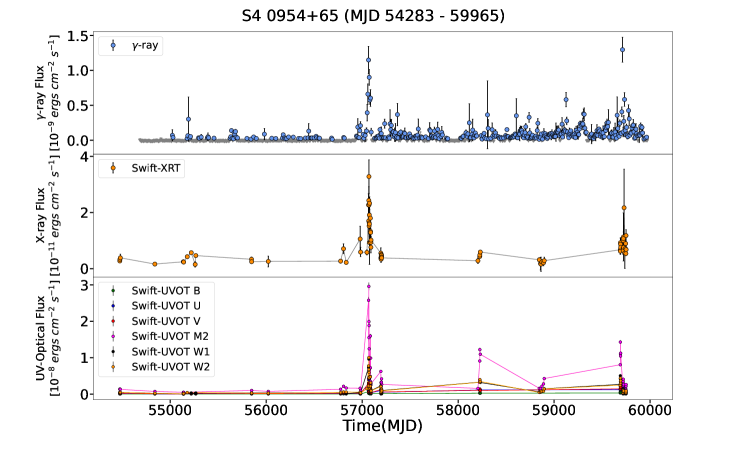
Figure 1: The multi-wavelength light curve of blazar S4 0954+65 in the time domain MJD 54283 - 59965. The top panel displays the weekly binned $\gamma$-ray light curve obtained from Fermi-LAT data. The grey points represent the upper limits. The middle panel presents the X-ray light curve generated using all available observation IDs from July 2007 to January 2022. Finally, the bottom panel shows the light curves for all Swift-UVOT bands (V, B, U, UVM2, UVW1, UVW2), which were generated from the same observations as the Swift-XRT data.

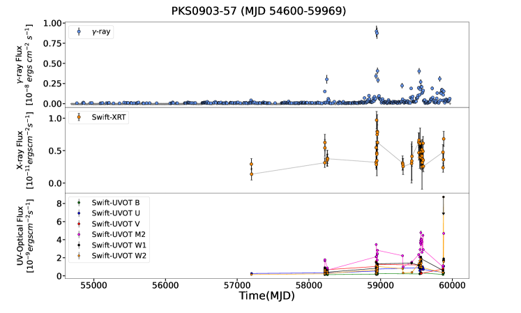
Figure 2: Shows the multi-wavelength light curve of the blazar PKS 0903-57 in the time domain MJD 54600 - 59969. The top panel displays the weekly binned $\gamma$-ray light curve obtained from Fermi-LAT data. The grey points represent the upper limits. The middle panel presents the X-ray light curve generated using all available observation IDs from May 2008 to January 2023. Finally, the bottom panel shows the light curves for all Swift-UVOT bands (V, B, U, UVM2, UVW1, UVW2), which were generated from the same observations as the Swift-XRT data.

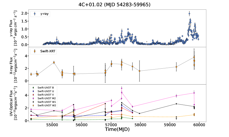
Figure 3: Shows the multi-wavelength light curve of 4C +01.02 in the time domain MJD 54283 - 59965. The top panel displays the weekly binned $\gamma$-ray light curve obtained from Fermi-LAT data. The grey points represent the upper limits. The middle panel presents the X-ray light curve generated using all available observation IDs from July 2007 to January 2023. Finally, the bottom panel shows the light curves for all Swift-UVOT bands (V, B, U, UVM2, UVW1, UVW2), which were generated from the same observations as the Swift-XRT data.

2.1 Fermi-LAT

The Fermi $\gamma$-ray Space Telescope was launched in June 2008 aboard the Delta-II rocket. It has two instruments onboard: the Large Area Telescope (LAT) and the $\gamma$-ray Burst Monitor (GBM). LAT has a maximum effective area of 9500 $cm^{2}$ at normal incidence in the 1-10 GeV energy range. It has a field of view (FoV) of 2.4 sr and angular resolution at 100 MeV is < $3.5^{\circ}$ and < $0.15^{\circ}$ at 10 GeV.

Fermi-LAT started collecting data from MJD 54682.655 (4th Aug 2008). Therefore, we considered the data starting from MJD 54683 to MJD 59970 (26 January 2023). We used the FermiPy (Wood et al., 2017) package in Python for the analysis which leverages the Fermi Science Tools. The FermiPy package requires us to define all the analysis and data selection parameters in a YAML configuration file. The energy range of 100 MeV to 300 GeV and a circular region of interest of size 10 degrees was considered for the analysis for all the sources in the same period MJD 54683-59970. Further, the data were filtered using the constraints evclass=128 and evtype=3 for gtselect. The zenith angle cut-off of 90 degrees was chosen. The filter ’(DATA_QUAL>0)&&(LAT_CONFIG==1)’ was used for the gtmktime tool. The Galactic interstellar emission model (IEM) and isotropic diffuse emission template used for the analysis are gll_iem_v07.fits and iso_P8R3_SOURCE_V3_v1.txt respectively.

FermiPy uses the GTAnalysis python class which has various functions for analyses and computations. The $\gamma$-ray light curves are generated with 7-day binning using the lightcurve function of GTAnalysis class.

2.2 Swift-XRT

In November 2004, NASA launched the Neil Gehrels Swift observatory equipped with three instruments: the Burst Alert Telescope (BAT), the X-Ray Telescope (XRT), and the Ultra-violet Optical Telescope (UVOT). The XRT instrument (Burrows et al., 2005), designed as a grazing incidence Wolter-1 telescope, boasts an impressive effective area of about 110 $cm^{2}$ and is capable of detecting X-rays in the energy range of 0.3 to 10 keV.

In this study, we made use of the Swift observations that were available in the same time frame as the Fermi observations. Specifically, we analyzed 77 Swift-XRT observations taken between MJD 54475 to 59750 for S4 0954+65, 52 observations from MJD 57197 to 59878 for PKS 0903-57, and 25 observations from MJD 54283 to 59831 for 4C +01.02.

To analyze the X-ray data, we focused on the energy range of 0.3-8.0 keV and used the tools from the HEASOFT package (v6.31). Initially, we used the xrtpipeline package (v0.13.7) to generate clean event files (or Level 2 products) from the raw data. These Level 2 products were used to select the source and background events from circular regions with radii of 50-arcsec and 100-arcsec, respectively, in the DS9 viewer. The next step involved extracting the light curves and spectrum from the source and background events using the xselect (v2.5b) tool . During the analysis of the XRT data, we observed that six observations of PKS 0903-57 and 23 observations of S4 0954+65 had piled-up events. These observations were promptly corrected before generating the XRT products. To solve this problem, we used an annulus region instead of a circular region to extract the light curve and spectrum. The annulus region allowed us to exclude the core of the point spread function (PSF), which was involved in the piled-up events.

The redistribution matrix file (RMF) was obtained from the HEASARC calibration database. The ancillary response files (ARF) were generated using the xrtmkarf tool. While generating the ARF file, the PSF was set to yes, which allowed the creation of an ARF-corrected file to compensate for the loss of counts resulting from the annulus exclusion. The tool grppha was used to combine the source and background event files, the auxiliary response file, and the redistribution matrix file into a single spectrum file. The spectrum was fitted with a simple power-law model $F(E)=KE^{\Gamma_{x}}$ using XSPEC (v12.13.0c). During the fitting process, we used $N_{H}$ values (Ahnen et al., 2018; Shah et al., 2021; Malik et al., 2022) of 5.17$\times 10^{20}cm^{-2}$, 2.6$\times 10^{21}cm^{-2}$, and 2.25$\times 10^{20}cm^{-2}$ for S4 0954+65, PKS 0903-57, and 4C +01.02, respectively.

2.3 Swift-UVOT

The Swift Observatory’s Ultra-violet Optical Telescope (Roming et al. 2005) has the capability of detecting UV and optical radiation simultaneously. We acquired data in three optical filters (V, B, and U bands) and three UV filters (W1, M2, and W2 bands) over the same period in which the Swift-XRT observations were obtained. The uvotsource tool was used to obtain the magnitudes. Then the magnitudes were corrected for galactic extinction $A_{\lambda}$ and reddening by considering a value of E(B-V) = 0.397 (Schlafly & Finkbeiner 2011) and calculated the $A_{\lambda}$ (Giommi et al. 2006) for all filters used. To obtain flux measurements, we converted the corrected magnitudes using appropriate conversion factors, dust absorption relation $Mag_{0}=Mag-A_{\lambda}$, and zero-point magnitude relation (Breeveld et al. 2011) given as $Z_{pt}=-2.5log(F)-Mag_{0}$, where $Z_{pt}$ is Zero point magnitude and F is the flux density in the units of $ergcm^{-2}s^{-1}$/Å. To generate the multi-waveband light curve, we used the given procedure as above using the uvotsource tool. For constructing the SED, all the image files were combined using the uvotimsum tool.

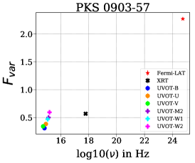
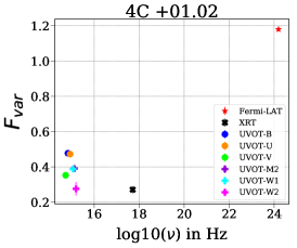
Figure 4: The fractional variability was computed for each observed waveband (Table-1). The left, middle, and right panel shows the variability levels for source S4 0954+65, PKS 0903-57, and 4C +01.02, respectively.

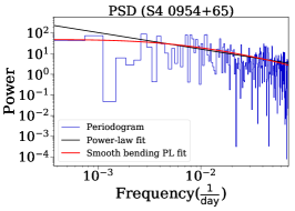
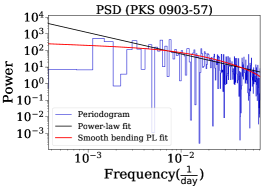
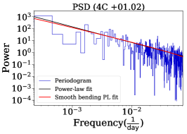
Figure 5: The PSD of the $\gamma$-ray light curves, which were fitted with a power-law (black solid line) and a smooth bending power-law model (red solid line).

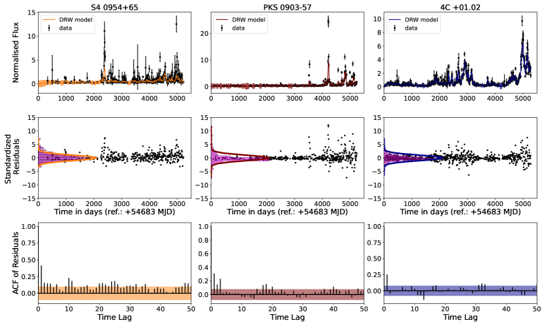
Figure 6: The figure showcases the outcomes of DRW modeling applied to the 7-day binned $\gamma$-ray lightcurves of three distinct sources: S4 0954+65 (left column), PKS 0903-57 (middle column), and 4C +01.02 (right column). In the top row, the observed LAT data points (black points), with associated errors. The DRW best fits are displayed as bright orange, maroon, and blue lines, for the three sources, respectively. In the middle row, we visualize the standardized residuals of each bin, the magenta histogram shows the scaled distribution of standardized residuals, while the orange, maroon, and blue solid lines represent the scaled normal distributions in these sources. Finally, the bottom row features the autocorrelation functions (ACFs) of the residuals with 95$\%$ confidence limits of the white noise.

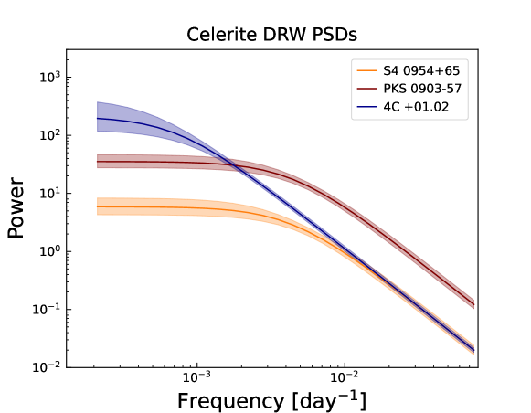
Figure 7: The PSDs of $\gamma$-ray light curves constructed from the Celerite DRW modeling results for three sources are depicted in this figure: S4 0954+65 (in orange), PKS 0903-57 (in brown), and 4C +01.02 (in blue). The shaded regions in corresponding colors encompass the 1$\sigma$ confidence intervals.

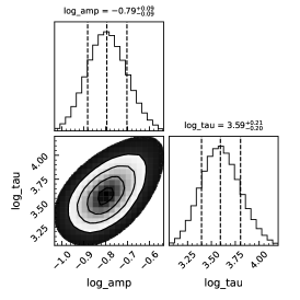
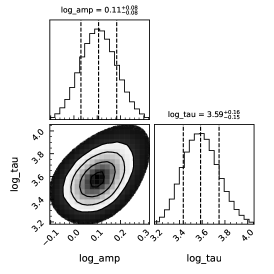
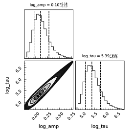
Figure 8: The posterior probability densities of the DRW model parameters for all three blazars. The left panel corresponds to source S4 0954+65, the middle panel represents PKS 0903-57, and the right panel pertains to 4C +01.02.

3 Methodologies and Results

In order to comprehensively study the statistical variability characteristics of the selected blazars, an in-depth study of the $\gamma$-ray light curve was carried out by applying various analysis methods including fractional variability, PSD analysis, DRW modeling and flux-distribution along with extensive Monte Carlo (MC) simulations. The details of the analysis methods and corresponding results are presented in the following sections.

3.1 Fractional Variability

The long-term broadband light curves for all three sources are produced and shown in Figure 1, 2, & 3. Over the long period, multiple flaring states are observed which are also accompanied by X-ray and optical-UV.

The variability intensity of a light curve $x_{i}$ with N data points can be quantified using its variance, which can be defined as

$$S^{2}=\frac{1}{(N-1)}\sum_{i=1}^{N}(\langle x\rangle-x_{i})^{2}$$ (1)

However, when dealing with blazar light curves, finite uncertainties $\sigma_{err,i}$ arise from measurement errors, such as Poisson noise in photon counting. These uncertainties in the individual flux measurements introduce additional variance in estimating the source’s variability. To accurately assess the intrinsic variability of the source, it is crucial to account for the effect of measurement noise. This is achieved by calculating the excess variance ($\sigma_{XS}$), which represents the variance of the light curve after subtracting the contribution caused by measurement uncertainties (Nandra et al., 1997; Edelson et al., 2002)

$$\sigma_{XS}^{2}=S^{2}-\overline{\sigma_{err}^{2}},$$ (2)

where, $\overline{\sigma_{err}^{2}}$ is the mean square error, which can be defined as

$$\overline{\sigma_{err}^{2}}=\frac{1}{N}\sum_{i=1}^{N}\sigma_{err,i}^{2}$$ (3)

The excess variance serves as an estimator of the intrinsic source variance. Additionally, the fractional variability amplitude ($F_{var}$) is defined as the square root of the normalized excess variance, which is given as, $\sigma_{NXS}^{2}=\frac{\sigma_{XS}^{2}}{\overline{x}^{2}}$. It measures the level of intrinsic variability relative to the square of the mean flux measurement, providing valuable insights into the source’s variability characteristics. The expression for $F_{var}$ (Vaughan et al., 2003) is given as

$$F_{var}=\sqrt{\frac{S^{2}-\overline{\sigma_{err}^{2}}}{\overline{x}^{2}}}$$ (4)

The parameter $F_{var}$ provides a measure of the percentage of variability amplitude and is determined by a linear statistic. The uncertainty on excess variance (Vaughan et al. 2003) is given by

$$err(\sigma_{NXS}^{2})=\sqrt{\left(\sqrt{\frac{2}{N}}\cdot\frac{\overline{\sigma_{err}^{2}}}{\overline{x}^{2}}\right)^{2}+\left(\sqrt{\frac{\overline{\sigma_{err}^{2}}}{N}}\cdot\frac{2F_{var}}{\overline{x}}\right)^{2}}$$ (5)

and the uncertainty of $F_{var}$ (Poutanen et al. 2008; Bhatta & Webb 2018) is given by

$$\Delta F_{var}=\sqrt{F_{var}^{2}+err\left(\sigma_{NXS}^{2}\right)}-F_{var}$$ (6)

The fractional variability amplitude was computed across all observed wavebands, and obtained Fvar values are included in Table 1. The Fvar is plotted as a function of energy in Figure 4. The UV and $\gamma$-ray emission appear to be more variable in S4 0954+65 compared to optical and X-rays. In PKS 0903-57 and 4C +01.02 the $\gamma$-ray emission is highly variable compared to optical-UV and X-ray emission. This resembles the variability pattern in other blazars as seen in Rani et al. (2016); Prince et al. (2022), & Abdo et al. (2011). It is also suggested that in some of the cases, the variability pattern resembles the shape of the broadband SED (Aleksić et al., 2015a, b).

Wavebands	$F_{var}$
	S4 0954+65	PKS 0903-57	4C +01.02
Fermi-LAT	1.1 $\pm$ 0.03	2.27 $\pm$ 0.013	1.18 $\pm$ 0.01
Swift-XRT	1.03 $\pm$ 0.001	0.57 $\pm$ 0.01	0.27 $\pm$ 0.02
UVOT-W2	1.12 $\pm$ 0.006	0.59 $\pm$ 0.008	0.27 $\pm$ 0.03
UVOT-M2	1.12 $\pm$ 0.008	0.50 $\pm$ 0.009	0.39 $\pm$ 0.019
UVOT-W1	1.13 $\pm$ 0.006	0.47 $\pm$ 0.008	0.38 $\pm$ 0.016
UVOT-U	1.026 $\pm$ 0.004	0.38 $\pm$ 0.005	0.47 $\pm$ 0.011
UVOT-B	1.025 $\pm$ 0.004	0.31 $\pm$ 0.005	0.477 $\pm$ 0.014
UVOT-V	0.99 $\pm$ 0.004	0.34 $\pm$ 0.005	0.35 $\pm$ 0.015

Table 1: Fractional variability ($F_{var}$) in different wavebands. The energy range for Fermi-LAT is 0.1–300 GeV and for Swift-XRT is 0.3 - 10 keV.

3.2 Power Spectral Density

The variability in the AGN light curve can also be characterized by the PSD. It determines the amplitude of variations and quantifies the power emitted at various frequencies. In the case of a regularly sampled time series, the PSD can be obtained by taking the modulus squared of its discrete Fourier transform (DFT). This approach allows us to analyze the frequency content of the data and determine the power associated with different frequencies. The discrete Fourier transform (DFT) of the set $\{x_{k}\}_{k=1,..,N}$ is

$$DFT(f_{s})=\sum_{k=1}^{N}x_{k}exp[-2\pi if_{s}t_{k}]$$ (7)

where the discrete set of frequencies is given as, $f_{s}=\frac{s-1}{N\delta t},s\in{1,..,N}$, and $\delta t=t_{k+1}-t_{k}$ is a constant time interval between consecutive observations. The sampling rate, denoted as SR, can be defined as the reciprocal of the time interval, denoted as $\delta t$. Mathematically, we express this relationship as $SR=1/\delta t$. Furthermore, the Nyquist frequency, denoted as $f_{Nyq}$, is equal to half of the sampling rate, or $1/2\delta t$. The rms-normalized PSD is defined as

$$P(f_{s})=\frac{2\delta t}{N}|DFT(f_{s})|^{2}$$ (8)

In the frequency range, only half of the N frequencies are physically meaningful. The Poisson noise floor level resulting from measurement uncertainties can be expressed as

$$P_{poisson}=\frac{2\delta t}{N}\sum_{k=1}^{N}\Delta x_{k}^{2}$$ (9)

This analysis aims to identify any notable peaks or breaks in the source PSD, which could suggest the presence of characteristic time scales specific to the system. Consequently, two distinct models (Timmer & Koenig, 1995; Emmanoulopoulos et al., 2013), a smoothly broken power law and a simple power law were employed to fit the PSD and identify the characteristic features. Both models can be expressed by the given equations,

The simple power-law model,

$$P(f)=P_{norm}f^{-\beta}$$ (10)

and, the bending power-law model,

$$P(f)=\frac{P_{norm}f^{-\beta_{1}}}{1+\left(\frac{f}{f_{break}}\right)^{\beta_{2}-\beta_{1}}}+C$$ (11)

where parameter C represents an estimation of the Poisson noise level originating from the uncertainties associated with individual measurements. The power-law model is characterized by the parameter $\beta$, while the smoothly broken power-law model involves two indices, $\beta_{1}$ and $\beta_{2}$, which correspond to low and high frequencies, respectively. The break frequency, denoted as $f_{break}$, is used to calculate the break timescale, represented as $T_{break}$, where $T_{break}$ = 1/$f_{break}$.

The Emmanoulopoulos algorithm, a combination of the Timmer-Koenig (TK95; Timmer & Koenig 1995) and Schreiber & Schmitz (SS96; Schreiber & Schmitz 1996) methods, was utilized to generate synthetic light curves by incorporating the underlying PSD and Probability Density Function (PDF) of the observed light curve. To assess the significance of the observed PSD, we employed Monte Carlo simulation. This involves generating a PSD of the synthetic light curves using the Fourier transform described above. By calculating the mean power and standard deviation of the PSD at each unique frequency, we were able to investigate the significance level of the PSD.

In order to evaluate the model’s goodness of fit, simulated light curves were used. These simulated light curves were rebinned to mimic the observed data and subjected to Fourier transformation in exactly the same way as the observed data. The assessment of the model’s fit is based on the construction of two statistical functions (Goyal et al., 2022), similar to $\chi^{2}$ statistics, defined as

$$\chi_{obs}^{2}=\sum_{\nu_{k}=\nu_{min}}^{\nu_{max}}\frac{[PSD(\nu_{k})_{obs}-\overline{PSD(\nu_{k})_{sim}}]^{2}}{(\Delta\overline{PSD(\nu_{k})_{sim}})^{2}}$$ (12)

and,

$$\chi_{dist,i}^{2}=\sum_{\nu_{k}=\nu_{min}}^{\nu_{max}}\frac{[PSD(\nu_{k})_{sim,i}-\overline{PSD(\nu_{k})_{sim}}]^{2}}{(\Delta\overline{PSD(\nu_{k})_{sim}})^{2}}$$ (13)

In the equations, $PSD(\nu_{k})_{obs}$ represents the observed PSD, while $PSD(\nu_{k})_{sim,i}$ corresponds to the simulated PSD obtained from the simulated light curves. $\overline{PSD(\nu_{k})_{sim}}$ denotes the mean, and $\Delta PSD(\nu_{k})_{sim}$ represents the standard deviation, calculated by averaging the numerous PSDs generated. Here, the variable k pertains to the unique frequencies within the PSD, while the index i spans over the number of simulated light curves. The $\chi_{obs}^{2}$ represents the minimum $\chi^{2}$ value obtained when comparing the model to the actual data. The $\chi_{dist}^{2}$ values are used to evaluate the goodness of fit associated with the $\chi_{obs}^{2}$. It is important to note that neither the $\chi_{dist,i}^{2}$ nor the $\chi_{obs}^{2}$ follow a standard $\chi^{2}$ distribution. Hence, to determine the acceptance or rejection of a model for a specific simulated light curve, the $\chi_{dist,i}^{2}$ values were compared to the $\chi_{obs}^{2}$. To achieve this, the $\chi_{dist,i}^{2}$ values were sorted in ascending order. The model was considered acceptable if the $\chi_{dist,i}^{2}$ was greater than the $\chi_{obs}^{2}$. The success fraction, which indicates the goodness of fit in terms of capturing the shape and slope of the intrinsic PSD, is defined as the ratio of m to M. Here, m represents the count of the number of $\chi_{dist,i}^{2}$ values that are greater than the $\chi_{obs}^{2}$ value, while M denotes the total number of PSDs obtained from the simulated light curves. The success fraction is also commonly referred to as the $p_{\beta}$ (Uttley et al. 2002; Chatterjee et al. 2008). A high value of $p_{\beta}$ or a large success fraction indicates a good fit to the PSD, indicating that a substantial proportion of randomly generated realizations capture the desired characteristics of the intrinsic PSD and providing insight into the likelihood of a model being accepted.

Following the above steps we produced the PSD of all three blazars for $\gamma$-ray, X-ray, and optical/UV. Due to the bad sampling of data in X-ray and optical/UV, we could not recover the good PSD, and the results are not shown here. For $\gamma$-ray, the PSD is generated in the frequency range of $10^{-4}-10^{-1}$ day^-1 and fitted with both a power-law and bending power law model. The fitted parameters and the corresponding plots are shown in Table 2 and Figure 5. We have computed the Akaike Information Criterion (AIC) and Bayesian Information Criterion (BIC) values to determine the best-fit model for the PSD of all sources. The results are detailed in Table 2. It is evident from the AIC or BIC values that the bending power-law model provides the best fit for the PSD of all sources. In addition, We also estimate the success fraction (SF) in order to find out the goodness of the fit. A high value of SF indicates a good fit. We noticed that the bending power-law model provides the most favorable fit to the PSDs of all the sources. Moreover, the outcomes of the success fraction provide additional support for this conclusion.
In the case of blazar S4 0954+65, we observed a PSD break of 212 days ($\sim$0.0047 $\mathrm{days}^{-1}$). Similarly, for blazar PKS 0903-57 and 4C +01.02, the PSD break is observed at 256 days ($\sim$0.0039 $\mathrm{days}^{-1}$) and 714 days ($\sim$0.0014 $\mathrm{days}^{-1}$). The break in the high-energy PSD is observed only in a handful of blazars before (Ryan et al., 2019). The details about the other fitted parameters are shown in Table  2.

Model	Parameter	S4 0954+65	PKS 0903-57	4C +01.01
Power-law	Normalisation constant	0.41	0.16	0.01
	Slope	0.80	1.28	1.32
	Success-fraction	48.4$\%$	24.7$\%$	40$\%$
	AIC	1691.80	2794.40	3576.93
	BIC	1698.32	2800.91	3584.39
Bending power-law	Normalisation constant	0.28	265.37	0.14
	Low frequency index	1.02	0.03	1.07
	High frequency index	-0.04	1.22	1.35
	Break frequency (1/day)	0.0047	0.0039	0.0014
	Offset	-1.15	-6.13	-0.17
	Success-fraction	73.8$\%$	54$\%$	53.7$\%$
	AIC	1254.15	1838.52	3371.2
	BIC	1270.43	1854.81	3390.58

Table 2: Best-fit parameters obtained from fitting power-law and bending power-law models to the PSDs derived from $\gamma$-ray light curves of all sources.

3.2.1 PSD Interpretations

The break in the PSD is generally seen in galactic X-ray binaries and in the AGN where the emission is dominated by an accretion disc. A detailed PSD analysis has been done in a few blazars but none of them showed a break in PSD as it is expected since the emission is mostly dominated by the jet emission (Goyal et al., 2018, 2022). However, in X-ray, Chatterjee et al. (2018) have observed a break in PSD of Mrk 421 derived using the long-term as well as short-term X-ray light curve. In our sample of three sources, we observed a clear break in one of the blazars PKS 0903-57 with a break time scale of 256 days. The break in PSD is generally associated with the characteristic time scale in the light curves. In the case of a blazar, this time scale can be associated with the non-thermal emission processes in the jet such as the particle cooling, light crossing or escape time scale (Kastendieck et al., 2011; Sobolewska et al., 2014; Finke & Becker, 2014; Chen et al., 2016; Chatterjee et al., 2018; Ryan et al., 2019). However, generally in the blazar scenario, these time scales are much shorter than our observed break time scale as also discussed in Chatterjee et al. (2018). An alternative scenario is that the PSD break time scale is associated with the accretion process or the time scale in the accretion disc which gets propagated to the jet (Isobe et al., 2014). In this scenario, the time scale would be the dynamical time scale or a viscous or thermal time scale in the disc. If we believe this is the possible scenario then we should expect to see a log-normal flux distribution as we generally see in AGN (Vaughan et al., 2003) or X-ray binary systems (Uttley & McHardy, 2001). We produced the $\gamma$-ray flux distribution of PKS 0903-57 and found that it can be well-fitted with a double-lognormal model rather than a single log-normal flux distribution. More details are provided in Section 3.4. Further, we estimated the time scale associated with the disc variability such as dynamical timescale, thermal timescale, and viscous time scale. The dynamical timescale can be given as $t_{dyn}$ = 2 $\times$ 10³ $R^{3/2}$ $M_{8}$ seconds, where R=$r/r_{s}$ is the distance of the hot flow in units of Schwarschild’s radius ($r_{s}$) and in case of jet or hot corona it should be much closer to the central SMBH. Considering the BH is maximally spinning then the $r$=$r_{s}$. Here, $M_{8}$ represents the mass of SMBH in units of $10^{8}M_{\odot}$. We did not find an estimate for the BH mass for PKS 0903-57 but considering the distribution of BH mass of all radio-loud AGN from Ghisellini & Tavecchio (2015), we consider the most probable value of BH mass between 3-6$\times$10⁸M_⊙. Considering the above values the dynamical timescale is estimated to be between 1-4 hrs which is much shorter than the observed PSD break timescale. The thermal timescale in the accretion disc is defined as the ratio of the disc’s internal energy to the heating or cooling rate. In the standard accretion disc scenario, it is defined as, $t_{th}$ = $t_{dyn}/\alpha$, where $\alpha$ is the disc viscosity parameters generally considered to be 0.1 (Wiita, 2006). Considering this $\alpha$ value the estimated timescale would be an order of a day which is again shorter than the observed PSD break timescale. Another important timescale is the viscous timescale which represents the rate at which matter flows through the accretion disc. In the standard disc scenario, it is defined as $t_{visc}$ = $t_{th}$ $(r/h)^{2}$, where $h$ represents the height of the accretion disc. In a typical scenario, the ratio $h/r$ = 0.1 (Wiita, 2006) or smaller than this. We considered $h/r=0.08$ which gives the viscous timescale around 260 days, very close to the observed PSD break timescale. The consistency in the timescale suggests that the long-term variation seen in the $\gamma$-ray light curve could be linked with the viscous time scale in the accretion disc.

To explain this time scale, next, we modeled the $\gamma$-ray light curve with a stochastic process as done for the accretion disc variability by Kelly et al. (2009). A detailed discussion is provided in the next section.

3.3 DRW Modeling

In the realm of astronomical variability analysis, Gaussian process modeling of light curves has emerged as an alternative to conventional methods like Lomb-Scargle Periodogram (LSP), Weighted Wavelet Z-Transform (WWZ), and REDFIT (a FORTRAN 90 program is used to estimate red noise spectra from unevenly sampled time series, Schulz & Mudelsee 2002). Unlike traditional frequency domain-based approaches, Gaussian process modeling focuses on understanding variability in the time domain, providing a more comprehensive and nuanced perspective. One popular Gaussian process model (Brockwell, 2001) is known as the Continuous Time Autoregressive Moving Average (CARMA) model.

CARMA(p,q) processes (Kelly et al., 2014) are defined as the solutions to the following stochastic differential equation:

$$\begin{split}\frac{d^{p}y(t)}{dt^{p}}+\alpha_{p-1}\frac{d^{p-1}y(t)}{dt^{p-1}}+...+\alpha_{0}y(t)=\\ \beta_{q}\frac{d^{q}\epsilon(t)}{dt^{q}}+\beta_{q-1}\frac{d^{q-1}\epsilon(t)}{dt^{q-1}}+...+\beta_{0}\epsilon(t),\end{split}$$ (14)

Here, y(t) is a time series, $\epsilon(t)$ is a continuous-time white-noise process, $\alpha^{*}$ and $\beta^{*}$ are the coefficients of the AR and MA models respectively. The parameters p $\&$ q determine the order of the AR and MA models respectively. The CARMA(p,q) model has proven immensely valuable in studying the $\gamma$-ray variability exhibited by blazars (Goyal et al., 2018; Ryan et al., 2019; Tarnopolski et al., 2020; Yang et al., 2021; Zhang et al., 2022). Specifically, when the model’s parameters are configured as p=1 and q=0, i.e., a CAR(1) model (Kelly et al., 2009; Brockwell & Davis, 2002). The CAR(1) (simply the lowest order CARMA model) is also known as the Ornstein-Uhlenbeck process and has often been referred to as a Damped Random Walk (DRW) process in the astronomical literature.

The CAR(1) can be described by the stochastic differential equation of the following form:

$$\left[\frac{d}{dt}+\frac{1}{\tau_{DRW}}\right]y(t)=\sigma_{DRW}\epsilon(t)$$ (15)

where $\tau_{DRW}$ is the characteristic timescale of DRW process and $\sigma_{DRW}$ is the amplitude of random perturbations.

In this study, we utilized the stochastic process method provided by the EzTao package, which is built on top of celerite package (a fast gaussian processes regression library) (Foreman-Mackey et al., 2017). To model the DRW process, an essential component is the covariance function. It is expressed as:

$$k(t_{nm})=a.exp(-t_{nm}c),$$ (16)

where $t_{nm}=|t_{n}-t_{m}|$ is the time lag, and $a=2\sigma_{DRW}^{2}$ and $c=\frac{1}{\tau_{DRW}}$. The PSD for the DRW model is written as:

$$S(\omega)=\sqrt{\frac{2}{\pi}}\frac{a}{c}\frac{1}{1+(\frac{\omega}{c})^{2}}$$ (17)

In the fitting process, we employed the Markov Chain Monte Carlo (MCMC) algorithm, which is implemented in the emcee package. This approach allowed us to perform a robust fitting of the light curve data. In total, 50,000 samples were generated through the MCMC algorithm. To ensure reliable parameter estimation, the first 20,000 samples were considered as burn-in. From the remaining MCMC samples, we calculated the values and uncertainties of the model parameters.

The DRW model was applied to fit each $\gamma$-ray light curve and the result is shown in Figure 6. To evaluate the quality of the fits, the probability densities of the standardized residuals and the autocorrelation function of the standardized residuals were analyzed (Figure 6). We have generated PSDs, including 1$\sigma$ confidence intervals based on the outcomes of DRW modeling, Figure 7, for all sources. The break frequency is defined as the f_b = 1/(2$\pi\tau_{DRW}$) and the $\tau_{DRW}$ in all the cases is found as 0.0043, 0.0043, and 0.0007 $\mathrm{day^{-1}}$ for S4 0954+65, PKS 0903-57, and 4C +01.02, respectively. The break frequencies derived from PSD analysis for S4 0954+65 and PKS 0903-57 are consistent with results obtained from DRW modeling. However, in the case of 4C +01.02, the break frequency derived in both PSD analysis and DRW modeling is not quite consistent and it is because the light curve length is not sufficient to derive an actual PSD as can be seen in the PSD plot. The posterior probability density distributions of the parameters obtained from the DRW modeling using the MCMC algorithm are shown in Figure 8 and the best-fit values are shown in Table 3.

3.3.1 Variability or Characteristic Timescales

In this investigation, we have demonstrated that the DRW model can effectively capture $\gamma$-ray variability. By employing the DRW model for fitting the light curve, we have extracted the characteristic timescales also known as the damping time scale for the three studied sources along with their corresponding errors within a 1$\sigma$ range. The values are detailed in Table 3.

However, it’s worth noting that the measurement of damping timescales can be influenced by the limited length of the light curve (LC). Prior studies (Kozłowski, 2017; Suberlak et al., 2021) have indicated potential biases in these measurements due to this limitation. Moreover, Burke et al. (2021) have established that reliable measurements of damping timescales require them to be significantly larger than the typical cadence of the LC.

In our analysis, we have adopted these criteria to ensure the reliability of damping timescale measurements. Specifically, the length of the LC should be at least 10 times that of the timescale under consideration, and the resultant timescale should surpass the average cadence of the LC. It is noteworthy that all the calculated characteristic $\gamma$-ray timescales for the examined sources adhere to these criteria, affirming their reliability. The fitting of LCs was conducted within the observed frame, and the corresponding damping timescale values presented in Table 3 are also defined in the observed frame. However, to ascertain the timescale in the rest frame ($\tau^{\mathrm{rest}}_{\rm damping}$), it is necessary to account for the cosmological time dilation and the influence of the Doppler beaming effect (Zhang et al., 2022),

$$\tau_{\mathrm{damping}}^{\mathrm{rest}}=\frac{\tau_{\mathrm{DRW}}\delta_{D}}{1+z}$$ (18)

where $\delta_{D}$ is the Doppler factor and $z$ is the redshift of the source. Estimating the Doppler factor for AGN poses a challenging task. Various approaches are employed to derive this factor, including methods such as modeling the broadband SED, from rapid $\gamma$-ray variability timescale, X-ray, and $\gamma$-ray emissions (as demonstrated by Chen 2018; Pei et al. 2020; Zhang et al. 2020). Additionally, in recent work, Liodakis et al. (2017) proposed that the variability of Doppler factors can be computed by constraining the equipartition brightness temperature of radio flares. Despite these efforts, the determination of the Doppler factor remains subject to significant uncertainties.

On examining these different methodologies, it becomes clear that the resulting Doppler factor values vary widely. In an attempt to reduce the uncertainty in $\delta_{D}$, an average value, around 10, is employed for blazars. Further investigations reveal that the rest-frame timescale ($\tau^{\mathrm{rest}}_{\rm DRW}$) of our sources spans from 150 days to 1100 days. We plot the damping timescale estimated from $\gamma$-ray for three sources in this work with optical damping timescale from Burke et al. (2021) and $\gamma$-ray damping timescale from Zhang et al. (2022) in Figure 9. Our three sources exactly lie on the best-fit relation (grey line) from Burke et al. (2021) suggesting that both the optical and $\gamma$-ray timescale are connected and infer to a possible connection of disc with jet. On the right panel of Figure 9, we fit our observed $\gamma$-ray rest-frame timescales with (Burke et al., 2021; Zhang et al., 2022), and the best fit is shown in the yellow band. The best-fit relation for the combined fit is,

$$\tau_{\mathrm{damping}}^{\mathrm{rest}}=49.80_{-7.49}^{+6.58}\left(\frac{M}{10^{8}M_{\odot}}\right)^{0.43_{-0.04}^{+0.04}}$$ (19)

with an intrinsic scatter of 0.11 ± 0.043 and the result of the Pearson correlation coefficient is r = 0.80.

In our PSD study, we see that in one of the blazar, the break time scale is consistent with the viscous time scale in the accretion disk suggesting a possible disk-jet coupling. In addition, the DRW results show that the non-thermal damping timescale produced in the jet for all three sources follows the same relation as the thermal damping time scale originating in the accretion disc. Both results support a possible disc-jet coupling scenario where it is believed that the long-term $\gamma$-ray variability could be caused by the fluctuation produced in the accretion disc which propagates to the jet. However, we present our next test in Section 3.4 where we produced the flux distribution for all three sources and discussed it in detail in the context of disc-jet connection.

Sources	Parameter of DRW		$f^{\rm DRW}_{\rm b}(\rm day^{-1})$	$\tau^{\rm rest}_{\rm DRW}$ (day)
	Log$\Large{\sigma}_{\mathrm{DRW}}$	Log$\tau_{\mathrm{DRW}}$
(1)	(2)	(3)	(4)	(5)
S4 0954+65	$-0.79_{-0.09}^{+0.09}$	$3.59_{-0.20}^{+0.21}$	$0.0043_{-8.9\times 10^{-4}}^{+9.1\times 10^{-4}}$	$265_{-48}^{+62}$
PKS 0903-57	$0.11_{-0.08}^{+0.08}$	$3.59_{-0.15}^{+0.16}$	$0.0043_{-6.6\times 10^{-4}}^{+7.0\times 10^{-4}}$	$213_{-27}^{+39}$
4C +01.02	$0.10_{-0.13}^{+0.18}$	$5.39_{-0.28}^{+0.37}$	$0.0007_{-2.2\times 10^{-4}}^{+2.3\times 10^{-4}}$	$707_{-172}^{+316}$

Table 3: The best-fit parameters of the DRW modeling are shown here. (1) source name, (2)-(3) posterior parameters of the DRW modeling of lightcurves, (4) break frequencies from DRW modeling, and (5) damping timescale in the rest frame.

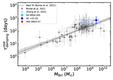
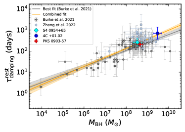
Figure 9: The damping timescale in the rest frame as a function of black hole mass. In both panels, the data points, line, and area in grey color represent the optical results from Burke et al. (2021). The light steel blue colored data points represent the $\gamma$-ray results from Zhang et al. (2022). The cyan, blue, and red data points are the results of our $\gamma$-ray analysis, corresponding to S4 0954+65, 4C +01.02, and PKS 0903-57, respectively. In the right panel, an orange line represents a combined fit to results from our study sample, Burke et al. (2021), and Zhang et al. (2022).

3.4 Flux distribution study

The flux distribution study helps us to understand the nature and origin of variability in the flux. A log-normal flux distribution has been observed in numerous blazars, manifesting at various wavelengths and timescales (H.E.S.S. Collaboration et al. 2010, Kushwaha et al. 2017, Shah et al. 2018, Sinha et al. 2018, Khatoon et al. 2019). In the case of AGN and X-ray binaries, it is well established that the multiplicative process in the disc produces the log-normal flux distribution (Uttley & McHardy, 2001). If it is believed that the disc and jet in the blazar are somehow connected then the fluctuations produced in the disc can travel to the jet and produce the disc-induced variability imprinting the log-normal flux distribution. In Biteau & Giebels (2012), they argue that the log-normal flux distribution can be produced by the minijets-in-a-jet statistical model, where the total flux is combined flux from many mini-jets which led to a skewed distribution. Their study also demonstrated that multiplicative processes can account for the log-normal flux distribution. Nevertheless, as indicated by Scargle (2020), the presence of a log-normal distribution in observed flux values does not necessarily imply the involvement of a multiplicative process.

Source	Flux (Normal)		Flux (Log-normal)
	AD statistic	p-value	AD statistic	p-value
4C +01.02	54.808	$<2.2\times 10^{-16}$	3.848	$1.34\times 10^{-9}$
PKS 0903-57	69.792	$<2.2\times 10^{-16}$	10.671	$<2.2\times 10^{-16}$
S4 0954+65	39.281	$<2.2\times 10^{-16}$	4.8	$6.558\times 10^{-12}$

Table 4: The AD statistic and corresponding p-values for the three sources. The null hypothesis of normal distribution is tested for flux and log-flux distributions.

3.4.1 Anderson-Darling test

The Anderson-Darling (AD) test is a statistical method for evaluating the null hypothesis concerning the data following a Gaussian distribution. The null hypothesis probability value, p-value holds that when p-value > 0.05, it supports the data would indicate Gaussian distribution. Conversely, if the p-value is below 0.05, it indicates a departure from the Gaussian distribution.

In order to achieve the light curves with good statistics, the flux points with a TS value greater than 9 (i.e. TS $>$ 9) were selected. Additionally, we refined the light curves by applying the condition that the ratio of the flux to its corresponding error ($f_{i}/\sigma_{i}>2$) must exceed 2 for each individual data point. The results of the AD test for both linear-scaled and logarithmic-scaled flux data are shown in Table 4. The outcomes of the test statistic suggest that the flux distribution for the sources 4C +01.02, PKS 0903-57, and S4 0954+65 does not support either a normal or lognormal distribution. We note that the AD statistic values for the log-normal case are an order of magnitude smaller compared to the normal case. We explore this further in the following section.

3.4.2 Log-flux histogram

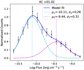
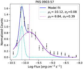
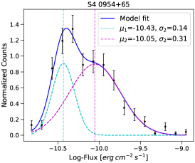
Figure 10: The figure shows double log-normal fits of the $\gamma$-ray flux histogram for the sources 4C +01.02, PKS 0903-57, and S4 0954+65 (left to right). For each plot above, the solid blue line represents the double log-normal fit. The two scaled components with factors $a$ and $(1-a)$ of equation 20 are shown as cyan and magenta dashed curves respectively. The vertical dashed lines are at $\mu_{1}$ and $\mu_{2}$ positions. The corresponding parameters for fit are shown in table 5.

We generate the normalized histogram of the logarithmic flux values for the three selected sources. The flux values are grouped into bins using the Freedman-Diaconis (FD) rule. The bin width of the histogram is decided such that it is greater than the average flux error of the data points within that bin (Shah et al., 2018). The flux histogram for the sources shows a double-peaked structure. Therefore, the log-flux histogram is fitted using the double Gaussian probability density functions (PDF) given by

$$f(x)=\frac{a}{\sqrt{2\pi}\sigma_{1}}\exp{\frac{-(x-\mu_{1})^{2}}{2\sigma_{1}^{2}}}+\frac{(1-a)}{\sqrt{2\pi}\sigma_{2}}\exp{\frac{-(x-\mu_{2})^{2}}{2\sigma_{2}^{2}}}$$ (20)

where $\mu_{1}$ and $\mu_{2}$ are mean values of the two Gaussian functions and $\sigma_{1}$ and $\sigma_{2}$ are their corresponding standard deviations. The functions are multiplied by scaling factors $a$ and $1-a$. The fits are shown in Figure 10 and the best-fit parameters are reported in Table 5. The reduced-$\chi^{2}$ statistic is used to estimate the quality of the fit.

Furthermore, we investigate the double-peaked histogram with the other combinations of distribution functions such as double Gaussian, a combination of single Gaussian and log-normal, and double log-normal. However, the obtained reduced-$\chi^{2}$ values exhibited less favorable results as compared to the double log-normal fits presented in Table 5 . The vertical lines in Figure 10 representing $\mu_{1}$ and $\mu_{2}$ are closer in the case of PKS 0903-57 (middle panel) compared to the other two sources and the standard deviation parameter $\sigma_{2}$ is much higher than $\sigma_{1}$ which is consistent with the data. The scaling factor $a$ is 0.20 which means the right component (dashed magenta curve) is dominant resulting in a lower profile of the left component (dashed cyan curve). The case of S4 0954+65 is similar. However, for 4C +01.02 the left component is dominant with a value 0.70. As we mentioned earlier for flux distribution study we choose the data points which have TS $>$ 9 which by default removes the upper limits. We tested the flux distribution by including the upper limits as well but it did not alter the existing shape of the distribution.

Source	$\mu_{1}$	$\mu_{2}$	$\sigma_{1}$	$\sigma_{2}$	$a$	DoF	$\chi^{2}/DoF$
4C +01.02	-10.11	-9.44	0.28	0.31	0.70	14	0.57
PKS 0903-57	-10.12	-9.84	0.08	0.39	0.20	17	3.46
S4 0954+65	-10.43	-10.05	0.14	0.31	0.31	15	1.86

Table 5: Results of the double Gaussian fit on the log-flux data for the three sources.

4 DISCUSSION

We present a comprehensive investigation aimed at characterizing the $\gamma$-ray variability exhibited by some selected Fermi blazars. Employing various approaches and methodologies, we analyze the light curves to elucidate the essence of $\gamma$-ray emissions and to understand the interplay between the accretion disc and relativistic jets.

From the analysis of fractional variability, as illustrated in Figure 4 and summarized in Table 1, for S4 0954+65, the UV and $\gamma$-ray emissions exhibit higher variability compared to its optical and X-ray emissions. In addition, a dip in the X-ray band resulted in a double-hump feature in the Fvar distribution. In the cases of PKS 0903-57 and 4C +01.02, the $\gamma$-ray emissions display a higher level of variability in comparison with the optical/UV and X-ray emissions. Specifically, for PKS 0903-57, an increment in $\gamma$-ray variability is approximately fourfold when compared to the UV band (see middle panel of Figure 4), while for 4C +01.02, it increases by a factor of $\sim$2.5 (see right panel of Figure 4).

A similar variability pattern has been reported in other blazars Abdo et al. (2011); Rani et al. (2016); Shah et al. (2021); Malik et al. (2022); Prince et al. (2022) as well. In the case of S4 0954+65, the observed distinctive pattern in Fvar distribution suggests that optical/UV and $\gamma$-ray emissions are associated with the synchrotron and inverse Compton (IC) processes involving high-energy electrons. On the other hand, the X-ray emission is linked to the IC process involving the lower-energy tail of the electron distribution. This observed variability can be attributed to relativistic electron cooling, wherein higher-energy electrons undergo more rapid cooling compared to their lower-energy counterparts. As a result, we observe higher variability in the emissions originating from high-energy electrons.

The PSD in AGN is well fitted with a single power law of form $P(\nu)\propto\nu^{-\beta}$, where the slope value spans the interval from 0 to 2 (Sobolewska et al., 2014). A case study focusing on a sample of blazars with $\gamma$-ray observations was conducted by (Bhatta & Dhital, 2020). The results of their investigation revealed that the slope index spans a range from 0.8 to 1.5. When $\beta$ equals 1, it is commonly referred to as long-term flicker noise, which can appear coherent for extended timescales (spanning decades). Our investigation involves fitting PSDs for all three sources using both single power law and bending power-law models. The obtained index values for the single power-law model are 0.80, 1.28, and 1.32 for S40954+65, PKS0903-57, and 4C+01.02, respectively. In addition, we observed breaks in frequency at 0.0047 (day^-1) for S4 0954+65, 0.004 (day^-1) for PKS 0903-57, and 0.0014 (day^-1) for 4C +01.02. The frequency break in PSD deduced from the DRW modeling is consistent within the error bar with the PSD break obtained from the observed data. In the case of 4C +01.02, the estimated PSD break from the data is not consistent with the DRW modeling suggesting the length of the light curve is not sufficient to derive a true PSD shape. Notably, the observed emissions are Doppler-boosted from the jets. The observed break frequency could potentially signify the impact of accretion disc events on the jets, driven through various mechanisms like accretion rates, magnetic fields, viscosity, and disc instabilities. These dynamic events might serve as drivers of jet emission variability. We compare the break time scale of PKS 0903-57 with the viscous time scale in the accretion disc and the timescale was found to be consistent suggesting a possible disc-jet coupling in the source.

Several authors have carried out an extensive investigation to explore the characteristic timescale of optical variability of AGN accretion disc (Collier & Peterson, 2001; Kelly et al., 2009; MacLeod et al., 2010; Simm et al., 2016; Suberlak et al., 2021). Additionally, Ryan et al. (2019); Zhang et al. (2022) extended these methodologies to investigate $\gamma$-ray variability within blazar samples.

Zhang et al. (2022) used the $\sim$12.7 years of $\gamma$-ray light curve of a sample of 23 AGN and modeled the variability with the stochastically driven damped simple harmonic oscillator (SHO) and the damped random-walk (DRW) models. In most of their cases, they find DRW explains the variability better than the SHO model. From the DRW modeling, they derived the damped random time scale which corresponds to the frequency break in the PSD, and plot it against the black hole mass. Their $\gamma$-ray sources almost occupy the same space in the $\tau^{rest}_{damping}$ – M_BH plot as the optical light curve derived for AGN in Burke et al. (2021), and they conclude that the observed break or DRW time scale in $\gamma$-ray corresponds to the processes in the accretion disc, suggesting a possible disc-jet coupling. Later, Zhang et al. (2023) used the broadband light curve from radio to $\gamma$-ray and modeled the variability with the DRW process. Their results suggest that the non-thermal optical, X-ray, and $\gamma$-ray are produced at the same location and radio at a farther distance. The derived time scale for non-thermal optical and $\gamma$-ray emission occupies the same space as thermal emission from the disc, suggesting the possible disc-jet coupling.

The derived damped random time scale for our three sources is also plotted on $\tau^{rest}_{damping}$ – M_BH space along with thermal time scale from Burke et al. (2021) and non-thermal time scale from Zhang et al. (2023). The plots are shown in Figure 9. First, we plot our three sources along with the disc time scale derived for AGN from Burke et al. (2021), we noticed that our sources exactly lying on the best-fit relation derived by Burke et al. (2021), suggesting the non-thermal $\gamma$-ray time scale in our three sources matching with thermal optical time scale derived for AGN. This led to the conclusion that the variability in the $\gamma$-ray light curve is linked with disc variability proving a possible disc-jet coupling. The non-thermal time scale derived for our three sources are also matching with the non-thermal time scale from Zhang et al. (2022) as shown in Figure 9. We fitted all the sources together to derive a combined standard relation for $\tau^{rest}_{damping}$ – M_BH and the slope is consistent within the error bar with Burke et al. (2021) and Zhang et al. (2022).

To perform the $\gamma$-ray flux distribution study, we use weekly binned Fermi-LAT light curve. The light curve was analyzed by the Anderson-Darling test. The test for normality of both the flux and log-flux was rejected due to the low p-values. The normalized log-flux distribution was further analyzed by fitting a double normal distribution function (see equation 20) owing to its double-peaked structure histogram, suggesting the presence of two distinct flux states. The fits for sources 4C +01.02 and PKS 0903-57 have $reduced-\chi^{2}$ values close to 1. Alternative combinations of normal and log-normal distribution functions were also investigated. However, it was observed that the most suitable choice for all three sources remained the double log-normal distribution. This conclusion holds even though the $reduced-\chi^{2}$ values range from 0.57 to 3.46 (see table 5).

As the X-ray binaries study suggests the variability produced in the accretion disc is caused by multiplicative processes which led to a log-normal flux distribution (Uttley & McHardy, 2001; Uttley et al., 2005). Our study shows that there is some connection between variability produced in the jet with the accretion disc. Therefore, we also produced the flux distribution of the $\gamma$-ray light curve for our sources. To mitigate bias in the flux distribution resulting from the possible lack of lower luminosity flux states, we have removed the flux with larger uncertainty, where $f_{i}/\sigma_{i}<2$. We noticed that the distribution rather follows a double log-normal flux distribution. In the investigation of multi-wavelength flux distribution in PKS 1510-089, Kushwaha et al. (2017) discovered two distinct log-normal profiles within the flux distribution at near-infrared (NIR), optical, and ${\gamma}$-ray wavelengths, which are associated with two possible flux conditions in the source. In a separate study by Khatoon et al. (2019), a dual Gaussian flux distribution was observed in the X-ray energy band for Mkn 501 and Mkn 421, providing additional support for the hypothesis of two distinct flux states. The origin of the double log-normal distribution is still unknown and the study done by Stecker & Salamon (1996); Stecker & Venters (2011) and Kushwaha et al. (2017) suggests it could be coming from the extragalactic $\gamma$-ray background.

5 Conclusion

In this study, we delved into several facets of multi-waveband variability exhibited by three distinct blazars, employing a range of methodologies. We emphasized our interest in characterizing the $\gamma$-ray variability. The findings of our investigation lead us to the following conclusions:

• We performed a comprehensive study involving fractional variability analysis using broadband light curves for three sources. Notably, in one of the sources, the observed variability pattern resembles a double-hump profile, as generally seen in broadband spectral energy distribution (SED) in blazars.

• To comprehensively study the statistical characteristics of the variability within $\gamma$-ray light curves over a wide range of temporal frequencies, we performed PSD analysis with extensive MC simulations. This study revealed a break in the $\gamma$-ray PSD for two sources. These observed break frequencies were subsequently confirmed through DRW modeling applied to $\gamma$-ray light curves. The observed PSD break time scale for PKS 0903-57 is consistent with the estimated viscous time scale in the accretion disk suggesting a possible scenario of disk-jet coupling.

• Analyzing the flux distribution, the presence of a log-normal distribution in blazar flux might indicate the involvement of multiplicative processes. These processes could involve perturbations in both the disk and/or the jet. The observed flux distribution in all three sources is accurately described by a double log-normal distribution, which has also been identified in earlier studies. This finding points to a complex scenario where underlying flaring activity emerges as a result of the combined variability of long and short timescales.

• The non-thermal damping time scale derived from the DRW modeling is consistent with the thermal damping time scale derived for optical AGN suggesting a possible disk-jet coupling in these three blazars. This serves as a motivation for studying a larger sample including broadband light curves to derive a fair conclusion.

Data Availability

This research has used $\gamma$-ray observations from Fermi-LAT and it can be accessed from publicly available LAT database server at https://fermi.gsfc.nasa.gov/ssc/data/access/. Additionally, this study also used data available in the X-ray and UVOT wavebands from the Neil Gehrels Swift Observatory and can be accessed from https://heasarc.gsfc.nasa.gov/w3browse/swift/swiftmastr.html.

References

- Abdo et al. (2010) Abdo A., et al., 2010, The Astrophysical Journal, 722, 520
- Abdo et al. (2011) Abdo A. A., et al., 2011, The Astrophysical Journal, 736, 131
- Ahnen et al. (2018) Ahnen M. L., et al., 2018, Astronomy & Astrophysics, 617, A30
- Aleksić et al. (2015a) Aleksić J., Ansoldi S., Antonelli L. A., Antoranz P., Babic A., Bangale 2015a, A&A, 576, A126
- Aleksić et al. (2015b) Aleksić J., Ansoldi S., Antonelli L. A., Antoranz P., Babic A., Bangale 2015b, A&A, 578, A22
- Bhatta & Dhital (2020) Bhatta G., Dhital N., 2020, The Astrophysical Journal, 891, 120
- Bhatta & Webb (2018) Bhatta G., Webb J. R., 2018, Galaxies, 6, x
- Bhattacharyya et al. (2020) Bhattacharyya S., Ghosh R., Chatterjee R., Das N., 2020, The Astrophysical Journal, 897, 25
- Biteau & Giebels (2012) Biteau J., Giebels B., 2012, A&A, 548, A123
- Breeveld et al. (2011) Breeveld A., Landsman W., Holland S., Roming P., Kuin N., Page M., 2011, in AIP Conference Proceedings. pp 373–376
- Brockwell (2001) Brockwell P. J., 2001, Handbook of statistics, 19, 249
- Brockwell & Davis (2002) Brockwell P. J., Davis R. A., 2002, Introduction to time series and forecasting. Springer
- Burke et al. (2021) Burke C. J., et al., 2021, Science, 373, 789
- Burrows et al. (2005) Burrows D. N., et al., 2005, Space Sci. Rev., 120, 165
- Camenzind & Krockenberger (1992) Camenzind M., Krockenberger M., 1992, Astronomy and Astrophysics (ISSN 0004-6361), vol. 255, no. 1-2, p. 59-62., 255, 59
- Chatterjee et al. (2008) Chatterjee R., et al., 2008, The Astrophysical Journal, 689, 79
- Chatterjee et al. (2018) Chatterjee R., Roychowdhury A., Chandra S., Sinha A., 2018, The Astrophysical Journal Letters, 859, L21
- Chen (2018) Chen L., 2018, The Astrophysical Journal Supplement Series, 235, 39
- Chen et al. (2016) Chen X., Pohl M., Böttcher M., Gao S., 2016, Monthly Notices of the Royal Astronomical Society, 458, 3260
- Collier & Peterson (2001) Collier S., Peterson B. M., 2001, The Astrophysical Journal, 555, 775
- Covino et al. (2020) Covino S., Landoni M., Sandrinelli A., Treves A., 2020, The Astrophysical Journal, 895, 122
- Edelson et al. (2002) Edelson R., Turner T., Pounds K., Vaughan S., Markowitz A., Marshall H., Dobbie P., Warwick R., 2002, The Astrophysical Journal, 568, 610
- Emmanoulopoulos et al. (2013) Emmanoulopoulos D., McHardy I., Papadakis I., 2013, Monthly Notices of the Royal Astronomical Society, 433, 907
- Fan & Cao (2004) Fan Z.-H., Cao X., 2004, The Astrophysical Journal, 602, 103
- Finke & Becker (2014) Finke J. D., Becker P. A., 2014, The Astrophysical Journal, 791, 21
- Foreman-Mackey et al. (2017) Foreman-Mackey D., Agol E., Ambikasaran S., Angus R., 2017, The Astronomical Journal, 154, 220
- Ghisellini & Tavecchio (2015) Ghisellini G., Tavecchio F., 2015, Monthly Notices of the Royal Astronomical Society, 448, 1060
- Giommi et al. (2006) Giommi P., et al., 2006, Astronomy & Astrophysics, 456, 911
- Goyal (2020) Goyal A., 2020, Monthly Notices of the Royal Astronomical Society, 494, 3432
- Goyal (2021) Goyal A., 2021, The Astrophysical Journal, 909, 39
- Goyal et al. (2017) Goyal A., et al., 2017, The Astrophysical Journal, 837, 127
- Goyal et al. (2018) Goyal A., et al., 2018, The Astrophysical Journal, 863, 175
- Goyal et al. (2022) Goyal A., et al., 2022, The Astrophysical Journal, 927, 214
- H.E.S.S. Collaboration et al. (2010) H.E.S.S. Collaboration et al., 2010, A&A, 520, A83
- Hewett et al. (1995) Hewett P. C., Foltz C. B., Chaffee F. H., 1995, Astronomical Journal (ISSN 0004-6256), vol. 109, no. 4, p. 1498-1521, 109, 1498
- Isobe et al. (2014) Isobe N., et al., 2014, The Astrophysical Journal, 798, 27
- Kasliwal et al. (2017) Kasliwal V. P., Vogeley M. S., Richards G. T., 2017, Monthly Notices of the Royal Astronomical Society, 470, 3027
- Kastendieck et al. (2011) Kastendieck M. A., Ashley M. C., Horns D., 2011, Astronomy & Astrophysics, 531, A123
- Kataoka et al. (2001) Kataoka J., et al., 2001, The Astrophysical Journal, 560, 659
- Kelly et al. (2009) Kelly B. C., Bechtold J., Siemiginowska A., 2009, The Astrophysical Journal, 698, 895
- Kelly et al. (2014) Kelly B. C., Becker A. C., Sobolewska M., Siemiginowska A., Uttley P., 2014, The Astrophysical Journal, 788, 33
- Khatoon et al. (2019) Khatoon R., Shah Z., Misra R., Gogoi R., 2019, Monthly Notices of the Royal Astronomical Society, 491, 1934
- Kozłowski (2017) Kozłowski S., 2017, Astronomy & Astrophysics, 597, A128
- Kozłowski et al. (2009) Kozłowski S., et al., 2009, The Astrophysical Journal, 708, 927
- Kushwaha et al. (2017) Kushwaha P., Sinha A., Misra R., Singh K., Dal Pino E. d. G., 2017, The Astrophysical Journal, 849, 138
- Lawrence et al. (1986) Lawrence C., Pearson T., Readhead A., Unwin S., 1986, The Astronomical Journal, 91, 494
- Lawrence et al. (1996) Lawrence C., Zucker J., Readhead A., Unwin S., Pearson T., Xu W., 1996, The Astrophysical Journal Supplement Series, 107, 541
- Li & Wang (2018) Li Y.-R., Wang J.-M., 2018, Monthly Notices of the Royal Astronomical Society: Letters, 476, L55
- Liodakis et al. (2017) Liodakis I., et al., 2017, Monthly Notices of the Royal Astronomical Society, 466, 4625
- Lu et al. (2019) Lu K.-X., et al., 2019, The Astrophysical Journal, 877, 23
- MacLeod et al. (2010) MacLeod C. L., et al., 2010, The Astrophysical Journal, 721, 1014
- Malik et al. (2022) Malik Z., Shah Z., Sahayanathan S., Iqbal N., Manzoor A., 2022, Monthly Notices of the Royal Astronomical Society, 514, 4259
- Marscher (2013) Marscher A. P., 2013, The Astrophysical Journal, 780, 87
- Matthews & Sandage (1963) Matthews T. A., Sandage A. R., 1963, Astrophysical Journal, vol. 138, p. 30, 138, 30
- Max-Moerbeck et al. (2014) Max-Moerbeck W., Richards J., Hovatta T., Pavlidou V., Pearson T., Readhead A., 2014, Monthly Notices of the Royal Astronomical Society, 445, 437
- Meyer et al. (2019) Meyer M., Scargle J. D., Blandford R. D., 2019, The Astrophysical Journal, 877, 39
- Nandra et al. (1997) Nandra K., George I., Mushotzky R., Turner T., Yaqoob T., 1997, The Astrophysical Journal, 476, 70
- Nilsson et al. (2018) Nilsson K., et al., 2018, Astronomy & Astrophysics, 620, A185
- Park & Trippe (2017) Park J., Trippe S., 2017, The Astrophysical Journal, 834, 157
- Pei et al. (2020) Pei Z., Fan J., Yang J., Bastieri D., 2020, Publications of the Astronomical Society of Australia, 37, e043
- Poutanen et al. (2008) Poutanen J., Zdziarski A. A., Ibragimov A., 2008, Monthly Notices of the Royal Astronomical Society, 389, 1427
- Press (1978) Press W. H., 1978, Comments on Modern Physics, Part C-Comments on Astrophysics, vol. 7, no. 4, 1978, p. 103-119., 7, 103
- Prince et al. (2022) Prince R., Khatoon R., Majumdar P., Czerny B., Gupta N., 2022, Monthly Notices of the Royal Astronomical Society, 515, 2633
- Rakshit & Stalin (2017) Rakshit S., Stalin C., 2017, The Astrophysical Journal, 842, 96
- Rani et al. (2016) Rani B., Krichbaum T. P., Lee S.-S., Sokolovsky K., Kang S., Byun D.-Y., Mosunova D., Zensus J. A., 2016, Monthly Notices of the Royal Astronomical Society, 464, 418
- Roming et al. (2005) Roming P. W., et al., 2005, Space Science Reviews, 120, 95
- Ryan et al. (2019) Ryan J. L., Siemiginowska A., Sobolewska M., Grindlay J., 2019, The Astrophysical Journal, 885, 12
- Scargle (2020) Scargle J. D., 2020, ApJ, 895, 90
- Schlafly & Finkbeiner (2011) Schlafly E. F., Finkbeiner D. P., 2011, The Astrophysical Journal, 737, 103
- Schreiber & Schmitz (1996) Schreiber T., Schmitz A., 1996, Physical review letters, 77, 635
- Schulz & Mudelsee (2002) Schulz M., Mudelsee M., 2002, Computers & Geosciences, 28, 421
- Schutte et al. (2022) Schutte H. M., et al., 2022, The Astrophysical Journal, 925, 139
- Shah et al. (2018) Shah Z., Mankuzhiyil N., Sinha A., Misra R., Sahayanathan S., Iqbal N., 2018, Research in Astronomy and Astrophysics, 18, 141
- Shah et al. (2021) Shah Z., Jithesh V., Sahayanathan S., Iqbal N., 2021, Monthly Notices of the Royal Astronomical Society, 504, 416
- Simm et al. (2016) Simm T., Salvato M., Saglia R., Ponti G., Lanzuisi G., Trakhtenbrot B., Nandra K., Bender R., 2016, Astronomy & Astrophysics, 585, A129
- Sinha et al. (2018) Sinha A., Khatoon R., Misra R., Sahayanathan S., Mandal S., Gogoi R., Bhatt N., 2018, Monthly Notices of the Royal Astronomical Society: Letters, 480, L116
- Sobolewska et al. (2014) Sobolewska M. A., Siemiginowska A., Kelly B. C., Nalewajko K., 2014, The Astrophysical Journal, 786, 143
- Stecker & Salamon (1996) Stecker F. W., Salamon M. H., 1996, ApJ, 464, 600
- Stecker & Venters (2011) Stecker F. W., Venters T. M., 2011, The Astrophysical Journal, 736, 40
- Stickel et al. (1993) Stickel M., Fried J., Kühr H., 1993, Astronomy and Astrophysics Supplement Series (ISSN 0365-0138), vol. 98, no. 3, p. 393-442., 98, 393
- Suberlak et al. (2021) Suberlak K. L., Ivezić Ž., MacLeod C., 2021, The Astrophysical Journal, 907, 96
- Tarnopolski et al. (2020) Tarnopolski M., Żywucka N., Marchenko V., Pascual-Granado J., 2020, The Astrophysical Journal Supplement Series, 250, 1
- Thompson et al. (1990) Thompson D., Djorgovski S., De Carvalho R., 1990, Publications of the Astronomical Society of the Pacific, 102, 1235
- Timmer & Koenig (1995) Timmer J., Koenig M., 1995, Astronomy and Astrophysics, 300, 707
- Ulrich et al. (1997) Ulrich M.-H., Maraschi L., Urry C. M., 1997, Annual Review of Astronomy and Astrophysics, 35, 445
- Urry & Padovani (1995) Urry C. M., Padovani P., 1995, Publications of the Astronomical Society of the Pacific, 107, 803
- Uttley & McHardy (2001) Uttley P., McHardy I. M., 2001, Monthly Notices of the Royal Astronomical Society, 323, L26
- Uttley et al. (2002) Uttley P., McHardy I., Papadakis I., 2002, Monthly Notices of the Royal Astronomical Society, 332, 231
- Uttley et al. (2005) Uttley P., McHardy I. M., Vaughan S., 2005, Monthly Notices of the Royal Astronomical Society, 359, 345
- Vaughan et al. (2003) Vaughan S., Edelson R., Warwick R., Uttley P., 2003, Monthly Notices of the Royal Astronomical Society, 345, 1271
- Wagner & Witzel (1995) Wagner S., Witzel A., 1995, Annual Review of Astronomy and Astrophysics, 33, 163
- Wiita (2006) Wiita P. J., 2006, in Miller H. R., Marshall K., Webb J. R., Aller M. F., eds, Astronomical Society of the Pacific Conference Series Vol. 350, Blazar Variability Workshop II: Entering the GLAST Era. p. 183 (arXiv:astro-ph/0507141), doi:10.48550/arXiv.astro-ph/0507141
- Wood et al. (2017) Wood M., Caputo R., Charles E., Di Mauro M., Magill J., Perkins J. S., Fermi-LAT Collaboration 2017, in 35th International Cosmic Ray Conference (ICRC2017). p. 824 (arXiv:1707.09551), doi:10.22323/1.301.0824
- Yang et al. (2021) Yang S., Yan D., Zhang P., Dai B., Zhang L., 2021, The Astrophysical Journal, 907, 105
- Zhang et al. (2020) Zhang L., Chen S., Xiao H., Cai J., Fan J., 2020, The Astrophysical Journal, 897, 10
- Zhang et al. (2022) Zhang H., Yan D., Zhang L., 2022, The Astrophysical Journal, 930, 157
- Zhang et al. (2023) Zhang H., Yan D., Zhang L., 2023, The Astrophysical Journal, 944, 103
- Zu et al. (2013) Zu Y., Kochanek C., Kozłowski S., Udalski A., 2013, The Astrophysical Journal, 765, 106