CoPriv: Network/Protocol Co-Optimization for Communication-Efficient Private Inference

Abstract

Deep neural network (DNN) inference based on secure 2-party computation (2PC) can offer cryptographically-secure privacy protection but suffers from orders of magnitude latency overhead due to enormous communication. Previous works heavily rely on a proxy metric of ReLU counts to approximate the communication overhead and focus on reducing the ReLUs to improve the communication efficiency. However, we observe these works achieve limited communication reduction for state-of-the-art (SOTA) 2PC protocols due to the ignorance of other linear and non-linear operations, which now contribute to the majority of communication. In this work, we present CoPriv, a framework that jointly optimizes the 2PC inference protocol and the DNN architecture. CoPriv features a new 2PC protocol for convolution based on Winograd transformation and develops DNN-aware optimization to significantly reduce the inference communication. CoPriv further develops a 2PC-aware network optimization algorithm that is compatible with the proposed protocol and simultaneously reduces the communication for all the linear and non-linear operations. We compare CoPriv with the SOTA 2PC protocol, CrypTFlow2, and demonstrate 2.1$\times$ communication reduction for both ResNet-18 and ResNet-32 on CIFAR-100. We also compare CoPriv with SOTA network optimization methods, including SNL, MetaPruning, etc. CoPriv achieves 9.98$\times$ and 3.88$\times$ online and total communication reduction with a higher accuracy compared to SNL, respectively. CoPriv also achieves 3.87$\times$ online communication reduction with more than 3% higher accuracy compared to MetaPruning.

1 Introduction

Deep learning has been applied to increasingly sensitive and private data and tasks, for which privacy emerges as one of the major concerns. To alleviate the privacy concerns when deploying the deep neural network (DNN) models, secure two-party computation (2PC) based DNN inference is proposed and enables cryptographically-strong privacy guarantee mohassel2017secureml ; juvekar2018gazelle ; srinivasan2019delphi ; reagen2021cheetah ; hussain2021coinn ; huang2022cheetah ; shen2022abnn2 .

Secure 2PC helps solve the following dilemma juvekar2018gazelle ; srinivasan2019delphi ; reagen2021cheetah : the server owns a private model and the client owns private data. The server is willing to provide the machine learning as a service (MLaaS) but does not want to give it out directly. The client wants to apply the model on the private data without revealing it as well. Secure 2PC frameworks can fulfill both parties’ requirements: two parties can learn the inference results but nothing else beyond what can be derived from the results.

The privacy protection of secure 2PC-based inference is achieved at the cost of high communication complexity due to the massive interaction between the server and the client kumar2020cryptflow ; srinivasan2019delphi ; rathee2020cryptflow2 ; hussain2021coinn . This leads to orders of magnitude latency gap compared to the regular inference on plaintext kumar2020cryptflow ; rathee2020cryptflow2 . A 2PC-based inference usually has two stages, including a pre-processing stage that generates the input independent helper data and an online stage to process client’s actual query kumar2020cryptflow ; srinivasan2019delphi ; rathee2020cryptflow2 ; hussain2021coinn ; huang2022cheetah . Because the helper data is independent of client’s query, previous works srinivasan2019delphi ; hussain2021coinn assume the pre-processing stage is offline and thus, focus on optimizing the communication of the input dependent stage. Specifically, srinivasan2019delphi ; ghodsi2020cryptonas ; jha2021deepreduce ; cho2022sphynx ; cho2022selective ; kundu2023learning observe ReLU accounts for significant communication and ReLU count is widely used as a proxy metric for the inference efficiency. Hence, the problem of improving inference efficiency is usually formulated as optimizing networks to have as few ReLUs as possible. For example, DeepReduce jha2021deepreduce and SNL cho2022selective achieve more than 4$\times$ and 16$\times$ ReLU reduction with less than 5% accuracy degradation on the CIFAR-10 dataset.

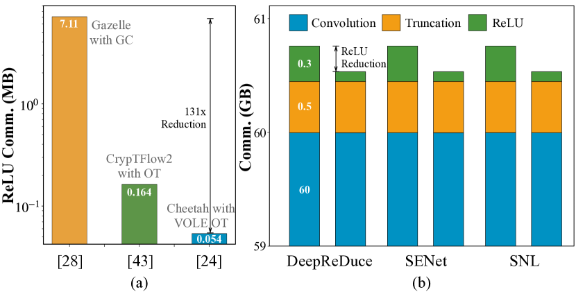
Figure 1: (a) Communication for ReLU communication has reduced by 131$\times$ from juvekar2018gazelle to huang2022cheetah ; (b) existing network optimizations suffers from limited reduction of online and total communication.

However, such assumption may no longer be valid for state-of-the-art (SOTA) 2PC protocols. We profile the communication of ResNet-18 with different ReLU optimization algorithms, including DeepReduce jha2021deepreduce , SENet kundu2023learning , and SNL cho2022selective and observe very limited communication reduction as shown in Figure 1(b). This is because, on one hand, the communication efficiency of ReLU has been drastically improved over the past few years from garble circuit (GC) to VOLE oblivious transfer (OT) as shown in Figure 1(a) juvekar2018gazelle ; rathee2020cryptflow2 ; huang2022cheetah , and ReLU only accounts for 40% and 1% of the online and total communication, respectively. On the other hand, recent studies suggest for MLaaS, it is more important to consider inference request arrival rates rather than studying individual inference in isolation garimella2023characterizing . In this case, the pre-processing communication, which is significantly higher than the online communication as shown in Figure 1(b), cannot be ignored and may often be incurred online as there may not be sufficient downtime for the server to hide its latency garimella2023characterizing .

Therefore, to improve the efficiency of 2PC-based inference, in this paper, we argue that both pre-processing and online communication are important and propose CoPriv to jointly optimize the 2PC protocol and the DNN architecture. CoPriv first optimizes the inference protocol for the widely used 3-by-3 convolutions based on the Winograd transformation and proposes a series of DNN-aware protocol optimization. The optimized protocol achieves more than 2.1$\times$ communication reduction for ResNet models he2016deep without accuracy impact. For lightweight mobile networks, e.g., MobileNetV2 sandler2018mobilenetv2 , we propose a differentiable ReLU pruning and re-parameterization algorithm in CoPriv. Different from existing methods jha2021deepreduce ; cho2022selective ; kundu2023learning , CoPriv optimizes both linear and non-linear operations to simultaneously improve both the pre-processing and online communication efficiency.

With extensive experiments, we demonstrate CoPriv drastically reduces the communication of 2PC-based inference. The proposed optimized protocol with Winograd transformation reduces the convolution communication by 2.1$\times$ compared to prior-art CrypTFlow2 rathee2020cryptflow2 for both the baseline ResNet models. With joint protocol and network co-optimization, CoPriv outperforms SOTA ReLU-optimized methods and pruning methods. Our study motivates the community to directly use the communication as the efficiency metric to guide the protocol and network optimization.

2 Preliminaries

2.1 Threat Model

CoPriv focuses on efficient private DNN inference involving two parites, i.e., Alice (server) and Bob (client). The server holds the model with private weights and the client holds private inputs. At the end of the protocol execution, the client learns the inference results without revealing any information to the server. Consistent with previous works mohassel2017secureml ; srinivasan2019delphi ; rathee2020cryptflow2 ; rathee2021sirnn ; jha2021deepreduce ; cho2022selective ; kundu2023learning , we adopt an honest-but-curious security model in which both parties follow the protocol but also try to learn more from the information than allowed. Meanwhile, following mohassel2017secureml ; juvekar2018gazelle ; srinivasan2019delphi ; rathee2020cryptflow2 ; rathee2021sirnn , we assume no trusted third party exists so that the helper data needs to be generated by the client and the server.

2.2 Arithmetic Secret Sharing

CoPriv leverages the 2PC framework based on arithmetic secret sharing (ArSS). Specifically, an $l$-bit value $x$ is shared additively in the integer ring $\mathbb{Z}_{2^{l}}$ as the sum of two values, e.g., $\langle x\rangle_{s}$ and $\langle x\rangle_{c}$. $x$ can be reconstructed as $\langle x\rangle_{s}+\langle x\rangle_{c}$ mod $2^{l}$. In the 2PC framework, $x$ is secretly shared with the server holding $\langle x\rangle_{s}$ and the client holding $\langle x\rangle_{c}$.

ArSS supports both addition and multiplication on the secret shares. Addition can be conducted locally while multiplication requires helper data, which are independent of the secret shares and is generated through communication rathee2020cryptflow2 ; rathee2021sirnn . The communication cost of a single multiplication of secret shares is $O(l(\lambda+l))$. When $t$ multiplications share the same multiplier, instead of simply repeating the multiplication protocol for $t$ times, demmler2015aby ; kumar2020cryptflow ; rathee2020cryptflow2 proposes a batch optimization algorithm that only requires $O(l(\lambda+tl))$ communication, enabling much more efficient batched multiplications.

Most 2PC frameworks use fixed-point arithmetic. The multiplication of two fixed-point values of $l$-bit precision results in a fixed-point value of $2l$-bit precision. Hence, in order to perform subsequent arithmetics, a truncation is required to scale the value down to $l$-bit precision. Truncation usually executes after the convolutions and before the ReLUs. It requires complex communication and sometimes leads to even more online communication compared to ReLU as shown in Figure 1. We refer interested readers to rathee2020cryptflow2 for more details.

2.3 Winograd Convolution

Table 1: Comparison with prior-art methods.

Method	Protocol Opt.	Network Opt.
		Conv.	Truncation	ReLU
rathee2020cryptflow2 ; rathee2021sirnn ; mohassel2017secureml ; demmler2015aby ; mohassel2018aby3 ; knott2021crypten ; rathee2022secfloat	✓	✗	✗	✗
kundu2023learning ; cho2022selective ; ghodsi2020cryptonas ; peng2022polympcnet ; lou2021safenet ; cho2022sphynx ; jha2023deepreshape ; jha2021deepreduce	✗	✗	✗	✓
srinivasan2019delphi ; hussain2021coinn	✓	✗	✗	✓
ganesan2022efficient	✓	✓	✗	✗
CoPriv (ours)	✓	✓	✓	✓

Table 2: Notations used in the paper.

Notation	Meaning
$H,W$	Height and width of output feature map
$C,K$	Input and output channel number
$A,B,G$	Winograd transformation matrices
$m,r$	Size of output tile and convolution filter
$T$	Number of tiles per input channel
$\lambda$	Security parameter that measures the attack hardness

We first summarize all the notations used in the paper in Table 2. Then, consider a 1D convolution with $m$ outputs and filter size of $r$, denoted as $F(m,r)$. With regular convolution, $F(m,r)$ requires $mr$ multiplications between the input and the filter. With the Winograd algorithm, $F(m,r)$ can be computed differently. Consider the example of $F(2,3)$ below:

$$X=\begin{bmatrix}x_{0}&x_{1}&x_{2}&x_{4}\end{bmatrix}^{\top}\quad W=\begin{bmatrix}w_{0}&w_{1}&w_{2}\end{bmatrix}^{\top}\quad Y=\begin{bmatrix}y_{0}&y_{1}\end{bmatrix}^{\top}$$

$$\begin{bmatrix}x_{0}&x_{1}&x_{2}\\ x_{1}&x_{2}&x_{3}\end{bmatrix}\begin{bmatrix}w_{0}\\ w_{1}\\ w_{2}\end{bmatrix} =\begin{bmatrix}m_{0}+m_{1}+m_{2}\\ m_{1}-m_{2}-m_{3}\end{bmatrix}=\begin{bmatrix}y_{0}\\ y_{1}\end{bmatrix}$$

where $m_{0},m_{1},m_{2},m_{3}$ are computed as

$$\begin{matrix}m_{0}=(x_{0}-x_{2})w_{0}&m_{1}=(x_{1}+x_{2})(w_{0}+w_{1}+w_{2})/2\\ m_{3}=(x_{1}-x_{3})w_{2}&m_{2}=(x_{2}-x_{1})(w_{0}-w_{1}+w_{2})/2\end{matrix}.$$

With the Winograd algorithm, the number of multiplications is reduced from 6 in the regular convolution to 4. Similar Winograd transformation can be applied to 2D convolutions by nesting 1D algorithm with itself lavin2016fast . The 2D Winograd transformation $F(m\times m,r\times r)$, where the output tile size is $m\times m$, the filter size is $r\times r$, and the input tile size is $n\times n$, where $n=m+r-1$, can be formulated as follows,

$$Y=W\circledast X=A^{\top}[(GWG^{\top})\odot(B^{\top}XB)]A,$$ (1)

where $\circledast$ denotes the regular convolution and $\odot$ denotes element-wise matrix multiplication (EWMM). $A$, $B$, and $G$ are transformation matrices that are independent of $W$ and $X$ and can be computed based on $m$ and $r$ lavin2016fast ; alam2022winograd .

With the Winograd algorithm, the multiplication of such a 2D convolution can be reduced from $m^{2}r^{2}$ to $n^{2}$, i.e., $(m+r-1)^{2}$ at the cost of performing more additions which can be computed locally in private inference scenario. While the reduction of multiplication increases with $m$, $m=2$ and $m=4$ are most widely used for the better inference precision lavin2016fast ; vincent2017improving ; barabasz2020error ; fernandez2020searching . More details about Winograd convolution are available in Appendix D.

2.4 Related Works

To improve the efficiency of private inference, existing works can be categorized into three classes, including protocol optimization demmler2015aby ; mohassel2018aby3 ; rathee2020cryptflow2 ; rathee2021sirnn ; knott2021crypten ; rathee2022secfloat ; mohassel2017secureml , network optimization jha2021deepreduce ; cho2022selective ; ghodsi2020cryptonas ; peng2022polympcnet ; lou2021safenet ; cho2022sphynx ; kundu2023learning ; jha2023deepreshape ; zeng2023mpcvit ; li2022mpcformer , and joint optimization srinivasan2019delphi ; hussain2021coinn ; ganesan2022efficient . In Table 2, we compare CoPriv with these works qualitatively and as can be observed, CoPriv leverages both protocol and network optimization and can simultaneously reduce the online and total communication induced by convolutions, truncations, and ReLUs through network optimization. We leave more detailed review of existing works to Appendix A and more detailed comparison in terms of their techniques to Appendix F.

3 Motivation

In this section, we analyze the origin of the limited communication reduction of existing ReLU-optimized networks and discuss our key observations that motivates CoPriv.

Observation 1: the total communication is dominated by convolutions while the online communication cost of truncations and ReLUs are comparable.

As shown in Figure 1, the main operations that incurs high communication costs are convolutions, truncations, and ReLUs. With CrypTFlow2, over 95% communication is in the pre-processing stage generated by convolutions, while the truncations and ReLUs requires similar communication. This observation contradicts to the assumption of previous works cho2022selective ; cho2022sphynx ; ghodsi2020cryptonas ; kundu2023learning : on one hand, ReLU no longer dominates the online communication and simply reducing ReLU counts leads to diminishing return for online communication reduction; on the other hand, pre-processing communication cannot be ignored as it not only consumes a lot of power in the server and client but also can slow down the online stage. As pointed out by a recent system analysis garimella2023characterizing , for a pratical server that accepts inference request under certain arrival rates, the pre-processing stage is often incurred online as there is insufficient downtime to hide its latency. Therefore, we argue that both the total and the online communication are crucial and need to be reduced to enable more practical 2PC-based inference.

Observation 2: the communication cost scaling of convolution, truncation and ReLU is different with the network dimensions.

The communication cost of different operations scales differently with the network dimensions. For a convolution, the major operations are multiplications and additions. While additions are computed fully locally, multiplications requires extra communication to generate the helper data. Hence, the communication cost for a convolution scales linearly with the number of multiplications and the complexity is $O(CKr^{2}(\lambda+HW))$ following hussain2021coinn . Both truncations and ReLUs are element-wise and hence, their communication cost scales linearly with the input feature size, i.e., $O(HWC)$. Therefore, for networks with a large number of channels, the pre-processing communication becomes even more dominating.

Since the communication is dominated by the multiplications in convolution layers, our intuition is to reduce the multiplications by conducting more local additions for better communication efficiency. Meanwhile, as in Figure 3, MobileNetV2 are much more communication efficient compared to ResNets with a similar accuracy, and hence, becomes the focus of our paper.

Figure 2: Comparison of communication breakdown between ResNet-50 and MobileNetV2 on ImageNet.

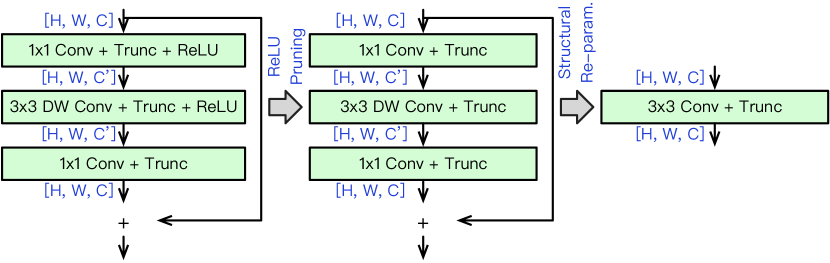
Figure 3: Illustration of ReLU pruning and network re-parameterization for communication reduction. DW means depth-wise and $1\times 1$ Conv is also called point-wise (PW) convolution.

Observation 3: ReLU pruning and network re-parameterization can simultaneously reduce the online and total communication of all operations.

Existing network optimizations either linearize the ReLUs selectively jha2021deepreduce ; cho2022selective ; peng2022polympcnet ; lou2021safenet ; cho2022sphynx ; kundu2023learning or prune the whole channel or layer liu2019metapruning . Selective ReLU linearization usually achieves a better accuracy but achieves limited communication reduction. In contrast, channel-wise or layer-wise pruning can simultaneously reduce the communication for all the operators but usually suffers from a larger accuracy degradation jha2021deepreduce . We observe for an inverted residual block in MobileNetV2, as shown in Figure 3, if both of the two ReLUs are removed, the block can be merged into a dense convolution after training. During training, this preserves the benefits of over-parameterization shown in RepVGG ding2021repvgg to protect network accuracy, while during inference, the dense convolution is more compatible with our optimized protocol and can reduce communication of truncations as well.

4 CoPriv: A New Paradigm Towards Efficient Private Inference

In this section, we present CoPriv, a protocol-network co-optimization framework for communication-efficient 2PC-based inference. The overview of CoPriv is shown in Figure 4. Given the original network, we first leverage the Winograd transformation with DNN-aware optimization to reduce the communication when computing 3-by-3 convolutions without any accuracy impact (Section 4.1). The optimized transformation enables to reduce the total communication of ResNet-18 by 2.1$\times$. However, the communication reduction of MobileNetV2 is limited as the Winograd transformation can only be applied to the 3-by-3 depth-wise convolution, which only contributes to a small portion of the total communication. Hence, for MobileNetV2, we propose an automatic and differentiable ReLU pruning algorithm (Section 4.2). By carefully designing the pruning pattern, CoPriv enables further network re-parameterization of the pruned networks, which reduces the online and total communication by 5$\times$ and 5$\times$ in the example, respectively, combining with our optimized convolution protocol.

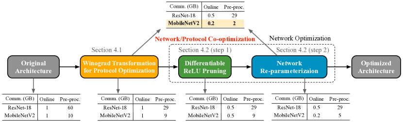
Figure 4: Overview of CoPriv and the communication cost after each optimization step. The example of the communication cost is measured on the CIFAR-100 dataset.

4.1 Winograd Transformation for Protocol Optimization

We propose to leverage the Winograd transformation to reduce the communication when computing a convolution. Following Eq. 1, for each 2D output tile, because $A,B,G$ are known publicly, the filter transformation $GWG^{\top}$ and feature transformation $B^{\top}XB$ can be computed locally on the server and client ganesan2022efficient . Then, EWMM is performed together by the server and the client through communication while the final output transformation $A^{\top}[\cdot]A$ can be computed locally as well.

For each output tile, as $(m+r-1)^{2}$ multiplications are needed and there is no shared multiplier for batch optimization described in Section 2.2, the communication cost is $O(\lambda(m+r-1)^{2})$ . Consider there are in total $T=\lceil H/m\rceil\times\lceil W/m\rceil$ tiles per output channel, $C$ input channels, and $K$ output channels, the communication complexity of a convolution layer now becomes $O(\lambda TCK(m+r-1)^{2})$. To reduce the enormous communication, we present the following optimizations.

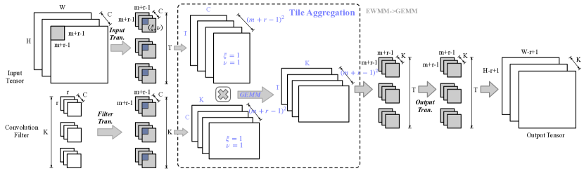
Figure 5: Winograd transformation procedure with tile aggregation.

Table 3: Communication complexity of different convolution types and the measured communication for a ResNet-18 block with 14$\times$14$\times$256 feature dimension.

Conv. Type	Comm. Complexity	ResNet Block Comm. (GB)
Regular Conv.	$O(CKr^{2}(\lambda+HW))$	23.74 (1$\times$)
EWMM-based Winograd Conv.	$O(\lambda CKT(m+r-1)^{2})$	256 (10.78$\times\uparrow$)
+ Tile Aggregation (GEMM-based)	$(m+r-1)^{2}CT(\lambda+K)$	10.45 (2.27$\times\downarrow$)
+ DNN-aware Sender Selection	$\mathrm{min}[(m+r-1)^{2}CT(\lambda+K),$ $(m+r-1)^{2}CK(\lambda+T)]$	7.76 (3.06$\times\downarrow$)

Communication reduction with tile aggregation

While the Winograd transformation helps to reduce the total number of multiplications, in Table 3, we observe the communication for a ResNet block actually increases. This is because the baseline protocol can leverage the batch optimization mentioned in Section 2.2 to reduce the communication complexity. To further optimize the Winograd-based convolution protocol to adapt to private inference, we observe the following opportunities for the batch optimization: first, each transformed input tile needs to multiply all the $K$ filters; secondly, each transformed filter needs to multiply all the transformed input tiles for a given channel. Hence, for the $t$-th tile in $f$-th output channel, we re-write Eq. 1 as follows:

$$Y_{f,t}=A^{\top}[\sum_{c=1}^{C}U_{f,c}\odot V_{c,t}]A\quad 1\leq f\leq K,1\leq t\leq T,$$

where $U_{f,c}$ denotes the transformed filter correspnding to the $f$-th output channel and $c$-th input channel and $V_{c,t}$ denotes the transformed input of the $t$-th tile in the $c$-th input channel. Then, consider each pixel location, denoted as $(\xi,\nu)$, within the tile separately, yielding:

$$Y^{(\xi,\nu)}_{f,t}=A^{\top}[U^{(\xi,\nu)}_{f,c}V^{(\xi,\nu)}_{c,t}]A\quad 1\leq f\leq K,1\leq t\leq T,1\leq\xi,\nu\leq m+r-1$$

We illustrate this transformation procedure in Figure 5. Re-writing the EWMM into general matrix multiplication (GEMM) enables us to fully leverage the batch optimization and reduce the communication complexity as shown in Table 3. We can now reduce the communication of a ResNet block by 2.27$\times$.

DNN-aware adaptive convolution protocol

When executing the convolution protocol, both the server and the client can initiate the protocol. Because the input feature map and the filter are of different dimensions, we observe the selection of protocol intializer impacts the communication round as well as the communication complexity. While CrypTFlow2 always selects the server to initialize the protocol, we propose DNN architecture-aware convolution protocol to choose between the server and the client adaptively based on the layer dimensions to minimize the communication complexity. As shown in Table 3, the communication of the example ResNet block can be further reduced by 1.35$\times$ with the adaptive protocol.

4.2 Differentiable ReLU Pruning and Network Re-Parameterization

We now describe our network optimization algorithm to further reduce both pre-processing and online communication for MobileNetV2. The core idea is to simultaneously remove the two ReLUs within an inverted residual block together, after which the entire block can be merged into a dense convolution layer to be further optimized with our Winograd-based protocol as in Figure 3. For the example in Figure 4, both the pre-processing and online communication for MobileNetV2 can be reduced by 5$\times$. To achieve the above goal, the remaining questions to answer include: 1) which ReLUs to remove and how to minimize the accuracy degradation for the pruned networks, and 2) how to re-parameterize the inverted residual block to guarantee functional correctness. Hence, we propose the following two-step algorithm.

Step 1: communication-aware differentiable ReLU pruning

To identify “unimportant” activation functions, CoPriv leverages a differentiable pruning algorithm. Specifically, CoPriv assigns an architecture parameter $\alpha(0\leq\alpha\leq 1)$ to measure the importance of each ReLU. During pruning, the forward function of a ReLU now becomes $\alpha\cdot\mathrm{ReLU}(x)+(1-\alpha)\cdot x$. CoPriv jointly learns the model weights $\theta$ and the architecture parameters $\alpha$. Specifically, given a sparsity constraint $s$, we propose the one-level optimization formulated as follows:

$$\min_{\theta,\alpha}\mathcal{L}_{CE}+\mathcal{L}_{comm}\quad\mathrm{s.t.}\quad||\alpha||_{0}\leq s,$$ (2)

where $\mathcal{L}_{CE}$ is the task-specific cross entropy loss and $\mathcal{L}_{comm}$ is the communication-aware regularization to focus the pruning on communication-heavy blocks and is defined as

$$\mathcal{L}_{comm}=\sum_{i}\alpha_{i}(\mathrm{Comm}_{i}(\alpha_{i}=1)-\mathrm{Comm}_{i}(\alpha_{i}=0)),$$

where $\mathrm{Comm}_{i}(\alpha_{i}=1)$ is the communication to compute the $i$-th layer when $\alpha_{i}=1$. We also show the effectiveness of communication-aware regularization in the experimental results. To ensure the network after ReLU pruning can be merged, two ReLUs within the same block share the same $\alpha$. During training, in the forward process, only the top-$s$ $\alpha$’s are activated (i.e., $\alpha=1$) while the remainings are set to 0. In the backpropagation process, $\alpha$’s are updated via straight-through estimation (STE) bengio2013estimating .

Once the pruning finishes, the least important ReLUs are removed and we perform further finetuning to improve the network accuracy. Specifically, in CoPriv, we leverage knowledge distillation (KD) hinton2015distilling to guide the finetuning of the pruned network.

Step 2: network re-parameterization

The removal of ReLUs makes the inverted residual block linear, and thus can be further merged together into a single dense convolution. Motivated by the previous work of structural re-parameterization fu2022depthshrinker ; ding2021repvgg ; ding2021diverse ; ding2019acnet ; ding2022repmlpnet ; ding2021resrep , we describe the detailed re-parameterization algorithm in Appendix C. The re-parameterized convolution has the same number of input and output channels as the first and last point-wise convolution, respectively. Its stride equals to the stride of the depth-wise convolution.

5 Experiments

5.1 Experimental Setup

We adopt CypTFlow2 rathee2020cryptflow2 protocol for the 2PC-based inference, and we measure the communication and latency under a LAN setting rathee2020cryptflow2 with 377 MBps bandwidth and 0.3ms echo latency. For Winograd, we implement $F(2\times 2,3\times 3)$ and $F(4\times 4,3\times 3)$ transformation for convolution with stride of 1 and $F(2\times 2,3\times 3)$ transformation when stride is 2 huang2021efficient . We apply CoPriv to MobileNetV2 with different width multipliers on CIFAR-100 krizhevsky2009learning and ImageNet deng2009imagenet datasets. The details of our experimental setups including the private inference framework, the implementation of the Winograd-based convolution protocol and the training details are available in Appendix B.

5.2 Micro-Benchmark on the Convolution Protocol with Winograd Transformation

We first benchmark the communication reduction of the proposed convolution protocol based on Winograd transformation. The results on ResNet-18 and ResNet-32 are shown in Figure 6(a) and (b). As can be observed, the proposed protocol consistently reduces the communication to compute the convolutions. While the degree of communication reduction depends on the layer dimensions, on average, 2.1$\times$ reduction is achieved for both ResNet-18 and ResNet-32. We also benchmark the Winograd-based protocol with output tile sizes of 2 and 4, i.e., $F(2\times 2,3\times 3)$ and $F(4\times 4,3\times 3)$. Figure 6(c) shows that when the feature resolution is small, a small tile size achieves more communication reduction while larger resolution prefers a larger tile size. Hence, for the downstream experiments, we use $F(2\times 2,3\times 3)$ for CIFAR-100 and $F(4\times 4,3\times 3)$ for ImageNet deng2009imagenet dataset, respectively.

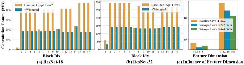
Figure 6: Communication of the convolution protocol with Winograd transformation on (a) ResNet-18 and (b) ResNet-32 on CIFAR-100; (c) comparison between $F(2\times 2,3\times 3)$ and $F(4\times 4,3\times 3)$ with different feature dimensions.

5.3 Benchmark with ReLU-Optimized Networks on CIFAR-100

We benchmark CoPriv with different network optimization algorithms that focus on reducing ReLU counts, including DeepReDuce jha2021deepreduce , SENet kundu2023learning and SNL cho2022selective , on the CIFAR-100 dataset. As DeepReDuce, SENet and SNL all use ResNet-18 as the baseline model, we also train SNL algorithm on the MobileNetV2-w0.75 for a comprehensive comparison.

Results and analysis

From Figure 7, we make the following observations: 1) previous methods, including DeepReDuce, SENet, SNL, do not reduce the pre-processing communication and their online communication reduction quickly saturates with a notable accuracy degradation; 2) CoPriv achieves SOTA Pareto front of accuracy and online/total communication. Specifically, CoPriv outperforms SNL on ResNet-18 with 4.3% higher accuracy as well as 1.55$\times$ and 19.5$\times$ online and total communication reduction, respectively. When compared with SNL on MobileNetV2-w0.75, CoPriv achieves 1.67% higher accuracy with 1.66$\times$ and 2.44$\times$ online and total communication reduction, respectively.

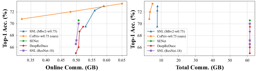
Figure 7: Comparison with efficient ReLU-optimized methods on CIFAR-100 dataset.

5.4 Benchmark on ImageNet

We also benchmark CoPriv on the ImageNet dataset with the following baselines: lightweight mobile networks like MobileNetV3 howard2019searching with different capacities, ReLU-optimized networks, including SNL cho2022selective and SENet kundu2023learning , and SOTA pruning methods, including uniform pruning and MetaPruning liu2019metapruning . We train both our CoPriv and SNL on the MobileNetV2-w1.4 with self distillation.

Results and analysis

From the results shown in Figure 8, we observe that 1) compared with SNL on MobileNetV2-w1.4, CoPriv achieves 1.4% higher accuracy with 9.98$\times$ and 3.88$\times$ online and total communication reduction, respectively; 2) CoPriv outperforms 1.8% higher accuracy compared with MobileNetV3-Small-1.0 while achieving 9.41$\times$ and 1.67$\times$ online and total communication reduction; 3) CoPriv demonstrates its strong scalability for communication optimization. Compared to the baseline MobileNetV2-w1.4, CoPriv achieves 2.52$\times$ and 1.9$\times$ online and total communication reduction, respectively without compromising the accuracy; 4) when compared with SOTA pruning methods, for a high communication budget, CoPriv-w1.4-B achieves 1.6% higher accuracy with 2.28$\times$ and 1.08$\times$ online and total communication reduction, compared with MetaPruning-1.0$\times$; for a low communication budget, compared with MetaPruning-0.35$\times$, CoPriv-w1.4-D achieves 5.5% higher accuracy with 3.87$\times$ online communication reduction.

Figure 8: Comparison with SOTA efficient ConvNets, ReLU-optimized methods, channel-wise pruning MetaPruning liu2019metapruning and uniform pruning on ImageNet dataset. We mark the four points of CoPriv as CoPriv-w1.4-A/B/C/D from left to right, respectively.

5.5 Ablation Study

Effectiveness of different optimizations in CoPriv

To understand how different optimizations help improve communication efficiency, we add our proposed protocol optimizations step by step on both SNL and CoPriv, and present the results in Table 4. According to the results, we find that 1) our Winograd-based convolution protocol consistently reduces the total communication for both networks; 2) when directly applying the Winograd transformation on MobileNetV2, less than 10% communication reduction is achieved as Winograd transformation only helps the depth-wise convolution, which accounts for only a small portion of pre-processing communication; 3) compared with SNL, CoPriv achieves higher accuracy with much lower communication. The findings indicate that all of our optimizations are indispensable for improving the communication efficiency.

Table 4: Ablation study of our proposed optimizations in CoPriv on CIFAR-100. Two sparsity constraints are on the two sides of “/”, respectively.

Model	Online Communication (GB)	Total Communication (GB)
Baseline SNL (ResNet-18)	0.507	61.45
+Winograd	0.507	33.84
Baseline SNL (MobileNetV2)	0.530	7.710
+Winograd	0.530	7.132
MobileNetV2+Pruning	0.606 / 0.582	7.806 / 7.761
+Re-parameterization	0.331 / 0.260	4.197 / 3.546
+Winograd (CoPriv)	0.331 / 0.260	3.154 / 2.213

Block-wise communication comparison and visualization

We compare and visualize the block-wise communication reduction of CoPriv on MobileNetV2-w0.75 on the CIFAR-100 dataset. From Figure 9, it is clear that our adaptive convolution protocol is effective for communication optimization, and different layers benefit from CoPriv differently. More specifically, for the total communication, block # 4 benefits more from the Winograd transformation over the network re-parameterization, while block # 16 benefits from both the re-parameterization and the adaptive convolution protocol. Both pruning and re-parameterization are important for online communication as they remove the communication of ReLU and truncation, respectively. The results demonstrate the importance of all the proposed optimization techniques.

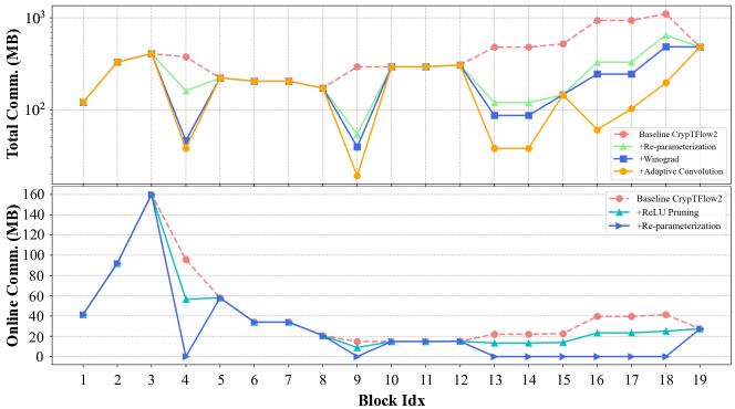
Figure 9: Block-wise visualization of online and total communication with different techniques on CoPriv-w0.75 on CIFAR-100.

5.6 Effectiveness of Communication-Aware Regularization

To show the effectiveness and importance of introducing communication-aware regularization $\mathcal{L}_{comm}$ formulated in Eq. 2, we compare our pruning method with $\mathcal{L}_{comm}$ and pruning methods of SNL cho2022selective and SENet kundu2023learning without $\mathcal{L}_{comm}$ in Figure 10. As we can observe, $\mathcal{L}_{comm}$ indeed helps to focus the pruning on the later layers, which incur more communication cost, and penalizes the costly blocks (e.g., block # 16 and # 18). In contrast, SNL does not take communication cost into consideration and SENet (ReLU sensitivity based) focuses on pruning early layers with more ReLUs, both of which incur huge communication overhead.

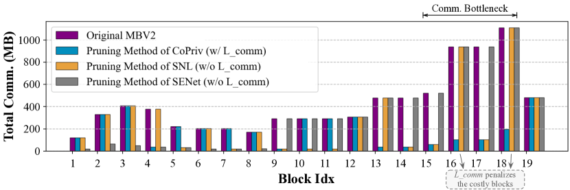
Figure 10: Comparison of different pruning method and the influence of $\mathcal{L}_{comm}$ during the search in each block (ReLU budget is set to 60% in this example).

6 Conclusion

In this work, we propose a network/protocol co-optimization framework, CoPriv, that simultaneously optimizes the pre-processing and online communication for the 2PC-based private inference. CoPriv features an optimized convolution protocol based on Winograd transformation and leverages a series of DNN-aware protocol optimization to improve the efficiency of the pre-processing stage. We also propose a differentiable communication-aware ReLU pruning algorithm with network re-parameterization to further optimize both the online and pre-processing communication induced by ReLU, truncation and convolution. With extensive experiments, CoPriv consistently reduces both online and total communication without compromising the accuracy compared with different prior-art efficient networks and network optimization algorithms.

Appendix A Related Works

Private inference has been a promising solution to protect both data and model privacy during deep learning inference. In recent years, there has been an increasing amount of literature on efficient private inference. According to the optimization technique, these works can be categorized into three types, i.e., 1) protocol optimization; 2) network optimization; and 3) joint optimization.

In protocol optimization, ABY demmler2015aby provides a highly efficient conversion between arithmetic sharing, boolean sharing and Yao’s sharing, and construct mixed protocols. As an extension, ABY3 mohassel2018aby3 switches back and forth between three secret sharing schemes using three-party computation (3PC). CypTFlow2 rathee2020cryptflow2 proposes a new protocol for secure and comparison and division which enables effecient non-linear operations such as ReLU. SiRNN rathee2021sirnn further proposes 2PC protocols for bitwidth extension, mixed-precision linear and non-linear operations. CrypTen knott2021crypten proposes a software framework that provides a flexible machine learning focused API. More recently, SecFloat rathee2022secfloat proposes the crypto-friendly precise functionalities to build a library for 32-bit single-precision floating-point operations and math functions. These works lack consideration for neural network architecture and has limited communication reduction.

In network optimization, DeepReDuce jha2021deepreduce proposes to manually remove ReLUs with a three-step optimization pipline. SNL cho2022selective proposes ReLU-aware optimization that leverages gradient-based NAS to selectively linearize a subset of ReLUs. CryptoNAS ghodsi2020cryptonas uses ReLU budget as a proxy and leverages NAS to tailor ReLUs. PolyMPCNet peng2022polympcnet and SAFENet lou2021safenet replace ReLUs with MPC-friendly polynomial, while Sphynx cho2022sphynx proposes an MPC-friendly ReLU-efficient micro-search space. SENet kundu2023learning innovatively measures the ReLU importance via layer pruning sensitivity and automatically optimize the network to meet the target ReLU budget. DeepReShape jha2021deepreduce finds that wider networks are more ReLU-efficient than the deeper ones and designs ReLU-efficient baseline networks with with FLOPs-ReLU-Accuracy balance. For Transformer-based models, MPCFormer li2022mpcformer proposes to simplify Softmax by replacing exponential with a more MPC-friendly quadratic operation. MPCViT zeng2023mpcvit proposes to mix both high accuracy and high efficiency attention variants to accelerate private Vision Transformer (ViT) inference. Network optimization mainly focuses on ReLU reduction which dominates the online communication, but total communication including convolution and truncation cannot be optimized.

Unluckily, only using either protocol or network optimization just leads to limited efficiency improvement. Delphi srinivasan2019delphi jointly optimizes cryptographic protocols and network by gradually replacing ReLU with quadratic approximation. COINN hussain2021coinn simultaneously optimizes quantized network and protocols with ciphertext-aware quantization and automated bitwidth configuration. Recently, ganesan2022efficient proposes to use Winograd convolution for reducing the number of multiplications and design the efficient convolution operation to reduce the communication cost. However, it does not take private inference into consideration for Winograd algorithm, and still suffers tremendous communication overhead. In this work, we jointly optimize the network and protocol and fully consider their coupling properties.

Appendix B Details of Experimental Setup

Private inference framework

CoPriv is built based on CypTFlow2 rathee2020cryptflow2 protocol for private inference. We leverage the Athos rathee2020cryptflow2 tool chain to convert both input and weight into fixed-point with the bit-width 41 and scale 12. We measure the communication and latency under a LAN setting rathee2020cryptflow2 with 377 MBps bandwidth and 0.3ms echo latency. All of our experiments are evaluated on the Intel Xeon Gold 5220R CPU @ 2.20GHz.

Implementation of Winograd-based convolution protocol

The convolution protocol with Winograd transformation and optimization is implemented in C++ with Eigen and Armadillo matrix calculation library sanderson2016armadillo in the CrypTFlow2 rathee2020cryptflow2 framework. We implement $F(2\times 2,3\times 3)$ and $F(4\times 4,3\times 3)$ transformation for convolution with stride of 1 and $F(2\times 2,3\times 3)$ transformation when stride is 2 huang2021efficient . For CIFAR-100 dataset, we use $F(2\times 2,3\times 3)$ transformation as the image resolution is small and for ImageNet dataset, we use $F(4\times 4,3\times 3)$. We only apply $F(2\times 2,3\times 3)$ for stride of 2 on ImageNet dataset. When evaluating CoPriv, we determine the optimal sender according to the analysis in Table 3 before inference. Winograd implementation enables us to measure the communication cost and latency of each convolution module.

Networks and datasets

We apply our proposed CoPriv to the widely used lightweight mobile network MobileNetV2 sandler2018mobilenetv2 with different width multipliers, e.g., 0.75, 1.0 and 1.4 to trade off the model accuracy and efficiency. We evaluate the top-1 accuracy and online and total communication on both CIFAR-100 and ImageNet deng2009imagenet dataset.

Differentiable pruning and finetuning setups

We first search and prune redundant ReLUs for 10 epochs and then finetune the pruned network for 180 epochs with stochastic gradient descent (SGD) optimizer amari1993backpropagation , cosine learning scheduler and initial learning rate of 0.1. During finetuning stage, we train our proposed CoPriv with knowledge distillation to boost its performance.

Appendix C Network Re-Parameterization Algorithm

Network (or structural) re-parameterization is a useful technique proposed by RepVGG ding2021repvgg , and is extended to ding2019acnet ; ding2022repmlpnet ; ding2021diverse ; fu2022depthshrinker ; ding2021resrep . The core idea of re-parameterization is to decouple the training-time architecture (with high performance and low efficiency) and inference-time network architecture (with equivalent performance and high efficiency). Re-parameterization is realized by converting one architecture to another via equivalently merging parameters together. Therefore, during inference time, the network architecture is not only efficient but also has the same high performance as the training-time architecture. Figure 11 is an simple example of re-parameterization.

Figure 11: An example of re-parameterization for batch normalization and convolution filter.

In this work, we can also leverage this technique to merge adjacent convolutions together after ReLU removal. For the network re-parameterization mentioned in Section 4.2, here we provide the following detailed algorithm 1 to equivalently merge the inverted residual block into a single dense convolution as shown in Figure 3. With the help of network re-parameterization, we further optimize the total communication including convolution and truncation.

1

2

Input : An inverted residual block with weights $W_{1\times 1}$, $W_{3\times 3}$, and $W^{\prime}_{1\times 1}$. The number of input and output channels $N_{in},N_{out}$. The size of re-parameterized weights $r$.

Output : Regular convolution with re-parameterized weights $W_{r}$.

3

4$W_{r}=$ torch.eye($N_{in}$);

5 $W_{r}=W_{r}$.unsqueeze(2).unsqueeze(2);

6 $W_{r}=$ torch.nn.functional.pad($W_{r}$, pad=($\frac{r-1}{2}$, $\frac{r-1}{2}$, $\frac{r-1}{2}$, $\frac{r-1}{2}$));

7 $W_{r}=$ torch.nn.functional.conv2d($W_{r},W_{1\times 1}$);

8 $W_{r}=$ torch.nn.functional.conv2d($W_{r},W_{3\times 3}$, padding=$\frac{r-1}{2}$);

9 $W_{r}=$ torch.nn.functional.conv2d($W_{r},W^{\prime}_{1\times 1}$);

10

11$W_{res}=$ torch.zeros($N_{out},N_{in},r,r$);

12 for $i\in[0,\ldots,N_{out}-1]$ do

13       $W_{res}[i,i,\lfloor r/2\rfloor,\lfloor r/2\rfloor]=1$;

14      

15$W_{r}=W_{r}+W_{res}$;

16

17return $W_{r}$;

18

Algorithm 1 Network Re-parameterization for Inverted Residual Block

Appendix D Details of Winograd Convolution

D.1 Comparison between Regular Convolution and Winograd Convolution

To help readers better understand the multiplication reduction of Winograd convolution, we demonstrate regular convolution and Winograd convolution in Figure 12. Given an input $I\in\mathbb{R}^{4\times 4}$ and a filter $F\in\mathbb{R}^{3\times 3}$, regular convolution requires $9\times 4=36$ times multiplications (implemented using GEMM with im2col algorithm chellapilla2006high ) while $F(2\times 2,3\times 3)$ Winograd transformation only requires $16\times 1=16$ times multiplications (EWMM), which achieves 2.25$\times$ reduction. Moreover, $F(4\times 4,3\times 3)$ with a larger tile size, i.e., 6 can further achieve 4$\times$ multiplication reduction. The improvement gets benefit from the Winograd’s ability to convert im2col to EWMM and calculate the whole tile in Winograd domain at once.

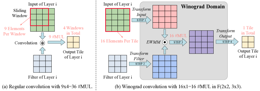
Figure 12: Comparison between (a) regular convolution and (b) Winograd convolution.

D.2 Details of Input Tiling and Padding

Given a large 2D input $I\in\mathbb{R}^{l\times l}$, where $l>m+r-1$, the core technique for ensuring the equivalence of regular convolution and Winograd convolution is input tiling and padding. The output size $l^{\prime}=l-r+1$, the input tile size $n=m+r-1$ and the total tile number $T$ per channel is computed as

$$T=\lceil\frac{l^{\prime}}{n}\rceil^{2}=\lceil\frac{l-r+1}{m+r-1}\rceil^{2},$$

where $\lceil\cdot\rceil$ denotes taking the upper bound value. For each tile, Winograd convolution is individually performed and results an output tile with $m\times m$ size. After all the tiles are computed with Winograd convolution, the output tiles are concatenated together to form the final output.

For some input size, the input cannot be covered by tiles. For instance, when leveraging $F(2\times 2,3\times 3)$ on the input $I\in\mathbb{R}^{7\times 7}$, the rightmost and bottom pixels cannot be divided into a complete tile. To solve this problem, we pad these positions with 0 to enable the tiles totally cover the whole input. The correctness and equivalence can be proved with Eq. 1. Also, ganesan2022efficient shows the overhead caused by padding is negligible.

D.3 Support for Stride of 2 Winograd Convolution

Conventional Winograd convolution only supports stride $s=1$ convolution filter. However, in recent efficient neural networks, e.g., MobileNetV2, EfficientNet has several stride of 2 layers to reduce the feature map size by half. To enable extreme optimization for efficient networks, we introduce $F(2\times 2,3\times 3)$ for stride of 2 Winograd convolution for private inference.

There are various methods to construct stride of 2 Winograd kernel such as dividing input and convolution filter into different groups yepez2020stride . However, it is not a simple way to implement stride of 2 Winograd kernel. huang2021efficient is an extremely convenient method using unified transformation matrices.

Based on huang2021efficient , even positions of input and filter are computed by $F(2,2)$ while odd positions are computed by regular convolution. Transformation matrices are derived as follows and can be computed using Eq. 1:

$$B^{\top}=\begin{bmatrix}1&0&-1&0&0\\ 0&1&0&0&0\\ 0&0&1&0&0\\ 0&0&0&1&0\\ 0&0&-1&0&1\end{bmatrix},\quad G=\begin{bmatrix}1&0&0\\ 0&1&0\\ 1&0&1\\ 0&1&0\\ 0&0&1\end{bmatrix},\quad A^{\top}=\begin{bmatrix}1&1&1&0&0\\ 0&0&1&1&1\\ \end{bmatrix}.$$

Correctness analysis.

Here, we take a 1D algorithm as an example to prove the correctness Winograd convolution for stride of 2. The algorithm can be nested with itself to obtain a 2D algorithm lavin2016fast .

Given input $X$ and filter $F$ as

$$X=\begin{bmatrix}x_{0}\\ x_{1}\\ x_{2}\\ x_{3}\\ x_{4}\end{bmatrix},\quad F=\begin{bmatrix}y_{0}\\ y_{1}\\ y_{2}\end{bmatrix},\quad Y=X\circledast F=\begin{bmatrix}z_{0}\\ z_{1}\end{bmatrix}.$$

First, we calculate regular convolution with stride of 2 using im2col algorithm chellapilla2006high as

$$Y_{1}=\begin{bmatrix}x_{0}&x_{1}&x_{2}\\ x_{2}&x_{3}&x_{4}\end{bmatrix}\cdot\begin{bmatrix}y_{0}\\ y_{1}\\ y_{2}\end{bmatrix}=\begin{bmatrix}x_{0}y_{0}+x_{1}y_{1}+x_{2}y_{2}\\ x_{2}y_{0}+x_{3}y_{1}+x_{4}y_{2}\end{bmatrix},$$

thus, $z_{0}=x_{0}y_{0}+x_{1}y_{1}+x_{2}y_{2}$ and $z_{1}=x_{2}y_{0}+x_{3}y_{1}+x_{4}y_{2}$.

Then, we calculate Winograd convolution for stride of 2 as

$$Y=A^{\top}\cdot[(GF)\odot(B^{\top}X)],$$

and then

$$Y_{2}=\begin{bmatrix}1&1&1&0&0\\ 0&0&1&1&1\end{bmatrix}\cdot[(\begin{bmatrix}1&0&0\\ 0&1&0\\ 1&0&1\\ 0&1&0\\ 0&0&1\end{bmatrix}\cdot\begin{bmatrix}y_{0}\\ y_{1}\\ y_{2}\end{bmatrix})\odot(\begin{bmatrix}1&0&-1&0&0\\ 0&1&0&0&0\\ 0&0&1&0&0\\ 0&0&0&1&0\\ 0&0&-1&0&1\end{bmatrix}\cdot\begin{bmatrix}x_{0}\\ x_{1}\\ x_{2}\\ x_{3}\\ x_{4}\end{bmatrix})],$$

and further simplify the calculation as

$$Y_{2}=\begin{bmatrix}1&1&1&0&0\\ 0&0&1&1&1\end{bmatrix}\cdot[(\begin{bmatrix}y_{0}\\ y_{1}\\ y_{0}+y_{2}\\ y_{1}\\ y_{2}\end{bmatrix})\odot(\begin{bmatrix}x_{0}-x_{2}\\ x_{1}\\ x_{2}\\ x_{3}\\ x_{4}-x_{2}\end{bmatrix})]=\begin{bmatrix}1&1&1&0&0\\ 0&0&1&1&1\end{bmatrix}\cdot\begin{bmatrix}x_{0}y_{0}-x_{2}y_{0}\\ x_{1}y_{1}\\ x_{2}y_{0}+x_{2}y_{2}\\ x_{3}y_{1}\\ x_{4}y_{2}-x_{2}y_{2}\end{bmatrix},$$

therefore, the convolution result is

$$Y_{2}=\begin{bmatrix}x_{0}y_{0}+x_{1}y_{1}+x_{2}y_{2}\\ x_{2}y_{0}+x_{3}y_{1}+x_{4}y_{2}\end{bmatrix}=Y_{1}.$$

D.4 Transformation Matrices for Winograd Convolution

We provide the transformation matrices $A,B,G$ for $F(2\times 2,3\times 3)$ and $F(4\times 4,3\times 3)$ Winograd transformation based on polynomial Chinese remainder theorem (CRT) or Lagrange interpolation lavin2016fast .

For $F(2\times 2,3\times 3)$, we have

$$B^{\top}=\begin{bmatrix}1&0&-1&0\\ 0&1&1&0\\ 0&-1&1&0\\ 0&1&0&-1\end{bmatrix},\quad G=\begin{bmatrix}1&0&0\\ 1/2&1/2&1/2\\ 1/2&-1/2&1/2\\ 0&0&1\\ \end{bmatrix},\quad A^{\top}=\begin{bmatrix}1&1&1&0\\ 0&1&-1&-1\end{bmatrix}.$$

For $F(4\times 4,3\times 3)$, we have

$$B^{\top}=\begin{bmatrix}4&0&-5&0&1&0\\ 0&-4&-4&1&1&0\\ 0&4&-4&-1&1&0\\ 0&-2&-1&2&1&0\\ 0&2&-1&-2&1&0\\ 0&4&0&-5&0&1\end{bmatrix},\quad G=\begin{bmatrix}1/4&0&0\\ -1/6&-1/6&-1/6\\ -1/6&1/6&-1/6\\ 1/24&1/12&1/6\\ 1/24&-1/12&1/6\\ 0&0&1\end{bmatrix},$$

$$A^{\top}=\begin{bmatrix}1&1&1&1&1&0\\ 0&1&-1&2&-2&0\\ 0&1&1&4&4&0\\ 0&1&-1&8&-8&1\end{bmatrix}.$$

The correctness analysis is the same with Section D.3.

Appendix E Comparison with More Related Work

kundu2023making is a recent work that aims at optimizing the network architecture for latency-efficient private inference. Both CoPriv and kundu2023making aim to reduce the number of ReLUs and the depth of the whole network in order to improve the efficiency. However, they have totally different motivations and methods. 1) Motivations: kundu2023making still regards ReLU as the main latency bottleneck and removes convolution layers to reduce computation. In contrast, CoPriv fuses neighboring convolution layers to better leverage our Winograd-based optimization for communication reduction of all operators. The difference in motivation leads to different criterion when selecting convolutions to remove. kundu2023making selects convolutions based on ReLU sensitivity kundu2023learning while CoPriv simultaneously considers both accuracy and communication cost. 2) Methods: kundu2023making first determines which convolutions to remove based on ReLU sensitivity kundu2023learning and then, uses the gated branching method for training. In contrast, CoPriv simultaneously train the architecture parameters with the model weights, and the equivalent re-parameterization is conducted post training, enabling us to leverage the benefits of over-parameterization during training shown in RepVGG ding2021repvgg . Quantitatively, we compare CoPriv with kundu2023making in Table 5. CoPriv achieves much lower online and total communication while achieving higher accuracy compared to kundu2023making .

Table 5: Accuracy and communication comparison between CoPriv and kundu2023making .

Method	Top-1 Acc. (%)	Online Comm. (GB)	Total Comm. (GB)
kundu2023making	69.10	0.81	46.5
CoPriv (ours)	70.58	0.43	5.14

Appendix F More Detailed Comparison with Prior-Art Methods

As a supplement of Table 2, we provide a more detailed comparison with prior-art methods in terms of different techniques in Table 6.

Table 6: Comparison with prior-art methods in terms of different techniques.

Method	Protocol Optimization	Network Optimization
		Convolution	Truncation	ReLU
rathee2020cryptflow2 ; rathee2021sirnn ; mohassel2017secureml ; demmler2015aby ; mohassel2018aby3 ; knott2021crypten ; rathee2022secfloat	ReLU, Trunc, Conv.	✗	✗	✗
kundu2023learning ; cho2022selective ; ghodsi2020cryptonas ; peng2022polympcnet ; lou2021safenet ; cho2022sphynx ; jha2023deepreshape ; jha2021deepreduce	✗	✗	✗	ReLU count/sensitivity-aware NAS
srinivasan2019delphi ; hussain2021coinn	Conv. (Online to Offline)	✗	✗	ReLU count-aware NAS
ganesan2022efficient	Conv. (Winograd-based)	Factorized Point-wise Conv.	✗	✗
liu2019metapruning	✗	Channel Reduction	Channel Reduction	Channel Reduction
CoPriv (ours)	Conv. (Winograd-based)	Re-paramerization	Re-paramerization	Communication-aware NAS

Appendix G Comparison of Convolution Protocol with HE-Based Method

We also compare CoPriv with SOTA homomorphic encryption (HE) based method, Cheetah huang2022cheetah , which uses HE-based protocol for convolution instead of oblivious transfer (OT) in CrypTFlow2. Cheetah achieves lower communication compared to CrypTFlow2 at the cost of more computation overhead for both the server and client. Here, we compare their inference latency. Hence, we believe Cheetah and CrypTFlow2/CoPriv have different applicable scenarios. For example, for less performant clients, Cheetah may not be applicable, while when the bandwidth is low, CrypTFlow2/CoPriv may not be the best choice. When comparing CoPriv with Cheetah, we observe a similar trend. As shown in Table 7, we find while CoPriv always outperforms CrypTFlow2, for high bandwidth, CoPriv achieves lower latency compared to Cheetah while for low bandwidth, Cheetah incurs lower latency.

Table 7: Convolution latency (s) comparison with Cheetah for different blocks (expand ratio is set to 6) and bandwidths.

Bandwidth	384 MBps huang2022cheetah	44 MBps huang2022cheetah	9 MBps shen2022abnn2 ; mohassel2017secureml
Dimension: $(4\times 4\times 64)$
Baseline OT (CrypTFlow2)	2.14	3.55	16.2
HE (Cheetah)	1.35	1.54	2.99
CoPriv w/ Winograd (ours)	0.21	0.64	3.00
Dimension: $(8\times 8\times 32)$
Baseline OT (CrypTFlow2)	1.29	3.94	16.1
HE (Cheetah)	0.72	0.73	1.53
CoPriv w/ Winograd (ours)	0.17	0.45	2.16

References

- [1] Syed Asad Alam, Andrew Anderson, Barbara Barabasz, and David Gregg. Winograd convolution for deep neural networks: Efficient point selection. ACM Transactions on Embedded Computing Systems, 21(6):1–28, 2022.
- [2] Shun-ichi Amari. Backpropagation and stochastic gradient descent method. Neurocomputing, 5(4-5):185–196, 1993.
- [3] Barbara Barabasz, Andrew Anderson, Kirk M Soodhalter, and David Gregg. Error analysis and improving the accuracy of winograd convolution for deep neural networks. ACM Transactions on Mathematical Software (TOMS), 46(4):1–33, 2020.
- [4] Yoshua Bengio, Nicholas Léonard, and Aaron Courville. Estimating or propagating gradients through stochastic neurons for conditional computation. arXiv preprint arXiv:1308.3432, 2013.
- [5] Kumar Chellapilla, Sidd Puri, and Patrice Simard. High performance convolutional neural networks for document processing. In Tenth international workshop on frontiers in handwriting recognition. Suvisoft, 2006.
- [6] Minsu Cho, Zahra Ghodsi, Brandon Reagen, Siddharth Garg, and Chinmay Hegde. Sphynx: A deep neural network design for private inference. IEEE Security & Privacy, 20(5):22–34, 2022.
- [7] Minsu Cho, Ameya Joshi, Brandon Reagen, Siddharth Garg, and Chinmay Hegde. Selective network linearization for efficient private inference. In International Conference on Machine Learning, pages 3947–3961. PMLR, 2022.
- [8] Daniel Demmler, Thomas Schneider, and Michael Zohner. Aby-a framework for efficient mixed-protocol secure two-party computation. In NDSS, 2015.
- [9] Jia Deng, Wei Dong, Richard Socher, Li-Jia Li, Kai Li, and Li Fei-Fei. Imagenet: A large-scale hierarchical image database. In 2009 IEEE conference on computer vision and pattern recognition, pages 248–255. Ieee, 2009.
- [10] Xiaohan Ding, Honghao Chen, Xiangyu Zhang, Jungong Han, and Guiguang Ding. Repmlpnet: Hierarchical vision mlp with re-parameterized locality. In Proceedings of the IEEE/CVF Conference on Computer Vision and Pattern Recognition, pages 578–587, 2022.
- [11] Xiaohan Ding, Yuchen Guo, Guiguang Ding, and Jungong Han. Acnet: Strengthening the kernel skeletons for powerful cnn via asymmetric convolution blocks. In Proceedings of the IEEE/CVF international conference on computer vision, pages 1911–1920, 2019.
- [12] Xiaohan Ding, Tianxiang Hao, Jianchao Tan, Ji Liu, Jungong Han, Yuchen Guo, and Guiguang Ding. Resrep: Lossless cnn pruning via decoupling remembering and forgetting. In Proceedings of the IEEE/CVF International Conference on Computer Vision, pages 4510–4520, 2021.
- [13] Xiaohan Ding, Xiangyu Zhang, Jungong Han, and Guiguang Ding. Diverse branch block: Building a convolution as an inception-like unit. In Proceedings of the IEEE/CVF Conference on Computer Vision and Pattern Recognition, pages 10886–10895, 2021.
- [14] Xiaohan Ding, Xiangyu Zhang, Ningning Ma, Jungong Han, Guiguang Ding, and Jian Sun. Repvgg: Making vgg-style convnets great again. In Proceedings of the IEEE/CVF conference on computer vision and pattern recognition, pages 13733–13742, 2021.
- [15] Javier Fernandez-Marques, Paul Whatmough, Andrew Mundy, and Matthew Mattina. Searching for winograd-aware quantized networks. Proceedings of Machine Learning and Systems, 2:14–29, 2020.
- [16] Yonggan Fu, Haichuan Yang, Jiayi Yuan, Meng Li, Cheng Wan, Raghuraman Krishnamoorthi, Vikas Chandra, and Yingyan Lin. Depthshrinker: a new compression paradigm towards boosting real-hardware efficiency of compact neural networks. In International Conference on Machine Learning, pages 6849–6862. PMLR, 2022.
- [17] Vinod Ganesan, Anwesh Bhattacharya, Pratyush Kumar, Divya Gupta, Rahul Sharma, and Nishanth Chandran. Efficient ml models for practical secure inference. arXiv preprint arXiv:2209.00411, 2022.
- [18] Karthik Garimella, Zahra Ghodsi, Nandan Kumar Jha, Siddharth Garg, and Brandon Reagen. Characterizing and optimizing end-to-end systems for private inference. In ACM International Conference on Architectural Support for Programming Languages and Operating Systems (ASPLOS), ASPLOS 2023, page 89–104, New York, NY, USA, 2023. Association for Computing Machinery.
- [19] Zahra Ghodsi, Akshaj Kumar Veldanda, Brandon Reagen, and Siddharth Garg. Cryptonas: Private inference on a relu budget. Advances in Neural Information Processing Systems, 33:16961–16971, 2020.
- [20] Kaiming He, Xiangyu Zhang, Shaoqing Ren, and Jian Sun. Deep residual learning for image recognition. In Proceedings of the IEEE conference on computer vision and pattern recognition, pages 770–778, 2016.
- [21] Geoffrey Hinton, Oriol Vinyals, and Jeff Dean. Distilling the knowledge in a neural network. arXiv preprint arXiv:1503.02531, 2015.
- [22] Andrew Howard, Mark Sandler, Grace Chu, Liang-Chieh Chen, Bo Chen, Mingxing Tan, Weijun Wang, Yukun Zhu, Ruoming Pang, Vijay Vasudevan, et al. Searching for mobilenetv3. In Proceedings of the IEEE/CVF international conference on computer vision, pages 1314–1324, 2019.
- [23] Chengcheng Huang, Xiaoxiao Dong, Zhao Li, Tengteng Song, Zhenguo Liu, and Lele Dong. Efficient stride 2 winograd convolution method using unified transformation matrices on fpga. In 2021 International Conference on Field-Programmable Technology (ICFPT), pages 1–9. IEEE, 2021.
- [24] Zhicong Huang, Wen-jie Lu, Cheng Hong, and Jiansheng Ding. Cheetah: Lean and fast secure Two-Party deep neural network inference. In 31st USENIX Security Symposium (USENIX Security 22), pages 809–826, 2022.
- [25] Siam Umar Hussain, Mojan Javaheripi, Mohammad Samragh, and Farinaz Koushanfar. Coinn: Crypto/ml codesign for oblivious inference via neural networks. In Proceedings of the 2021 ACM SIGSAC Conference on Computer and Communications Security, pages 3266–3281, 2021.
- [26] Nandan Kumar Jha, Zahra Ghodsi, Siddharth Garg, and Brandon Reagen. Deepreduce: Relu reduction for fast private inference. In International Conference on Machine Learning, pages 4839–4849. PMLR, 2021.
- [27] Nandan Kumar Jha and Brandon Reagen. Deepreshape: Redesigning neural networks for efficient private inference. arXiv preprint arXiv:2304.10593, 2023.
- [28] Chiraag Juvekar, Vinod Vaikuntanathan, and Anantha Chandrakasan. GAZELLE: A low latency framework for secure neural network inference. In 27th USENIX Security Symposium (USENIX Security 18), pages 1651–1669, 2018.
- [29] Brian Knott, Shobha Venkataraman, Awni Hannun, Shubho Sengupta, Mark Ibrahim, and Laurens van der Maaten. Crypten: Secure multi-party computation meets machine learning. Advances in Neural Information Processing Systems, 34:4961–4973, 2021.
- [30] Alex Krizhevsky, Geoffrey Hinton, et al. Learning multiple layers of features from tiny images. 2009.
- [31] Nishant Kumar, Mayank Rathee, Nishanth Chandran, Divya Gupta, Aseem Rastogi, and Rahul Sharma. Cryptflow: Secure tensorflow inference. In IEEE Symposium on Security and Privacy (SP), pages 336–353. IEEE, 2020.
- [32] Souvik Kundu, Shunlin Lu, Yuke Zhang, Jacqueline Liu, and Peter A Beerel. Learning to linearize deep neural networks for secure and efficient private inference. arXiv preprint arXiv:2301.09254, 2023.
- [33] Souvik Kundu, Yuke Zhang, Dake Chen, and Peter A Beerel. Making models shallow again: Jointly learning to reduce non-linearity and depth for latency-efficient private inference. In Proceedings of the IEEE/CVF Conference on Computer Vision and Pattern Recognition, pages 4684–4688, 2023.
- [34] Andrew Lavin and Scott Gray. Fast algorithms for convolutional neural networks. In Proceedings of the IEEE conference on computer vision and pattern recognition, pages 4013–4021, 2016.
- [35] Dacheng Li, Rulin Shao, Hongyi Wang, Han Guo, Eric P Xing, and Hao Zhang. Mpcformer: fast, performant and private transformer inference with mpc. arXiv preprint arXiv:2211.01452, 2022.
- [36] Zechun Liu, Haoyuan Mu, Xiangyu Zhang, Zichao Guo, Xin Yang, Kwang-Ting Cheng, and Jian Sun. Metapruning: Meta learning for automatic neural network channel pruning. In Proceedings of the IEEE/CVF international conference on computer vision, pages 3296–3305, 2019.
- [37] Qian Lou, Yilin Shen, Hongxia Jin, and Lei Jiang. Safenet: A secure, accurate and fast neural network inference. In International Conference on Learning Representations, 2021.
- [38] Payman Mohassel and Peter Rindal. Aby3: A mixed protocol framework for machine learning. In ACM SIGSAC conference on computer and communications security, pages 35–52, 2018.
- [39] Payman Mohassel and Yupeng Zhang. Secureml: A system for scalable privacy-preserving machine learning. In 2017 IEEE symposium on security and privacy (SP), pages 19–38. IEEE, 2017.
- [40] Hongwu Peng, Shanglin Zhou, Yukui Luo, Shijin Duan, Nuo Xu, Ran Ran, Shaoyi Huang, Chenghong Wang, Tong Geng, Ang Li, et al. Polympcnet: Towards relu-free neural architecture search in two-party computation based private inference. arXiv preprint arXiv:2209.09424, 2022.
- [41] Deevashwer Rathee, Anwesh Bhattacharya, Rahul Sharma, Divya Gupta, Nishanth Chandran, and Aseem Rastogi. Secfloat: Accurate floating-point meets secure 2-party computation. In 2022 IEEE Symposium on Security and Privacy (SP), pages 576–595. IEEE, 2022.
- [42] Deevashwer Rathee, Mayank Rathee, Rahul Kranti Kiran Goli, Divya Gupta, Rahul Sharma, Nishanth Chandran, and Aseem Rastogi. Sirnn: A math library for secure rnn inference. In 2021 IEEE Symposium on Security and Privacy (SP), pages 1003–1020. IEEE, 2021.
- [43] Deevashwer Rathee, Mayank Rathee, Nishant Kumar, Nishanth Chandran, Divya Gupta, Aseem Rastogi, and Rahul Sharma. Cryptflow2: Practical 2-party secure inference. In Proceedings of the 2020 ACM SIGSAC Conference on Computer and Communications Security, pages 325–342, 2020.
- [44] Brandon Reagen, Woo-Seok Choi, Yeongil Ko, Vincent T Lee, Hsien-Hsin S Lee, Gu-Yeon Wei, and David Brooks. Cheetah: Optimizing and accelerating homomorphic encryption for private inference. In IEEE International Symposium on High-Performance Computer Architecture (HPCA), pages 26–39. IEEE, 2021.
- [45] Conrad Sanderson and Ryan Curtin. Armadillo: a template-based c++ library for linear algebra. Journal of Open Source Software, 1(2):26, 2016.
- [46] Mark Sandler, Andrew Howard, Menglong Zhu, Andrey Zhmoginov, and Liang-Chieh Chen. Mobilenetv2: Inverted residuals and linear bottlenecks. In Proceedings of the IEEE conference on computer vision and pattern recognition, pages 4510–4520, 2018.
- [47] Liyan Shen, Ye Dong, Binxing Fang, Jinqiao Shi, Xuebin Wang, Shengli Pan, and Ruisheng Shi. Abnn2: secure two-party arbitrary-bitwidth quantized neural network predictions. In Proceedings of the 59th ACM/IEEE Design Automation Conference, pages 361–366, 2022.
- [48] Wenting Zheng Srinivasan, PMRL Akshayaram, and Popa Raluca Ada. Delphi: A cryptographic inference service for neural networks. In Proc. 29th USENIX Secur. Symp, pages 2505–2522, 2019.
- [49] Kevin Vincent, Kevin Stephano, Michael Frumkin, Boris Ginsburg, and Julien Demouth. On improving the numerical stability of winograd convolutions. 2017.
- [50] Juan Yepez and Seok-Bum Ko. Stride 2 1-d, 2-d, and 3-d winograd for convolutional neural networks. IEEE Transactions on Very Large Scale Integration (VLSI) Systems, 28(4):853–863, 2020.
- [51] Wenxuan Zeng, Meng Li, Wenjie Xiong, Tong Tong, Wen-jie Lu, Jin Tan, Runsheng Wang, and Ru Huang. Mpcvit: Searching for accurate and efficient mpc-friendly vision transformer with heterogeneous attention. In Proceedings of the IEEE/CVF International Conference on Computer Vision, pages 5052–5063, 2023.