Flexible Error Mitigation of Quantum Processes with Data Augmentation Empowered Neural Model

Abstract

Neural networks have shown their effectiveness in various tasks in the realm of quantum computing. However, their application in quantum error mitigation, a crucial step towards realizing practical quantum advancements, has been restricted by reliance on noise-free statistics. To tackle this critical challenge, we propose a data augmentation empowered neural model for error mitigation (DAEM). Our model does not require any prior knowledge about the specific noise type and measurement settings and can estimate noise-free statistics solely from the noisy measurement results of the target quantum process, rendering it highly suitable for practical implementation. In numerical experiments, we show the model’s superior performance in mitigating various types of noise, including Markovian noise and Non-Markovian noise, compared with previous error mitigation methods. We further demonstrate its versatility by employing the model to mitigate errors in diverse types of quantum processes, including those involving large-scale quantum systems and continuous-variable quantum states. This powerful data augmentation-empowered neural model for error mitigation establishes a solid foundation for realizing more reliable and robust quantum technologies in practical applications.

I Introduction

The development of quantum technologies has positioned them as game-changers, capable of unlocking new opportunities and advantages in computing, simulation, communication, and sensing. Nonetheless, the implementation of quantum information processing remains challenging. One of the most critical obstacles is the effect of noise, prevalent in quantum systems of all kinds, that distorts the output of quantum information processing and compromises the quantum superiority. As a result, major efforts have been directed towards the development of appropriate techniques for quantum error mitigation Cai et al. (2022), including zero-noise extrapolation (ZNE) Temme et al. (2017); Li and Benjamin (2017); Kandala et al. (2019); Kim et al. (2023a, b), Clifford data regression (CDR) Czarnik et al. (2021, 2022); Strikis et al. (2021); Lowe et al. (2021), probablistic error cancellation Temme et al. (2017); Endo et al. (2018); Van Den Berg et al. (2023), and virtual purification Huggins et al. (2021); Koczor (2021); Seif et al. (2023).

Deep neural networks have been utilized as a compelling tool in addressing many crucial tasks within the realm of quantum computing and quantum information including characterization of quantum systems Torlai et al. (2018); Zhu et al. (2022), quantum verification Wu et al. (2023), and quantum simulations Bennewitz et al. (2022). However, their application in quantum error mitigation has been constrained and their full potential in this domain still remains untapped, despite some previous attempts Kim et al. (2020); Liao et al. (2023); Zhukov and Pogosov (2022); Sack and Egger (2023). This mainly stems from the reliance on noise-free or low-noise measurement data, which is indispensable for previous machine learning algorithms to generate satisfactory mitigation results. On the other hand, as quantum processes in practice are noise-prone and complex to simulate, acquiring such data is often challenging. The insufficiency of such labeled data for training poses a significant obstacle to effectively exploiting deep neural networks for quantum error mitigation.

In order to tackle this challenge, we have innovatively integrated data augmentation techniques Shorten and Khoshgoftaar (2019); Taylor and Nitschke (2018) into the design of the model for quantum error mitigation. Data augmentation has proven particularly valuable in scenarios where the amount of available training data is limited. For example, in few-shot learning Wang et al. (2020), neural models are trained to recognize new objects or classes based on a very small set of examples. Zero-shot learning Wang et al. (2019) extends this idea to recognize objects or classes that are not given in training, relying on semantic attributes or textual descriptions. Motivated by its success in various tasks within classical machine learning, we introduce a data augmentation-empowered error mitigation model (DAEM), depicted in Figure 1, for various quantum processes, extending beyond the scope of quantum circuits. This model effectively leverages measurement statistics across a spectrum of unknown noise levels to make precise estimations of noise-free statistics of the target quantum process.

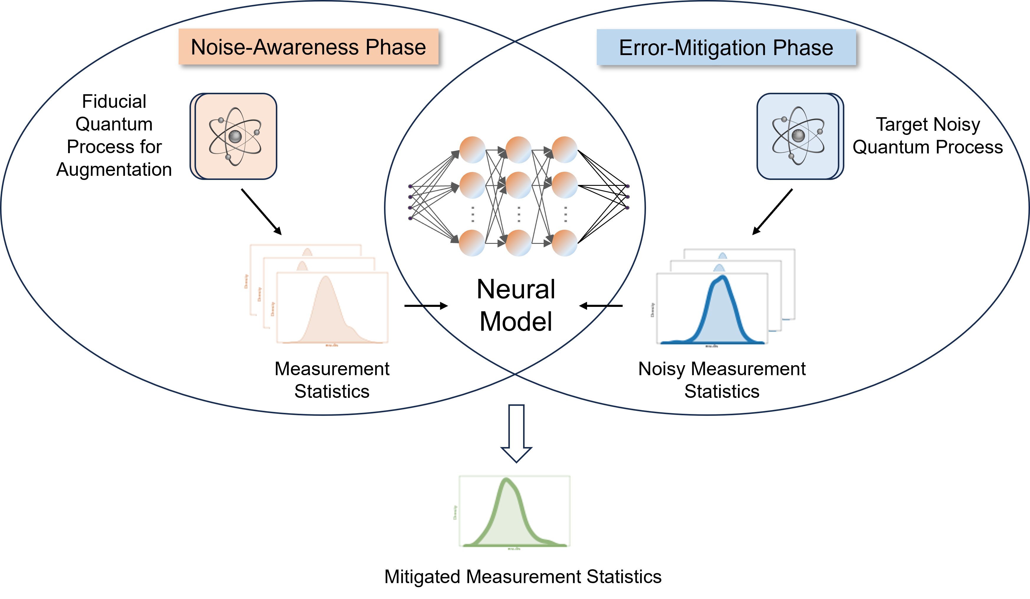
Figure 1: Framework of DAEM model. The entire procedure is divided into two phases. In the first phase, known as Noise-Awareness phase, we train the neural model for error mitigation with the assistance of a fiducial process. In the second phase, known as Error-Mitigation phase, we apply the trained neural model to mitigate the noisy measurement statistics collected from the target noisy quantum process.

Our proposed model exhibits three major characteristics compared to previous approaches. (1) Exemption from noise-free statistics reliance: Our proposed architecture eliminates the need for noise-free statistics acquired from the target quantum process. This feature allows the model to be potentially applicable in real-world experiments. Additionally, while our model still relies on noisy measurement data across different noise levels, it does not assume the knowledge of noise level values, an assumption commonly made by previous approaches that would require an extra noise estimation procedure in practice. (2) Versatility on various types of quantum processes: The proposed architecture is flexible and can accept different forms of measurement statistics as inputs, making it suitable for various quantum processes, including quantum circuits, continuous-variable quantum processes, and dynamics of large-scale spin systems. (3) Adaptability to diverse settings and noise models: Our data-driven model can be trained using measurement statistics without relying on rigid assumptions about noise models or requiring a specific initial state or measurement setting. Furthermore, it is capable of mitigating not only the error of observable expectations, but also the distortion of measurement probability distributions.

II Results

II.1 Framework

In this work, we propose a general setup , depicted in Figure 1, for quantum error mitigation. We denote the (noisy) quantum process for error mitigation by $\mathcal{N}_{\lambda}(\mathcal{E})$, wherein $\mathcal{E}$ is the ideal noiseless process, $\mathcal{N}_{\lambda}$ represents the noise model, and ${\lambda}$ is a parameter indicating the noise level. Instead of the full statistics of the output state, we focus on that generated by a set of measurements $\mathcal{M}$ of interest. In quantum algorithms and applications, $\mathcal{M}$ can represent a collection of quantum measurements conducted on various qubits to extract different pieces of information or characteristics of the quantum system. Within this set, each measurement $\bm{M}_{i}=\{M_{ij}\}_{j}$ in $\mathcal{M}$ is formulated as a positive operator-valued measure (POVM) composed of $m$ positive operators that satisfy the normalization condition $\sum_{j=1}^{m}M_{ij}=\mathds{1}$. We remark that this general setup covers tomography (when $\mathcal{M}$ is tomographically complete) and measuring single observables. On the other hand, the input state $\rho_{s}$ of the process can be randomly selected from a set $\mathcal{S}$, guided by a prescribed prior probability distribution, thereby encompassing a broader spectrum of initial states rather than being limited to a specific state. Here our goal is to estimate noise-free statistics for the output state, denoted as $\bm{p}_{is}^{(0)}=\{\operatorname{tr}(\mathcal{E}(\rho_{s})M_{ij})\}$, corresponding to any input state $\rho_{s}\in\mathcal{S}$ from $\mathcal{E}$ and any measurement $\bm{M}_{i}\in\mathcal{M}$.

In our setup, we assume the experimenter has access to both the target mitigation process, $\mathcal{N}_{\lambda}(\mathcal{E})$, and a fiducial process responsible for data augmentation, $\mathcal{N}_{\lambda}(\mathcal{F})$, which shares the same noise model with the target process and the same circuit template. The key feature of the fiducial process is that it allows us to easily derive the ideal output measurement statistics from the statistics of measurements conducted directly on the input states. A detailed explanation of the construction of $\mathcal{N}_{\lambda}(\mathcal{F})$ in different settings is provided in the Methods.

Initially, the experimenter gathers measurement statistics from the fiducial process $\mathcal{N}_{\lambda}(\mathcal{F})$ with $n$ randomly selected input states $\{\rho_{s_{1}}\}_{s_{1}=1}^{n}$, where $\forall\rho_{s_{1}}\in\mathcal{S}$, across a range of noise levels $\{\lambda_{k}\}_{k=1}^{K}$, where $\lambda_{k}>\lambda_{min}\leavevmode\nobreak\ \forall k\in[K]$ and $\lambda_{min}$ represents the minimum achievable noise level in the experiment. Note that we do not assume knowledge of the exact values of $\{\lambda_{k}\}_{k=1}^{K}$ and, consequently, do not require any extra noise estimation procedure in practice. These acquired measurement statistics are denoted as $\{{\bm{p}^{\prime}}_{is_{1}}^{(k)}\}$. Following this, the experimenter proceeds to collect measurement statistics for any designated target input state $\rho_{s}\in\mathcal{S}$ from the noisy process $\mathcal{N}_{\lambda}(\mathcal{E})$. This step also involves varying the noise levels $\{\lambda_{k}\}_{k=1}^{K}$ and the resulting acquired measurement statistics are denoted as $\{\bm{p}_{is}^{(k)}\}$.

We exploit a deep neural network-based model as the cornerstone of our DAEM model. The application of the DAEM model for error mitigation is divided into two phases. The initial phase, known as Noise-Awareness phase, involves training the neural model with the assistance of the fiducial process. During this phase, the neural model undergoes training, enabling it to autonomously discern and comprehend the intricacies of the noise within the target process in its own manner, thus preparing it for subsequent error mitigation. In this phase, we first formulate a training set for the neural model that comprises both the noisy and noise-free statistics of the fiducial process $\mathcal{N}_{\lambda}(\mathcal{F})$. This set is denoted as $\mathcal{T}=\{\bm{P}_{s_{1}},{\bm{p}^{\prime}}_{s_{1}}^{(0)}\}_{s_{1}=1}^{m}$, where $\bm{P}_{s_{1}}=({\bm{p}^{\prime}}_{s_{1}}^{(1)},\dots,{\bm{p}^{\prime}}_{s_{1}}^{(K)})$ and ${\bm{p}^{\prime}}_{s_{1}}^{(0)}$ represents the corresponding noise-free statistics, associated with $\rho_{s}$ and $\mathcal{M}$. It’s important to note that obtaining ${\bm{p}^{\prime}}_{s_{1}}^{(0)}$ can be achieved either through direct calculations or by deriving it from measurement statistics of the input states $\{\rho_{s_{1}}\}_{s_{1}=1}^{n}$. Subsequently, we optimize the parameters of the neural model using the training set $\mathcal{T}$, guided by a loss function $\mathcal{L}$ (See Methods for details). Once the Noise-Awareness phase is complete, the neural model becomes proficient at translating the noisy measurement statistics associated with a spectrum of unknown noise levels into their corresponding noise-free statistics.

In the second phase, named as the Error-Mitigation phase, we input the noisy statistics $\{\bm{p}_{is}^{(k)}\}$ – associated with the output states of $\rho_{s}$ from $\{\mathcal{N}_{\lambda_{k}}(\mathcal{E})\}_{k=1}^{K}$ – into the trained neural model. The neural model then outputs the inferred the ideal statistics ${\bm{p}_{is}^{(0)}}$ pertaining to $\mathcal{E}$. We stress that our trained neural model can be employed for the error mitigation of noisy measurement statistics associated with any input state $\rho\in\mathcal{S}$ during the Error-Mitigation phase, without a retraining of the neural network. Furthermore, it’s worth noting that we do not require any noise-free measurement data related to the ideal process, $\mathcal{E}$ throughout the entire procedure. Hence, the model can be readily extended to large-scale systems and real-world experiments where the classical simulation of quantum processes cannot be achieved. A detailed description of the implementation of the neural model in various settings is available in the Methods section and the Appendix.

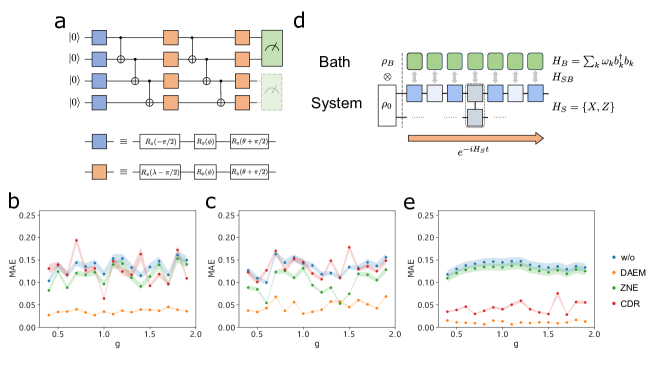
Figure 2: Variational quantum eigensolvers. a. The variational ansatz for preparing the ground states of 4-qubit transverse Ising models. b. Mean Absolute Errors (MAE) between the mitigated measurement expectation values for phase damping noise model and ideal expectation values. c. Mean Absolute Errors (MAE) between the mitigated measurement expectation values for amplitude damping noise model and ideal expectation values. d. Schematic diagram of quantum circuits affected by Non-Markovian noise. e. Mean Absolute Errors (MAE) between the mitigated measurement expectation values for considered Non-Markovian noise model and ideal expectation values.

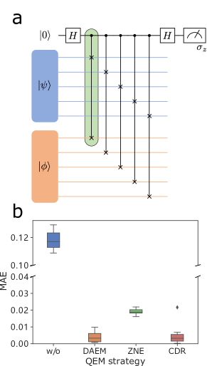
Figure 3: Swap Test. a. The swap test circuit for comparing two 5-qubit states. The gate within the green box is the controlled-SWAP gate. b. Mean Absolute Errors (MAE) between the mitigated fidelity values and the ground truth values.

II.2 Error Mitigation for Quantum Algorithms

The domain most suitable for testing our error mitigation model is quantum circuits, which are widely employed in various quantum algorithms.Our framework applies generally to quantum algorithms, where the goal is to obtain noise-free statistics from noisy quantum circuits. In this section, we test the performance of DAEM on prototypical NISQ algorithms, including the Variational Quantum Eigensolvers (VQEs) Peruzzo et al. (2014), the swap test Buhrman et al. (2001), and the Quantum Approximate Optimization Algorithm (QAOA) Farhi et al. (2014).

Variational quantum eigensolvers.

Variational Quantum Eigensolvers (VQEs), widely utilized in the realms of quantum chemistry and quantum computation, leverage parameterized quantum circuits to approximate the ground states of specified Hamiltonians. However, in practical scenarios, these circuits inevitably grapple with noise, leading to deviations in the ground state energy from the ideal scenario. In this context, we consider a scenario where an experimenter possesses the optimal parameters of a well-trained VQE circuit and intends to employ it on a real noisy quantum device. The experimenter’s goal is to derive the ideal measurement statistics of the ground state based on the gathered noisy measurement data.

In the following, we consider the VQEs for the transverse Ising chain with Hamiltonian

$$H_{\text{Ising}}=-g\sum_{i=1}^{N}X_{i}-J\sum_{i=1}^{N-1}Z_{i}Z_{i+1},$$ (1)

where $X$, $Z$ are Pauli operators, and $N$ is the number of qubits. The variational ansatz used to prepare the ground state is a hardware-efficient ansatz, composed of single-qubit Euler rotation gates and CNOT gates, as illustrated in Figure 2a. We choose $16$ circuits, varying the parameter $g$ within the range of $[0.4,2.0)$ with a stride of $0.1$. Additionally, we set the values of $J$ and $N$ to be $1$ and $4$ respectively for all experiments. For the set of measurements $\mathcal{M}$, we choose all two-qubit Pauli measurements on nearest-neighbor qubits. We let $\mathcal{S}$ be all of the $4$-qubit pure states and we randomly select $n=100$ states $\{\rho_{s_{1}}\}_{s_{1}=1}^{n}$ in the Noise-Awareness phase of all our experiments for each $g$. During the Error-Mitigation phase, we evaluate our mitigation model by using the prepared initial state $\rho_{0}=\ket{0}\bra{0}^{\otimes N}$.

First, we evaluate our model’s performance under two Markovian noise models: amplitude damping and phase damping. In all of the experiments, noise is applied after each gate in Figure 2a. The amplitude damping noise channel and the phase damping noise channel are mathematically defined by Equation 3 and Equation 6, respectively. Throughout all of our experiments, we consider a set of noise levels denoted as $\{\lambda_{k}\}_{k=1}^{K}\in[0.05,0.29]$, with stride 0.02.

$$\rho\rightarrow V_{0}\rho V_{0}^{\dagger}+V_{1}\rho V_{1}^{\dagger},$$ (2)

with $V_{0}=\begin{bmatrix}1&0\\ 0&\sqrt{1-\lambda}\end{bmatrix}$ and $V_{1}=\begin{bmatrix}0&\sqrt{\lambda}\\ 0&0\end{bmatrix}$. Figure 2b illustrates the mitigation results obtained using various error mitigation techniques for VQE circuits affected by phase damping noise, while Figure 2c presents the mitigation results for VQE circuits affected by amplitude damping noise. The results clearly demonstrate that DAEM consistently outperforms other mitigation methods for each VQE circuit, regardless of the specific value of $g$.

In addition to the Markovian noise model, we also investigate the impact of Non-Markovian noise, which, despite its relevance in real-world quantum experiments White et al. (2020); Agarwal et al. (2023); Groszkowski et al. (2023), has received limited attention in previous error mitigation studies. Specifically, we consider the multi-qubit spin-boson model Breuer and Petruccione (2007) for phase damping to exemplify this scenario, in which a quantum system interacts with environment, namely, a heat bath, and evolves jointly. This is a potential noise happening in superconducting quantum circuits Magazzù et al. (2018). In this setup, depicted in Figure 2d, the system Hamiltonian $H_{S}$ corresponds to the VQE circuit, while the heat bath is modeled as a bosonic system. We assume each gate in the circuit interacts independently with a bath attached locally. The bath Hamiltonian is $H_{B}=\sum_{k}\omega_{k}b_{k}^{\dagger}b_{k}$. Here $b_{k}$ is the annihilation operator for mode $k$, and $\omega_{k}$ is the corresponding energy. The interaction between the system and the bath is captured by the Hamiltonian $H_{SB}=\sum_{k}\sigma_{z}\otimes[\lambda_{k}b_{k}+\lambda_{k}^{*}b_{k}^{{\dagger}}]$, where $\sigma_{z}$ is Pauli-Z operator, and $\lambda_{k}\propto 1/\sqrt{\omega_{k}}$. We initiate the system and bath as a product state state $\rho_{0}\otimes\rho_{B}$, where $\rho_{0}$ is the initial state of the system, namely $|0\rangle\langle 0|$. The bath $\rho_{B}=e^{-\beta H_{B}}/Z$ is a Gibbs state, with $\beta=1/(k_{B}T)$ and $Z$ being a normalization factor. The evolution of the system under noisy conditions is represented as $\rho_{S}(t)={\rm Tr}_{B}(U(t)(\rho_{0}\otimes\rho_{B})U^{\dagger}(t))$. Here, $U(t)=\exp{\left[-i\int_{0}^{t}H(\tau)d\tau\right]}$ is the unitary describing the joint evolution of the whole system, with $H=H_{S}+H_{B}+H_{SB}$. Importantly, it should be noted that this noise is gate-dependent, as gate parameters rely on the evolution time of the Hamiltonians, leading to varying noise effects.

To modulate this noise, we vary the Hamiltonian evolution time within the range of $[0.05,0.3]$, while maintaining the computational impact constant.The numerical results, as depicted in Figure 2e, consistently demonstrate the remarkable effectiveness of our model in handling Non-Markovian noise scenarios. This performance is particularly significant because Non-Markovian noise, a common occurrence in practical quantum experiments  White et al. (2020); Agarwal et al. (2023); Groszkowski et al. (2023), poses a substantial challenge for error mitigation techniques. The robustness of our model in such conditions significantly enhances its practical utility and reliability in the realm of quantum computing.

Swap test

The swap test is a technique used to measure the dissimilarity between two quantum states. In Figure 3a, we illustrate the circuit designed for comparing two $5$-qubit states. The circuit takes two input quantum states, $\ket{\psi}$ and $\ket{\phi}$, for comparison. It initializes the first control qubit as $\ket{0}$ and produces expectation value that equals the fidelity between two pure states, i.e., $|\langle\psi|\phi\rangle|^{2}$, by performing a Pauli $Z$ measurement on the first control qubit. Here, we assume that noise takes place before each controlled-SWAP gate. Specifically, we examine phase damping channel, which can be characterized by the following equation:

$$\rho\rightarrow V_{0}\rho V_{0}^{\dagger}+V_{1}\rho V_{1}^{\dagger},$$ (3)

with $V_{0}=\begin{bmatrix}1&0\\ 0&e^{-2\lambda}\end{bmatrix}$ and $V_{1}=\begin{bmatrix}0&0\\ 0&\sqrt{1-e^{-4\lambda}}\end{bmatrix}$. $\lambda$ represents the scale of the noise and $P_{i}$ are three Pauli gates. We use a set of noise levels denoted as $\{\lambda_{k}\}_{k=1}^{K}=\{0.05,0.08,0.12,0.15\}$ in this experiment. In the Noise-Awareness phase, $\mathcal{N}_{\lambda}(\mathcal{F})$ is constructed by replacing all the gates illustrated in Figure 3a with identity gates. We randomly select $n$ input states $\{\rho_{s_{1}}\}_{s_{1}=1}^{n}$, where each $\rho_{s_{1}}=\ket{\psi}\bra{\psi}\otimes\rho_{s_{1}}^{1}\otimes\rho_{s_{1}}^{2}$, with $\ket{\psi}$ being a random $1$-qubit pure state, and $\rho_{s_{1}}^{1}$ and $\rho_{s_{1}}^{2}$ representing two random $5$-qubit quantum states.

In the Error-Mitigation phase, we evaluate our model using $20$ pairs of input states ${\rho_{1},\rho_{2}}$ in the swap test circuit. We collect statistics by conducting Pauli Z measurements on the first qubit within the noisy swap test circuit. These measurements are subsequently used to compute the overlap between $\rho_{1}$ and $\rho_{2}$. The noisy expectation values obtained from these measurements are then input into the trained neural model, which produces mitigated values as output. In Figure 3b, we present Mean Absolute Errors (MAE) between the mitigated values and the ground truth values, providing a comparative analysis with two other quantum error mitigation techniques, ZNE and CDR. The performance of DAEM stands out, showcasing significant improvements over ZNE and demonstrating slight advantages over CDR.

Quantum approximate optimization algorithms

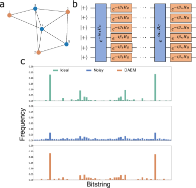
Figure 4: QAOA. a. An instance of a graph for for the Max-cut problem. b. The variational ansatz for implementing QAOA algorithm. c. Ideal, Noisy and Mitigated frequency of measurement results.

QAOA Zhou et al. (2020) is a quantum algorithm specifically designed for solving combinatorial optimization problems. The core of this algorithm involves encoding the objective function of the target optimization problem into a Hamiltonian, and trains an elaborately designed parameterized circuit to approximate the ground state. The final solution is derived by sampling bitstrings from the circuit’s output in the computational basis. However, when running a well-trained QAOA circuit on noisy quantum computers, the resulting output distribution deviates from the ideal scenario, which results in less accurate solutions. Hence, our goal is to mitigate this noise-induced bias in the output distribution, thereby providing experimenters with more precise solutions.

In this specific application, we focus on implementing QAOA for the maximum cut (Max-cut) problem Guerreschi and Matsuura (2019). The goal is to find a bi-partition of a graph $G$, namely subsets $A$ and $B$, in which the partition contains the maximum number of edges. This can be defined as an optimization with objective

$$\max_{\bm{z}}L(\bm{z})=\frac{1}{2}\sum_{(i,j)\in E}(1-z_{i}z_{j}),$$ (4)

where $i$, $j$ denote the indices of vertices, $(i,j)$ represents the edge connecting vertex $i$ and vertex $j$, and $E$ is the set containing all edges of the graph. If vertex $i$ belongs to subset $A$, then $z_{j}=1$, otherwise $z_{j}=0$. We provide an instance of $G$ with 6 vertices in Figure. 4a. The corresponding Hamiltonian of this problem in QAOA can be described by the following:

$$H_{C}=\frac{1}{2}\sum_{(i,j)\in E}(I-Z_{i}Z_{j}),$$ (5)

where $Z$ is Pauli-Z operator. The circuit for QAOA, shown in Figure 4b, typically comprises two sets of parameterized quantum gates, alternating between a mixing operator $H_{B}=\sum_{n=1}^{N}\sigma^{x}_{n}$ and the problem-specific cost operator $H_{C}$. In Figure 4c, we present the mitigated results concerning the output state of a trained QAOA circuit applied to the graph depicted in Figure 4a. Here, we consider the depolarizing noise model and it can be described by

$$\rho\rightarrow(1-\lambda)\rho+\frac{\lambda}{4^{N}-1}\sum_{i}P_{i}\rho P_{i},$$ (6)

where $P_{i}$ are the $4^{N}-1$ Pauli gates excluding the identity gate. It’s evident that the mitigated frequency of measurement results closely approximates the ideal scenario, signifying that we can obtain more reliable solutions to the original Max-Cut problem through our DAEM model. It’s worth noting that both ZNE and CDR are designed specifically for mitigating errors in expectation values, and they cannot be applied directly to the probability distribution of measurement results, in contrast to our proposed DAEM.

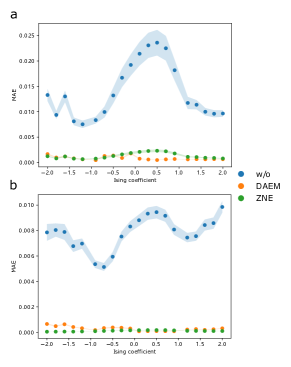
Figure 5: Spin-system dynamics. a.  Mean Absolute Errors (MAE) between the mitigated measurement expectation values for phase damping noise model and ideal expectation values. b. Mean Absolute Errors (MAE) between the mitigated measurement expectation values for amplitude damping noise model and ideal expectation values.

II.3 Error mitigation for spin-system dynamics

Our model works for quantum processes beyond the circuit model. It applies to, for example, the dynamics of physical systems. In this section, we delve into the challenge of error mitigation within the domain of spin-system dynamics, which is fundamental to various applications in quantum physics and materials science.

Here, our focus is on the dynamics of a 50-qubit quantum system with an Ising Hamiltonian $H_{\text{Ising}}$, descirbed in Eqn. 1. We consider the whole system’s evolution for time $t$, given as $U=\exp(-\textit{i}H_{\text{Ising}}t)$. This specific process is characterized by the following parameters: $J=1$, $g=2$, and a time duration of $t=5$. For the initial states involved in this Ising Hamiltonian evolution, we have selected the ground states of the Ising model, varying $J$ within the range $[-2,2]$, while keeping $g$ constant at $1$. To simulate these processes, we employ a combination of two powerful techniques: the density matrix renormalization group (DMRG) White (1992) and time-evolving block decimation (TEBD) White and Feiguin (2004); Daley et al. (2004). In this setup, noise is introduced after the completion of the unitary quantum process. Specifically, we evaluate our model’s performance under two distinct noise models: phase damping and amplitude damping channels. For the set of measurements $\mathcal{M}$, we also consider all two-qubit Pauli measurements on nearest-neighbor qubits. The results, corresponding to different values of $g$ in the input states, are presented in Figure 5. We can observe that both our model and ZNE have achieved nearly perfect mitigation, as evidenced by the MAE between the mitigated expectation values and the ground-truth values, which are close to zero. It is important to highlight that ZNE relies on precise knowledge of the noise levels corresponding to the noisy measurement data, whereas our DAEM model does not have this requirement. CDR is a technique tailored for quantum circuits, and therefore, it cannot be employed to mitigate errors in spin-system dynamics.

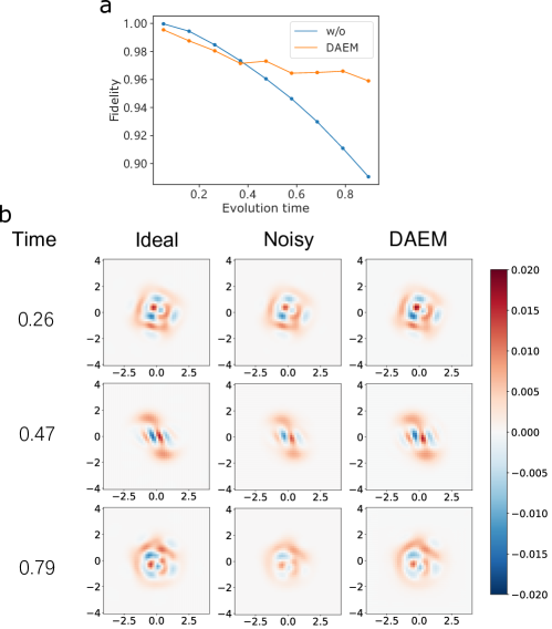
Figure 6: Continuous variable. a. Fidelity values between the noisy/mitigated state and the ideal state. b. Snapshots of the point-wise measurement results of the state at different time points.

II.4 Error mitigation for continuous-variable processes

Continuous-variable quantum systems have demonstrated their potential in diverse applications including quantum cryptography Jouguet et al. (2013) and quantum computing Lloyd and Braunstein (1999). However, despite the growing significance of this type of systems, no prior research has discussed the issue of error mitigation within continuous-variable quantum systems as far as we know. In this section, we applied our proposed DAEM model to address this long-unexplored challenge first.

We assess the effectiveness of our method on the dynamics induced by Kerr’s nonlinear interaction Dykman (2012) , which is important for continuous variable quantum computing Lloyd and Braunstein (1999). Consider a quantum system initially prepared in a coherent state $\ket{\alpha}$ and subjected to the Kerr Hamiltonian $H_{\rm kerr}=\pi\hat{a}^{\dagger\,2}\hat{a}^{2}$, where $\hat{a}$ and $\hat{a}^{\dagger}$ represent the annihilation and creation operators. In this scenario, we model the noisy process by a lossy open system, whose dynamics is described by the Lindblad master equation:

$$\dot{\rho}=-\text{i}[H_{\rm kerr},\rho]+\lambda\mathcal{D}(\hat{a})(\rho).$$ (7)

Here, $\mathcal{D}(\hat{a})(\rho):=\hat{a}\rho\hat{a}^{\dagger}-\frac{1}{2}(\rho\hat{a}^{\dagger}\hat{a}+\hat{a}^{\dagger}\hat{a}\rho)$, and $\lambda$ represents the loss rate. Our objective is to mitigate the errors in this process, making it closely resemble the ideal closed-system dynamics governed by Schrödinger’s equation with Hamiltonian $H_{\rm kerr}$. In this setting, we consider the measurement results associated with the point-wise Wigner function Lutterbach and Davidovich (1997); Bertet et al. (2002). In our numerical experiments, we initialize the state as coherent state $\ket{\alpha}$ with $\alpha=1.5$ and dimension $N=15$. We vary the evolution time over the interval $t\in[0,1]$, considering different loss rates $\lambda\in\{0.6,0.65,0.7,0.75,0.8\}$. To train the neural model within DAEM, we construct $\mathcal{N}_{\lambda}(\mathcal{F})=I$ by applying evolution of two inverse Hamiltonians, so that the overall effect to the input state is an identity operation. Details regarding the construction of this fiducial process are provided in the Methods. We assess the effectiveness of our DAEM by computing the fidelities between the mitigated states and their noiseless counterparts, employing the values of the point-wise Wigner function. As shown in the numerical results presented in Figure 6a, the fidelity between the state affected by the noise and the ideal state decreases rapidly as time increases. In contrast, our method excels in mitigating this effect, resulting in a dramatic improvement in fidelity. We also present snapshots of the state at different time points in Figure 6b, and our mitigated point-wise measurement results are notably closer to the ideal ones, particularly for longer evolution.

III Discussion

Distinguishing itself from previous quantum error mitigation methods, our proposed DAEM model exhibits a remarkable adaptability to various noise models and can be flexibly applied to a wide range of measurement settings. It shares similarities with ZNE in using measurement statistics corresponding to different noise levels, making it versatile. Meanwhile, it leverages the representational capability and adaptability of deep neural networks, allowing it to effectively handle complex noise scenarios. For instance, DAEM excels in dealing with the Non-Markovian noise model, illustrated in Figure 2e, where ZNE tends to perform poorly due to its reliance on a predefined extrapolation algorithm.

Furthermore, the subsequent CDR, while displaying some capability to adapt to different noise types, lacks robustness since it requires a classically simulable training circuit with a similar noise model to the target circuit. The effectiveness of CDR can vary significantly depending on how closely the training circuits matches the target circuit, which might not always be achievable in practical experiments. On the other hand, both ZNE and CDR are just proficient in mitigating measurement expectation values, but their extension to mitigate measurement probability distributions is challenging, restricting their applicability in quantum processes that involve obtaining the probability distribution of measurement results, as seen in the case of QAOA. As for another alternative method, called probabilistic error cancellation Temme et al. (2017); Endo et al. (2018); Van Den Berg et al. (2023), it estimates noise-free expectation values by representing them as linear combinations of expectation values from a set of noisy quantum circuits. However, this method requires gate tomography D’Ariano and Presti (2001) to accurately characterize the noisy gates, which involves exponential sample complexity. Accordingly, its applicability becomes challenging when extending to large-scale quantum systems due to the impractical computational demands.

In the future, our proposed DAEM model has the potential for extension to mitigate a broader range of realistic quantum errors, including crosstalk errors Ash-Saki et al. (2020); Sarovar et al. (2020). Crosstalk errors are prevalent in most multi-qubit quantum computing systems. Due to hardware imperfection, the assumption of locality and independence of quantum operations is usually violated in practice. Thus, a quantum gate can introduce unintended perturbations to its adjacent qubits, leading to crosstalk error. Modeling this non-local noise is challenging in practical scenarios Murali et al. (2020). However, given our framework does not require prior error modeling, it is a competitive candidate to handle this type of intricate noise.

For another, the majority of previous works have predominantly focused on quantum error mitigation of measurement expectations within quantum circuits, which restricts their utility across various quantum processes. Notably, there exist diverse quantum computation models Lloyd and Braunstein (1999); Gershenfeld and Chuang (1997) founded on quantum processes that extend beyond quantum circuits. Hence, the exploration of a comprehensive framework for addressing the problem of error mitigation in various quantum processes represents a pivotal undertaking, and in this study, we have taken the very first and substantial step towards achieving this goal.

Although previous efforts have delved into the utilization of artificial neural networks for quantum error mitigation Kim et al. (2020); Liao et al. (2023); Zhukov and Pogosov (2022); Sack and Egger (2023), their approaches primarily treats the neural model as a post-processing tool for the given data. In this study, we draw inspiration from the remarkable success of zero-shot learning Wang et al. (2019) and contrastive learning Chen et al. (2020) in classical machine learning, and apply the data augmentation technique in the design of our model for quantum error mitigation. Instead of adhering to a model-centric approach that focuses on finding the optimal model for a given dataset, our approach leverages the capabilities of data-centric AI (DCAI) strategies Ng et al. (2021) to seamlessly integrate the quantum process with the neural model. This paradigm shift redefines quantum error mitigation, moving from passive post-processing of collected measurement data to the active engagement of the quantum process during the error mitigation. This transformative data augmentation technique holds the potential to extend to other tasks in quantum information processing beyond error mitigation, including enhancing parameter estimation in quantum metrology Giovannetti et al. (2006). In a broader context, our work paves the way for the integration of advanced strategies from classical machine learning into solving crucial challenges on the path to achieving reliable quantum technologies.

IV Methods

IV.1 Neural Model in DAEM

Our error mitigation is model-agnostic thus the structure of the neural model can be flexibly chosen, ranging from simple linear models Hastie et al. (2001), multi-layer perceptrons (MLP) Haykin (1994), to deep neural networks like convolutional neural networks He et al. (2015) and Transformers Vaswani et al. (2017). In practice, we adopt a problem-aware strategy to design the specific construction of the model. In general, we prefer non-linear models for they have stronger ability to capture the intrinsic characteristics of various noise models.

For error mitigation in quantum algorithms and spin systems, we use MLP as the architecture of the neural model. The neural network is composed of multiple layers of fully connected neurons. Each neuron involves one linear transform followed by one non-linear activation. The stack of neurons allows for complex non-linear function fitting, which is powerful for estimating the expectation values and probability distributions in our error mitigation settings. The model’s inputs are parameter indicating the target circuit for mitigation, the observable to be measured, and the measurement statistics. The model’s output is either a real number or a probability distribution obtained by passing through a softmax function, depending on the measurement statistics to be mitigated. The cost function for mitigating expectation values is $L_{2}$ loss, namely

$$\mathcal{L}(\bm{y},\bm{y}_{\text{fid}})=\frac{1}{N}\sum_{i=1}^{N}(y^{(i)}-y_{\text{fid}}^{(i)})^{2},$$ (8)

where $\bm{y}$ denotes the output of the neural model and $\bm{y}_{\text{fid}}$ are the observable expectation values generated from data augmentation using fiducial channel. The cost function for mitigating probability distribution is the average relative entropy Cover and Thomas (2006), defined as

$$\mathcal{L}(\bm{p},\bm{p}_{\text{fid}})=\frac{1}{N}\sum_{i=1}^{N}\sum_{x}p^{(i)}(x)\log\left(\frac{p^{(i)}(x)}{p^{(i)}_{\text{fid}}(x)}\right),$$ (9)

where $\bm{p}$ are probability distribution predicted by our model, and $\bm{p}_{\text{fid}}$ are distribution obtained from fiducial channel by sampling 10000 shots.

To mitigate errors in continuous-variable processes, we adopt U-Net Ronneberger et al. (2015), a convolutional neural network originally designed for image segmentation Minaee et al. (2022), to be the neural model denoising the 2-dimensional Wigner function. U-Net possesses the strong ability to extract spatial features and construct 2-dimensional distributions. In this sense, it is helpful for learning the distribution of the point-wise Wigner function. The inputs to the model are evolution time and Wigner functions corresponding to different photon loss rates. The output is a single 2-dimensional feature map, which represents the denoised Wigner function. To train the neural model, we use $L_{1}$ loss as cost function, defined as

$$\mathcal{L}(\bm{y},\bm{y}_{\text{fid}})=\frac{1}{N}\sum_{i=1}^{N}\left|y^{(i)}-y_{\text{fid}}^{(i)}\right|.$$ (10)

It encourages sparse output distribution, which conforms to the Wigner quasiprobability distribution of our target states.

IV.2 Data augmentation strategy

Our data augmentation strategy enables training neural models to mitigate errors without noise-free statistics as labels. Since the goal of error mitigation is finding measurement statistics that is close to the noiseless ones, it is not proper to involve noiseless measurements of the target circuit in training. However, neural networks are too flexible due to their large amount of parameters, disabling their ability to extrapolate like ZNE. This shows that labels are necessary to guide neural networks to promising outputs.

In practice, the noise-free labels are no available unless we know the exact noiseless output states of the circuits. However, if the input and output states are the same in the noise-free scenario, we can directly measure the input states to generate labels. Here, we introduce a fiducial process, i.e., $\mathcal{N}_{\lambda}(\mathcal{F})$, to achieve this goal. The process is trivially identity or contains only CNOT gates that can be absorbed into observables, but shares the same noise as the target circuit. Specifically, the training set for Noise-Awareness phase is generated by feeding input states to the fiducial process, measuring noisy outputs as data and measuring the original inputs as labels. Note that the inputs can be either noisy or noiseless. We call this procedure data augmentation because labels comes naturally from not simulators but the input states themselves, which resembles the classical data augmentation like image transformations that enlarges the dataset without efforts to annotate new labels, because labels come from the original images. We detail the choice of input states and specification of $\mathcal{N}_{\lambda}(\mathcal{F})$ for different applications as follows.

Swap test

For swap test circuits, the states to be compared are pure states. In Noise-Awarenes phase, we sample 170 random pairs of pure states from Haar measure, in which 100 are used for training, 50 for validation and 20 left for Error-Mitigation phase. For ancilla, we choose random single-qubit mixed states. We construct the fiducial process by replacing every single-qubit gate by identity gate, leaving the CNOT gates unchanged. This results in a channel $\mathcal{N}_{0}(\mathcal{F})=U$, in which $U$ describes the effects of all CNOT gates in the original circuit. Then we excute the fiducial process in noisy environment with varying noise levels, and measure the noisy outputs using observable $M=Z_{1}$, which denotes the Pauli-Z observable on the ancilla qubit, and calculate the expectation values. Meanwhile, we measure the input states with observable $\tilde{M}=U^{\dagger}Z_{1}U$. The resulting expectation values are the corresponding labels.

Variational quantum eigensolvers

In VQEs, the augmentation strategy is generally the same as in Swap test. One difference is that, rather than pure states, we randomly sample 100 mixed states as inputs in the Noise-Awareness phase. Whereas in the Error-Mitigation phase, the input states are chosen to be ground state $|0\rangle$.

Quantum approximate optimization algorithms

For QAOA circuits, we found the distributions of output bitstrings possess symmetry, e.g., if 00011 is one solution, 11100 should also be a solution. In order to boost the performance of the neural model, we want to make the output distributions of the dataset in Noise-Awareness phase more aligned with those in the Error-Mitigation phase, i.e., the output distributions in training set also have this symmetry. It can be mathematically described as $X^{\otimes n}|\psi\rangle=|\psi\rangle$, where $X$ is Pauli-X operator. This shows that the input states $|\psi\rangle$ are the eigenvectors of $X^{\otimes n}$ with eigenvalue 1. In implementation, we sample 100 vectors from the eigenspace of $X^{\otimes n}$ with eigenvalue 1 as the input states. To generate fiducial process, after replacing all single-qubit gates by identity gates, the CNOT gate automatically cancels each other. In this case, the fiducial process is trivially identity, i.e., $\mathcal{N}_{0}(\mathcal{F})=I$. Again, we execute the fiducial process on noisy quantum devices with different noise levels to acquire noisy bitstring distributions. Besides, we sample input states $|\psi\rangle$ in computational basis to obtain labels.

Spin systems

The input states in both Noise-Awareness phase and Error-Mitigation phase are sampled from the same distribution. We have 100 different states for training in the first phase and 20 for testing in the second phase. The fiducial process is constructed by simply setting $H_{\text{Ising}}=I$.

Continuous-variable processes

To generate initial states, we first record intermediate states during $H_{\text{kerr}}$ noisy evolution in the time interval $t\in[0,1]$, each with timestep 0.05. With this procedure, we obtain 20 noisy states. Next, for each state, we evolve it with fiducial process $\mathcal{N}_{0}(\mathcal{F})=I$ under different loss rates. The evolution times are uniformly chosen from $[0,1]$ with gap 0.1. Note the fiducial process is constructed by a forward evolution followed by a reverse evolution. Specifically, suppose the total evolution time is $t_{0}$. Then, for $t\leq t_{0}/2$, the state evolves with Hamiltonian $H_{\text{kerr}}$, and $-H_{\text{kerr}}$ for $t_{0}/2\leq t\leq t_{0}$. We highlight that this kind of evolution can be simulated on hardware by Rossini et al. (2023).

Acknowledgement. We thank Qiushi Liu, Ya-Dong Wu for the helpful discussions. This work is supported by the Guangdong Basic and Applied Basic Research Foundation (Project No. 2022A1515010340) and by the Hong Kong Research Grant Council (RGC) through the Early Career Scheme (ECS) grant 27310822 and the General Research Fund (GRF) grant 17303923. This work was supported by funding from the Hong Kong Research Grant Council through grants no. 17300918 and no. 17307520, through the Senior Research Fellowship Scheme SRFS2021-7S02, and the John Templeton Foundation through grant 62312, The Quantum Information Structure of Spacetime (qiss.fr). Research at the Perimeter Institute is supported by the Government of Canada through the Department of Innovation, Science and Economic Development Canada and by the Province of Ontario through the Ministry of Research, Innovation and Science. The opinions expressed in this publication are those of the authors and do not necessarily reflect the views of the John Templeton Foundation.

Note added. After the completion of this work, another work Babukhin (2023) appeared where a data generation technique is employed to mitigate errors in the transverse field Ising model. This approach can be viewed as a specific means of obtaining the fiducial process.

Appendix A Implementation details of DAEM

A.1 Dataset Construction

The algorithm for constructing dataset both in the Noise-Awareness phase and in Error-Mitigation phase is shown in Algorithm 1.

Data: indicator of the phase in DAEM $p$, the set of input states $\mathcal{S}$, observables $\mathcal{M}$, the target quantum processes $\mathcal{N}_{\lambda}(\mathcal{E})$, property of the target process $g$, noise levels $\lambda$, measurement statistics $m$.

Result: dataset $\mathcal{D}$.

Initialize $\mathcal{D}\leftarrow\emptyset$;

if $p=\text{Noise-Awareness phase}$ then

       Construct fiducial process $\mathcal{N}_{\lambda}(\mathcal{F})$;

       $\mathcal{N}_{\lambda}\leftarrow\mathcal{N}_{\lambda}(\mathcal{F})$;

      

else

       $\mathcal{N}_{\lambda}\leftarrow\mathcal{N}_{\lambda}(\mathcal{E})$;

      

end if

for each $\rho_{s}\in\mathcal{S}$ do

       for each $\bm{M}\in\mathcal{M}$ do

             // Construct data.

             $\bm{P}\leftarrow\emptyset$;

             for each $\lambda_{k}\in\lambda$ do

                   Pass the state $\rho_{s}$ into the quantum process $\mathcal{N}_{\lambda_{k}}$ and obtain the output state $\rho_{o}=\mathcal{N}_{\lambda_{k}}(\rho_{s})$;

                   if $m=\text{expectation value}$ then

                         Measure the output state $\rho_{o}$ with observable $\bm{M}$ and calculate the expectation value $\bm{p}=\operatorname{tr}(\bm{M}\rho_{o})$;

                        

                  else

                         Measure the output state $\rho_{o}$ with observable $\bm{M}$ obtain the output distribution of the bitstrings $\bm{p}$;

                        

                   end if

                  $\bm{P}\leftarrow\bm{P}\cup\{\bm{p}\}$;

                  

             end for

            // Construct labels.

             if $p=\text{Noise-Awareness phase}$ then

                   if $\mathcal{N}_{0}(\mathcal{F})\neq I$ then

                         $U\leftarrow\mathcal{N}_{0}(\mathcal{F})$;

                         $M_{0}\leftarrow U^{\dagger}\bm{M}U$;

                        

                  else

                         $M_{0}\leftarrow\bm{M}$;

                        

                   end if

                  Measure input state $\rho_{s}$ with observable $M_{0}$ and obtain the measurement statistics $\bm{p}_{0}$;

                  

            else

                   Simulate the ideal output state for evaluation $\rho_{i}=\mathcal{N}_{0}(\mathcal{E})$;

                   Measure output state $\rho_{i}$ with observable $\bm{M}$ and obtain the measurement statistics $\bm{p}_{0}$;

                  

             end if

            $\mathcal{D}\leftarrow\mathcal{D}\cup\{(g,\bm{M},\bm{P},\bm{p}_{0})\}$;

            

       end for

      

end for

Algorithm 1 Dataset construction for DAEM

In the Noise-Awareness phase, we generate input states $\mathcal{S}_{\text{NA}}\subset\mathcal{S}$ and fiducial process $\mathcal{N}_{\lambda}(\mathcal{F})$ as introduced in the main text. We choose 100 states for training and 50 for validation. The state $\rho_{s}$ is passed into the fiducial process with various noise levels $\{\lambda_{k}\}$ described in the main text. For each output state with noise level $\lambda_{k}$, we measure every adjacent qubits using all two-local Pauli obervables $\bm{M}_{i}\in\mathcal{M}$, and obtain the measurement statistics $\bm{p}^{k}_{is}$. Note that in the continuous variable experiment, the output is a Wigner quasi-probability distribution, which requires no observable for measurement, thus we set $\mathcal{M}=\{I\}$. The measurement statistics with different noise levels are collected and formed a vector $\bm{P}_{is}=\left(\bm{p}^{(1)}_{is},\dots,\bm{p}^{(K)}_{is}\right)$. Meanwhile, we note down the property of the target process as $g$. For VQE and spin system experiments, $g$ stands for the coefficient of the Hamiltonian. For QAOA and swap test experiments, $g$ is purely integer indicating individual process. For continuous variable process, $g$ is the evolution time of the state. Besides, to generate labels, we measure the input state $\rho_{s}$ and obtain the measurement statistics $\bm{p}^{(0)}_{is}$. After recording these data, we put them together to form the dataset $\mathcal{D}_{\text{NA}}=\left\{g_{i},\bm{M}_{i},\bm{P}_{is},\bm{p}^{(0)}_{is}\right\}$.

In Error-Mitigation phase, the selection of input states $\mathcal{S}_{\text{EM}}\subset\mathcal{S}$ and quantum process $\mathcal{N}_{\lambda}(\mathcal{E})$ conforms to the experiment settings. The state is passes through the quantum processes with the same noise levels as in the Noise-Awareness phase, and the output is measured using the same observables. The dataset is formed as $\mathcal{D}_{\text{EM}}=\left\{g_{i},\bm{M}_{i},\bm{P}_{is},\bm{p}^{(0)}_{is}\right\}$. Whereas here $\bm{p}^{(0)}_{is}$ is obtained by classical simulation, which is used only to evaluate the performance.

A.2 Neural model in DAEM

The neural model in DAEM is implemented using PyTorch Paszke et al. (2019) package. The specific structure of the neural model is determined by input data format. For mitigating errors in quanum algorithms and spin-system dynamics, we use multi-layer perceptron (MLP). For mitigating errors in continuous variable processes, we use a modified U-Net.

MLP

The MLP for mitigating errors in quantum algorithms and spin system dynamics consists of 1 embedding block and 4 layers of neurons. The dimensions of hidden layers are 512, 1024, 1024 respectively. Besides, the nonlinear activation in our implementation is Mish Misra (2020), an advanced activation function widely applied in modern neural network designs. The structure of the network is shown in Figure 7.

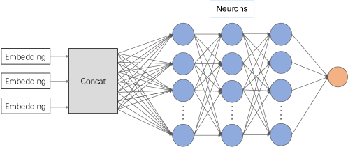
Figure 7: Structure of MLP used for mitigating errors in quantum algorithms and Spin-system dynamics.

The input of the network is $(g_{i},\bm{M}_{i},\bm{P}_{i})$. The embedding block maps the values of $g_{i}$, $\bm{P}_{i}$ into 128 dimensional vectors. For $M_{i}$, we separate the real and image part, concatenate them together and flatten the whole matrix into a vector. The vector is then transformed by the embedding block into a 128 dimensional vector. After embedding, the subsequent neurons takes the embedded vectors as input and outputs the mitigated measurements. The output of the network is the mitigated measurement statistics $\hat{\bm{p}}^{(0)}_{i}$.

For training, we use Adam Kingma and Ba (2017) as optimizer with initial learning rate 2e-4 and train for 300 epochs. The batch size is chosen to be 64. The training procedure follows the algorithm described in Algorithm 2.

Data: dataset $\mathcal{D}_{\text{NA}}$, number of epochs $E$, batch size $B$, neural model $f_{\bm{\theta}}$.

Result: Neural model $f_{\bm{\theta}}$ with trained parameters $\bm{\theta}$.

Initialize random parameters $\bm{\theta}$, $itr=0$;

while $itr<E$ do

       $\mathcal{D}\leftarrow\mathcal{D_{\text{NA}}}$;

       while $\mathcal{D}\neq\emptyset$ do

             Randomly sample $B$ unrepeated samples from the dataset $\bm{d}\sim\mathcal{D}_{\text{NA}}$;

             Separate the data $\bm{x}=\{g_{i},\bm{M}_{i},\bm{P}_{i}\}_{i=1}^{B}$ and labels $\bm{y}=\{\bm{p}^{(0)}_{i}\}_{i=1}^{B}$;

             Input data to the neural model and obtain predict results $\hat{\bm{p}}^{(0)}=f_{\bm{\theta}}(\bm{x})$;

             $\mathcal{D}\leftarrow\mathcal{D}\setminus{\bm{d}}$;

             Calculate the loss using the cost function according to the mitigation task as $l=\mathcal{L}(\hat{\bm{p}}^{(0)},\bm{y})$;

             Update the parameters of the model using Adam optimizer $\bm{\theta}\leftarrow\bm{\theta}-\text{Adam}\left(\nabla_{\bm{\theta}}l\right)$;

            

       end while

      $itr\leftarrow itr+1$;

      

end while

Algorithm 2 Training of neural model in Noise-Awareness phase.

U-Net

The U-Net used in the continuous variable experiment is a modified implementation of the standard U-Net in Ronneberger et al. (2015), as shown in Figure 8.

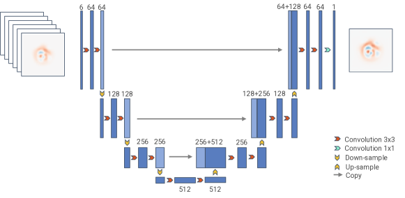
Figure 8: Structure of U-Net used for mitigating errors in continuous-variable processes.

The network contains one embedding block, 3 down-sample blocks, 3 up-sample blocks and 1 output layer. Specifically, one down-sample block contains 2 convolution blocks and 1 MaxPooling Nagi et al. (2011) operation. Each convolution block is composed by 1 convolution operation O’Shea and Nash (2015), followed by 1 LeakyReLU Maas et al. (2013) and 1 BatchNorm Ioffe and Szegedy (2015). One up-sample block contains 2 convolution blocks and 1 Bilinear interpolation Gonzales and Wintz (1987). The input to the network is $(g_{i},\bm{P}_{i})$. $\bm{P}_{i}$ is a tensor of shape $5\times 48\times 48$, which corresponds to the Wigner quasi-probability distribution with 5 different noise levels. Before embedding, $g_{i}$ is repeated, reshaped into the shape of the Wigner quasi-probability distribution, and stacked with $\bm{P}_{i}$ to form a $6\times 48\times 48$ tensor. This tensor is sent into the embedding block of the network, which consists of two convolution blocks. The output layer is one convolution operation with kernel size 1 and Tanh activation. The output of the network $\hat{\bm{p}}^{(0)}_{i}$ is the mitigated Wigner function with shape $1\times 48\times 48$. We train the network for 300 epochs using Adam optimizer with initial learning rate 2e-4 and batch size 32. The training procedure is the same as in Algorithm 2.

Appendix B Simulation details

B.1 Non-markovian noise model

For non-markovian noise, we consider the case that each gate inside the circuit is assigned with an independent bath. The interaction between the gate and its bath is formulated by the Spin-Boson model Breuer and Petruccione (2007), which is described by the Hamiltonians

$$H =H_{S}+H_{B}+H_{SB},$$ (11)

$$H_{B} =\sum_{k}\omega_{k}b_{k}^{\dagger}b_{k},$$ (12)

$$H_{SB} =\sum_{k}\sigma_{z}\otimes(\lambda_{k}b_{k}+\lambda_{k}^{*}b_{k}^{\dagger}),$$ (13)

where $b_{k}$ is the annihilation operator for mode $k$, and $\omega_{k}$ is the corresponding energy. The system Hamiltonian $H_{S}$ is chosen according to the actual quantum gate. The bath can be characterized by the spectral density Breuer and Petruccione (2007), which is defined as

$$J(\omega)=|\lambda_{k}|^{2}\delta(\omega-\omega_{k}).$$ (14)

In our experiments, we consider the continuum bath with spectral density

$$J(\omega)=\alpha\omega_{c}^{1-s}\omega^{s}e^{-\omega/\omega_{c}},$$ (15)

where we set $\alpha=0.001$, $s=6$, and $\omega_{c}=5$. This corresponds to the situation that the system has weak coupling to the bath.

B.2 Simulation of quantum circuits

To allow for unified simulation of both Markovian and non-Markovian noise, we implemented a customized simulator. The simulator uses density matrix simulation strategy, and only support $\{R_{x},R_{z},\text{CNOT}\}$ as basis gates inside a circuit. All gates from an arbitrary circuits are first converted into these basis gates using the transpile function in Qiskit Qiskit contributors (2023). Next, the gates are further transformed into corresponding system Hamiltonians $H_{S}$ with evolution time associated with the gate parameters. For instance, if the gate inside the circuit is Pauli-X rotation, e.g., $R_{x}(\pi/4)$, then the corresponding system Hamiltonian is $H_{S}=X$, and the evolution time $t\propto\pi/4$. For CNOT gate, its corresponding Hamiltonian is

$$H_{\text{CNOT}_{1,2}}=\frac{\pi}{4}(-Z_{1}I_{2}+Z_{1}X_{2}-I_{1}X_{2}),$$ (16)

as introduced in Rigetti and Devoret (2010), where index 1 denotes the control qubit and index 2 denotes the target qubit. The evolution time is $t_{0}\propto 1$.

For simulation, in noise-free case, the output state of a quantum gate described by $H_{S}$ is given as

$$\rho^{\prime}=e^{-iH_{S}t}\rho_{0},$$ (17)

where $\rho_{0}$ is the input state. Whereas in the noisy case, we solve the evolution in interaction picture, and convert back to Schrödinger picture Lidar (2020). The simulation of the evolution of quantum states is done by NumPy Harris et al. (2020) and SciPy Virtanen et al. (2020) with numerical integrations involving the density matrix.

B.3 Simulation of spin-system dynamics

The initial states are ground states of random Ising model, which are generated by the DMRG algorithm White (1992). The number of DMRG sweeps is set to be 2. The number of iterations of Lanczos method for diagonalization is 2, and the maximum dimension of Krylov space in superblock diagonalization is 4.

For simulating the dynamics, we use TEBD algorithm White and Feiguin (2004); Daley et al. (2004). We choose timestep $dt=2$, the maximum singular values for the Matrix Product State Bridgeman and Chubb (2017) to be 25. We truncate the singular values smaller than 1e-10.

The noise is added at the end of the simulation, before measurement. This can be done by changing the observable and using the new observable for measurement. For example, consider a quantum state $\rho$ affected by quantum noise $\mathcal{E}$. This can be expressed using Kraus operators $\{K_{i}\}$,

$$\mathcal{E}(\rho)=\sum_{i}K_{i}\rho K_{i}^{\dagger}.$$ (18)

Measure the output by observable $M$, one obtains

$$\operatorname{tr}(M\mathcal{E}(\rho)) =\operatorname{tr}(M\sum_{i}K_{i}\rho K_{i}^{\dagger})$$ (19)

$$=\operatorname{tr}(\sum_{i}K_{i}^{\dagger}MK_{i}\rho)$$ (20)

$$=\operatorname{tr}(\tilde{M}\rho),$$ (21)

where $\tilde{M}=\sum_{i}K_{i}^{\dagger}MK_{i}$. Thus we can use this new observable to measure $\rho$, leading to the noisy measurement results.

B.4 Simulation of continuous-variable process

The initial state of the system is coherent state, defined as

$$|\alpha\rangle=e^{-\frac{|\alpha|^{2}}{2}}\sum_{n=0}^{\infty}\frac{\alpha^{n}}{\sqrt{n!}}|n\rangle,$$ (22)

which is expanded in the basis of Fock states $\{|n\rangle\}$. In our experiment, we choose $\alpha=1.5$ and truncate the number of Fock states in Hilbert space to be $N=15$. We simulate the continuous-variable process evolution using QuTiP package Johansson et al. (2012). We consider the Wigner function Lutterbach and Davidovich (1997); Bertet et al. (2002) of the state as measurement output, which is a 2-dimensional quasiprobability distribution. We quantize the distribution into $48\times 48$ grids, which is enough for describing the state.

Appendix C Implementation of error mitigation algorithms for comparative experiments

C.1 Zero-noise extrapolation

In our experiments, we use a quadratic function as extrapolation model to fit the noisy measurement data. The data is the same as in our DAEM’s input. Note that ZNE requires the exact noise levels as input, so we provide this additional information, which is not necessary for our neural model. For each different cirucit structure, observable, and initial state, we fit an individual ZNE model using the corresponding measurement data, and extrapolate to zero noise to obtain the mitigated result.

C.2 Clifford data regression

Clifford data regression in our experiments is implemented by fitting a linear model with random Clifford data. Specifically, for a target circuit and target observable to be mitigated, we generate 100 different Clifford circuits by replacing the single-qubit gates in the target circuit with random Clifford gates, while the CNOT gates are left unchanged. The Clifford data is generated by measuring the noisy Clifford circuits using the target observables, and classically simulating the corresponding noise-free measurements. We train the linear model with the generated Clifford data until convergence. Then we apply the trained model to mitigate errors. Note that for each different circuit and observable, individual Clifford data is generated to train the model.

References

- Cai et al. (2022) Zhenyu Cai, Ryan Babbush, Simon C Benjamin, Suguru Endo, William J Huggins, Ying Li, Jarrod R McClean, and Thomas E O’Brien, “Quantum error mitigation,” arXiv preprint arXiv:2210.00921 (2022).
- Temme et al. (2017) Kristan Temme, Sergey Bravyi, and Jay M Gambetta, “Error mitigation for short-depth quantum circuits,” Physical review letters 119, 180509 (2017).
- Li and Benjamin (2017) Ying Li and Simon C Benjamin, “Efficient variational quantum simulator incorporating active error minimization,” Physical Review X 7, 021050 (2017).
- Kandala et al. (2019) Abhinav Kandala, Kristan Temme, Antonio D Córcoles, Antonio Mezzacapo, Jerry M Chow, and Jay M Gambetta, “Error mitigation extends the computational reach of a noisy quantum processor,” Nature 567, 491–495 (2019).
- Kim et al. (2023a) Youngseok Kim, Christopher J Wood, Theodore J Yoder, Seth T Merkel, Jay M Gambetta, Kristan Temme, and Abhinav Kandala, “Scalable error mitigation for noisy quantum circuits produces competitive expectation values,” Nature Physics , 1–8 (2023a).
- Kim et al. (2023b) Youngseok Kim, Andrew Eddins, Sajant Anand, Ken Wei, Ewout Berg, Sami Rosenblatt, Hasan Nayfeh, Yantao Wu, Michael Zaletel, Kristan Temme, and Abhinav Kandala, “Evidence for the utility of quantum computing before fault tolerance,” Nature 618, 500–505 (2023b).
- Czarnik et al. (2021) Piotr Czarnik, Andrew Arrasmith, Patrick J Coles, and Lukasz Cincio, “Error mitigation with clifford quantum-circuit data,” Quantum 5, 592 (2021).
- Czarnik et al. (2022) Piotr Czarnik, Michael McKerns, Andrew T. Sornborger, and Lukasz Cincio, “Improving the efficiency of learning-based error mitigation,” (2022), arXiv:2204.07109 [quant-ph] .
- Strikis et al. (2021) Armands Strikis, Dayue Qin, Yanzhu Chen, Simon C Benjamin, and Ying Li, “Learning-based quantum error mitigation,” PRX Quantum 2, 040330 (2021).
- Lowe et al. (2021) Angus Lowe, Max Hunter Gordon, Piotr Czarnik, Andrew Arrasmith, Patrick J. Coles, and Lukasz Cincio, “Unified approach to data-driven quantum error mitigation,” Physical Review Research 3 (2021), 10.1103/physrevresearch.3.033098.
- Endo et al. (2018) Suguru Endo, Simon C Benjamin, and Ying Li, “Practical quantum error mitigation for near-future applications,” Physical Review X 8, 031027 (2018).
- Van Den Berg et al. (2023) Ewout Van Den Berg, Zlatko K Minev, Abhinav Kandala, and Kristan Temme, “Probabilistic error cancellation with sparse pauli–lindblad models on noisy quantum processors,” Nature Physics , 1–6 (2023).
- Huggins et al. (2021) William J. Huggins, Sam McArdle, Thomas E. O’Brien, Joonho Lee, Nicholas C. Rubin, Sergio Boixo, K. Birgitta Whaley, Ryan Babbush, and Jarrod R. McClean, “Virtual distillation for quantum error mitigation,” Phys. Rev. X 11, 041036 (2021).
- Koczor (2021) Bálint Koczor, “Exponential error suppression for near-term quantum devices,” Phys. Rev. X 11, 031057 (2021).
- Seif et al. (2023) Alireza Seif, Ze-Pei Cian, Sisi Zhou, Senrui Chen, and Liang Jiang, “Shadow distillation: Quantum error mitigation with classical shadows for near-term quantum processors,” PRX Quantum 4, 010303 (2023).
- Torlai et al. (2018) Giacomo Torlai, Guglielmo Mazzola, Juan Carrasquilla, Matthias Troyer, Roger Melko, and Giuseppe Carleo, “Neural-network quantum state tomography,” Nature Physics 14, 447–450 (2018).
- Zhu et al. (2022) Yan Zhu, Ya-Dong Wu, Ge Bai, Dong-Sheng Wang, Yuexuan Wang, and Giulio Chiribella, “Flexible learning of quantum states with generative query neural networks,” Nature Communications 13, 6222 (2022).
- Wu et al. (2023) Ya-Dong Wu, Yan Zhu, Ge Bai, Yuexuan Wang, and Giulio Chiribella, “Quantum similarity testing with convolutional neural networks,” Physical Review Letters 130, 210601 (2023).
- Bennewitz et al. (2022) Elizabeth R Bennewitz, Florian Hopfmueller, Bohdan Kulchytskyy, Juan Carrasquilla, and Pooya Ronagh, “Neural error mitigation of near-term quantum simulations,” Nature Machine Intelligence 4, 618–624 (2022).
- Kim et al. (2020) Changjun Kim, Kyungdeock Daniel Park, and June-Koo Rhee, “Quantum error mitigation with artificial neural network,” IEEE Access 8, 188853–188860 (2020).
- Liao et al. (2023) Haoran Liao, Derek S. Wang, Iskandar Sitdikov, Ciro Salcedo, Alireza Seif, and Zlatko K. Minev, “Machine learning for practical quantum error mitigation,” (2023), arXiv:2309.17368 [quant-ph] .
- Zhukov and Pogosov (2022) Andrey Zhukov and Walter Pogosov, “Quantum error reduction with deep neural network applied at the post-processing stage,” Quantum Information Processing 21 (2022), 10.1007/s11128-022-03433-9.
- Sack and Egger (2023) Stefan H. Sack and Daniel J. Egger, “Large-scale quantum approximate optimization on non-planar graphs with machine learning noise mitigation,” (2023), arXiv:2307.14427 [quant-ph] .
- Shorten and Khoshgoftaar (2019) Connor Shorten and Taghi M Khoshgoftaar, “A survey on image data augmentation for deep learning,” Journal of big data 6, 1–48 (2019).
- Taylor and Nitschke (2018) Luke Taylor and Geoff Nitschke, “Improving deep learning with generic data augmentation,” in 2018 IEEE symposium series on computational intelligence (SSCI) (IEEE, 2018) pp. 1542–1547.
- Wang et al. (2020) Yaqing Wang, Quanming Yao, James T Kwok, and Lionel M Ni, “Generalizing from a few examples: A survey on few-shot learning,” ACM computing surveys (csur) 53, 1–34 (2020).
- Wang et al. (2019) Wei Wang, Vincent W Zheng, Han Yu, and Chunyan Miao, “A survey of zero-shot learning: Settings, methods, and applications,” ACM Transactions on Intelligent Systems and Technology (TIST) 10, 1–37 (2019).
- Peruzzo et al. (2014) Alberto Peruzzo, Jarrod McClean, Peter Shadbolt, Man-Hong Yung, Xiao-Qi Zhou, Peter J Love, Alán Aspuru-Guzik, and Jeremy L O’brien, “A variational eigenvalue solver on a photonic quantum processor,” Nature communications 5, 4213 (2014).
- Buhrman et al. (2001) Harry Buhrman, Richard Cleve, John Watrous, and Ronald De Wolf, “Quantum fingerprinting,” Physical Review Letters 87, 167902 (2001).
- Farhi et al. (2014) Edward Farhi, Jeffrey Goldstone, and Sam Gutmann, “A quantum approximate optimization algorithm,” arXiv preprint arXiv:1411.4028 (2014).
- White et al. (2020) G. A. L. White, C. D. Hill, F. A. Pollock, L. C. L. Hollenberg, and K. Modi, “Demonstration of non-markovian process characterisation and control on a quantum processor,” Nature Communications 11 (2020), 10.1038/s41467-020-20113-3.
- Agarwal et al. (2023) Abhishek Agarwal, Lachlan P. Lindoy, Deep Lall, Francois Jamet, and Ivan Rungger, “Modelling non-markovian noise in driven superconducting qubits,” (2023), arXiv:2306.13021 [quant-ph] .
- Groszkowski et al. (2023) Peter Groszkowski, Alireza Seif, Jens Koch, and A. A. Clerk, “Simple master equations for describing driven systems subject to classical non-markovian noise,” Quantum 7, 972 (2023).
- Breuer and Petruccione (2007) Heinz-Peter Breuer and Francesco Petruccione, The Theory of Open Quantum Systems (Oxford University Press, 2007).
- Magazzù et al. (2018) L. Magazzù, P. Forn-Díaz, R. Belyansky, J.-L. Orgiazzi, M. A. Yurtalan, M. R. Otto, A. Lupascu, C. M. Wilson, and M. Grifoni, “Probing the strongly driven spin-boson model in a superconducting quantum circuit,” Nature Communications 9 (2018), 10.1038/s41467-018-03626-w.
- Zhou et al. (2020) Leo Zhou, Sheng-Tao Wang, Soonwon Choi, Hannes Pichler, and Mikhail D Lukin, “Quantum approximate optimization algorithm: Performance, mechanism, and implementation on near-term devices,” Physical Review X 10, 021067 (2020).
- Guerreschi and Matsuura (2019) Gian Giacomo Guerreschi and Anne Y Matsuura, “Qaoa for max-cut requires hundreds of qubits for quantum speed-up,” Scientific reports 9, 6903 (2019).
- White (1992) Steven R White, “Density matrix formulation for quantum renormalization groups,” Physical review letters 69, 2863 (1992).
- White and Feiguin (2004) Steven R White and Adrian E Feiguin, “Real-time evolution using the density matrix renormalization group,” Physical review letters 93, 076401 (2004).
- Daley et al. (2004) Andrew John Daley, Corinna Kollath, Ulrich Schollwöck, and Guifré Vidal, “Time-dependent density-matrix renormalization-group using adaptive effective hilbert spaces,” Journal of Statistical Mechanics: Theory and Experiment 2004, P04005 (2004).
- Jouguet et al. (2013) Paul Jouguet, Sébastien Kunz-Jacques, Anthony Leverrier, Philippe Grangier, and Eleni Diamanti, “Experimental demonstration of long-distance continuous-variable quantum key distribution,” Nature photonics 7, 378–381 (2013).
- Lloyd and Braunstein (1999) Seth Lloyd and Samuel L Braunstein, “Quantum computation over continuous variables,” Physical Review Letters 82, 1784 (1999).
- Dykman (2012) Mark Dykman, Fluctuating nonlinear oscillators: from nanomechanics to quantum superconducting circuits (Oxford University Press, 2012).
- Lutterbach and Davidovich (1997) L. G. Lutterbach and L. Davidovich, “Method for direct measurement of the wigner function in cavity qed and ion traps,” Phys. Rev. Lett. 78, 2547–2550 (1997).
- Bertet et al. (2002) P. Bertet, A. Auffeves, P. Maioli, S. Osnaghi, T. Meunier, M. Brune, J. M. Raimond, and S. Haroche, “Direct measurement of the wigner function of a one-photon fock state in a cavity,” Phys. Rev. Lett. 89, 200402 (2002).
- D’Ariano and Presti (2001) GM D’Ariano and P Lo Presti, “Quantum tomography for measuring experimentally the matrix elements of an arbitrary quantum operation,” Physical review letters 86, 4195 (2001).
- Ash-Saki et al. (2020) Abdullah Ash-Saki, Mahabubul Alam, and Swaroop Ghosh, “Experimental characterization, modeling, and analysis of crosstalk in a quantum computer,” IEEE Transactions on Quantum Engineering 1, 1–6 (2020).
- Sarovar et al. (2020) Mohan Sarovar, Timothy Proctor, Kenneth Rudinger, Kevin Young, Erik Nielsen, and Robin Blume-Kohout, “Detecting crosstalk errors in quantum information processors,” Quantum 4, 321 (2020).
- Murali et al. (2020) Prakash Murali, David C. Mckay, Margaret Martonosi, and Ali Javadi-Abhari, “Software mitigation of crosstalk on noisy intermediate-scale quantum computers,” in Proceedings of the Twenty-Fifth International Conference on Architectural Support for Programming Languages and Operating Systems, ASPLOS ’20 (Association for Computing Machinery, New York, NY, USA, 2020) p. 1001–1016.
- Gershenfeld and Chuang (1997) Neil A Gershenfeld and Isaac L Chuang, “Bulk spin-resonance quantum computation,” science 275, 350–356 (1997).
- Chen et al. (2020) Ting Chen, Simon Kornblith, Mohammad Norouzi, and Geoffrey Hinton, “A simple framework for contrastive learning of visual representations,” in International conference on machine learning (PMLR, 2020) pp. 1597–1607.
- Ng et al. (2021) Andrew Ng, Dillon Laird, and Lynn He, “Data-centric ai competition,” DeepLearning AI. Available online: https://https-deeplearning-ai. github. io/data-centric-comp/(accessed on 9 December 2021) (2021).
- Giovannetti et al. (2006) Vittorio Giovannetti, Seth Lloyd, and Lorenzo Maccone, “Quantum metrology,” Physical review letters 96, 010401 (2006).
- Hastie et al. (2001) Trevor Hastie, Robert Tibshirani, and Jerome Friedman, The Elements of Statistical Learning, Springer Series in Statistics (Springer New York Inc., New York, NY, USA, 2001).
- Haykin (1994) Simon Haykin, Neural networks: a comprehensive foundation (Prentice Hall PTR, 1994).
- He et al. (2015) Kaiming He, Xiangyu Zhang, Shaoqing Ren, and Jian Sun, “Deep residual learning for image recognition,” (2015), arXiv:1512.03385 [cs.CV] .
- Vaswani et al. (2017) Ashish Vaswani, Noam Shazeer, Niki Parmar, Jakob Uszkoreit, Llion Jones, Aidan N. Gomez, Łukasz Kaiser, and Illia Polosukhin, “Attention is all you need,” in Proceedings of the 31st International Conference on Neural Information Processing Systems, NIPS’17 (Curran Associates Inc., Red Hook, NY, USA, 2017) p. 6000–6010.
- Cover and Thomas (2006) Thomas M. Cover and Joy A. Thomas, Elements of Information Theory (Wiley Series in Telecommunications and Signal Processing) (Wiley-Interscience, USA, 2006).
- Ronneberger et al. (2015) Olaf Ronneberger, Philipp Fischer, and Thomas Brox, “U-net: Convolutional networks for biomedical image segmentation,” (2015), arXiv:1505.04597 [cs.CV] .
- Minaee et al. (2022) Shervin Minaee, Yuri Boykov, Fatih Porikli, Antonio Plaza, Nasser Kehtarnavaz, and Demetri Terzopoulos, “Image segmentation using deep learning: A survey,” IEEE Transactions on Pattern Analysis and Machine Intelligence 44, 3523–3542 (2022).
- Rossini et al. (2023) Mirko Rossini, Dominik Maile, Joachim Ankerhold, and Brecht I. C. Donvil, “Single-qubit error mitigation by simulating non-markovian dynamics,” Phys. Rev. Lett. 131, 110603 (2023).
- Babukhin (2023) D.V. Babukhin, “Echo-evolution data generation for quantum error mitigation via neural networks,” arXiv preprint arXiv:2311.00487 (2023).
- Paszke et al. (2019) Adam Paszke, Sam Gross, Francisco Massa, Adam Lerer, James Bradbury, Gregory Chanan, Trevor Killeen, Zeming Lin, Natalia Gimelshein, Luca Antiga, Alban Desmaison, Andreas Köpf, Edward Yang, Zach DeVito, Martin Raison, Alykhan Tejani, Sasank Chilamkurthy, Benoit Steiner, Lu Fang, Junjie Bai, and Soumith Chintala, “Pytorch: An imperative style, high-performance deep learning library,” (2019), arXiv:1912.01703 [cs.LG] .
- Misra (2020) Diganta Misra, “Mish: A self regularized non-monotonic activation function,” (2020), arXiv:1908.08681 [cs.LG] .
- Kingma and Ba (2017) Diederik P. Kingma and Jimmy Ba, “Adam: A method for stochastic optimization,” (2017), arXiv:1412.6980 [cs.LG] .
- Nagi et al. (2011) Jawad Nagi, Frederick Ducatelle, Gianni A. Di Caro, Dan Cireşan, Ueli Meier, Alessandro Giusti, Farrukh Nagi, Jürgen Schmidhuber, and Luca Maria Gambardella, “Max-pooling convolutional neural networks for vision-based hand gesture recognition,” in 2011 IEEE International Conference on Signal and Image Processing Applications (ICSIPA) (2011) pp. 342–347.
- O’Shea and Nash (2015) Keiron O’Shea and Ryan Nash, “An introduction to convolutional neural networks,” (2015), arXiv:1511.08458 [cs.NE] .
- Maas et al. (2013) Andrew L Maas, Awni Y Hannun, Andrew Y Ng, et al., “Rectifier nonlinearities improve neural network acoustic models,” in Proc. icml, Vol. 30 (Atlanta, GA, 2013) p. 3.
- Ioffe and Szegedy (2015) Sergey Ioffe and Christian Szegedy, “Batch normalization: Accelerating deep network training by reducing internal covariate shift,” (2015), arXiv:1502.03167 [cs.LG] .
- Gonzales and Wintz (1987) Rafael C Gonzales and Paul Wintz, Digital image processing (Addison-Wesley Longman Publishing Co., Inc., 1987).
- Qiskit contributors (2023) Qiskit contributors, “Qiskit: An open-source framework for quantum computing,” (2023).
- Rigetti and Devoret (2010) Chad Rigetti and Michel Devoret, “Fully microwave-tunable universal gates in superconducting qubits with linear couplings and fixed transition frequencies,” Phys. Rev. B 81, 134507 (2010).
- Lidar (2020) Daniel A. Lidar, “Lecture notes on the theory of open quantum systems,” (2020), arXiv:1902.00967 [quant-ph] .
- Harris et al. (2020) Charles R. Harris, K. Jarrod Millman, Stéfan J van der Walt, Ralf Gommers, Pauli Virtanen, David Cournapeau, Eric Wieser, Julian Taylor, Sebastian Berg, Nathaniel J. Smith, Robert Kern, Matti Picus, Stephan Hoyer, Marten H. van Kerkwijk, Matthew Brett, Allan Haldane, Jaime Fernández del Río, Mark Wiebe, Pearu Peterson, Pierre Gérard-Marchant, Kevin Sheppard, Tyler Reddy, Warren Weckesser, Hameer Abbasi, Christoph Gohlke, and Travis E. Oliphant, “Array programming with NumPy,” Nature 585, 357–362 (2020).
- Virtanen et al. (2020) Pauli Virtanen, Ralf Gommers, Travis E. Oliphant, Matt Haberland, Tyler Reddy, David Cournapeau, Evgeni Burovski, Pearu Peterson, Warren Weckesser, Jonathan Bright, Stéfan J. van der Walt, Matthew Brett, Joshua Wilson, K. Jarrod Millman, Nikolay Mayorov, Andrew R. J. Nelson, Eric Jones, Robert Kern, Eric Larson, C J Carey, İlhan Polat, Yu Feng, Eric W. Moore, Jake VanderPlas, Denis Laxalde, Josef Perktold, Robert Cimrman, Ian Henriksen, E. A. Quintero, Charles R. Harris, Anne M. Archibald, Antônio H. Ribeiro, Fabian Pedregosa, Paul van Mulbregt, and SciPy 1.0 Contributors, “SciPy 1.0: Fundamental Algorithms for Scientific Computing in Python,” Nature Methods 17, 261–272 (2020).
- Bridgeman and Chubb (2017) Jacob C Bridgeman and Christopher T Chubb, “Hand-waving and interpretive dance: an introductory course on tensor networks,” Journal of Physics A: Mathematical and Theoretical 50, 223001 (2017).
- Johansson et al. (2012) J.R. Johansson, P.D. Nation, and Franco Nori, “Qutip: An open-source python framework for the dynamics of open quantum systems,” Computer Physics Communications 183, 1760–1772 (2012).