Parametric model for high-order harmonic generation with quantized fields
Abstract
A quantum optical model for the high-order harmonic generation is presented, in which both the exciting field and the high harmonic modes are quantized, while the target material appears via parameters only. As a consequence, the model is independent from the excited material system to a large extent, and allows us to focus on the properties of the electromagnetic fields. Technically, the Hamiltonian known for parametric down-conversion is adopted, where photons in the th harmonic mode are created in exchange of annihilating photons from the fundamental mode. In our treatment, initially the fundamental mode is in a coherent state corresponding to large photon numbers, while the high harmonic modes are in vacuum state. Due to the interaction, the latter modes get populated while the fundamental one loses photons. Analytical approximations are presented for the time evolution that are verified by numerically exact calculations. For multimode, finite bandwith excitation, the time dependence of the high-order harmonic radiation is also given.
I Introduction
Optical generation of high-order harmonics (HH) [1, 2] is a key process for the generation of ultrashort electromagnetic pulses [3]. It is a strong-field phenomenon, in which the nonlinear material response leads to the emission of radiation with frequencies close to the integer multiples of the central frequency of the excitation. The effect has been demonstrated using various material samples [1, 2, 4, 5, 6, 7], and although the details are different, the exciting field is always orders of magnitude stronger than the harmonics. Therefore, besides the traditional models [8, 9] for high-order harmonic generation (HHG), quantized description (photon picture) is also of interest. Interestingly, observable signatures of the back-action of the HH modes on the photon statistics of the fundamental one have recently been demonstrated experimentally [10, 11]. This underlines the significance of field quantization during the process of HHG.
Considering the quantized description of strong-field effects, early theoretical models date back to the ’80s [12, 13]. In this framework, Ref. [12] provides the first non-perturbative treatment of HHG in the nonlinear Compton process. For HHG with atomic samples, Volkov states and transitions between them have also been considered [14, 15]. More recently, theoretical models in Refs. [16, 11] provide a background for the corresponding experimental findings reported in Refs. [10, 11]. The emergence of HHG spectra as the expectation value of the photon numbers in the HH modes were demonstrated in [17, 18, 19, 20], and a phase space description of the problem was given in Ref. [21]. Explicitly nonclassical features of the HH emission have been predicted also for realistic systems [22], and the consequences of excitation with quantum light have also been investigated [23]. For a recent tutorial on strong-field quantum electrodynamics, see Ref. [24].
The complete problem, i.e., considering both the excitation and the HH modes on the quantized level (with the material sample obviously treated quantum mechanically), raises numerical challenges. With reasonable approximations, either the HH modes [17], or the excitation [21] can be considered to be quantized, but it is demanding to solve a model, which assumes it for both fields. In order to focus on the most important quantum mechanical properties both of these fields, we have to use a model in which the number of different degrees of freedom is systematically decreased. This is indeed the aim of the current paper, in which, in a rather general way, the target material appears only via parameters – that can be fitted to the given material system in subsequent, more specific calculations.
II Model
The essence of high-order harmonic generation on the level of quantized fields is the creation of photons in the HH modes at the expense of decreasing the number of photons in the exciting (fundamental) modes. Clearly, in order to obtain a Hermitian Hamiltonian, we have to take the opposite process also into account. That is, by denoting the fundamental frequency by , we can write
| (1) | ||||
where are the annihilation (creation) operator of a mode with frequency while and belong to the fundamental mode. The coefficients are real numbers. The magnitude of these parameters is to be determined so as to reproduce experimental results, see in the next section and the Appendix.
The model proposed in Eq. (1) is clearly a simplification from various points of view. Obviously, the excitation is generally multi-mode, and has a finite duration. Similarly, the spectral widths of the high-order harmonics are also finite, and the HH peaks may not be positioned exactly at the integer multiples of (Specifically, for most samples, harmonics corresponding to even values of are missing, as we shall assume in the following.) Moreover, the dynamics of the electromagnetic modes (which can be obtained by ”tracing out” the degrees of freedom corresponding to the target material) can be more complex than the unitary time evolution induced by the Hamiltonian (1).
However, Eq. (1) – besides being instructive – clearly captures the most important features of the HHG process. Additionally, when only a single harmonic corresponding to is taken into account, (1) is identical to the Hamiltonian that is used for the description of parametric down-conversion (when the process is of interest [25]). That is, Eq. (1), with appropriate initial conditions, is closely related to the description of fundamental experiments related to photon pair creation [26, 27].
The natural initial condition for HHG is that the state of the fundamental mode (the mode that corresponds to an intense, practically classical radiation) is a coherent state, while the HH modes are in vacuum state:
| (2) |
where denotes the order of the highest harmonic that we take into account. In the following all the indices are considered to be odd, and we focus on the plateau region where the heights of the harmonic peaks are practically the same. This region is present for both gaseous and solid state target materials. In the power spectra, peaks that correspond to different harmonic frequencies and have equal heights mean the same amount of energy irradiated in the narrow spectral regions around the different frequencies In order to reproduce this effect in our model, the expectation values should be independent of . This can be achieved by choosing appropriate ratios of the parameters as we shall see in the next section.
III Parametric approximation
Since the intensity of the HH radiation is known to be orders of magnitude lower than that of the excitation, we can assume that the back-action of the HH modes on the fundamental one is weak. Therefore, as a first approximation, we can take the expectation value of Eq. (1) in the state which would be the result of the free time evolution of the fundamental mode [induced by the Hamiltonian ]. Using and the eigenvalue equation we obtain the following Hamiltonian in the parametric approximation:
| (3) |
where irrelevant additive constants have been omitted. (Note that this approximation is common for describing down-conversion [28]; its generalization to cases when the pump mode is not necessarily a coherent state can be found in Ref. [29].) As we can see, is a sum of independent terms, each of which can be treated separately. Thus, dropping the index for the moment, we are to consider the single mode Hamiltonian
| (4) |
where and
The time evolution induced by (4) can be solved using a systematic, standard way [30, 31]. However, it can be instructive to perform a direct calculation. To this end, we use the Heisenberg picture. The commutator leads to the following dynamical equation for the annihilation operator:
| (5) |
where denotes the identity operator, and the index refers to the Heisenberg picture. This equation can be solved:
| (6) |
Now let us use the time evolution operator, for which, with any initial state we have Clearly, where the explicit notation of the Schrödinger picture (the index ) has been introduced for clarity. Since we have
| (7) |
Returning to the Schrödinger picture, and using that we can write
| (8) |
That is, the time evolution starting from the vacuum state (which is the initial condition, see Eq. (2)) leads to a state that is an eigenstate of
| (9) |
This means that the state is a coherent state with the parameter of that is
| (10) |
Before analyzing this result, let us emphasize an important aspect that has experimental relevance as well. This is related to the phases of the various harmonics, which have to be locked relative to each other [3] in order that their superposition could lead to an isolated attosecond pulse, or a pulse train [32, 33]. Obviously, the phases of the coherent states (10) corresponding to different harmonics are linked via the common exciting state and consequently the same holds for the related electromagnetic field. Although at this point it can be seen as a consequence of the parametric approximation, our numerically exact calculations show that the relative phases of the different harmonics are practically constants at the initial stage of the time evolution.
As Eq. (10) implies, the photon number expectation value in the parametric approximation is given by
| (11) |
i.e., it is quadratic in . Clearly, it cannot hold for infinitely long times, which is a direct consequence of the approximation that the photon number expectation value of the fundamental mode is constant [34]. As we shall see in the next section, for physically realistic interaction times, this approximation is numerically proven to be acceptable. Additionally, Eq. (11) allows us to estimate the coefficients that lead to peaks in the power spectra with equal heights. The corresponding requirement is that is the same for all HH modes (c.f. the end of the previous section). Reintroducing the mode indices, and using Eq. (11), we see that
| (12) |
describes the ratio between the parameters that correspond to two different HH modes ( and ) in the plateau region. In view of this, the parameter
| (13) |
will be kept constant (independent of ) in the following in order to account for the plateau part of the spectrum. (A different choice for the parameters that corresponds to actual experimental data will be given in Appendix B.)
Note that the plateau condition that led to Eq. (13) can be too strong in the sense that it is based on an approximation, and the exact time evolution can be slightly different (see the next section). Additionally, for pulsed excitation, the HH photons are collected during the whole process, and the condition of having HH peaks with equal heights is to be fulfilled only at the end of the process. Fitting the parameters to different target materials may also slightly modify the condition (13). However, at the general level of the current work, this is a reasonable approximation.
The results to follow will be presented using the Schrödinger picture, without explicit notations (there will be no index from now on). Before turning to the numerical results, let us consider the case of multimode excitation within the framework above. We assume a pulsed-like excitation and for the sake of simplicity we consider discrete frequencies. As before, we restrict ourselves to the linearly polarized case. This means that we assume a (large) quantization volume in which the electromagnetic field with the given polarization direction can be written as a sum of contributions of modes with discrete frequencies. In Eq. (1) we took only a very limited number of modes into account, but in order to describe a pulsed-like excitation, even in free space, we need all the modes within the spectral range of the excitation. Let us consider the multimode exciting coherent state
| (14) |
where the frequencies corresponding to – to be denoted by – fall in the range . Knowing e.g., the experimentally available ”waveform” of the exciting electric field, the complex parameters can be chosen such that without any interaction, the expectation value of the quantum mechanical electric field operator, is the same as
In more detail, considering alone (”free space”) we have thus the expectation value is given by , and consequently we are essentially to determine the Fourier components of to obtain the required values. Alternatively, working in velocity gauge, the coefficients can be chosen so that the time evolution of the classical vector potential is reproduced by its quantum mechanical expectation value, ensuring that it holds also for both the electric and the magnetic fields.
Let us note that the mode expansion is usually considerably more complex than the one given – quite formally – by Eq. (14), even for a given polarization direction. E.g. the transversal structure of the modes and the mode density should also be taken into account for a detailed description. However, in order to see the approximate time evolution of the HH electric fields, we can consider Eq. (14) as the initial state for the modes corresponding to the exciting pulse. Using the free-space time evolution of the coherent states, we have:
| (15) | ||||
where the distribution of the frequencies are peaked around the fundamental one, i.e., and (recall that denotes the quantization volume). Now we use a further approximation, namely we assume that each harmonic state in the expansion (14) populates the corresponding HH modes (i.e., ) independently. (Clearly, depending on the mode density, it can be a strong simplification, thus the following results are to be considered in the qualitative sense.) According to Eq. (10), for the th harmonic we can write:
| (16) | ||||
where and correspond to the mode with frequency and, for the sake of simplicity, was considered to be constant in the frequency range
It is instructive to consider an example. For a pulse with Gaussian envelope, we have Since independently from by using Eq. (16), we obtain that the time dependence of is proportional to where the change of the carrier-envelope phase (CEP) () is a result of the factor in the coherent state .
When is compared to we see that there are obvious changes like replacing with and the times decrease of the pulse duration. The change of the CEP and the multiplicative factor of are, however, less trivial. It is important to emphasize that does not diverge in the long time limit, as a consequence of the presence of the Gaussian envelope, as That is, in the framework of the parametric approximation, a pulsed-like excitation leads to pulsed-like HH radiation, but the waveforms corresponding to the HH modes are not simply scaled copies of the exciting pulse.
IV Numerical results
It convenient to rewrite the time dependent Schrödinger equation using dimensionless time as
| (17) |
where the Hamiltonian is given by Eq. (1), and no additional approximations are used. Eq. (17) tells us that the independent parameters are Additionally, since the ”weighted photon number operator”
| (18) |
commutes with the problem is finite dimensional. More precisely, working in the photon number eigenbasis (for which and ), we see that for an initial state is the maximal index for the fundamental mode, and the photon numbers cannot exceed for the th harmonic mode either. As a consequence, for the physically interesting initial state given by Eq. (2), the only truncation in photon number eigenbasis is related to the representation of the initial coherent state (For nonzero the inner product is never zero exactly, but the photon number distribution is peaked around (see e.g. [28]) and the state can be estimated using a finite number of photon eigenstates with arbitrary precision.)
However, the difficulty of the numerical problem rapidly increases as we increase the number of modes that we take into account. The compromise between computation time and the requirement of accounting for different HH modes led us to consider two HH modes at a time, which allows us to take a few thousand exciting photons into account (i.e., ).
Clearly, the photon number operators and commute with the interaction-free Hamiltonian of the system . Therefore, when calculating the time evolution of the photon number expectation values, it is only the interaction term
| (19) |
that has to be considered, e.g.:
| (20) |
This means that it is only the relative magnitudes of the parameters that are essential. (In particular, if we take only a single HH mode () into account, the change does not change the time evolution of in a fundamental way, it only rescales the time variable ) Since – in order to reproduce the plateau region – the ratio of parameters are fixed [see Eq. (12)], the same scaling property applies to the general case. However, in order to be specific, in the following we will use that is, the unit of time will be (with denoting the exciting mode optical period). The parameter that is defined by Eq. (13) will also be given for the figures.
IV.1 The initial stage of the time evolution
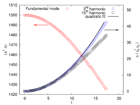
In the following, we present results obtained by solving the time dependent Schrödinger equation (17) numerically. The initial condition is given by Eq. (2), and we consider two HH modes. In order to see the behaviour of significantly different modes, we chose and The ratio is determined by Eq. (12). In this subsection we focus on the initial stage of the time evolution, in which (according to the previous section) the condition Eq. (12) should warrant that within a good approximation. As we can see in Fig. 1, indeed, this condition holds for small values of and even at the end of the considered time interval, the relative difference is below 20 %. Clearly, this difference is a consequence of the decreasing number of photons in the exciting mode, which corresponds to the gradual loss of the validity of the parametric approximation. Since the parameter of the coherent state corresponding to the th harmonic contains the th power of , higher orders are more sensitive to this effect.
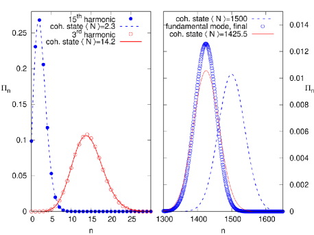
The decrease of the exciting intensity can also be seen in Fig. 2, where the numerically exact probability of having photons in a given mode (the photon statistics) is shown. As we can also see, the photon statistics are close to that of coherent states, especially considering the HH modes. (The deviation from the Poissonian statistics of a coherent state can be quantitatively analyzed using the Mandel parameter, see the next subsection.) More precisely, the probability e.g. for the fundamental mode is given by
| (21) |
At this point it is not necessary, but later it will be useful to introduce the reduced density matrices. For the th mode, it is the trace of the projector over the modes different from E.g., for
| (22) |
Using this notation,
Focusing on a single mode, the time evolution is often best visualized in the phase space [35]. First, we can use the expectation values of the Hermitian quadrature operators
| (23) |
which, for localized states, coincides well with the motion of the center of the wave packet. (E.g., for a coherent state we can easily see that the expectation value of is the real (imaginary) part of .) However, in the general case these expectation values do not contain the complete quantum mechanical information that is available in a (reduced) density operator, On the contrary, the Wigner function is in a one-to-one correspondence with Using the photon number eigenstate expansion, is conveniently calculated as the expectation value of the Wigner operator [36, 37]:
| (24) |
where is the displacement operator, and denotes the parity. The function is obtained by utilizing the identities and together with the fact that can be expressed using an associated Laguerre function [28].
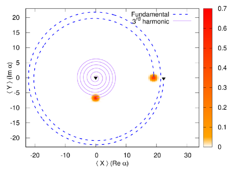
Fig. 3 summarizes the initial stage of the time evolution in phase space. (Note that in the context of parametric amplification [38, 39], a similar figure with functions appeared already in Ref. [38].) In order to maintain the clarity of the figure, we set For the third harmonic, the curve is a spiral which is well described by the real and imaginary parts of the complex number This supports the approximation that at this stage of the time evolution, the state of the HH modes are essentially the coherent states given by Eq. (10). The corresponding Wigner function is also very close to the Gaussian that corresponds to . This holds in spite of the fact that the exciting mode is not exactly the coherent state which is a direct consequence of losing photons that are upconverted to the HH mode.
However, the Wigner function that can be calculated using is still very close to a Gaussian. That is, in this stage of the time evolution the state of the exciting mode can be described well by a coherent state with an index the magnitude of which is decreasing.
IV.2 The complete dynamics
Considering the efficiency and typical duration of the HHG process, the relative number of exciting mode photons that are transferred to one of the HH modes is low, i.e., the photon number expectation value for the exciting mode is almost constant during the process. However, in order to complete the physical picture, it is instructive to investigate the time evolution on a considerably longer time scale.
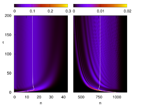
Fig. 4 shows the photon number distribution of the exciting mode and a single (the 15th) HH mode as a function of time. As we can see, the initially narrow (Poissonian) distribution first gets structured, multiple peaks appear, then these peaks become less pronounced, eventually approaching a wide distribution. Correspondingly, the expectation value of the photon number operators (solid white line in Fig. 4) converges to constant values. Note that the initial quadratic increase of is hardly visible in this figure, and similarly decreases approximately linearly till its minimum, and then a slow convergence towards a constant value starts. Clearly, since the expectation value of given by Eq. (18) is a constant of motion, is a (scaled) ”mirror image” of The positions and actual values of the extrema depends on which HH mode is investigated.
Explaining all the details of the complex dynamics shown in Fig. 4 requires a thorough analysis. Considering the qualitative behavior, the time evolution can be divided into two parts. The initial stage (till ) is quite intuitive, the photon distribution of the states remain localized (although super-Poissonian) and the dominant effect is the upconversion of exciting mode photons. However, since the number of these photons is finite, this process cannot last forever, and on the long timescale the flow of energy between the modes will be bidirectional. Thus the time evolution is analogous to the physical background of the ”collapse and revival” phenomena that are often investigated in the context of a two-level atom that exchanges energy with an exciting field which is initially in a coherent state [28]. In view of this, the fringes that can be seen in Fig. 4 correspond to the phenomenon of ”collapse”, when the eigenstates of the complete system gradually lose the relative phases that initially led to localized photon number distributions. Note that the result of this dephasing can be seen in Fig. 6 as well. Our numerical calculations also show that the discrete frequencies that correspond to the time evolution of the eigenstates later can rephase again (not shown in the picture). A similar ”revival” process was shown to appear during parametric down-conversion in Ref. [40].
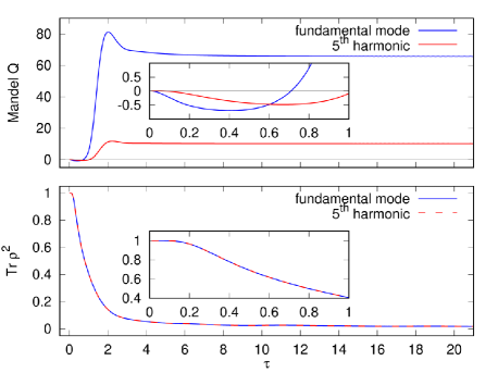
The difference of a photon number distribution from the Poissonian statistics is conveniently quantified using the Mandel parameter:
| (25) |
For a coherent state, while () corresponds to super-Poissonian (sub-Poissonian) distributions. The upper panel of Fig. 5 shows a typical example with the fundamental and the fifth HH mode. As we can see in the inset, at the initial stage of the time evolution for both modes (indications to this effect can be seen already in Fig. 2), but later on the variance of the photon numbers increases (in accord with Fig. 4), resulting in large positive values for
Note that both Fig. 5 and Fig. 4 suggest that the departure from the initial coherent state is faster for the fundamental mode than for the HH modes. This can be proven by a formal series expansion (see the Appendix), showing that for short times, is a quadratic function of time for the fundamental mode, while its first nontrivial order is only for the HH modes. This behavior can be used for further analytic approximations.
Finally, we discuss quantum entaglement between the field modes. Entanglement in strong-field and attosecond physics has obtained reviving attention in the past years [41], including also electon-ion [42, 43] and electron-electron entanglement [44]. The entanglement between our field modes is weak at the initial stage of the time evolution, since the state of the system is appropriately estimated by the tensor product of coherent states. This is visualized by the lower panel of Fig. 5, in which and are plotted as a function of time. (Note that since in this case there are only two modes, we should have which, as Fig. 5 shows, is true also in our numerical calculation.) As we can see, at the beginning of the time evolution are close to unity, indicating a tensor product state. However, later this quantity decreases considerably, i.e., a strong entanglement builds up in the long time limit.
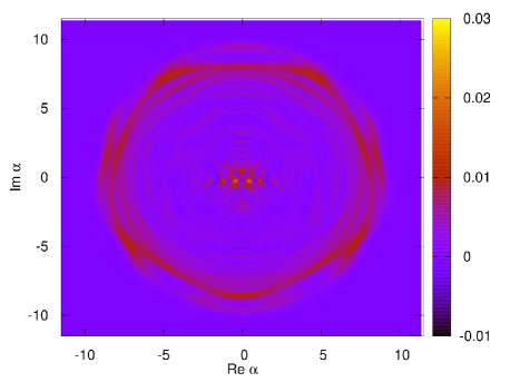
The broadening of the photon number distribution have effects in the phase space as well. Fig. 6 shows the Wigner function corresponding to the 15th HH mode in the long time limit. As we can see, this is not a localized wave packet, rather has a circular symmetry. This indicates the loss of phase information during the time evolution (resulting in quadrature expectation values close to zero, not shown in the figure). Although – according to Fig. 5 – corresponding to Fig. 6 is not a pure state, weak negative fringes around still indicate quantum mechanical interference and a nonclassical state.
That is, the time evolution of the system can be summarized as follows: At the initial stage the state of the system is close to a tensor product of coherent states. The magnitude of the labels for the HH mode coherent states are increasing linearly, while for the fundamental mode it is decreasing such that the ”weighted photon number” [E.q. (18)] is a constant of motion. When the photon number expectation value of the exciting mode becomes considerable lower than its initial value, this picture qualitatively changes, mode-mode entanglement builds up and all photon number distributions get broader. Also in the phase space, the Wigner functions become less localized. Or in terms of the eigenstates of the system: their initial superpositions lead to localized phase space distributions, but later on, as the phases of the eigenfunctions evolve, the distributions broaden. Since the problem is finite dimensional with discrete spectrum, the eigenstates can rephase leading to partial revivals.
V Summary
In the current paper we introduced a model for high-order harmonic generation in which both the exciting and the harmonic modes are treated as quantized fields. We adapted the Hamiltonian used for describing the process of parametric down-conversion to this problem by considering several HH modes. For an initial state which is the product of a coherent state (excitation) and vacuum states (HH modes), it was shown analytically that at the initial stage of the time evolution all fields are in coherent states. The parameters of these coherent states were explicitly given and verified by numerical calculations. For longer times, numerical results indicated a deviation from this behavior. The photon number distributions get broader, and – as it was shown by Wigner functions – localization in the phase space becomes less pronounced.
Acknowledgments
Partial support by the ELI-ALPS project is acknowledged. The ELI-ALPS project (GINOP-2.3.6-15-2015-00001) is supported by the European Union and co-financed by the European Regional Development Fund.
Á. G. acknowledges support from the project no. TKP2021-NVA-04 of the Ministry of Innovation and Technology of Hungary.
The work of B.G. Pusztai was supported by project TKP2021-NVA-09. Project no. TKP2021-NVA-09 has been implemented with the support provided by the Ministry of Innovation and Technology of Hungary from the National Research, Development and Innovation Fund, financed under the TKP2021-NVA funding scheme.
We thank Zsolt Divéki for the experimental data corresponding to Fig. 7.
*
.1 On the photon number statistics
In this appendix we shall study the time evolution of the photon number statistics for each mode. From this perspective it is crucial that the weighted photon number operator (18) and the interaction term (22) commute, and so the evolution operator associated with the Hamiltonian (1) factorizes as
| (26) |
To proceed further, let denote the parity operator of the HH mode . Upon introducing their product,
| (27) |
a moment of reflection reveals that
| (28) |
from where we obtain at once that
| (29) |
Turning to the photon number operators, clearly
| (30) |
Consequently, the relationship (29) entails that for all non-negative integer we have
| (31) |
and an analogous formula holds for each HH mode, too, simply by replacing letter with .
Now, our investigation hinges on the fact that the initial state (2) is compatible with in the sense that
| (32) |
Therefore, by exploiting (31), along the time evolution of for the th moment of the photon number statistics in the fundamental mode we get
| (33) | ||||
That is, the upshot of our symmetry argument is that each moment of the photon numbers statistics in the fundamental mode is an even function of time . Of course, the same argument applies to the HH modes as well. Giving a glance at (25), it readily follows that the time dependence of the Mandel parameter is also even. In particular, around , the power series expansions of the moments and the Mandel parameters contain only terms of even degree.
Keeping in mind the above observations, in the rest of the appendix we examine the short time behavior of the Mandel parameter for each mode. We perform the calculations in the Heisenberg picture, but for simplicity we omit the usual subscript from the time dependent operators. With this proviso, from (1) it is plain that the time evolution of the annihilation operators is governed by the following system of differential equations:
| (34) | |||
| (35) |
Note that, in terms of the auxiliary operators
| (36) |
the dynamics takes the somewhat simpler form
| (37) | |||
| (38) |
Furthermore, for the first two moments of the photon number statistics in the fundamental mode we can write
| (39) | |||
| (40) |
Of course, analogous formulae hold for the HH modes as well.
Since the system displayed in (37) and (38) is highly non-linear, we do not expect that its solution is expressible in closed form. Nevertheless, in order to capture the short time behavior of the photon number statistics, it is enough to work out the first few coefficients of the power series
| (41) |
Starting with the study of the fundamental mode, elementary calculations lead to the formulae
| (42) |
whereas for the second order coefficient we obtain
| (43) | ||||
Note that on the right hand sides of the above equations the operators and refer to the annihilation operators in the Schrödinger picture. Since for their action on the initial state (2) we have
| (44) |
for the time evolution of the expectation value (39) of the photon numbers in the fundamental mode we arrive at
| (45) |
Furthermore, utilizing (40), for the second moment we find
| (46) | ||||
Now, by plugging the above formulae into (25), for the Mandel parameter in the fundamental mode we end up with
| (47) |
We complete this appendix by examining the photon number statistics in the HH modes, too. It turns out that, contrary to the fundamental mode, the quadratic approximation in the power series (41) is not sufficient to derive the leading order behavior of the Mandel parameter. Nevertheless, by going one stage up, for the HH mode the cubic approximation of the power series leads to the estimation
| (48) |
However, the full control over the leading order behavior of does require even the fourth order terms in (41), thus the calculations are feasible only in the simplest special case of the second harmonic generation. Indeed, under the assumption that there is only a single HH mode characterized by , one can show that
| (49) |
.2 Modeling experimental results
Finally, let us consider a specific experimental example. Fig. 7 shows a part of the spectrum of argon gas that was excited by a pulse with 17.2 mJ energy at nm (duration: 28.1 fs intensity fwhm) using the SYLOS system of the ELI-ALPS [45]. The heights of the HH peaks are clearly not equal in this case, but we can choose appropriate parameters and to reproduce these peaks. Clearly, the parameter given by Eq. (13) cannot be constant in this case. Instead (according to the calculation in Sec. III) we choose e.g.:
| (50) |
where the numerical factors are the relative heights of the corresponding peaks in Fig. 7 (as compared to the 21st one.) Focusing on and 23 (), we performed numerical calculations with We used Eq. (50), and – as before – we considered two harmonic modes at a time, i.e., the pairs (21,19) and (21,23) were investigated. In both cases we found that the behavior of and () is quadratic in (c.f. Fig 1), and their ratio is close to at the beginning of the time evolution. More precisely, e.g., at the time instant when the photon number expectation value of the exciting mode dropped to 90% of its initial value, the relative difference between and was below 10%.
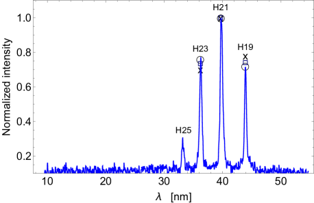
These calculations mean a direct connection between our model and experimental results, and demonstrate the flexibility of the approach introduced earlier in this paper.
References
- McPherson et al. [1987] A. McPherson, G. Gibson, H. Jara, U. Johann, T. S. Luk, I. A. McIntyre, K. Boyer, and C. K. Rhodes, Studies of multiphoton production of vacuum-ultraviolet radiation in the rare gases, J. Opt. Soc. Am. B 4, 595 (1987).
- Ferray et al. [1988] M. Ferray, A. L’Huillier, X. F. Li, L. A. Lompre, G. Mainfray, and C. Manus, Multiple-harmonic conversion of 1064 nm radiation in rare gases, J. Phys. B: At. Mol. Phys. 21, L31 (1988).
- Farkas and Tóth [1992] G. Farkas and C. Tóth, Proposal for attosecond light pulse generation using laser induced multiple-harmonic conversion processes in rare gases, Phys. Lett. A 168, 447 (1992).
- Quéré et al. [2006] F. Quéré, C. Thaury, P. Monot, S. Dobosz, P. Martin, J.-P. Geindre, and P. Audebert, Coherent wake emission of high-order harmonics from overdense plasmas, Phys. Rev. Lett. 96, 125004 (2006).
- Vincenti et al. [2014] H. Vincenti, S. Monchocé, S. Kahaly, G. Bonnaud, P. Martin, and F. Quéré, Optical properties of relativistic plasma mirrors, Nat. Comm. 5, 3403 (2014).
- Ghimire et al. [2011] S. Ghimire, A. D. DiChiara, E. Sistrunk, P. Agostini, L. F. DiMauro, and D. A. Reis, Observation of high-order harmonic generation in a bulk crystal, Nat. Phys. 7, 138 (2011).
- Ghimire and Reis [2019] S. Ghimire and D. A. Reis, High-harmonic generation from solids, Nat. Phys. 15, 10 (2019).
- Corkum [1993] P. B. Corkum, Plasma perspective on strong field multiphoton ionization, Phys. Rev. Lett. 71, 1994 (1993).
- Lewenstein et al. [1994] M. Lewenstein, P. Balcou, M. Y. Ivanov, A. L’Huillier, and P. B. Corkum, Theory of high-harmonic generation by low-frequency laser fields, Phys. Rev. A 49, 2117 (1994).
- Tsatrafyllis et al. [2017] N. Tsatrafyllis, I. K. Kominis, I. A. Gonoskov, and P. Tzallas, High-order harmonics measured by the photon statistics of the infrared driving-field exiting the atomic medium, Nat. Comm. 8 (2017).
- Tsatrafyllis et al. [2019] N. Tsatrafyllis, S. Kühn, M. Dumergue, P. Földi, S. Kahaly, E. Cormier, I. Gonoskov, B. Kiss, K. Varjú, S. Varró, and P. Tzallas, Quantum optical signatures in a strong laser pulse after interaction with semiconductors, Phys. Rev. Lett. 122, 193602 (2019).
- Bergou and Varró [1981a] J. Bergou and S. Varró, Nonlinear scattering processes in the presence of a quantised radiation field. II. Relativistic treatment, J. Phys. A: Math. Gen. 14, 2281 (1981a).
- Bergou and Varró [1981b] J. Bergou and S. Varró, Nonlinear scattering processes in the presence of a quantised radiation field. I. Non-relativistic treatment, J. Phys. A: Math. Gen. 14, 1469 (1981b).
- Gao et al. [1998] J. Gao, F. Shen, and J. G. Eden, Quantum electrodynamic treatment of harmonic generation in intense optical fields, Phys. Rev. Lett. 81, 1833 (1998).
- Chen et al. [2000] J. Chen, S. G. Chen, and J. Liu, Comment on “quantum electrodynamic treatment of harmonic generation in intense optical fields”, Phys. Rev. Lett. 84, 4252 (2000).
- Gonoskov et al. [2016] I. A. Gonoskov, N. Tsatrafyllis, I. K. Kominis, and P. Tzallas, Quantum optical signatures in strong-field laser physics: Infrared photon counting in high-order-harmonic generation, Sci. Rep. 6, 32821 (2016).
- Gombkötő et al. [2016] A. Gombkötő, A. Czirják, S. Varró, and P. Földi, Quantum-optical model for the dynamics of high-order-harmonic generation, Phys. Rev. A 94, 013853 (2016).
- Gombkötő et al. [2021] A. Gombkötő, P. Földi, and S. Varró, A quantum optical description of photon statistics and cross-correlations in high harmonic generation, Phys. Rev. A 104, 033703 (2021).
- Földi et al. [2021] P. Földi, I. Magashegyi, A. Gombkötő, and S. Varró, Describing high-order harmonic generation using quantum optical models, Photonics 8 (2021).
- Ákos Gombkötő [2023] Ákos Gombkötő, Squeezing properties of degenerate high-order hyper-raman lines emitted by a two-level system, Acta Physica Polonica Series a 143 (2023).
- Gombkötő et al. [2020] A. Gombkötő, S. Varró, P. Mati, and P. Földi, High-order harmonic generation as induced by a quantized field: Phase-space picture, Phys. Rev. A 101, 013418 (2020).
- Gorlach et al. [2020] A. Gorlach, O. Neufeld, N. Rivera, O. Cohen, and I. Kaminer, The quantum-optical nature of high harmonic generation, Nat. Comm. 11, 4598 (2020).
- Gorlach et al. [2023] A. Gorlach, M. E. Tzur, M. Birk, M. Krüger, N. Rivera, O. Cohen, and I. Kaminer, High-harmonic generation driven by quantum light, Nat. Phys. 10.1038/s41567-023-02127-y (2023).
- Stammer et al. [2023] P. Stammer, J. Rivera-Dean, A. Maxwell, T. Lamprou, A. Ordóñez, M. F. Ciappina, P. Tzallas, and M. Lewenstein, Quantum electrodynamics of intense laser-matter interactions: A tool for quantum state engineering, PRX Quantum 4, 010201 (2023).
- Walls and Tindle [1975] D. F. Walls and C. T. Tindle, Nonlinear quantum effects in second-harmonic generation, Lettere al Nuovo Cimento 2, 915 (1975).
- Kwiat et al. [1995] P. G. Kwiat, K. Mattle, H. Weinfurter, A. Zeilinger, A. V. Sergienko, and Y. Shih, New high-intensity source of polarization-entangled photon pairs, Phys. Rev. Lett. 75, 4337 (1995).
- Hochrainer et al. [2022] A. Hochrainer, M. Lahiri, M. Erhard, M. Krenn, and A. Zeilinger, Quantum indistinguishability by path identity and with undetected photons, Rev. Mod. Phys. 94, 025007 (2022).
- Walls and Milburn [1994] D. F. Walls and G. J. Milburn, Quantum Optics (Springer-Verlag, Berlin, 1994).
- Hillery et al. [1994] M. Hillery, D. Yu, and J. Bergou, Effect of the pump state on the behavior of the degenerate parametric amplifier, Phys. Rev. A 49, 1288 (1994).
- Louisell et al. [1961] W. H. Louisell, A. Yariv, and A. E. Siegman, Quantum fluctuations and noise in parametric processes. I, Phys. Rev. 124, 1646 (1961).
- Gordon et al. [1963] J. P. Gordon, W. H. Louisell, and L. R. Walker, Quantum fluctuations and noise in parametric processes. II, Phys. Rev. 129, 481 (1963).
- Hentschel et al. [2001] M. Hentschel, R. Kienberger, C. Spielmann, G. Reider, N. Milosevic, T. Brabec, P. Corkum, U. Heinzmann, M. Drescher, and F. Krausz, Attosecond metrology, Nature 414, 509 (2001).
- Paul et al. [2001] P. M. Paul, E. S. Toma, P. Breger, G. Mullot, F. Augé, P. Balcou, H. G. Muller, and P. Agostini, Observation of a train of attosecond pulses from high harmonic generation, Science 292, 1689 (2001).
- Hillery [1990] M. Hillery, Photon number divergence in the quantum theory of n-photon down conversion, Phys. Rev. A 42, 498 (1990).
- Schleich [2001] W. P. Schleich, Quantum Optics in Phase Space (Wiley-VCH, Berlin, 2001).
- Benedict and Czirják [1995] M. G. Benedict and A. Czirják, Generalized parity and quasi-probability density functions, J. Phys. A: Math. Gen. 28, 4599 (1995).
- Czirják and Benedict [1996] A. Czirják and M. G. Benedict, Joint Wigner function for atom - field interactions, Quantum and Semiclassical Optics: Journal of the European Optical Society Part B 8, 975 (1996).
- Mollow and Glauber [1967a] B. R. Mollow and R. J. Glauber, Quantum theory of parametric amplification. I, Phys. Rev. 160, 1076 (1967a).
- Mollow and Glauber [1967b] B. R. Mollow and R. J. Glauber, Quantum theory of parametric amplification. II, Phys. Rev. 160, 1097 (1967b).
- Drobný and Jex [1992] G. Drobný and I. Jex, Collapses and revivals in the energy exchange in the process of k-photon down-conversion with quantized pump, Phys. Rev. A 45, 1816 (1992).
- Bhattacharya et al. [2023] U. Bhattacharya, T. Lamprou, A. S. Maxwell, A. Ordonez, E. Pisanty, J. Rivera-Dean, P. Stammer, M. F. Ciappina, M. Lewenstein, and P. Tzallas, Strong-laser-field physics, non-classical light states and quantum information science, Reports on Progress in Physics 86 (2023).
- Czirjak et al. [2013] A. Czirjak, S. Majorosi, J. Kovacs, and M. G. Benedict, Emergence of oscillations in quantum entanglement during rescattering, Physica Scripta T153 (2013).
- Majorosi et al. [2017] S. Majorosi, M. G. Benedict, and A. Czirjak, Quantum entanglement in strong-field ionization, Phys. Rev. A 96 (2017).
- Maxwell et al. [2022] A. S. Maxwell, L. B. Madsen, and M. Lewenstein, Entanglement of orbital angular momentum in non-sequential double ionization, Nat. Comm. 13 (2022).
- Appi et al. [2023] E. Appi, R. Weissenbilder, B. Nagyillés, Z. Diveki, J. Peschel, B. Farkas, M. Plach, F. Vismarra, V. Poulain, N. Weber, C. L. Arnold, K. Varjú, S. Kahaly, P. Eng-Johnsson, and A. L’Huillier, Two phase-matching regimes in high-order harmonic generation, Opt. Express 31, 31687 (2023).