Abstract

Recommendation systems (RS) for items (e.g., movies, books) and ads are widely used to tailor content to users on various internet platforms. Traditionally, recommendation models are trained on a central server. However, due to rising concerns for data privacy and regulations like the GDPR, federated learning is an increasingly popular paradigm in which data never leaves the client device. Applying federated learning to recommendation models is non-trivial due to large embedding tables, which often exceed the memory constraints of most user devices. To include data from all devices in federated learning, we must enable collective training of embedding tables on devices with heterogeneous memory capacities. Current solutions to heterogeneous federated learning can only accommodate a small range of capacities and thus limit the number of devices that can participate in training. We present Federated Averaging in Random subspaces (FAIR), which allows arbitrary compression of embedding tables based on device capacity and ensures the participation of all devices in training. FAIR uses what we call consistent and collapsible subspaces defined by hashing-based random projections to jointly train large embedding tables while using varying amounts of compression on user devices. We evaluate FAIR on Neural Collaborative Filtering tasks with multiple datasets and verify that FAIR can gather and share information from a wide range of devices with varying capacities, allowing for seamless collaboration. We prove the convergence of FAIR in the homogeneous setting with non-i.i.d data distribution. Our code is open source at https://github.com/apd10/FLCF

1 Introduction

Recommendation systems (RS) form the backbone of a good user experience on various platforms, such as e-commerce websites, social media, streaming services, and more. RS solves the issue of information overload by helping users discover the information most pertinent to them. To provide personalized suggestions, RS collects user features such as gender, age, geographical information, etc., and past user activity on the platform. User feedback can be categorized as either explicit feedback, such as ratings, or implicit feedback, such as views, clicks, or time spent on an item.

Traditionally, the user feature and interaction data is collected on a server, and RS models are trained centrally. However, several studies Calandrino et al. (2011); Lam et al. (2006); McSherry & Mironov (2009) have exposed the privacy risk associated with the centralized collection of data. Even seemingly benign interaction data, such as movie ratings, can be used to deduce personal details such as age, gender, and political affiliations Weinsberg et al. (2012); Aonghusa & Leith (2016); Narayanan & Shmatikov (2008). Owing to such risks, regularization of data usage and protection is increasingly necessary. One such legislation in the European Union is the General Data Protection Regulation (GDPR), which regulates data usage conditions by platforms. Federated learning, a distributed machine learning paradigm, ensures that user data never leaves its respective device—an apt solution for data privacy.

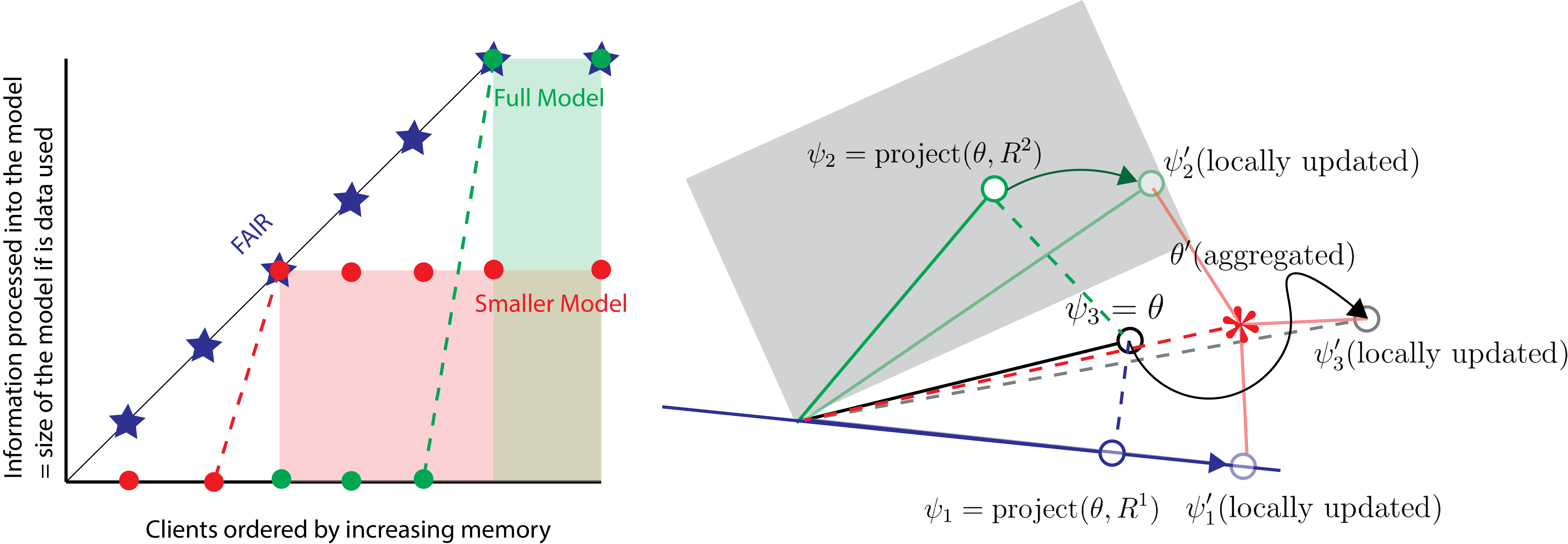
Figure 1: [Left] Consider the information contributed by a device as the model-size trained with local data. Illustration shows 2/7 devices can host full model. Thus, under traditional settings, we can only run federated learning with those two devices. To include more devices we need to reduce the model size. With a smaller model we can include, perhaps, 5/7 devices but the information quality is lower for all (red plot). FAIR provides smooth trade-off where each device can host a different sized model and contribute information based on its capacity. [Right] Illustration of FAIR. Let the parameter be in $R^{3}$, There are three devices which can store parameter sizes of 1 (blue), 2 (green) and 3 (black) respectively. In each round, FAIR projects the $\theta$ vector (dark black circle) to random sub-spaces of dimensions 1 and 2. Devices with capacity of 3 can directly use $\theta$. Models are optimized inside the sub-spaces locally, and then aggregated back at the server (red) in $R^{3}$.

RS models, such as collaborative filtering (CF) models like MF Koren et al. (2009), NeuMF He & Chua (2017), etc., and ad recommendation click-through models, such as DLRM Naumov et al. (2019), Deep Factorization Model Guo et al. (2017), etc. have embedding tables for items and other categorical features. These embeddings are typically very large due to large product catalogs and other categorical data. For instance, Pinterest has billions of pins for recommendation Pal et al. (2020), and Amazon offers 100s of millions of products—leading to multiple gigabyte-sized embedding tables. To train a federated learning-based RS model, the model must necessarily fit onto client devices. Given the scale of these embedding tables, many client devices (such as mobile phones or low-memory laptops) simply cannot store the full model.

Thus, the problem of client device heterogeneity (with respect to memory capacity) is especially pronounced in the context of RS models. Devices such as desktops and laptops can potentially hold full RS embedding tables, whereas devices such as mobile phones cannot. Two naive solutions to this issue are: (A) to discard data from devices that cannot fit the model (data loss) or (B) to learn a smaller model to incorporate all devices (model loss). There is a natural trade-off where model size determines the devices that can participate in federated learning. This trade-off is shown in Figure 1. FAIR can customize the quality of information obtained from a device based on its capacity while building a full-sized model on the server. Thus, with FAIR, all devices with arbitrarily small memory capacity can still participate in federated learning.

The general recipe of FAIR is shown in Figure 2, which includes communicating with a device that cannot host the entire model. FAIR uses hashing-based random projections in combination with recent advances in efficient parameter-sharing kernels Desai et al. (2022a; b) to reduce the memory footprint of the model and train on-device while only realizing a reduced memory cost. As illustrated in the toy example in Figure 1, each device is associated with a random projection matrix (and hence a subspace). The parameters of the model are only stored in the subspace basis, thus reducing the model’s memory footprint. Additionally, the parameters are optimized within this subspace and thus never fully realized in memory. Naively selecting random projections is detrimental to the collaborative training of the model. FAIR proposes the use of consistent and collapsible subspaces which have provable convergence guarantees. A complete definition of consistent and collapsible subspaces is included in Section 4.3. More details on intelligently building random projection matrices and model training without realizing the full model size are provided in Section 4.

In our experimental results, we show that FAIR provides better quality models over both alternatives of data-loss (excluding devices) and model-loss (using smaller models). Additionally, it outperforms heterogeneous federated learning baselines such as FEDHM Yao et al. (2021) and HETEROFL Diao et al. (2020) on embedding tables. Furthermore, it enables us to include devices having smaller capacities that baseline methods cannot support. We also show that FAIR is a general strategy that can be extended to other model components, such as convolutions and MLPs.

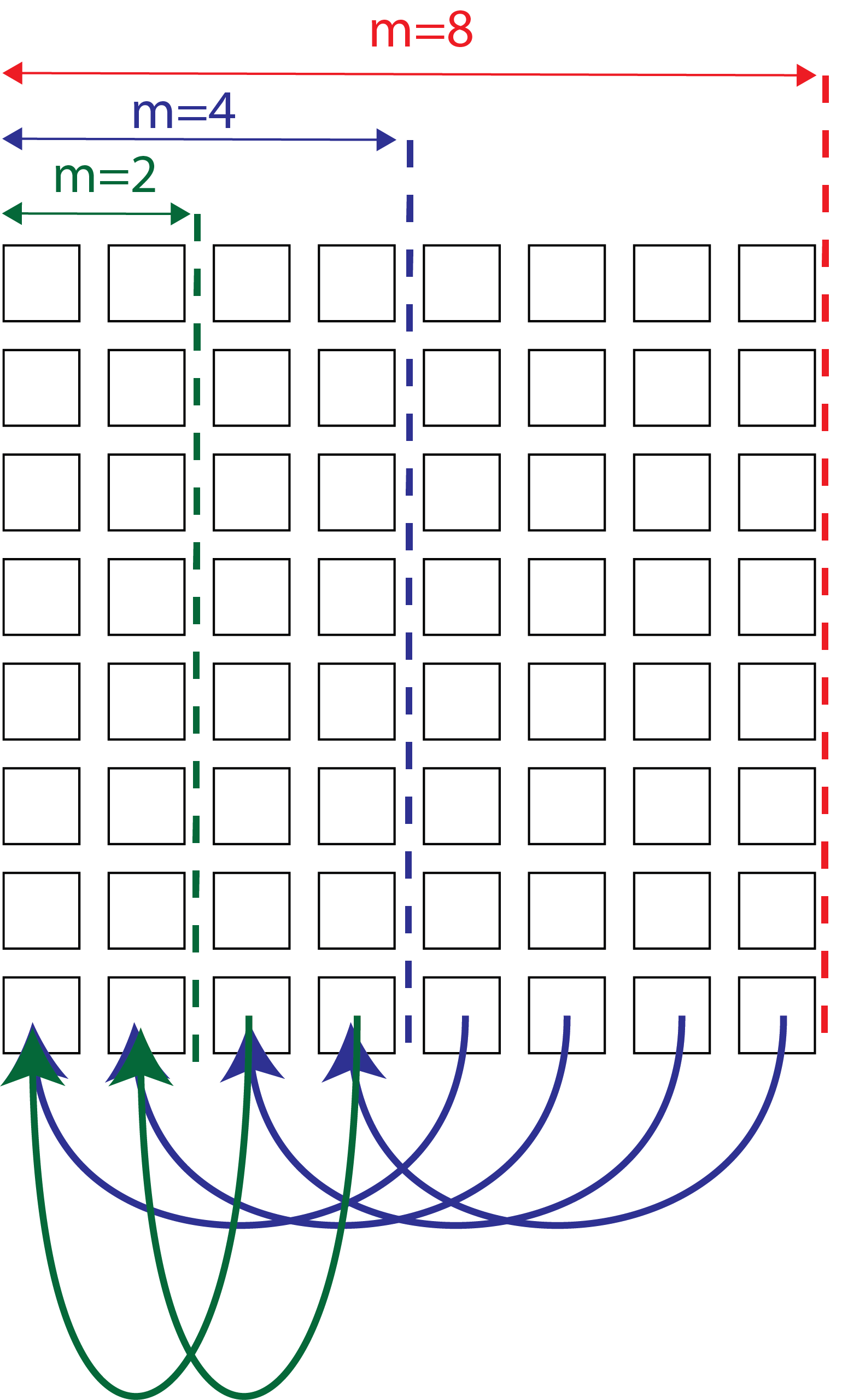
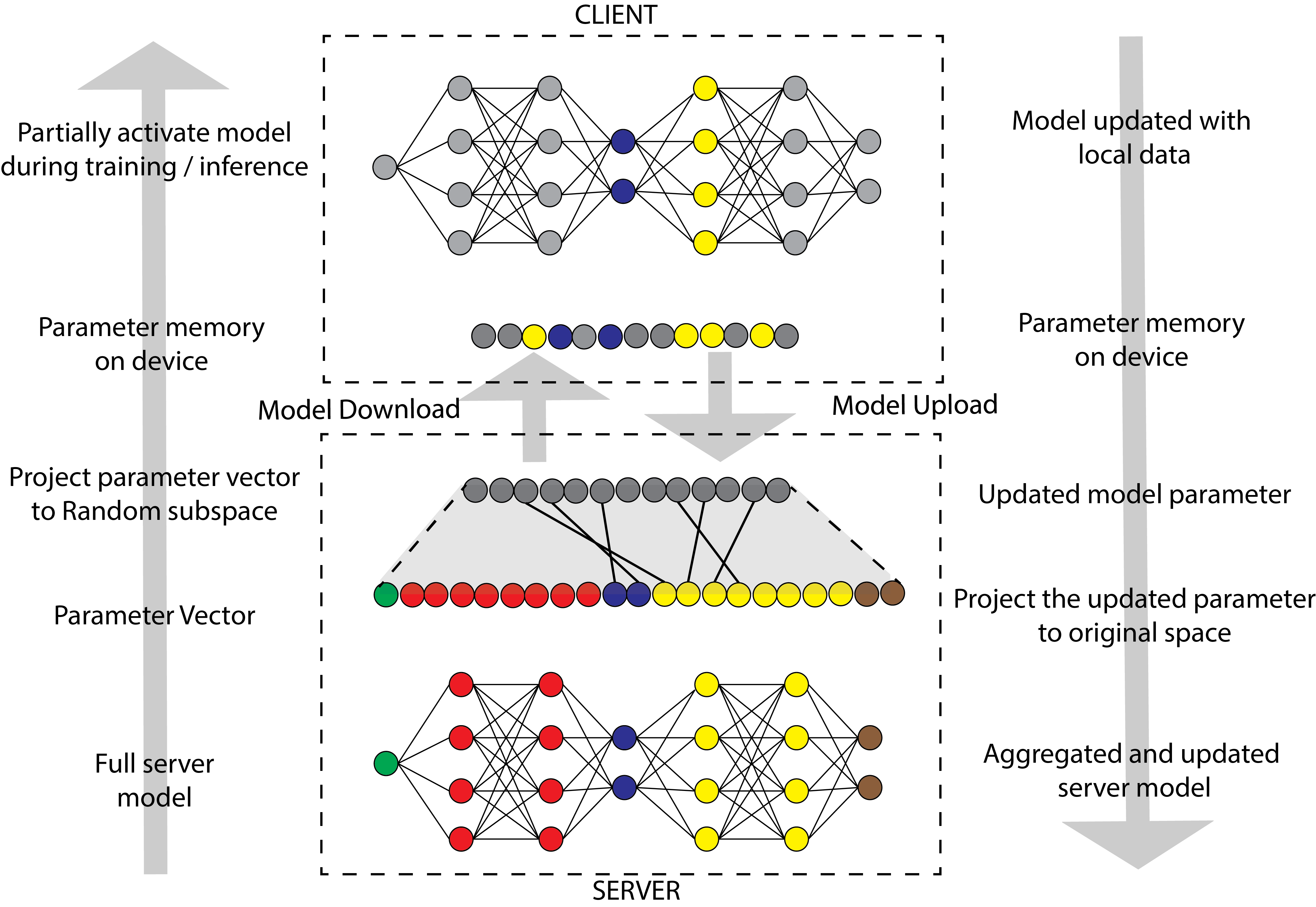
Figure 2: [Left] Illustration of matrix clip-and-add to create a set of consistent and collapsible subspaces. The original $n\times m$ matrix is generated by the hash function $h$. Then depending on the target size $m_{i}$ for a device $i$, the matrix is cut into $m/m_{i}$ pieces and all the pieces are added to each other. [Right] A round associated with FAIR: The server projects its parameter vector $\theta$ into a smaller vector $\psi$ and sends this vector to the client. The client stores the smaller vector $\psi$ and trains it locally using memory efficient parameter sharing based kernels. The updated $\psi$ is sent back to the server which is expanded into $\theta$ and aggregated with parameters received from other devices.

Limitations: FAIR can be applied to embedding tables as well as other generic model components such as convolutions, MLPs, etc. However, one concern when applying FAIR to model components other than embedding tables is that FAIR does not reduce the computational workload of the compressed model. Thus, FAIR is most suitable for memory-heavy components such as embedding tables, which only require table lookups or indexing—making it a perfect solution to embedding-heavy recommendation models. We would, however, like to stress that FAIR can provide arbitrarily small memory footprints, which cannot be achieved by other methods, making it possible to include all client devices, which is impossible with existing approaches to heterogeneous federated learning.

2 Related Work

Federated learning is a distributed training approach in which model training occurs on user devices, preserving data privacy. A central server coordinates the process, sending initial model parameters to user devices, which subsequently train the model on local data and upload updated parameters to the server. Communication occurs in a staggered manner to reduce network overhead. Model updates from devices are aggregated using algorithms like FEDAVG McMahan et al. (2017) or FEDProx Li et al. (2020a), which average the model parameters from each participating device.

Research around federated learning in the context of recommendation systems has gained momentum in the past couple of years Lin et al. (2020); Muhammad et al. (2020); Tan et al. (2020); Liang et al. (2021); Shi et al. (2021). Some specific aspects of federated recommendation systems have been widely studied, such as privacy in Li et al. (2020b); Gao et al. (2020); Wang et al. (2020); Chen et al. (2020); Qi et al. (2020); Chen et al. (2022) and fairness Maeng et al. (2022); Liu et al. (2022). However, the memory issues associated with recommendation models— primarily due to the enormous embedding tables part of most recommendation models—have not been investigated. This paper considers arguably the simplest setting of CF recommendation models to discuss the issue of large embeddings in federated learning.

Federated learning for CF models has been previously studied in the literature. Analysis has been made of existing algorithms using alternating least squares and stochastic gradient updates in the context of federated CF models Ammad-Ud-Din et al. (2019). Differential privacy concerns have also been investigated within the context of communicated data in federated CF Minto et al. (2021); Jiang et al. (2022). To the best of our knowledge, we are the first to examine the issue of heterogeneous memory capacities of client devices, which need to participate in federated learning of a CF model and provide an efficient solution that can effectively collaborate information across heterogeneous models on different devices.

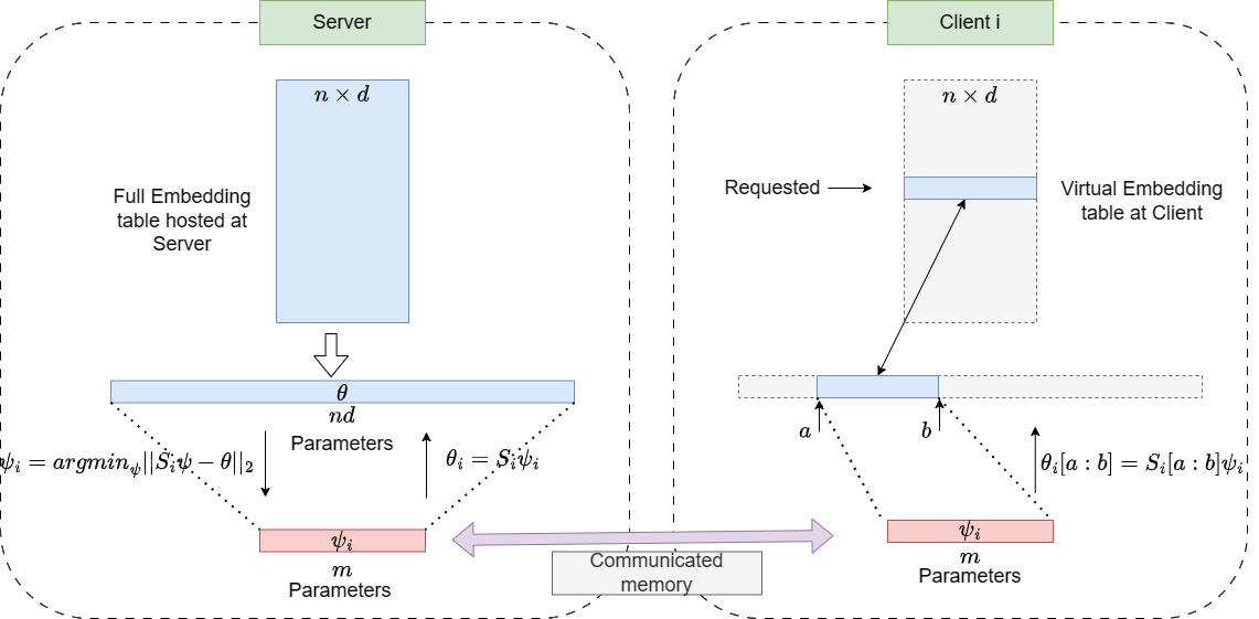
Figure 3: Illustration of how embedding tables are distributed to limited capacity devices, trained and updates are communicated taking one client as an example. In the figure, the entire embedding table of size $n\times d$ is hosted in server and has $nd$ sized parameter vector. The client device is associated with a (sparse) projection matrix $S$ generated with hash function. The server first projects the parameter vector to smaller column subspace of $S$ giving compressed vector $\psi$. The $\psi$ parameters are transmitted to device and trained on device. While training and inferring concrete parts of virtual embedding table (not realized) are recovered from the $\psi$ as required. While uploading, $\psi$ is uploaded to server and projected to server basis using $S\psi$. The server collects all such vectors from different clients. The $\theta_{i}$s thus received will then be used to update the server model $\theta$. In this paper we use FEDAVG, but we can potentially use any algorithm once all $\theta_{i}$s are collected

Recently, a few approaches have been explored for the problem of heterogeneity in storage and communication capacity in federated learning. The basic idea is to send smaller versions of models to clients with lower capacities. Both low-rank factorization and slices of weight matrices have been used to create smaller versions of models Yao et al. (2021); Diao et al. (2020). However, in both approaches, there is a fundamental limit to the amount of memory reduction that can be achieved. The issue is especially burdensome when applying compression techniques for embedding tables (say $n\times d$), which, at times, are orders of magnitude larger than what user devices can store. While these methods can—at best—accommodate clients that need less than $d\times$ compression, FAIR can accommodate any client with an arbitrarily small memory capacity.

Table 1: Lowest capacity supported by various heterogenous FL methods

($E:n\times d$)	FEDHM	HETEROFL	FAIR
Max Compression	$<d\times$	$d\times$	Arbitrary

3 Background : Parameter sharing based compression

Recently, randomized parameter sharing has shown promising results for model compression with HashedNetChen et al. (2015), ROBE (Desai et al., 2022a) and ROAST (Desai et al., 2023). FAIR is also based on parameter sharing, and thus, we briefly explain how parameter sharing has been used for model compression in literature.

The general recipe of parameter sharing-based model compression is as follows. Consider a given model with a total number of parameters $n$. Under parameter sharing-based compression, there is a parameter repository $\mathcal{M}$ such that $|\mathcal{M}|<n$. The model weights are not explicitly stored in memory but are “virtual". The only concrete parameter memory that is stored and trained is $\mathcal{M}$. The computational graph of the model is the same, and whenever we want to access the model weight, say a parameter $w$ of some layer inside the model, we use a hash function, say $h$, to locate the weight inside the repository of parameters. Thus, the value of $w$ is

$$w=\mathcal{M}[h(id(w))]$$ (1)

Optionally, another hash function $g$ with range $\{\pm 1\}$ is multiplied with the retrieved value to obtain the final weight value. i.e. $w=g(id(w))\mathcal{M}[h(id)]$.

To the best of our knowledge, HashedNet was the first to propose parameter sharing-based compression. They used element-wise hash functions, which independently map each weight into the repository. One of the issues in this mapping is the cache-inefficiency as in order to retrieve, say, an embedding of size $d$, $d$ separate potentially faraway locations need to be accessed. The issue of cache-inefficiency is fixed in ROBE for embedding tables and ROAST for matrix multiplication operation.

4 FAIR: Federated Averaging in Random Subspaces

As mentioned earlier, FAIR is best suited for models with large embedding tables, and thus, the focus of this paper is federated CF. However, the design of FAIR is general and can be applied to other model components. In this section, we describe FAIR in the most general manner. We refer to the parameter vector $\theta$ (a flat vector of all model parameters being optimized), which may only include embedding table parameters in the context of CF models or other model components if needed.

The key idea in FAIR is that each device stores a model representation $\psi\in R^{k}$, which can be of smaller dimension than $\theta\in R^{n}$. The two representations are linked via a subspace defined by column space of $S\in R^{n\times k}$, also called the projection matrix. Simply put, in order to get $\psi\in R^{k}$, we project $\theta$ on the column subspace of $S$, and $\psi$ is the projected vector in the new basis of column-space ($S$). To recover the model in the server basis, we can just compute $S\psi$. When running the model on the client, we always maintain $\psi$ in memory but recover the parts of the model, say $\theta[a:b]$ for some $a,b$ in the original space using $S[[a:b],:]\psi$ as needed. This is illustrated in Figure 2 (right) and Figure 3. We will discuss the details of these operations and how to choose these subspaces below.

Notation (federated learning):

We will use the following notation throughout the paper. The total number of devices is $N$, and in each round of federated learning, we will be sampling $K$ ($K\leq N$) devices. The training is conducted for $T$ rounds, each of which consists of $E$ steps of SGD. The optimization function associated with each device and its data is denoted as $F_{i}(\theta,\mathcal{D}_{i})$ where $\theta$ is the parameter vector and $\mathcal{D}_{i}$ is the data associated with device $i$.

Notation (FAIR):

Under FAIR, we denote the server parameter-vector as $\theta\in R^{n}$. Each device $i$ has a capacity $0<\alpha_{i}\leq 1$ and stores a parameter vector $\psi_{i}\in R^{m_{i}}$ where $m_{i}\leq\alpha_{i}n$. Each device is associated with a subspace of dimension $m_{i}$, which is denoted by the column space of an orthogonal (column) matrix $S_{i}:n\times m_{i}$. The optimization functions of device $i$ are denoted as $F^{\prime}_{i}(\psi_{i},\mathcal{D}_{i})=F_{i}(S_{i}\psi_{i},\mathcal{D}_{i})$. We denote $\theta_{i}=S_{i}\psi_{i}$. $\theta_{i}$ and $\psi_{i}$ are the same vectors in different bases. We call the basis of $\theta$ the server-basis and that of $\psi$ the device-basis.

4.1 Hashing-based random projections and associated subspaces

In this section, we elaborate on how computationally cheap hash functions can be used to create random projection matrices (and hence subspaces), which can be stored in $O(1)$ memory and applied in $O(n)$ time. We also define the reduction and recovery operations for transitioning between the server model and device models.

Consider a client with capacity $\alpha$. FAIR assigns a subspace to each client based on its capacity. The subspace is defined by a projection matrix, say $S\in R^{\hskip 1.0ptn\times m}$ where $m\leq\lfloor\alpha n\rfloor$ Using dense projections such as Gaussian are expensive, both in terms of the memory required to store the projection and to compute the projections of a given vector. Hence, we use hashing-based sparse projections. Examples of good projections for our purpose would include count-min-sketch (CMS) Cormode & Muthukrishnan (2005) count-sketch (CS) Charikar et al. (2002), ROBE Desai et al. (2022a), ROASTDesai et al. (2023) etc. We will discuss CMS for its simplicity in this section. However, the discussion can be trivially extended to other mappings. In our experiments, we use ROAST mapping. CMS mapping is a binary matrix $S_{cms}$, and is defined as follows:

$$S_{cms}[i,j]=1\iff h(i)=j$$ (2)

Note that each row of the matrix has exactly $1$ non-zero and the location is determined by hash function $h:\{0,\dots,n{-}1\}\rightarrow\{0,\dots,m-1\}$ where $h$ is drawn from the family of universal hash functions Carter & Wegman (1977) that require $O(1)$ memory and $O(1)$ computation. The matrix $S$ is never realized in memory. We only store $h$ to compute $S[i,j]$ on the fly as required using Equation 2.

Algorithm 1 FAIR: Heterogeneous Federated Averaging in Random Subspaces (Server)

Requires :

$N$ devices with data $\{\mathcal{D}_{i}\}_{i=1}^{N}$; capacity ratios $\{\alpha_{i}\}^{N}_{i=1}$; $0<\alpha_{i}\leq 1$; loss function $F(\theta,\mathcal{D})$; initial parameter vector at the server, $\theta$.

Initialize $\theta$

for round, $t\in[0,\dots,T-1]$ do

      9876543 $\theta^{\prime}\leftarrow 0$  Generate seed for hash function $h$  $C\leftarrow$ a random set of clients  Communicate seed to clients in $C$  $\forall i\in C,S_{i}\leftarrow$ the projection matrix corresponding to capacity $\alpha_{i}$ according to Equation 7  /* These matrices are not realized, hashing is performed on-the-fly */ $\psi_{i}\leftarrow$ projection$(S_{i},\theta)$ according to the Equation 4 operation  foreach client, $i\in C$, in parallel do

            13121110 Send $\psi_{i}$  $\psi_{i}^{\prime}\leftarrow$ wait for client update  $\theta_{i}^{\prime}\leftarrow S_{i}\psi_{i}^{\prime}$ projection according to Equation 5 operation  $\theta^{\prime}\leftarrow\theta^{\prime}+p_{i}\theta_{i}^{\prime}$ ;

              /* $p_{i}$ are the aggregation weights in fed-avg aggregation is atomic to avoid data race */

       end foreach

      14$\theta\leftarrow\theta^{\prime}$ 

end for

Algorithm 2 FAIR: Heterogeneous Federated Averaging in Random Subspaces (Client $i$)

Requires :

Data $\{\mathcal{D}_{i}\}$; capacity ratio $0<\alpha_{i}\leq 1$; loss function $F(\theta,\mathcal{D})$.

Receive seed for hash function $h$

Receive $\psi_{i}$

Optimize $F_{i}(\mathcal{D}_{i},\psi_{i})=F(\mathcal{D}_{i},S_{i}\psi_{i})$ for $E$ epochs on local data $\mathcal{D}_{i}$  /* Training done in a memory efficient manner using kernels from Desai et al. (2022a), Desai et al. (2022b) which use the 6 equation */

Send updated $\psi_{i}$ to server

Reduction (server model to client model):

Projecting $\theta$ onto the subspace defined by $S$ to obtain $\psi_{S}$, is equivalent to finding a solution to the equation:

$$\psi_{S}=\textrm{argmin}_{\psi_{S}}||S\psi_{S}-\theta||_{2}$$ (3)

Generally, this linear system of equations can be solved using normal equations or SGD. However, with a sparse $S$ such as those defined by CMS, we have a simple solution:

$$\psi_{S_{cms}}[j]=\frac{\sum_{i}\theta[i]\mathbf{I}(h(i){=}j)}{\sum_{i}\mathbf{I}(h(i){=}j)}=S_{cms}^{\top}\theta/S_{cms}^{\top}\mathbf{1}^{(n)}$$ (4)

This can be implemented by computing $S_{cms}^{\top}\theta$ and performing element wise division by the counts $S_{cms}^{\top}\mathbf{1}^{(n)}$ where $\mathbf{1}^{(n)}$ is the $n$-dimensional column vector of $1$s. Due to the sparse $S_{cms}$, this is a $O(n)$ time operation.

Recovery (client model to server model):

The vector $\psi_{S}\in R^{\hskip 1.0ptm}$ is in the basis of $S$. In order to recover the vector in the original $R^{n}$ space, we compute:

$$\theta_{S}=S\psi_{S}$$ (5)

Note that $\theta_{S}$ is the vector in the column space of $S$, and $S$ is simply a change of basis matrix.

In typical federated learning settings, the server broadcasts $\theta$ at the beginning of each round, and clients return $\psi_{S}$ at the end of each round. The reduction operation is required when the server needs to send $\psi_{i}$, and the recovery operation is required when the server receives $\psi_{S}$ as shown in figure 2 (right). Alternatively the server can broadcast $\theta$ and the client can project it in a streaming fashion to obtain $\psi_{i}$. For the discussion, we assume the former setup.

4.2 Running model on the client without realizing full memory

As described above, $\psi_{S}$ is the model representation used on a client device. Under FAIR, the optimization function computation is still $F(S\psi,\mathcal{D})$. In other words, the computation has not changed. How can the model run on the device without incurring $|S\psi|=n$ memory? The idea is straightforward—the client only realizes parts of the full model that are necessary at the time of computation. For instance, in an embedding table lookup, we only need access to some particular embeddings in a batch. See illustration in Figure 3. To retrieve the embedding parameters located at, say $\theta[a:b]$, we can use:

$$\theta[a:b]=S[a:b,:]\psi_{S}$$ (6)

Recent advances in parameter-sharing methods provide efficient kernels based on partial recovery, such as those for embedding tables Desai et al. (2022a) and matrix multiplication Desai et al. (2022b).

4.3 Consistent and collapsible subspaces

The choice of subspaces is important for effective collaboration of information among devices. As an example, consider two randomly drawn $1$-dimensional subspaces in $R^{n}$. For a large $n$, with high probability, these subspaces are orthogonal. Thus, the information transferred from one subspace to another via projection is nil as any vector in one subspace, when projected onto another, will go to $\mathbf{0}$. Thus, we must choose a set of consistent and collapsible subspaces as defined below.

Definition 4.1 (Consistent and Collapsible Subspaces).

A given set of subspaces defined by columns of matrices $\{S_{i}\}_{i=1}^{N}$ where $S_{i}:n\times m_{i}$ matrix, is consistent if, for every pair $i,j$, if $m_{i}=m_{j}$ then column-space of $S_{i}$ is the same as the column-space of $S_{j}$. Also, if $m_{i}<m_{j}$, then $\textrm{column-space}(S_{i})\subset\textrm{column-space}(S_{j})$.

The compatibility between two subspaces for information sharing can be measured by the angles between the two subspaces. By considering subspaces contained inside one another, we maximize the compatibility of the subspaces. In FAIR, each unique subspace is identified by a single projection matrix $S$. Thus, a consistent and collapsible subspace associated with all devices, including the server, implies using the exact same basis for all devices that can host the full model. This also implies that if all participating devices can host full models, FAIR is identical to standard FEDAVG.

We now show how to construct these subspaces using lightweight hash functions when the parameter sizes on devices $\{m_{i}\}$ are powers of 2. Depending on the capacity $\alpha$, the parameter size, $m_{i}$, is taken to be the greatest power of $2$ smaller than $\alpha_{i}n$.

Constructing consistent and collapsible subspaces using hashing:

Let $m=\max(\{m_{i}\})$. We draw the hash function $h:\{0,\dots,n-1\}\rightarrow\{0,\dots,m-1\}$ from a family of cheap hash functions such as the universal family Carter & Wegman (1977). The set of subspaces is then defined as follows. Let each device have a subspace represented by an orthogonal matrix $S_{i}$. We define the binary $S_{i}:n\times m_{i}$ as follows:

$$S_{i}[a,b]=1\quad\textrm{iff}\quad h(a)\%m_{i}=b$$ (7)

Note that each row of $S_{i}$ only has one non-zero element. Thus, each column of $S_{i}$ is orthogonal to every other column. We can convert this matrix into an orthonormal matrix by normalizing each column to the unit norm.

Theorem 4.2.

The set of subspaces $\{S_{i}\}_{i=1}^{N}$ of dimensions $\{m_{i}\}_{i=1}^{N}$, where each $m_{i}$ is a power of 2, created using the hash function $h$ as per Equation 7, is a consistent and collapsible set of subspaces.

This computation is illustrated in Figure 2 (left). Essentially, we first create a matrix $S$, which is of dimension $n\times m$. Then, in order to create the matrix $S_{i}$ for subspace $i$, we cut the matrix in columns of width $m/m_{i}$ and add the pieces together. This also provides an intuition for why this set of subspaces is collapsible: given any two matrices $S_{i}$ and $S_{j}$, if $m_{i}<m_{j}$, then each column of $S_{i}$ is the sum of $m_{j}/m_{i}$ columns of $S_{j}$, and hence, column-space($S_{i}$) $\subset$ column-space($S_{j}$). We want to emphasize that these computations occur on the fly, and no matrix is actually realized.

4.4 FAIR Algorithm

The complete algorithm of FAIR is provided in Algorithm 1. At each round, the server projects the parameter vector $\theta$ onto the subspaces associated with each client sampled for that round using 4 operations and sends the parameter in the device-basis, $\{\psi_{i}\}$, to the clients. Client $i$ optimizes the function $F(S_{i}\psi_{i},\mathcal{D}_{i})$ using local data $\mathcal{D}_{i}$ with $\psi_{i}$ residing inside the subspace associated with $S_{i}$. Clients employ efficient parameter-sharing kernels using 6 equations, which ensure that the memory footprint of the model remains $|\psi|$. After $E$ steps, the client sends the updated $\psi_{i}$ back to the server, which is transformed into a server-basis using a 5 operation and aggregated with updated models from other clients using standard FEDAVG weighted aggregation.

5 Convergence of FAIR

Empirically, we can see that consistent subspaces are necessary for convergence, as shown in Figure 4. In this section, we prove the convergence of FAIR in homogeneous settings where models are compressed equally on all devices.

Recently, $O(\frac{1}{T})$ convergence of federated learning on non-iid data with full and partial participation of devices was proven Li et al. (2019) when the following conditions (paraphrased from Li et al. (2019)) are met: (1) $F_{1}$, … $F_{N}$ are L-smooth; (2) $F_{1}$, …. $F_{N}$ are $\mu$-strongly convex; (3) variance of stochastic gradients on all the devices is bounded. If $\zeta_{t}^{k}$ is the stochastic sample for device $k$ at round $t$, then $\mathbb{E}||\nabla F_{K}(\theta^{k}_{t},\zeta_{T}^{k})-\nabla F_{K}(\theta^{k}_{t},\mathcal{D}_{k})||^{2}\leq\sigma_{k}^{2}$; and (4) expected squared norm of the stochastic gradients is uniformly bounded, $\mathbb{E}(||\nabla F_{k}(\theta^{k}_{t},\zeta^{k}_{t}||^{2}\leq G^{2})$ for all devices and rounds. For the exact expression of convergence, we refer the reader to Li et al. (2019). The convergence of FAIR under homogeneous conditions with full participation (alt. partial participation) can be stated as the corollary of Theorem 1 (alt. Theorem 2, 3 in Li et al. (2019)). We first need two lemmas to complete the proof.

Lemma 5.1.

Under FAIR notation, if $F_{1},F_{2},\dots,F_{N}$ satisfy the assumptions 1-4 above, and $F^{\prime}_{1},F^{\prime}_{2},\dots,F^{\prime}_{N}$ are:

$$F^{\prime}_{i}(\psi)=F_{i}(\mathcal{S}\psi)\qquad\forall i\in\{1,\dots,N\}$$ (8)

If $\mathcal{S}$ is an orthonormal matrix, then $F^{\prime}_{1},F^{\prime}_{2},\dots,F^{\prime}_{N}$ also satisfy the assumptions 1-4 with the same constants $L,\mu,\sigma_{k},G$ for all $k\in\{1,\dots,N\}$.

Lemma 5.2.

Under FAIR notation and with a unique subspace matrix $S$ across all the devices, the server parameter-vector $\theta_{S}$ can always be represented as $\theta_{S}=S\psi$ for some $\psi$. And the parameter aggregation equation can be written as $\psi=\sum_{i=1}^{N}p_{i}\psi_{i}$ where $p_{i}$ are weights of aggregation as per standard $\mathrm{FEDAVG}$.

Proof of Lemma 5.1 is provided in the Appendix. With Lemmas 5.1 and 5.2, we can cast the entire federated learning with FAIR under homogeneous settings as federated learning with parameters in the subspace $S$ (even at the server). Thus, the convergence of FAIR can be stated as a corollary to Theorem 1, 2, 3 from Li et al. (2019). We only state the concise form of Theorem 1 here:

Corollary 5.3.

If the functions $F_{1},\dots,F_{N}$ satisfy assumptions 1-4, then under the homogeneous setting of FAIR (equal dimension of random subspace), the algorithm converges at a rate $O(\frac{1}{T})$.

6 Experiments

Table 2: [NDCG@20 (higher is better) on Goodreads-100, AmazonProduct-100]. FAIR-HET has superior quality over FAIR-HOM and FEDHM baselines across different capacity schemes. N/A implies that capacity scheme cannot be run. std-deviation ($<0.005$ for Goodreads-100 and $<0.009$ for AmazonProduct-100)

	Goodreads-100			AmazonProducts-100
Central Training	0.28			0.20
FEDAVG	0.278			0.178
Capacity	FAIR-HET	FAIR-HOM	FEDHM	FAIR-HET	FAIR-HOM	FEDHM
1x-2x	0.276	0.269	0.274	0.13	0.10	0.078
1x-4x	0.276	0.254	0.275	0.14	0.098	0.041
1x-8x	0.274	0.246	N/A	0.087	0.07	N/A
1x-16x	0.276	0.208	N/A	0.056	0.06	N/A

Table 3: NDCG for Goodreads-100 and AmazonProducts-100. Comparison of FAIR-HET with the situation where data from lower-capacity devices is not used (FULL-TRN). The columns define percentage of users that can host full models (1x capacity) and others are assumed to have 2x compression. The users are randomly chosen with seed 101. Thus the sets for each column can be non-overlapping.

	Goodreads-100				AmazonProducts-100
	1%	20%	30%	50%	1%	20%	30%	50%
FULL-TRN	0.037	0.247	0.238	0.261	0.003	0.006	0.05	0.09
FAIR-HET	0.271	0.258	0.27	0.258	0.107	0.109	0.110	0.121

Table 4: Explicit feedback rating prediction on Goodreads-100 (MSE lower is better). We stop training after 1000 rounds. The FEDHM method cannot cater to compression ratios of 32 or beyond for an embedding table of 32 dimension. N/A implies the scheme cannot be run.

Capacity	FAIR-HET	FAIR-HOM	FEDHM
8x-16x	0.6735	0.6891	0.7243
16x-32x	0.6716	0.6907	N/A
32x-64x	0.6726	0.6916	N/A
4x-8x-16x	0.6618	0.6891	0.7206
8x-16x-32x	0.6607	0.6907	N/A
16x-32x-64x	0.6618	0.6916	N/A

Table 5: Test accuracy results of different model capacity settings compared to (uncompressed) full FEDAVG MNIST and FEMNIST datasets. N/A implies the scheme cannot be run.

	MNIST			FEMNIST
FEDAVG	0.9841			0.7491
Capacity	FAIR-HET	FAIR-HOM	FEDHM	FAIR-HET	FAIR-HOM	FEDHM
2x-4x	0.9822	0.9829	0.9838	0.7842	0.7847	0.7804
2x-4x-8x	0.9823	0.9779	0.984	0.7691	0.779	0.7689
2x-4x-8x-16x-32x-64x	0.9636	0.962	0.9839	0.7409	0.7114	NA

(a) Test accuracy evolution for MNIST classification

(b) Test ndcg@20 evolution for Goodreads-100 ranking task.

Figure 4: Global test metrics vs. round for consistent and inconsistent (independently drawn) sub-spaces for MLPs on MNIST (left) and Embedding on Goodreads-100 ranking task (right) trained using FAIR

Table 6: Server model accuracy on MNIST (E=20, K=10) using consistent and inconsistent sub-spaces.

Sub-spaces	COMP	FAIR Test Acc	Round @ Best	COMP	FAIR Test Acc	Round @ Best
Consistent	$4\times$	0.9833	472	$2\times$-$4\times$	0.9833	461
	$8\times$	0.981	298	$2\times$-$4\times$-$8\times$	0.9815	486
	$64\times$	0.9625	234	$2\times$-$4\times$-$8\times$-$16\times$-$32\times$-$64\times$	0.9657	192
Inconsistent	$4\times$	0.8823	154	$2\times$-$4\times$	0.8965	154
	$8\times$	0.8733	154	$2\times$-$4\times$-$8\times$	0.8846	154
	$64\times$	0.7465	148	$2\times$-$4\times$-$8\times$-$16\times$-$32\times$-$64\times$	0.8712	196

To empirically evaluate FAIR on CF, we choose both the implicit feedback-based ranking and explicit feedback-based rating prediction tasks. Additionally, we show that FAIR can be used for general model components by showing some simple general model training under FAIR. All experiments were performed on Quatro-RTX-8000 GPUs.

Capacity-scheme:

The Ax-Bx capacity notation implies that the first half of users ordered by IDs use Ax compression, and the remaining half use Bx compression. If using $c$ capacities ($A_{1}$x-$A_{2}$x-…-$A_{c}$x) we divide users into $c$ groups and use one capacity for each group.

Baselines:

We consider HETEROFL Diao et al. (2020) and FEDHMYao et al. (2021) from the heterogeneous federated learning literature. We find that both methods are essentially the same in regards to the model (when applied to embedding tables in the first layer, see Appendix D). FEDHM is more recent and has shown superior performance over HETEROFL on general federated learning tasks. We thus choose FEDHM as the baseline in our experiments. We also define two more baselines. (1) FAIR-HOM: This baseline simulates "model loss" i.e., it chooses the smallest capacity as the capacity across all devices and uses FAIR methodology of communication. In this section, we will refer to FAIR, which uses heterogeneous capacities as FAIR-HET. (2) FULL-TRN : This baseline simulates "data loss" where the full model is trained only using devices that can host the full model (i.e., has 1x capacity).

6.1 Implicit feedback based ranking CF

Experimental Setup:

We choose two datasets (1) Goodreads Wan & McAuley (2018) and (2) AmazonProduct McAuley et al. (2015); He & McAuley (2016). We choose the $100$ users with the most interactions and create truncated versions denoted as Goodreads-100 and AmazonProduct-100. We use the NeuMF He & Chua (2017) model architecture with $8$ factors and $1$ layer MLP. Each client stores two user embeddings and two item embedding tables suitably compressed to its capacity. We use Bayesian Personalized Ranking (BPR) loss and evaluate ranking using Normalized Discounted Cumulative Gain (ndcg@20) over all items not present in the training set. We check the quality of the server model over the entire test dataset. We evaluate the model every ten rounds. Hyperparameter details are presented in Table 7 in the Appendix.

Results

The results from the experiment have been tabulated in two tables - Table 2 and Table 3. We make the following observations,

• The empirical results show that FAIR-HET provides better quality models than all baselines, irrespective of the capacity scheme. It is evident from the results that FEDHM is not suitable for devices that require higher compression, and in such cases FAIR-HET enables training including all devices.

• Model loss: The model-loss experiment is presented as part of table 2. The improvement of FAIR-HET over FAIR-HOM is significant. This indicates that with FAIR-HET, when we deploy larger models on higher capacity devices and learn richer models, this information is maintained in communication with other devices as well, elevating the overall quality of the trained model. Thus, it is important to use variable-sized models and utilize the varying device capacities to the fullest.

• Data loss: The data loss experiment is presented in table 3. The FULL-TRN paradigm, which drops data from devices that cannot host the full model, is impacted significantly, indicating the magnitude of information loss due to excluding data. In contrast, by creating compressed models on these low-capacity devices, we can retain the data and thus maintain the quality.

6.2 Explicit feedback-based rating prediction CF

Dataset and Model

We choose Goodreads-100 for the rating prediction task. We use the NeuMF-MLP He & Chua (2017) model with an embedding dimension of $32$ and a $3$ layer MLP. Each client stores one user embedding vector and an item embedding table suitably compressed to its capacity. We use Mean Square Error (MSE) loss for both optimization and evaluation.

Results: The results from explicit rating prediction as presented in table 4. The observations are similar to those from the implicit ranking experiment. FAIR-HET avoids model-loss and data-loss and gives the best performance. Other methods, such as FEDHM, cannot cater to low-capacity devices, and even on devices where it can be used, the quality preservation is better with FAIR-HET. More settings and details are included in Appendix E.

6.3 FAIR on general model components

While FAIR is best suited for embedding tables, in this section, we explore whether FAIR can be applied to other model components such as MLP and convolutions since the FAIR algorithm is general.

Dataset and Model:

For MLP, we test a three-layer MLP (784-512-10) on the MNIST LeCun (1998) dataset. For the FEMNIST dataset, we test the LeNetLeCun et al. (2015) architecture. Data is generated using non-i.i.d Dirichlet distribution Caldas et al. (2018). We use E=20 epochs, T=200, K=10, and 30 devices for both the datasets.

Results:

The results are tabulated in Table 5. In capacity schemes that can be run with FEDHM, FAIR is competitive with FEDHM, with the latter being slightly better at times. However, importantly, when we go to higher compressions, FEDHM cannot be used, and in such cases, FAIR-HET still gives us a way to include such low-capacity devices.

6.4 Ablation: Inconsistent vs. Consistent subspaces

One of the key ideas in FAIR is that of consistent and collapsible subspaces. In this section, we show that it is indeed necessary to have these special subspaces for effective collaboration of information and, thus, learning. The results are presented in figure 4 and table 6 for various settings. It is clear that with inconsistent subspaces, learning is severely impacted, and thus, learning fails to happen effectively. In contrast, with the correct choice of subspaces - consistent and collapsible we can the server model can learn from all the different devices in both homogenous and heterogenous settings.

7 Conclusion

This paper discusses an important and unexplored problem of learning embedding tables in federated collaborative filtering under heterogeneous capacities. Due to the large size of embedding tables, not all devices can participate in federated learning of entire models. Naive approaches to this problem include training a model using only devices that can host the full model or reducing the model size to include more devices. FAIR proposes to include all devices with on-device model sizes tuned to their capacities and provides a seamless collaboration of a heterogeneous representation of information. The key idea is using random projections, which have the ability to provide arbitrary compression and consistent and collapsible subspaces, which make information collaboration possible.

Appendix A Societal Impact

This work enables federated learning of recommendation systems in hopes of preserving data privacy and providing users with useful recommendation systems that are essential to navigate the vasts amount of content on WWW and other specific platforms. To the best of our knowledge, there is not negative societal impact of our work.

Appendix B Hyperparameters for implicit ranking experiments.

Hyperparameter search: We search for the hyperparameters from the following choices: learning rate $(1e{-}1,1e{-}2,1e{-}3,1e{-}4,1e{-}5)$, batch size ($256,512,1024$), regularization weight for BPR loss ($1e{-}2,1e{-}4,1e{-}6$), dropout for MLPs ($0,0.1,0.25,0.5$), number of local epochs in federated learning E($1,2$). Hyperparameters are chosen by running federated setup for $50$ rounds and central setup for $20$ epochs. We find that most sensitive parameter is the learning rate which is different for different settings while effect of other parameters is not that significant, we eventually use the following parameter usage :

Table 7: Hyperparameters used for implicit dataset

	Goodreads-100	AmazonProduct-100
E	5	1
num_neg	1	1
BPR decay	1e-6	1e-6
MLP dropout	0	0
batchsize	512	512
learning rate	Best of {1, 1e-1,1e-2,1e-3,1e-4}	Best of {1, 1e-1,1e-2,1e-3,1e-4}

Appendix C Results to prove convergence

Proving that the constrained solution search in a subspace also has convergence guarantees as the modified functions have the same guarantees as the assumptions in Li et al. (2019).

In this section, we prove the convergence of FAIR in a homogeneous setting. We will be leveraging the proof given by Li et al. (2019).

We make the same assumptions on the functions:

Assumption 1: (from Li et al. (2019)) $F_{1}(x),F_{2}(x),..F_{N}(x)$ are all L-smooth for all $\mathbf{v}$ and $\mathbf{w}$,

Under homogeneous settings, we optimize inside a subspace that is defined by $S$ and use change of variables. The conversion between the two variables is as follows,

$$x=Sy$$ (9)

$$y=(S^{\top}S)^{\dagger}S^{\top}x$$ (10)

hence, actually we are optimizing for the functions $F^{\prime}_{1}(y),F^{\prime}_{2}(y),..F^{\prime}_{N}(y)$ where

$$F^{\prime}_{i}(y)=F_{i}(Sy)$$ (11)

Claim :

$F^{\prime}_{i}(y)$ is also lipschitz smooth.

$$||\nabla_{y}F^{\prime}(y_{1})-\nabla_{y}F^{\prime}(y_{2})||$$

$$=||\nabla_{y}F(Sy_{1})-\nabla_{y}F(Sy_{2})||$$

$$=||S^{\top}(\nabla_{x}F(x_{1})-\nabla_{x}F(x_{2}))||$$

where $x_{i}=Sy_{i}$ and using chain rule.

$$||S^{\top}(\nabla_{x}F(x_{1})-\nabla_{x}F(x_{2}))||$$

$$\leq||S^{\top}||\;||(\nabla_{x}F(x_{1})-\nabla_{x}F(x_{2}))||$$

$$=\lambda_{\max}\;||(\nabla_{x}F(x_{1})-\nabla_{x}F(x_{2}))||$$

where $\lambda_{\max}$ is max right-eigen value of the matrix S. Thus,

$$||S^{\top}(\nabla_{x}F(x_{1})-\nabla_{x}F(x_{2}))||$$

$$\leq||S^{\top}||\;||(\nabla_{x}F(x_{1})-\nabla_{x}F(x_{2}))||$$

$$=\lambda_{\max}L||x_{1}-x_{2}||$$

$$=\lambda_{\max}L||Sy_{1}-Sy_{2}||\leq\lambda_{\max}^{2}L||y_{1}-y_{2}||$$

Thus the functions $F_{i}^{\prime}(y)$ are also lipschitz smooth with constant $\lambda_{\max}^{2}L$

Assumption 2.(from Li et al. (2019)

$F_{1},...F_{N}$ are $\mu$-strongly convex.

$$\langle\nabla_{y}F^{\prime}(y_{1})-\nabla_{y}F^{\prime}(y_{2}),y_{1}-y_{2}\rangle$$ (12)

$$=\langle\nabla_{y}F(Sy_{1})-\nabla_{y}F(Sy_{2}),y_{1}-y_{2}\rangle$$ (13)

$$=\langle S^{\top}\left(\nabla_{x}F(x_{1})-\nabla_{x}F(x_{2})\right),y_{1}-y_{2}\rangle$$ (14)

$$=\langle\left(\nabla_{x}F(x_{1})-\nabla_{x}F(x_{2})\right),S(y_{1}-y_{2})\rangle$$ (15)

$$=\langle\left(\nabla_{x}F(x_{1})-\nabla_{x}F(x_{2})\right),S(y_{1}-y_{2})\rangle$$ (16)

$$=\langle\left(\nabla_{x}F(x_{1})-\nabla_{x}F(x_{2})\right),x_{1}-x_{2})\rangle$$ (17)

$$\geq\mu||x_{1}-x_{2}||^{2}$$ (18)

$$\geq\mu||S(y_{1}-y_{2})||^{2}$$ (19)

$$\geq\mu\lambda^{2}_{\min}||(y_{1}-y_{2})||^{2}$$ (20)

where $\lambda_{\min}$ is the minimum right eigen value of $S$. Thus, the functions we are optimizing are also strongly convex.

Assumption 3. (from Li et al. (2019))

$$\mathbb{E}||\nabla_{y}F^{\prime}(y_{t},\hat{D})-\nabla_{y}F^{\prime}(y_{t},D)||^{2}$$ (21)

$$=\mathbb{E}||\nabla_{y}F(Sy_{t},\hat{D})-\nabla_{y}F(Sy_{t},D)||^{2}$$ (22)

$$=\mathbb{E}||S^{\top}(\nabla_{x}F(x_{t},\hat{D})-\nabla_{x}F(x_{t},D))||^{2}$$ (23)

$$\leq\lambda^{2}_{\max}\mathbb{E}||(\nabla_{x}F(x_{t},\hat{D})-\nabla_{x}F(x_{t},D))||^{2}$$ (24)

$$\leq\lambda^{2}_{\max}\sigma$$ (25)

Assumption 4 (from Li et al. (2019)) stochastic gradients are uniformly bounded.

$$E||\nabla_{y}F^{\prime}(y,\hat{D})||^{2}$$

$$=E||\nabla_{y}F(Sy,\hat{D})||^{2}$$

$$=E||S^{\top}\nabla_{x}F(x,\hat{D})||^{2}$$

$$\leq\lambda^{2}_{\max}E||\nabla_{x}F(x,\hat{D})||^{2}$$

$$\leq\lambda_{\max}^{2}G^{2}$$

If $\mathcal{S}$ is an orthonormal matrix, then $\lambda_{\max}=\lambda_{\min}=1$. Thus the exact constants work for the modified functions as well. Hence the model converges.

Appendix D Baselines applied to embedding tables

The HETEROFL and FEDHM applied to embedding tables looks like

Figure 5: Baselines when applied to embedding tables. Note that the HETEROFL can only be applied to embedding dimension as we need to store some representation of item. Based on device capacity, one can select reduced dimension for HETEROFL and rank in FEDHM

Actually model-wise HETEROFL and FEDHM, when applied to embedding tables, are equivalent. For an embedding table of size $n\times d$ which is reduced to say $n\times k$, then the next layer is modified from $d\times d^{\prime}$ to $k\times d^{\prime}$. Thus in some sense it is the low-rank decomposition of the computation of embedding table followed by matrix multiplication. There are some differences in the way aggregation of update would work under HETEROFL and FEDHM. However, for the sake of comparison with FAIR, we consider FEDHM as the all-encompassing method as it is recent and beats HETEROFL on the standard federated tasks.

Appendix E Additional settings

We present this as a comprehensive presentation of results on Goodreads-100 and MNIST and FEMNIST results. This is an independent section and has a lot of overlap on the data provided in the main paper.

Table 8: Goodreads-S: Results of FEDAVG (E=1, T=1000, K=10) on two-tower model with embedding tables for user and items, embeddings are concatenated and passed through a MLP 10-10-1. Model is optimized to reduce MSE for rating prediction. The training is run for 1000 rounds and test mean-square error is reported.

Embedding dimension	Test MSE	Round @ Best
2	0.8201	1000
4	0.7464	1000
8	0.7277	1000
16	0.6494	980
32	0.6527	920

Table 9: Server model quality on Goodreads-S with FAIR and LowRank (E=1, T=1000, K=10): results of different compression settings for embedding table storage on devices. The COMP label notation “$M\times$" denotes a compression ratio of $M$ (e.g., “$2\times$" implies the embedding table is compressed to 50% of its original size). Additionally, “$M\times$" implies that all 100 devices have a compression ratio of M. “$M_{1}\times$-$M_{2}\times$" implies that the devices are separated into two equally-sized groups, with one group having a compression ratio of $M_{1}$ and the other having a compression ratio of $M_{2}$. Similarly, “$M_{1}\times$-$M_{2}\times$-$M_{3}\times$" implies that the devices are separated into three (almost) equally-sized groups, with devices in the three groups having compression ratios of $M_{1}$, $M_{2}$, and $M_{3}$, respectively. We stop training after 1000 rounds. The LowRank method cannot cater to compression ratios of 32 or beyond for an embedding table of 32 dimension

COMP	FAIR Test MSE	Round @ Best	COMP	FAIR Test MSE	Round @ Best	COMP	FAIR Test MSE	Round @ Best
$2\times$	0.6637	980	$2\times$-$4\times$	0.6601	980	$2\times$-$4\times$-$8\times$	0.6598	980
$4\times$	0.6701	920	$4\times$-$8\times$	0.6659	920	$4\times$-$8\times$-$16\times$	0.6641	980
$8\times$	0.6832	920	$8\times$-$16\times$	0.6735	780	$8\times$-$16\times$-$32\times$	0.6607	740
$16\times$	0.6891	740	$16\times$-$32\times$	0.6716	720	$16\times$-$32\times$-6$4\times$	0.6618	620
$32\times$	0.6907	680	$32\times$-6$4\times$	0.6726	620
6$4\times$	0.6916	620				$2\times$-$4\times$-$8\times$-$16\times$-$32\times$-6$4\times$	0.6516	780

COMP	LowRank Test MSE	Round @Best	COMP	LowRank Test MSE	Round @Best	COMP	LowRank Test MSE	Round @Best
$16\times$	0.7092	480	$8\times$-$16\times$	0.7243	560	$4\times$-$8\times$-$16\times$	0.7206	560
$32\times$	NA	NA	$16\times$-$32\times$	NA	NA	$8\times$-$16\times$-$32\times$	NA	NA

References

- Ammad-Ud-Din et al. (2019) Ammad-Ud-Din, M., Ivannikova, E., Khan, S. A., Oyomno, W., Fu, Q., Tan, K. E., and Flanagan, A. Federated collaborative filtering for privacy-preserving personalized recommendation system. arXiv preprint arXiv:1901.09888, 2019.
- Aonghusa & Leith (2016) Aonghusa, P. M. and Leith, D. J. Don’t let google know i’m lonely. ACM Transactions on Privacy and Security (TOPS), 19(1):1–25, 2016.
- Calandrino et al. (2011) Calandrino, J. A., Kilzer, A., Narayanan, A., Felten, E. W., and Shmatikov, V. " you might also like:" privacy risks of collaborative filtering. In 2011 IEEE symposium on security and privacy, pp. 231–246. IEEE, 2011.
- Caldas et al. (2018) Caldas, S., Duddu, S. M. K., Wu, P., Li, T., Konečnỳ, J., McMahan, H. B., Smith, V., and Talwalkar, A. Leaf: A benchmark for federated settings. arXiv preprint arXiv:1812.01097, 2018.
- Carter & Wegman (1977) Carter, J. L. and Wegman, M. N. Universal classes of hash functions. In Proceedings of the ninth annual ACM symposium on Theory of computing, pp. 106–112, 1977.
- Charikar et al. (2002) Charikar, M., Chen, K., and Farach-Colton, M. Finding frequent items in data streams. In Automata, Languages and Programming: 29th International Colloquium, ICALP 2002 Málaga, Spain, July 8–13, 2002 Proceedings 29, pp. 693–703. Springer, 2002.
- Chen et al. (2020) Chen, C., Li, L., Wu, B., Hong, C., Wang, L., and Zhou, J. Secure social recommendation based on secret sharing. arXiv preprint arXiv:2002.02088, 2020.
- Chen et al. (2022) Chen, C., Wu, H., Su, J., Lyu, L., Zheng, X., and Wang, L. Differential private knowledge transfer for privacy-preserving cross-domain recommendation. In Proceedings of the ACM Web Conference 2022, pp. 1455–1465, 2022.
- Chen et al. (2015) Chen, W., Wilson, J., Tyree, S., Weinberger, K., and Chen, Y. Compressing neural networks with the hashing trick. In International conference on machine learning, pp. 2285–2294. PMLR, 2015.
- Cormode & Muthukrishnan (2005) Cormode, G. and Muthukrishnan, S. An improved data stream summary: the count-min sketch and its applications. Journal of Algorithms, 55(1):58–75, 2005.
- Desai et al. (2022a) Desai, A., Chou, L., and Shrivastava, A. Random offset block embedding (robe) for compressed embedding tables in deep learning recommendation systems. Proceedings of Machine Learning and Systems, 4:762–778, 2022a.
- Desai et al. (2022b) Desai, A., Zhou, K., and Shrivastava, A. Efficient model compression with random operation access specific tile (roast) hashing. arXiv preprint arXiv:2207.10702, 2022b.
- Desai et al. (2023) Desai, A., Zhou, K., and Shrivastava, A. Hardware-aware compression with random operation access specific tile (ROAST) hashing. In Krause, A., Brunskill, E., Cho, K., Engelhardt, B., Sabato, S., and Scarlett, J. (eds.), Proceedings of the 40th International Conference on Machine Learning, volume 202 of Proceedings of Machine Learning Research, pp. 7732–7749. PMLR, 23–29 Jul 2023. URL https://proceedings.mlr.press/v202/desai23b.html.
- Diao et al. (2020) Diao, E., Ding, J., and Tarokh, V. Heterofl: Computation and communication efficient federated learning for heterogeneous clients. arXiv preprint arXiv:2010.01264, 2020.
- Gao et al. (2020) Gao, C., Huang, C., Lin, D., Jin, D., and Li, Y. Dplcf: differentially private local collaborative filtering. In Proceedings of the 43rd International ACM SIGIR Conference on Research and Development in Information Retrieval, pp. 961–970, 2020.
- Guo et al. (2017) Guo, H., Tang, R., Ye, Y., Li, Z., and He, X. Deepfm: a factorization-machine based neural network for ctr prediction. arXiv preprint arXiv:1703.04247, 2017.
- He & McAuley (2016) He, R. and McAuley, J. Ups and downs: Modeling the visual evolution of fashion trends with one-class collaborative filtering. In proceedings of the 25th international conference on world wide web, pp. 507–517, 2016.
- He & Chua (2017) He, X. and Chua, T.-S. Neural factorization machines for sparse predictive analytics. In Proceedings of the 40th International ACM SIGIR conference on Research and Development in Information Retrieval, pp. 355–364, 2017.
- Jiang et al. (2022) Jiang, X., Liu, B., Qin, J., Zhang, Y., and Qian, J. Fedncf: Federated neural collaborative filtering for privacy-preserving recommender system. In 2022 International Joint Conference on Neural Networks (IJCNN), pp. 1–8. IEEE, 2022.
- Koren et al. (2009) Koren, Y., Bell, R., and Volinsky, C. Matrix factorization techniques for recommender systems. Computer, 42(8):30–37, 2009.
- Lam et al. (2006) Lam, S. K. T., Frankowski, D., and Riedl, J. Do you trust your recommendations? an exploration of security and privacy issues in recommender systems. In Emerging Trends in Information and Communication Security: International Conference, ETRICS 2006, Freiburg, Germany, June 6-9, 2006. Proceedings, pp. 14–29. Springer, 2006.
- LeCun (1998) LeCun, Y. The mnist database of handwritten digits. http://yann. lecun. com/exdb/mnist/, 1998.
- LeCun et al. (2015) LeCun, Y. et al. Lenet-5, convolutional neural networks. URL: http://yann. lecun. com/exdb/lenet, 20(5):14, 2015.
- Li et al. (2020a) Li, T., Sahu, A. K., Zaheer, M., Sanjabi, M., Talwalkar, A., and Smith, V. Federated optimization in heterogeneous networks. Proceedings of Machine learning and systems, 2:429–450, 2020a.
- Li et al. (2020b) Li, T., Song, L., and Fragouli, C. Federated recommendation system via differential privacy. In 2020 IEEE International Symposium on Information Theory (ISIT), pp. 2592–2597. IEEE, 2020b.
- Li et al. (2019) Li, X., Huang, K., Yang, W., Wang, S., and Zhang, Z. On the convergence of fedavg on non-iid data. arXiv preprint arXiv:1907.02189, 2019.
- Liang et al. (2021) Liang, F., Pan, W., and Ming, Z. Fedrec++: Lossless federated recommendation with explicit feedback. In Proceedings of the AAAI conference on artificial intelligence, volume 35, pp. 4224–4231, 2021.
- Lin et al. (2020) Lin, Y., Ren, P., Chen, Z., Ren, Z., Yu, D., Ma, J., Rijke, M. d., and Cheng, X. Meta matrix factorization for federated rating predictions. In Proceedings of the 43rd International ACM SIGIR Conference on Research and Development in Information Retrieval, pp. 981–990, 2020.
- Liu et al. (2022) Liu, S., Ge, Y., Xu, S., Zhang, Y., and Marian, A. Fairness-aware federated matrix factorization. In Proceedings of the 16th ACM Conference on Recommender Systems, pp. 168–178, 2022.
- Maeng et al. (2022) Maeng, K., Lu, H., Melis, L., Nguyen, J., Rabbat, M., and Wu, C.-J. Towards fair federated recommendation learning: Characterizing the inter-dependence of system and data heterogeneity. In Proceedings of the 16th ACM Conference on Recommender Systems, pp. 156–167, 2022.
- McAuley et al. (2015) McAuley, J., Targett, C., Shi, Q., and Van Den Hengel, A. Image-based recommendations on styles and substitutes. In Proceedings of the 38th international ACM SIGIR conference on research and development in information retrieval, pp. 43–52, 2015.
- McMahan et al. (2017) McMahan, B., Moore, E., Ramage, D., Hampson, S., and y Arcas, B. A. Communication-efficient learning of deep networks from decentralized data. In Artificial intelligence and statistics, pp. 1273–1282. PMLR, 2017.
- McSherry & Mironov (2009) McSherry, F. and Mironov, I. Differentially private recommender systems: Building privacy into the netflix prize contenders. In Proceedings of the 15th ACM SIGKDD international conference on Knowledge discovery and data mining, pp. 627–636, 2009.
- Minto et al. (2021) Minto, L., Haller, M., Livshits, B., and Haddadi, H. Stronger privacy for federated collaborative filtering with implicit feedback. In Proceedings of the 15th ACM Conference on Recommender Systems, pp. 342–350, 2021.
- Muhammad et al. (2020) Muhammad, K., Wang, Q., O’Reilly-Morgan, D., Tragos, E., Smyth, B., Hurley, N., Geraci, J., and Lawlor, A. Fedfast: Going beyond average for faster training of federated recommender systems. In Proceedings of the 26th ACM SIGKDD international conference on knowledge discovery & data mining, pp. 1234–1242, 2020.
- Narayanan & Shmatikov (2008) Narayanan, A. and Shmatikov, V. Robust de-anonymization of large sparse datasets. In 2008 IEEE Symposium on Security and Privacy (sp 2008), pp. 111–125. IEEE, 2008.
- Naumov et al. (2019) Naumov, M., Mudigere, D., Shi, H.-J. M., Huang, J., Sundaraman, N., Park, J., Wang, X., Gupta, U., Wu, C.-J., Azzolini, A. G., et al. Deep learning recommendation model for personalization and recommendation systems. arXiv preprint arXiv:1906.00091, 2019.
- Pal et al. (2020) Pal, A., Eksombatchai, C., Zhou, Y., Zhao, B., Rosenberg, C., and Leskovec, J. Pinnersage: Multi-modal user embedding framework for recommendations at pinterest. In Proceedings of the 26th ACM SIGKDD International Conference on Knowledge Discovery & Data Mining, pp. 2311–2320, 2020.
- Qi et al. (2020) Qi, T., Wu, F., Wu, C., Huang, Y., and Xie, X. Privacy-preserving news recommendation model learning. arXiv preprint arXiv:2003.09592, 2020.
- Shi et al. (2021) Shi, C., Shen, C., and Yang, J. Federated multi-armed bandits with personalization. In International Conference on Artificial Intelligence and Statistics, pp. 2917–2925. PMLR, 2021.
- Tan et al. (2020) Tan, B., Liu, B., Zheng, V., and Yang, Q. A federated recommender system for online services. In Proceedings of the 14th ACM Conference on Recommender Systems, pp. 579–581, 2020.
- Wan & McAuley (2018) Wan, M. and McAuley, J. Item recommendation on monotonic behavior chains. In Proceedings of the 12th ACM conference on recommender systems, pp. 86–94, 2018.
- Wang et al. (2020) Wang, L., Huang, Z., Pei, Q., and Wang, S. Federated cf: Privacy-preserving collaborative filtering cross multiple datasets. In ICC 2020-2020 IEEE International Conference on Communications (ICC), pp. 1–6. IEEE, 2020.
- Weinsberg et al. (2012) Weinsberg, U., Bhagat, S., Ioannidis, S., and Taft, N. Blurme: Inferring and obfuscating user gender based on ratings. In Proceedings of the sixth ACM conference on Recommender systems, pp. 195–202, 2012.
- Yao et al. (2021) Yao, D., Pan, W., Wan, Y., Jin, H., and Sun, L. Fedhm: Efficient federated learning for heterogeneous models via low-rank factorization. arXiv preprint arXiv:2111.14655, 2021.