Approximate Multiagent Reinforcement Learning for On-Demand Urban Mobility Problem on a Large Map (extended version)

Abstract

In this paper, we focus on the autonomous multiagent taxi routing problem for a large urban environment where the location and number of future ride requests are unknown a-priori, but follow an estimated empirical distribution. Recent theory has shown that if a base policy is stable then a rollout-based algorithm with such a base policy produces a near-optimal stable policy. In the routing setting, a policy is stable if its execution keeps the number of outstanding requests uniformly bounded over time. Although, rollout-based approaches are well-suited for learning cooperative multiagent policies with considerations for future demand, applying such methods to a large urban environment can be computationally expensive. Large environments tend to have a large volume of requests, and hence require a large fleet of taxis to guarantee stability. In this paper, we aim to address the computational bottleneck of multiagent (one-at-a-time) rollout, where the computational complexity grows linearly in the number of agents. We propose an approximate one-at-a-time rollout-based two-phase algorithm that reduces the computational cost, while still achieving a stable near-optimal policy. Our approach partitions the graph into sectors based on the predicted demand and an user-defined maximum number of agents that can be planned for using the one-at-a-time rollout approach. The algorithm then applies instantaneous assignment (IA) for re-balancing taxis across sectors and a sector-wide one-at-a-time rollout algorithm that is executed in parallel for each sector. We characterize the number of taxis $m$ that is sufficient for IA base policy to be stable, and derive a necessary condition on $m$ as time goes to infinity. Our numerical results show that our approach achieves stability for an $m$ that satisfies the theoretical conditions. We also empirically demonstrate that our proposed two-phase algorithm has comparable performance to the one-at-a-time rollout over the entire map, but with significantly lower runtimes.

I Introduction

Autonomous robotic taxis are currently operating in multiple cities, including Austin, Phoenix, and San Francisco [1], with possibilities of being deployed to more cities in the near future [2]. This widespread deployment of autonomous taxis creates new opportunities for improved on-demand mobility through coordinated routing and planning, and poses interesting new practical and theoretical problems for the field of robotics. For instance, the ability of autonomous taxis to communicate with each other and with a centralized server allows for the orchestration of fleet-wide coordinated plans that result in more requests being serviced [3].

Coordination plans have been studied in the literature in the form of the Dynamic Vehicle Routing (DVR) problem [4] with stochastic demand, where the location and number of future requests is unknown a-priori. However, due to the size of the problem and the complexity associated with the stochasticity of the demand, there are still many research opportunities related to the design of better and faster algorithms to learn cooperative plans that take into account future requests and maximally use taxi fleets. Approaches in the literature have mainly focused on immediate demand [5] [6] and sector level routing [7] [8] [9] [10] [11], abstracting away either the stochasticity of the demand, or the complexity associated with “fine-grained” street/intersection level decisions. Other works, including our previous work [12], have considered using reinforcement learning methods, particularly rollout-based approaches [13] [14] [15], to tackle fine-grained routing decisions. These rollout-based methods are comprised of three major components: 1) a one-step lookahead where the immediate future is simulated using Monte-Carlo approximation for all potential actions 2) a future cost approximation for each potential action based on a truncated application of a simple to compute policy known as the base policy for a finite time horizon 3) a terminal cost approximation that compensates for the truncated application of the base policy. Recent theory [15] shows that rollout’s one-step lookahead cost minimization acts as a Newton step and hence provides super linear convergence to the optimal policy. In particular, as long as the base policy is close to the optimal policy with a reasonable competitive factor [16] and it is stable, then rollout-based approaches learn a stable near-optimal policy. This theoretical result makes rollout-based algorithms very well-suited for tackling the fine-grained routing problem. In the routing setting, a policy is said to be stable if its execution results in the number of outstanding requests being uniformly bounded over time. Applying these rollout methods to a large urban environment, however, poses a unique set of challenges that we aim to address in this paper.

A major challenge of dealing with a city-scale environment is the large volume of requests that enters the system, which then requires a large number of taxis to guarantee stability. This large number of taxis makes the application of a multiagent (one-at-a-time) rollout scheme, as proposed in our previous work [12], computationally prohibitive. In this paper, we address this computational bottleneck by proposing an approximation to the one-at-a-time rollout algorithm that keeps computational costs below user-defined constraints, while still maintaining stability and the Newton-step property of rollout. Our proposed method reduces the computational cost of executing one-at-a-time rollout with a large number of taxis by partitioning the map into disjoint sectors based on expected demand and the maximum number of taxis that can be run sequentially given the user’s computational resources. Our method then executes a two-phase algorithm composed of a high level planner and multiple low level planners that are run in parallel. The high level planner routes taxis between sectors based on the current and estimated future demand, while the low level planners route taxis within each sector by employing one-at-a-time rollout with instantaneous assignment with reassignment (IA-RA) as the base policy. We choose IA-RA as the base policy since it is 2-competitive [16], which facilitates the super-linear convergence [15] of rollout, and the resulting rollout policy will be stable and closer to the optimal than the base policy. We provide theoretical results for a sufficient condition on the total number of taxis $m$ that will guarantee standard IA to be stable. Compared to previous work [17][18][19] [20], our analysis uses the full stochasticity of the system and assumes that the pickups and dropoffs are jointly distributed. In addition, for the case where pickups and dropoffs can be assumed independent, we also provide a necessary condition on $m$ for asymptotic stability of standard IA as time goes to infinity, building on the results proposed in [19]. We empirically demonstrate that our proposed approach results in a significantly lower computational cost and comparable performance as one-at-a-time rollout over the entire map, and we verify that stability is achieved for fleet sizes laying within the range that we theoretically characterize.

II Problem formulation

In this section, we present the formulation of a large scale multiagent taxicab routing and pickup problem as a discrete time, finite horizon, stochastic Dynamic Programming (DP) problem that plans over a city-scaled street network. In the following subsections, we provide definitions for our environment, requests, state and control spaces, the concept of stability, and the challenges associated with the large scale.

II-A Environment

We assume that autonomous taxis are deployed in an urban environment with a fixed street topology (see Fig. 1). The environment is hence represented as a directed graph $G=(V,E)$, where $V=\{1,\dots,n\}$ corresponds to the set of street intersections in the map numbered $1$ through $n$, while $E\subseteq\{(i,j)|i,j\in V\}$ corresponds to the set of directed streets that connect intersections $i$ and $j$. The set of neighboring intersections to intersection $i$ is denoted as $\mathcal{N}_{i}=\{j|j\in V,(i,j)\in E\}$. We also assume that the environment can be divided into sectors $s_{k}\subseteq V$, such that $V=\bigcup_{k}s_{k}$ and $s_{k}\cap s_{h}=\emptyset,\forall k\neq h$.

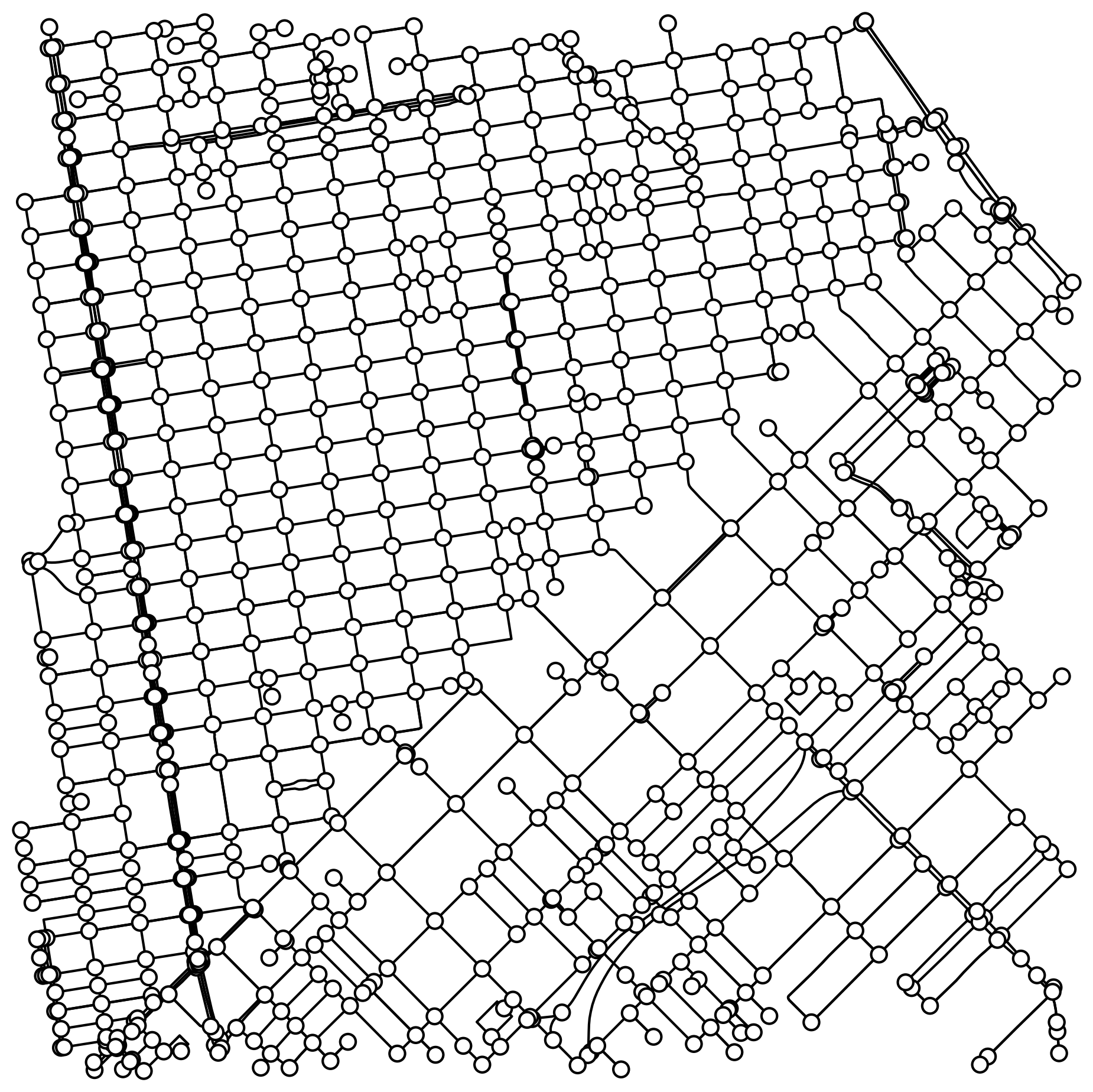
Figure 1: Street network used in numerical experiments

II-B Requests

We define a ride request $r$ as a tuple $r=\left<\rho_{r},\delta_{r},t_{r},\phi_{r}\right>$, where $\rho_{r}\in V$ and $\delta_{r}\in V$ correspond to the nearest intersection to the request’s desired pickup and drop-off locations, respectively; $t_{r}$ corresponds to the time at which the request was placed into the system; and $\phi_{r}\in\{0,1\}$ is an indicator, such that $\phi_{r}=1$ if the request has been picked up by a vehicle, $\phi_{r}=0$ otherwise. We model the number of requests that enter the system at time $t$ as a random variable $\eta_{t}$, which has the same distribution as random variable $\eta$ with an unknown underlying distribution $p_{\eta}$, which is fixed for the entire length of the time horizon $T$ and its estimated probability distribution, denoted $\tilde{p}_{\eta}$ is estimated from historical trip data. We denote the set of ride requests that enter the system at time $t$ as $\mathbf{r_{t}}$. Here the cardinality of the set of new requests at time $t$ is $|\mathbf{r_{t}}|=\eta_{t}$. We model the pickup intersection for an arbitrary request $r$ as the random variable $\rho_{r}$. Similarly, we model the drop-off intersection for request $r$ as the random variable $\delta_{r}$. We assume that requests are independent and identically distributed (i.i.d), and hence we drop the subscripts when talking about their distributions. Random variables $\rho$ and $\delta$ are jointly distributed and have unknown underlying probability distributions $p_{\rho}$ and $p_{\delta|\rho}$, respectively. These distributions do not change over the entire length of the time horizon $T$. We denote the marginal distribution of $\delta$ as $p_{\delta}$. We also denote the estimated categorical distributions for pickup locations, conditional dropoff locations, and the marginal dropoff locations as $\tilde{p}_{\rho}$, $\tilde{p}_{\delta|\rho}$, and $\tilde{p}_{\delta}$, respectively. These categorical distributions are estimated using historical trip data. We define $\mathbf{\overline{r}_{t}}=\{r|r\in\mathbf{r_{t^{\prime}}},\phi_{r}=0,1\leq t^{\prime}\leq t\}$ as the set of outstanding ride requests that have not yet been picked up by any taxi at time $t$.

II-C State and control space

We assume there is a total of $m$ taxis and all taxis can perfectly observe all requests, and other taxis’ locations and occupancy status through a central planner. We assume that all of the taxis remain inside the predefined street network $G$. We represent the state of the system at time $t$ as a tuple $x_{t}=\left<\vec{\nu_{t}},\vec{\tau_{t}},\mathbf{\overline{r}_{t}}\right>$. We define $\vec{\nu_{t}}=[\nu_{t}^{1},\dots,\nu_{t}^{m}]$ as the list of locations for all $m$ taxis at time $t$, where $\nu_{t}^{\ell}\in V$ corresponds to the index of the closest intersection to the geographical position of agent $\ell$. We define $\vec{\tau_{t}}=[\tau_{t}^{1},\dots,\tau_{t}^{m}]$ as the list of time remaining in current trip for all $m$ taxis. If agent $\ell$ is available, then it has not picked up a request and hence $\tau_{t}^{\ell}=0$, otherwise $\tau_{t}^{\ell}\in\mathds{N}^{+}$. The initial location of an arbitrary agent $\ell$ at time $t=0$ is given by random variable $\xi_{\ell}$. All $\xi_{\ell}$ for $\ell=1,\dots,m$ are assumed to be independent and identically distributed with known underlying distribution $p_{\xi}$.

We denote the control space for agent $\ell$ at time $t$ as $\mathbf{U}_{t}^{\ell}(x_{t})$. If the agent is available (i.e. $\tau_{t}^{\ell}=0$), then $\mathbf{U}_{t}^{\ell}(x_{t})=\{\mathcal{N}_{\nu_{t}^{\ell}},\nu_{t}^{\ell},\psi_{r}\}$, where $\psi_{r}$ corresponds to a special pickup control that becomes available if there is a request $r\in\mathbf{\overline{r}_{t}}$ with pickup at the location of agent $\ell$ (i.e. $\rho_{r}=\nu_{t}^{\ell}$). If the agent is currently servicing a request $r$ (i.e. $\tau_{t}^{\ell}>0$), then $\mathbf{U}_{t}^{\ell}(x_{t})=\{\zeta\}$, where $\zeta$ corresponds to the next hop in shortest path between agent $\ell$’s current location $\nu_{t}^{\ell}$ and the destination of the request $\delta_{r}$. Since this formulation represents a separable control space for each agent, the controls available to all $m$ taxis at time $t$, $\mathbf{U}_{t}(x_{t})$, is expressed as the Cartesian product of local control sets for each agent, such that $\mathbf{U}_{t}(x_{t})=\mathbf{U}_{t}^{1}(x_{t})\times\dots\times\mathbf{U}_{t}^{m}(x_{t})$.

II-D Stability of a policy

We define a policy $\pi=\{\mu_{1},\dots\mu_{T}\}$ as a set of functions that maps state $x_{t}$ into control $u_{t}=\mu_{t}(x_{t})\in\mathbf{U}_{t}(x_{t})$. Using a similar formulation as in [20], we define the total distance to be traveled in service of a request $r$ given a policy $\pi$ as $W_{r,\pi}=d(l_{r,\pi},\rho_{r})+d(\rho_{r},\delta_{r})$, where $l_{r,\pi}$ is the location of a taxi assigned to request $r$ based on policy $\pi$, and $d:V\times V\to\mathbb{N}^{+}$ is a function that gives the length of the shortest path between two locations. We define the total distance to be traveled in service of all the requests that enter the system for the entire time horizon $T$ as $Z_{\pi,T}=\sum_{t=1}^{T}\sum_{r=R_{t-1}+1}^{R_{t}}W_{r,\pi}$, where the random variable $R_{t}=\sum_{t^{\prime}=1}^{t}\eta_{t^{\prime}}$ represents the total number of requests that have entered the system until time $t$. It is important to note that $R_{0}=0$. We define the total distance that can be covered by a fleet of $m$ taxis as $m\cdot T$ since each agent can travel unit distance at each time step. Assuming that we have at least as many available taxis at each time step as incoming requests, a given policy $\pi$ is said to be stable if, for a fixed fleet size of $m$ taxis, the expected number of outstanding requests is uniformly bounded. Hence, a policy $\pi$ is stable as long as the distance to be traveled in service of all the requests that enter the system according to policy $\pi$ is smaller than the total distance that can be covered by a fleet of $m$ taxis. In other words, for a policy $\pi$ to be stable (following a similar argument as in [20]), the expected total distance for servicing all taxis should be upper bounded by the distance covered by taxis, i.e., $E[Z_{\pi,T}]<m\cdot T.$

II-E Challenges of a large scale multi-agent problem

We are interested in learning a cooperative pickup and routing policy on a city-scale map that minimizes the total wait time for all requests over a finite horizon of length $T$. We denote the state transition function as $f$, such that $x_{t+1}=f_{t}\left(x_{t},u_{t},\eta,\rho,\delta\right)$, where $x_{t+1}$ is the resulting state after control $u_{t}\in\mathbf{U}_{t}(x_{t})$ has been applied from state $x_{t}$. We define the stage cost $g_{t}\left(x_{t},u_{t},\eta,\rho,\delta\right)=|\mathbf{\overline{r}_{t}}|$ as the number of outstanding requests at time $t$. We denote the cost of executing policy $\pi$ as $J_{\pi}(x_{1})=E\left[g_{T}(x_{T})+\sum_{t=1}^{T-1}g_{t}\left(x_{t},\mu_{t}(x_{t}),\eta,\rho,\delta\right)\right]$, where $g_{T}(x_{T})=|\overline{\mathbf{r_{T}}}|$ is the terminal cost. Since the control space for the problem grows exponentially with the number of taxis, obtaining an optimal policy through the Bellman equations is intractable. For this reason, we consider policy improvement schemes, such as one-at-a-time rollout [13, 14], that allows us to obtain a lower cost policy by improving upon a base policy and it solves several smaller lookahead optimizations, one per agent, scaling linearly in the number of agents. We define base policy $\pi=\{{\mu}_{1},\dots\mu_{T}\}$ as an easy to compute heuristic that is given. One-at-a-time rollout finds an approximate policy $\tilde{\pi}=\{\tilde{\mu}_{1},\dots\tilde{\mu}_{T}\}$, where $\tilde{\mu}_{t}(x_{t})=(\tilde{\mu}^{1}_{t}(x_{t}),\ldots,\tilde{\mu}^{m}_{t}(x_{t}))$, $t=[1,\ldots,T]$. For state $x_{t}$, $\tilde{\mu}$ is found by solving $m$ minimizations starting from $\ell=[1,\ldots,m]$ as follows:

$$\tilde{\mu}^{\ell}_{t}(x_{t})\in\operatorname*{argmin}_{u^{\ell}_{t}\in\mathbf{U}^{\ell}_{t}(x_{t})}E[g_{t}(x_{t},u_{t},\eta,\rho,\delta)+\tilde{J}_{{\pi},t+1}(x_{t+1})],$$ (1)

where $u_{t}=(\tilde{\mu}^{1}_{t}(x_{t}):\tilde{\mu}^{\ell-1}_{t}(x_{t}),u_{t}^{\ell},{\mu}^{\ell+1}_{t}(x_{t}):{\mu}^{m}_{t}(x_{t}))$, and $\tilde{J}_{{\pi},t+1}(x_{t+1})=|\mathbf{\overline{r}_{t+1+t_{h}}}|+\sum_{t^{\prime}=t+1}^{t+t_{h}}g_{t^{\prime}}(x_{t^{\prime}},{\mu}_{t^{\prime}}(x_{t^{\prime}}),\eta,\rho,\delta)$ is a cost approximation derived from $t_{h}$ applications of the base policy ${\pi}$ from state $x_{t+1}$, with a terminal cost approximation $|\mathbf{\overline{r}_{t+1+t_{h}}}|$.

To apply one-at-a-time rollout to a large city-scale problem that scales linearly in the number of agents, we design an algorithm that approximates this rollout scheme, but incurs a lower computational cost that satisfy user defined computational constraints. Our algorithm is given in Sec. III. We must also find a sufficiently large fleet size $m$ for which a reasonable base policy $\pi$ is stable, such that $E[Z_{\pi,T}]<m\cdot T$, as defined in Sec. II-D. In particular, we are interested in the stability of the policy $\pi_{\text{base}}$ associated with IA-RA, as this policy is 2-competitive [16] and hence our approximate rollout approach obtains a near-optimal policy.

III Approximation algorithm for multiagent rollout

In this section we propose an approximate algorithm for multiagent rollout (see Section II-E, Eq. 1). Our proposed method is composed of a two-phase planning scheme that reduces the computational cost of one-at-a-time rollout through partitioning of the map using the demand distribution. We take into account user defined computational constraints in the form of the maximum number of taxis that can be run sequentially $m_{\text{lim}}$, and the length of the planning horizon $t_{h}$ (longer planning horizon result in longer runtimes). The algorithm is detailed in Algorithm 1. The proposed two-phase algorithm also takes as input $m$ the total number of taxis in the fleet. We provide theoretical bounds on $m$ in Sec. IV and calculated values in practice in Sec. V-C .

The first routine in Algorithm 1 is denoted as $get\_partitions$ to place the center of each partition on the map. $get\_partitions$ solves a capacitated facility location problem [21] on a deterministic multiagent matching problem where requests are sampled using a certainty equivalence approximation. The capacity for each partition center is set to be $m_{\text{lim}}$, and then the expected demand for the ride service during the entire time horizon is used as the demand for the capacitated facility location problem. The algorithm then assigns each node to the closest partition center using weighted $k$-means, where the weights of the nodes are given by the probability distribution of pickups. This routine guarantees that the size of each partition is then inversely proportional to the density of requests, and each partition is servicing an expected number of requests that can be served by the maximum number of taxis that can be run sequentially $m_{\text{lim}}$.

After obtaining the partitions, Algorithm 1 executes two routines at each time step: $High\_level\_planner$ (see Alg. 2), and $Low\_level\_planner$ (see Alg. 3). Intuitively, the $High\_level\_planner$ re-balances the taxis between partitions using an instantaneous assignment of taxis to current and expected future requests for the next $t_{h}$ time-steps as given by a certainty equivalence approximation. It returns the controls for taxis that are expected to go across regions $u_{h}^{g}$, as well as the list of high level taxis $\hat{m}$, and $\hat{d}$ the set of locations for the high level taxis to move towards. The $Low\_level\_planner$, on the other hand, plans for routing and pickup actions for taxis that remain in their original sectors according to the high level planner, executing one-at-a-time rollout with base policy IA-RA as defined in Eq. 1 to obtain $\tilde{u}_{t}^{k}$ the control of taxis in sector $k$ at time $t$.

After partitioning the graph, the state $x_{t}$ consists of $K$ sub-states $\{x^{k}_{t}\}_{k=1}^{K}$, one corresponding to a partition $k=\{1,\ldots,K\}$ of the graph. The state transition of partition $k$ is given by, $x^{k}_{t+1}=f^{k}(x^{k}_{t},u^{k}_{t},u^{g}_{h}(t,k),\eta,\rho,\delta).$ The control $u_{t}$ can be separated as $\{u^{k}_{t},u^{g}_{h}(t,k)\}_{k=1}^{K}$, where the control component $u^{k}_{t}$ corresponds to the taxis that are local to partition $k$. The control component $u^{g}_{h}(t,k)$ corresponds to the controls of taxis coming into partition $k$ as given by the higher level planner. Since we consider the length of outstanding requests as the stage cost, we have $|\mathbf{\overline{r}_{t}}|=g_{t}(x_{t},u_{t},\eta,\rho,\delta)=\sum_{k=1}^{K}g^{k}_{t}(x^{k}_{t},u^{k}_{t},u^{g}_{h}(t,k),\eta,\rho,\delta)=\sum_{k=1}^{K}|\mathbf{\overline{r}^{k}_{t}}|,$ where $\mathbf{\overline{r}^{k}_{t}}\subseteq\mathbf{\overline{r}_{t}}$, and $\forall r\in\mathbf{\overline{r}^{k}_{t}},\rho_{r}\in s_{k}$. The cost of our two-phase policy $\pi_{2P}$ is

$$J_{\pi_{2P}}(x_{t}) =E[\sum_{t^{\prime}=t}^{T}\sum_{k=1}^{K}g^{k}_{t^{\prime}}(x^{k}_{t^{\prime}},\tilde{u}^{k}_{t^{\prime}},u^{g}_{h}(t^{\prime},k),\eta,\rho,\delta)]$$

Input: Initial state $x_{1}$, maximum number of taxis per sector $m_{\text{lim}}$, fleet size $m$, planning horizon $t_{h}$

Output: policy $\pi_{2P}$ that gives routing/pickup strategy for all taxis in the system

1

2$K\leftarrow\frac{m}{m_{\text{lim}}}$

3$\{s_{k}\}_{k=1}^{K}\leftarrow get\_partitions(m_{\text{lim}},K,G,\eta,\rho,\delta)$

4$\hat{d}\leftarrow\{\},\hat{m}\leftarrow[]$

5for each time planning step $t\in[1,\dots,T]$ do

6      

7      $u^{g}_{h},\hat{m},\hat{d}\leftarrow High\_level\_planner(x_{t},\eta,\rho,\delta,$ $\pi_{\text{base}},t_{h},\hat{m},\hat{d},\{s_{k}\}_{k=1}^{K})$

8      for each sector $s_{k},k\in\{1,\ldots,K\}$ in parallel do

9             $\tilde{u}^{k}_{t}\leftarrow Low\_level\_planner(x^{k}_{t},u^{g}_{h}(t,k),\eta,\rho,$ $\delta,\pi_{\text{base}},t_{h},\hat{m},\hat{d})$

10      

11      set $\mu_{2P,t}(x_{t})=\{\tilde{u}^{k}_{t},u^{g}_{h}(t,k)\}_{k=1}^{K}$

12      $x_{t+1}\sim f(x_{t},\mu_{2P,t}(x_{t}),\eta,\rho,\delta)$

13set $\pi_{2P}=\{\mu_{2P,t}\}_{t=1}^{T}$

14return $\pi_{2P}$

Algorithm 1 Two-phase Planner

Input: $x_{t},\eta,\rho,\delta,\pi_{\text{base}},t_{h},\hat{m},\hat{d},\{s_{k}\}_{k=1}^{K}$

Output: control $u^{g}_{h}$ for taxis in $\hat{m}$, $\hat{m}$ the list of high level taxis, $\hat{d}$ the list of high level destinations for the high level taxis

1

2$r_{CE}\leftarrow$ list of $t_{h}\cdot E[\eta]$ future requests emulated by certainty equivalence for the next $t_{h}$ steps

3$A\leftarrow$ instantaneous assignment for the taxi set $\{\ell|\ell\in\{1,\ldots,m\},\tau_{\ell}=0\}$ to requests $\{\mathbf{\overline{r}_{t}}\cup r_{CE}\}$

4Define $sector(v)\in\{k|k\in\{1,\ldots,K\},v\in s_{k}\},\forall v\in V$

5Define $next\_hop\_in\_partition(v_{start},v_{end})\in\operatorname*{argmin}_{v\in s_{sector(v_{end})}\land v\in shortest\_path(v_{start},v_{end})}$ $d(v_{start},v)$, $\forall v_{start},v_{end}\in V,sector(v_{start})\neq sector(v_{end})$

6for each $(\ell,r)\in A,$ do

7      

8      if $sector(\nu_{\ell})\neq sector(\rho_{r})$ then

9            

10            $\hat{m}\leftarrow\hat{m}\cup\{\ell\}$,

11            $\hat{d}[\ell]\leftarrow next\_hop\_in\_partition(\nu_{\ell},\rho_{r})$

12      

13

14for each taxi $\ell\in\hat{m}$ do

15      

16      $u_{h}^{g}(t^{\prime},k)\leftarrow u_{h}^{g}(t^{\prime},k)\cup v,$ $|v\in shortest\_path(v_{\ell},\hat{d}[\ell])[t^{\prime}],v\in s_{k},0<t^{\prime}\leq d(v_{\ell},\hat{d}[\ell])$

17

18return $u^{g}_{h}$, $\hat{m}$, $\hat{d}$

Algorithm 2 High_level_planner

Input: $x^{k}_{t},u^{g}_{h}(t,k),\eta,\rho,\delta,\pi_{\text{base}},t_{h},\hat{m},\hat{d}$

Output: $\tilde{u}^{k}_{t}$

1

2Find taxis inside the sector $s_{k}$ as $m^{k}=\{\ell|\ell\in\{1,\ldots,m\},v_{\ell}\in s_{k},\ell\notin\hat{m}\}$

3Execute one-at-a-time rollout to obtain the control for each of the remaining taxis in $m^{k}$

4Starting from, $\ell=[1,\ldots,|m^{k}|]$

$$\tilde{u}^{k,m^{k}[\ell]}_{t}\in\operatorname*{argmin}_{u\in U_{t}^{m^{k}[\ell]}(x_{t}^{k})}E[g^{k}_{t}(x^{k}_{t},u^{\prime},u^{g}_{h}(t,k),\eta,\rho,\delta)$$ (2)

$$+\tilde{J}^{k}(x^{k}_{t+1})],$$

where $u^{\prime}=(\tilde{u}^{k,m^{k}[1]}_{t}:\tilde{u}^{k,m^{k}[\ell-1]}_{t}$,$u,u^{k,m^{k}[\ell+1]}_{base,t}:u^{k,m^{k}[|m^{k}|]}_{base,t})$ and $u^{k,\ell}_{base,t}$ is the control given by the base policy $\pi_{base}^{k}$ in the local state $x_{t}^{k}$, and the next state is $x^{k}_{t+1}=f^{k}(x^{k}_{t},u^{\prime},u^{g}_{h}(t,k),\eta,\rho,\delta)$ . The variable $\tilde{J}^{k}(x^{k}_{t+1})$ is the cost of applying the base policy $t_{h}$ times followed by a terminal cost approximation.

5return $\tilde{u}^{k}_{t}=[\tilde{u}^{k,m^{k}[1]}_{t},\ldots,\tilde{u}^{k,m^{k}[\ell]}_{t}]$

Algorithm 3 Low_level_planner

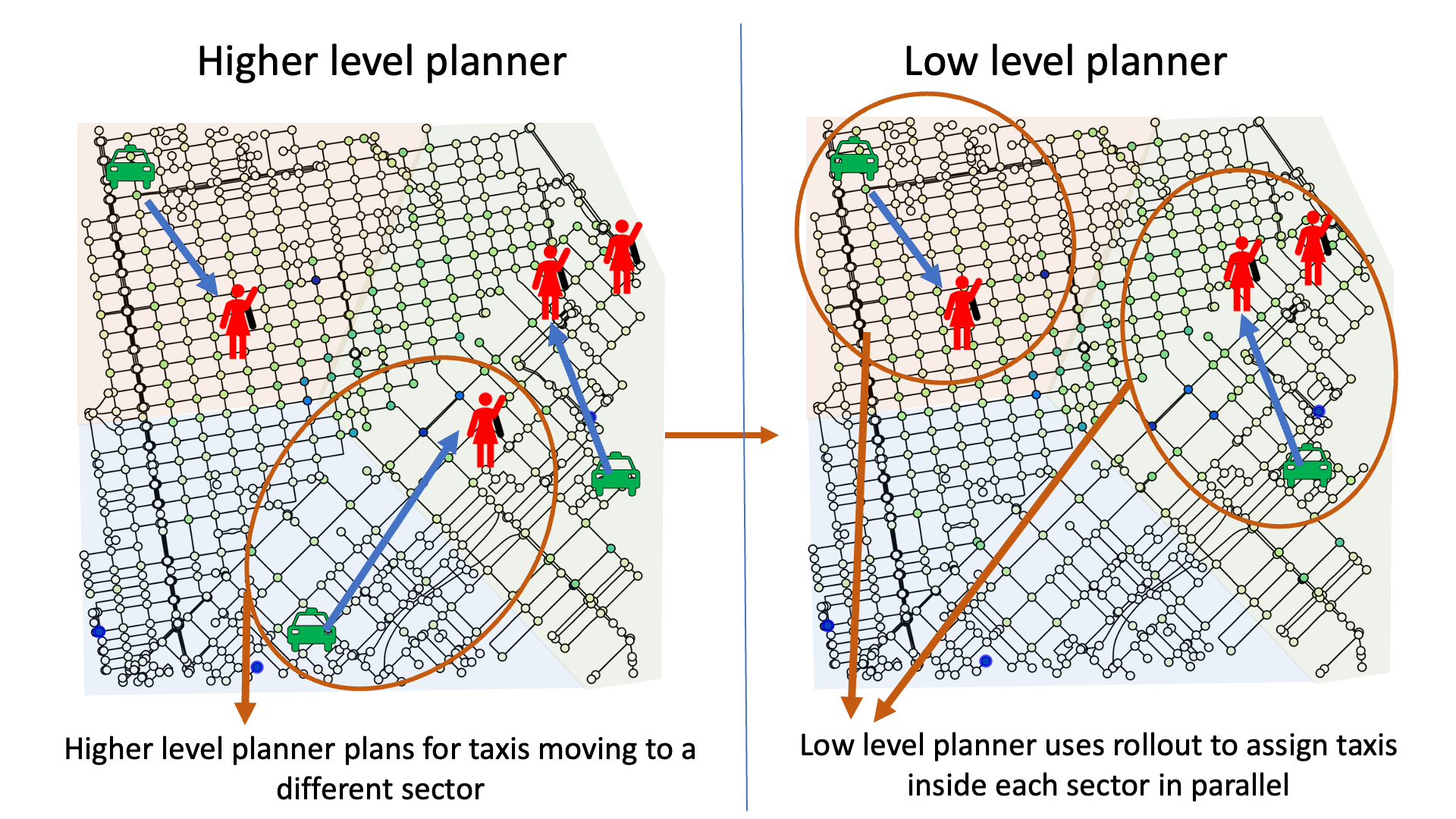
Figure 2: Two phased approach

Figure 2 shows the two phased approach with an example with $3$ taxis and $4$ outstanding requests.

IV Theoretical Results

In this section, we provide a sufficient condition for choosing a fleet size $m$ that will make the policy $\pi_{\text{base}}$, instantaneous assignment with reassignment (IA-RA), a stable policy. We also provide an asymptotic necessary condition on $m$ for the stability of $\pi_{\text{base}}$ as $T\to\infty$.

IV-A Sufficient condition for stability of $\pi_{\text{base}}$

We are interested in finding the sufficient conditions on the fleet size $m$ that guarantee the stability of policy $\pi_{\text{base}}$ such that the relation $E[Z_{\pi_{\text{base}},T}]<m\cdot T$ always holds. To do so, we first analyze the policy $\hat{\pi}$ referred to as random instantaneous assignment, where taxis are randomly assigned to requests. Under this policy, a taxi does not move until it has been assigned to a request. Once a taxi is assigned to a request, the taxi cannot be assigned to other requests until it has serviced the originally assigned request. By having a random assignment of requests to taxis, $l_{r,\hat{\pi}}$ for an arbitrary request $r$ becomes a random variable instead of a deterministic function of the requests in the system and the locations of all the taxis. The randomness in $\hat{\pi}$ also makes the request’s pickup location $\rho_{r}$ and the location of the taxi assigned to the request $l_{r,\hat{\pi}}$ independent, making the analysis easier. Using this policy, we can find an upper bound on $E[Z_{\hat{\pi},T}]$, and choose $m$ such that $m\cdot T$ is greater than the upper bound, making $\hat{\pi}$ a stable policy by definition. We then show that the policy $\pi_{\text{base}}$ given by a matching algorithm, like the auction algorithm [22] or the modified JVC algorithm [23], results in a smaller service distance than $\hat{\pi}$, i.e., $Z_{\pi_{\text{base}},T}\leq Z_{\hat{\pi},T}$. This implies $E[Z_{\pi_{\text{base}},T}]\leq E[Z_{\hat{\pi},T}]<m\cdot T$, and hence $\pi_{\text{base}}$ constitutes a stable policy for the sufficiently large fleet size $m$ found in the analysis of the stability of $\hat{\pi}$. We present the formal claim for the sufficient conditions on $m$ for the stability of $\hat{\pi}$ below in the following lemma.

Lemma 1

Let the random variable $l_{\text{rand}}$ with support $V$ represent the location of a random taxi that gets assigned to a request after that taxi has previously served a different request. Define $D_{\text{max}}\triangleq\max\{E[d(\xi,\rho)],E[d(l_{\text{rand}},\rho)]\}+E[d(\rho,\delta)]$. If the fleet size $m$ satisfies

$$m>E_{\eta}[\eta]\cdot D_{\text{max}},$$

then the policy associated with a random instantaneous assignment of taxis to requests, $\hat{\pi}$, constitutes a stable policy such that $E[Z_{\hat{\pi},T}]<m\cdot T$.

Proof:

First we rewrite $Z_{\hat{\pi},T}$ to consider the index of the requests irrespective of the time at which those requests enter the system. This allows us to get:

$$Z_{\hat{\pi},T}=\sum_{r=1}^{R_{T}}W_{r,\hat{\pi}}$$

where $R_{T}=\sum_{t=1}^{T}\eta_{t}$. Under the policy $\hat{\pi}$, a request is randomly assigned to a taxi. For this reason, there is a possibility that not all taxis in the fleet end up servicing a request. Hence, we define $\bar{m}$ as the random variable that corresponds to the effective fleet size over the entire time horizon, i.e., the number of taxis that pickup at least one request. We reindex requests such that requests that are assigned to taxis that haven’t serviced any requests come before requests that are assigned to taxis that have already serviced one or more requests. This means that the first $\bar{m}$ requests after reindexing are serviced by taxis that are still at their original initial locations. The rest of the requests are then serviced by taxis that are at the dropoff location of their previously serviced request. We can therefore, rewrite $Z_{\hat{\pi},T}$ as follows:

$$Z_{\hat{\pi},T}=\sum_{a=1}^{\bar{m}}W_{a,\hat{\pi}}+\sum_{b=\bar{m}+1}^{R_{T}}W_{b,\hat{\pi}}$$

Where, we have $W_{a,\hat{\pi}}=d(l_{a,\hat{\pi}},\rho_{a})+d(\rho_{a},\delta_{a})$. Similarly, $W_{b,\hat{\pi}}=d(l_{b,\hat{\pi}},\rho_{b})+d(\rho_{b},\delta_{b})$. The random variable $l_{a,\hat{\pi}}$ has the same distribution as $\xi$ since under $\hat{\pi}$ taxis are randomly matched to requests and taxis that haven’t been assigned to a request are still at their initial locations. Similarly, $l_{b,\hat{\pi}}$ has the same distribution as $l_{\text{rand}}$ since taxis are randomly matched to requests and taxis that have already serviced at least one request are located at the drop-off locations of their previously serviced request.

We define $W_{r_{\text{init}},\hat{\pi}}=d(l_{r_{\text{init},\hat{\pi}}},\rho_{r_{\text{init}}})+d(\rho_{r_{\text{init}}},\delta_{r_{\text{init}}})$, where $l_{r_{\text{init},\hat{\pi}}}$ is a random variable with the same distribution as $\xi$, $\rho_{r_{\text{init}}}$ is a random variable with the same distribution as $\rho$, and $\delta_{r_{\text{init}}}$ is a random variable with the same distribution as $\delta$. Now, we define $W_{r_{\text{next}},\hat{\pi}}=d(l_{r_{\text{next},\hat{\pi}}},\rho_{r_{\text{next}}})+d(\rho_{r_{\text{next}}},\delta_{r_{\text{next}}})$, where $l_{r_{\text{next},\hat{\pi}}}$ is a random variable with the same distribution as $l_{\text{rand}}$, $\rho_{r_{\text{next}}}$ is a random variable with the same distribution as $\rho$, and $\delta_{r_{\text{next}}}$ is a random variable with the same distribution as $\delta$. We can see that all $W_{a,\hat{\pi}}$ have the same distribution as $W_{r_{\text{init}},\hat{\pi}}$ since $W_{a,\hat{\pi}}$ is a function of three independent random variables $l_{a,\hat{\pi}},\rho_{a},$ and $\delta_{a}$ with the same distributions as $\xi,\rho$ and $\delta$, respectively. Similarly, all $W_{b,\hat{\pi}}$ have the same distribution as $W_{r_{\text{next}},\hat{\pi}}$ since $W_{b,\hat{\pi}}$ is a function of three independent random variables $l_{b,\hat{\pi}},\rho_{b},$ and $\delta_{b}$ with the same distributions as $l_{\text{rand}},\rho$ and $\delta$, respectively. Using these two facts, we will obtain an upper bound for $E[Z_{\hat{\pi},T}]$. Then, we set $m\cdot T$ to be greater than the upper bound to satisfy the definition of stability given in Sec. II-D. We consider the following:

$$E[Z_{\hat{\pi},T}] =E\left[\sum_{a=1}^{\bar{m}}W_{a,\hat{\pi}}+\sum_{b=\bar{m}+1}^{R_{T}}W_{b,\hat{\pi}}\right]$$

$$\overset{(1)}{=}E\left[E\left[\sum_{a=1}^{\bar{m}}W_{a,\hat{\pi}}\middle|\bar{m}\right]\right]$$

$$\qquad\qquad\qquad+E\left[E\left[\sum_{b=\bar{m}+1}^{R_{T}}W_{b,\hat{\pi}}\middle|R_{T},\bar{m}\right]\right]$$

$$\overset{(2)}{=}E\left[\sum_{a=1}^{\bar{m}}E[W_{a,\hat{\pi}}|\bar{m}]\right]$$

$$\qquad\qquad\qquad+E\left[\sum_{b=\bar{m}+1}^{R_{T}}E\left[W_{b,\hat{\pi}}\middle|R_{T},\bar{m}\right]\right]$$

$$\overset{(3)}{=}E\left[\sum_{a=1}^{\bar{m}}E[W_{r_{\text{init}},\hat{\pi}}]\right]+E\left[\sum_{b=\bar{m}+1}^{R_{T}}E\left[W_{r_{\text{next}},\hat{\pi}}\right]\right]$$

$$=E[\bar{m}]\cdot E[W_{r_{\text{init}},\hat{\pi}}]+E\left[(R_{T}-\bar{m})\cdot E\left[W_{r_{\text{next}},\hat{\pi}}\right]\right]$$

$$=E[\bar{m}]\cdot E[W_{r_{\text{init}},\hat{\pi}}]$$

$$\qquad\qquad\qquad+(E[R_{T}]-E[\bar{m}])\cdot E[W_{r_{\text{next}},\hat{\pi}}]$$

Where equality (1) comes from linearity of expectations and the law of total expectations; equality (2) comes from linearity of the conditional expectations; equality (3) comes from the fact that $W_{a,\hat{\pi}}$ is independent of $\bar{m}$, $W_{a,\hat{\pi}}$ has the same distribution as $W_{r_{\text{init}},\hat{\pi}}$, $W_{r_{b},\hat{\pi}}$ is independent of $R_{T}$ and $\bar{m}$, and $W_{r_{b},\hat{\pi}}$ has the same distribution as $W_{r_{\text{next}},\hat{\pi}}$ as explained before.

We can obtain an upper bound for $E[W_{r_{\text{init}},\hat{\pi}}]$ as follows:

$$E[W_{r_{\text{init}},\hat{\pi}}] \overset{(1)}{=}E[d(l_{r_{\text{init},\hat{\pi}}},\rho_{r_{\text{init}}})]+E[d(\rho_{r_{\text{init}}},\delta_{r_{\text{init}}})]$$

$$\overset{(2)}{=}E[d(\xi,\rho)]+E[d(\rho,\delta)]$$

$$\leq\max\{E[d(\xi,\rho)],E[d(l_{\text{rand}},\rho)]\}+E[d(\rho,\delta)]$$

$$\overset{(3)}{=}D_{\text{max}}$$ (3)

Where equality (1) comes from linearity of expectations, equality (2) comes from the definition of $W_{r_{\text{init}},\hat{\pi}}$, and equality (3) comes from the definition of $D_{\text{max}}$. Similarly, we can obtain an upper bound for $E[W_{r_{\text{next}},\hat{\pi}}]$ as follows:

$$E[W_{r_{\text{next}},\hat{\pi}}] \overset{(1)}{=}E[d(l_{r_{\text{next},\hat{\pi}}},\rho_{r_{\text{next}}})]+E[d(\rho_{r_{\text{next}}},\delta_{r_{\text{next}}})]$$

$$\overset{(2)}{=}E[d(l_{\text{rand}},\rho)]+E[d(\rho,\delta)]$$

$$\leq\max\{E[d(\xi,\rho)],E[d(l_{\text{rand}},\rho)]\}+E[d(\rho,\delta)]$$

$$\overset{(3)}{=}D_{\text{max}}$$ (4)

Where equality (1) comes from linearity of expectations, equality (2) comes from the definition of $W_{r_{\text{next}},\hat{\pi}}$, and equality (3) comes from the definition of $D_{\text{max}}$. Using these two results, we can upper bound $E[Z_{\hat{\pi},T}]$ as follows:

$$E[Z_{\hat{\pi},T}] \overset{(1)}{\leq}E[\bar{m}]\cdot D_{\text{max}}+(E[R_{T}]-E[\bar{m}])\cdot D_{\text{max}}$$

$$=E[R_{T}]\cdot D_{\text{max}}$$

$$\overset{(2)}{=}E\left[\sum_{t=1}^{T}\eta_{t}\right]\cdot D_{\text{max}}$$

$$\overset{(3)}{=}\sum_{t=1}^{T}E[\eta]\cdot D_{\text{max}}$$

$$=T\cdot E[\eta]\cdot D_{\text{max}}$$

where inequality (1) comes from and application of the upper bounds in Equation IV-A and Equation IV-A, equality (2) comes from the definition of $R_{T}$, and equality (3) comes from the linearity of expectations and the fact that variables $\eta_{t}$ are independent and identically distributed. From the stability definition given in Sec. II-D, $\hat{\pi}$ is stable as long as $E[Z_{\hat{\pi},T}]<m\cdot T$. Therefore, if we choose $m\cdot T>T\cdot E[\eta]\cdot D_{\text{max}}$ and hence $m>E[\eta]\cdot D_{\text{max}}$, this would be a sufficient condition to guarantee that the random instantaneous assignment policy $\hat{\pi}$ is stable such that the relation $E[Z_{\hat{\pi},T}]<m\cdot T$ holds. ∎

Notice that we can express the probability distribution $p_{l_{\text{rand}}}$ for $l_{\text{rand}}$ using the marginalization of the probabilities of the previous pickup-dropoff combinations, and hence all the terms given in $D_{\text{max}}$ can be calculated in practice using historical data. We use the result from lemma 1 to show that the same $m$ chosen to guarantee stability of $\hat{\pi}$ serves as a sufficiently large $m$ to guarantee stability of $\pi_{\text{base}}$ which is formalized in the Theorem 1.

Theorem 1

Assume that the fleet size $m$ satisfies the condition given in lemma 1. Then the policy $\pi_{\text{base}}$, which corresponds to standard instantaneous assignment with reassignment at each time step (IA-RA), is a stable policy such that $E[Z_{\pi_{\text{base}},T}]<m\cdot T$, for a finite horizon $T>0$.

Proof:

To prove this statement, we will show that random instantaneous assignment $\hat{\pi}$ results in longer distance traveled per assigned request than $\bar{\pi}$ standard instantaneous assignment with commitment to the initial assignment such that $Z_{\bar{\pi},T}\leq Z_{\hat{\pi},T}$. Then we will show that $\bar{\pi}$ results in longer distance traveled per assigned request than $\pi_{\text{base}}$ standard instantaneous assignment with reassignment at each time step such that $Z_{\pi_{\text{base}},T}\leq Z_{\bar{\pi},T}$. Since $\hat{\pi}$ is a stable policy for a fleet size of size $m>E[\eta]\cdot D_{\text{max}}$ according to lemma 1, and $Z_{\pi_{\text{base}},T}\leq Z_{\bar{\pi},T}\leq Z_{\hat{\pi},T}$, then we can conclude that $\pi_{\text{base}}$ is also stable since $E[Z_{\pi_{\text{base},T}}]\leq E[Z_{\bar{\pi},T}]\leq E[Z_{\hat{\pi},T}]<m\cdot T$.

We start by showing $Z_{\bar{\pi},T}\leq Z_{\hat{\pi},T}$. To do this, we consider the following:

$$Z_{\hat{\pi},T} \overset{(1)}{=}\sum_{t=1}^{T}\sum_{r=R_{t-1}+1}^{R_{t}}d(l_{r,\hat{\pi}},\rho_{r})+d(\rho_{r},\delta_{r})$$

$$\geq\sum_{t=1}^{T}\min_{l_{R_{t-1}+1},\dots,l_{R_{t}}}\sum_{r=R_{t-1}+1}^{R_{t}}d(l_{r},\rho_{r})+d(\rho_{r},\delta_{r})$$

$$\overset{(2)}{=}\sum_{t=1}^{T}\sum_{r=R_{t-1}+1}^{R_{t}}W_{r,\bar{\pi}}$$

$$\overset{(3)}{=}Z_{\bar{\pi},T}$$

Where equality (1) comes from the definition of $W_{r,\hat{\pi}}$, equality (2) comes from the definition of $\bar{\pi}$, and equality (3) comes from the definition of $Z_{\bar{\pi},T}$. This shows that $Z_{\bar{\pi},T}\leq Z_{\hat{\pi},T}$. From this, we get $E[Z_{\bar{\pi},T}]\leq E[Z_{\hat{\pi},T}]<m\cdot T$, and hence we can conclude that $\bar{\pi}$ is a stable policy for a fleet of size given by lemma 1.

To prove that $Z_{\bar{\pi},T}\geq Z_{\pi_{\text{base}},T}$, we will consider an argument for two arbitrary requests $r_{k}$ and $r_{h}$. We provide an argument with two requests for simplicity, but it is important to note that this argument can be easily generalized to as many requests as needed. The distance associated with the assignments produced by $\bar{\pi}$ is $W_{r_{k},\bar{\pi}}=d(l_{r_{k},\bar{\pi}},\rho_{r_{k}})+d(\rho_{r_{k}},\delta_{r_{k}})$ and $W_{r_{h},\bar{\pi}}=d(l_{r_{h},\bar{\pi}},\rho_{r_{h}})+d(\rho_{r_{h}},\delta_{r_{h}})$. We assume that request $r_{k}$ enter the system before request $r_{h}$, but request $r_{h}$ enter the system at time $t^{\prime}$ before the taxi assigned to request $r_{k}$ was able to pick request $r_{k}$ up. If we consider the time step $t^{\prime}$, policy $\bar{\pi}$ will match request $r_{h}$ to one of the taxis that hasn’t been assigned to any other request. Policy $\pi_{\text{base}}$, on the other hand, will perform a matching based on the distance from any available taxi to request $r_{h}$. In this sense, the original assignment given by $\bar{\pi}$ will be preserved unless a different assignment of free taxis to outstanding requests results in a lower distance. If we focus on the impact of the reassignment for these two requests at time $t^{\prime}$, we get:

$$Z_{\bar{\pi}} =W_{r_{k},\bar{\pi}}+W_{r_{h},\bar{\pi}}$$

$$\overset{(1)}{=}d(l_{r_{k},\bar{\pi}},\rho_{r_{k}})+d(\rho_{r_{k}},\delta_{r_{k}})+d(l_{r_{h},\bar{\pi}},\rho_{r_{h}})$$

$$\qquad\qquad\qquad\qquad\qquad\qquad\qquad+d(\rho_{r_{h}},\delta_{r_{h}})$$

$$\geq\min_{l_{r_{k}},l_{r_{h}}}d(l_{r_{k}},\rho_{r_{k}})+d(\rho_{r_{k}},\delta_{r_{k}})+d(l_{r_{h}},\rho_{r_{h}})$$

$$\qquad\qquad\qquad\qquad\qquad\qquad\qquad+d(\rho_{r_{h}},\delta_{r_{h}})$$

$$\overset{(2)}{=}W_{r_{k},\pi_{\text{base}}}+W_{r_{h},\pi_{\text{base}}}$$

$$\overset{(3)}{=}Z_{\pi_{\text{base}}}$$

where equality (1) comes from the definition of $W_{r_{k},\bar{\pi}}$ and $W_{r_{h},\bar{\pi}}$, equality (2) comes from the definition of $\pi_{\text{base}}$, and equality (3) comes from the definition of $Z_{\pi_{\text{base}},T}$.

From this, we can conclude $Z_{\bar{\pi},T}\geq Z_{\pi_{\text{base}},T}$, and hence $E[Z_{\pi_{\text{base}},T}]\leq E[Z_{\bar{\pi},T}]<m\cdot T$. Therefore, we can conclude that $\pi_{\text{base}}$ is a stable policy for a fleet size of $m$ as given by lemma 1. ∎

IV-B Necessary condition for stability of $\pi_{\text{base}}$

We are interested in finding the necessary condition for stability of policy $\pi_{\text{base}}$ asymptotically as $T\to\infty$. For this reason, we want to find a lower bound on $E[Z_{\pi_{\text{base}},T}/T]$. Choosing a fleet size $m$ smaller than this lower bound would make the policy $\pi_{\text{base}}$ asymptotically unstable, i.e., $E[Z_{\pi_{\text{base}},T}]\geq m\cdot T$ as $T\to\infty$. To obtain this result, we first find a lower bound for $E[Z_{\pi_{\text{base}},T}/T]$, the expected travel distance associated with servicing the requests that enter the system per time step, and then we apply a limit as $T\to\infty$ to obtain an expression for the asymptotic lower bound. The following theorem states this result formally.

Theorem 2

Let $\mathit{WD}(p_{\delta},p_{\rho})$ denote the first Wasserstein distance [24] between probability distributions $p_{\delta}$ and $p_{\rho}$ with support $\Omega$, such that:

$$\mathit{WD}(p_{\delta},p_{\rho})=\inf_{\gamma\in\Gamma(p_{\delta},p_{\rho})}\int_{x,y\in\Omega}||y-x||d\gamma(x,y),$$

where $||\cdot||$ is the euclidean metric, and $\Gamma(p_{\delta},p_{\rho})$ is the set of measures over the product space $\Omega\times\Omega$ having marginal densities $p_{\delta}$ and $p_{\rho}$, respectively. Define $D_{\text{min}}\triangleq\mathit{WD}(p_{\delta},p_{\rho})+E[d(\rho,\delta)]$. Assume that the random variables for pickups $\rho$ and drop-offs $\delta$ are independent and we have a fleet of size $m\leq E[\eta]\cdot D_{\text{min}}$. Then, the policy $\pi_{\text{base}}$ is asymptotically unstable, i.e., $E[Z_{\pi_{\text{base}},T}]\geq m\cdot T$ as $T\to\infty$.

Proof:

We denote $\pi_{\text{base}}$ as the policy that results from standard instantaneous assignment with rematching at each time step. We can rewrite $Z_{\pi_{\text{base}},T}$ as follows:

$$Z_{\pi_{\text{base}},T} =\sum_{r=1}^{R_{T}}W_{r,\pi_{\text{base}}}$$

where $R_{T}=\sum_{t=1}^{T}\eta_{t}$. We define $\bar{m}$ as the random variable that corresponds to the effective fleet size over the entire time horizon, i.e., the number of taxis that pickup at least one request, and we assume that this random variable is upper bounded by constant $m_{\text{cap}}$, which corresponds to the total number of taxis that can be deployed in our application. We reindex requests such that requests that are assigned to taxis that haven’t serviced any requests yet come before requests that are assigned to taxis that have already serviced one or more requests. This means that the first $\bar{m}$ requests after reindexing are serviced by taxis that were originally at their initial locations before any assignment. The rest of the requests are then serviced by taxis that were originally at the dropoff location of their previously serviced request before any assignment. We can therefore, rewrite $Z$ as follows:

$$Z_{\pi_{\text{base}},T} =\sum_{a=1}^{\bar{m}}W_{a,\pi_{\text{base}}}+\sum_{b=\bar{m}+1}^{R_{T}}W_{b,\pi_{\text{base}}}$$

Where, we have $W_{a,\hat{\pi}}=d(l_{a,\pi_{\text{base}}},\rho_{a})+d(\rho_{a},\delta_{a})$. Similarly, $W_{b,\hat{\pi}}=d(l_{b,\pi_{\text{base}}},\rho_{b})+d(\rho_{b},\delta_{b})$. Random variable $l_{a,\pi_{\text{base}}}$ depends on the distribution of initial locations of the taxis $p_{\xi}$, while random variable $l_{b,\pi_{\text{base}}}$ depends on the distribution of drop-offs for the requests $p_{\delta}$.

We are interested in finding an asymptotic lower bound for $E[Z_{\pi_{\text{base}},T}/T]$.We first consider:

$$E\left[\frac{Z_{\pi_{\text{base}},T}}{T}\right] \overset{(1)}{=}E\left[\frac{1}{T}\left(\sum_{a=1}^{\bar{m}}W_{a,\pi_{\text{base}}}+\sum_{b=\bar{m}+1}^{R_{T}}W_{b,\pi_{\text{base}}}\right)\right]$$

$$\overset{(2)}{=}E\left[E\left[\frac{1}{T}\sum_{a=1}^{\bar{m}}W_{a,\pi_{\text{base}}}\middle|\bar{m}\right]\right]$$

$$\qquad+E\left[E\left[\frac{1}{T}\sum_{b=\bar{m}+1}^{R_{T}}W_{b,\pi_{\text{base}}}\middle|R_{T},\bar{m}\right]\right]$$

$$\overset{(3)}{=}E\left[\frac{1}{T}\sum_{a=1}^{\bar{m}}E[W_{a,\pi_{\text{base}}}|\bar{m}]\right]$$

$$\qquad+E\left[\frac{1}{T}\sum_{b=\bar{m}+1}^{R_{T}}E\left[W_{b,\pi_{\text{base}}}\middle|R_{T},\bar{m}\right]\right]$$

Where equality (1) comes from the definition of $Z_{\pi_{\text{base}},T}$, equality (2) comes from linearity of expectations and the law of total expectations, and equality (3) comes from linearity of expectations and from the fact that given $R_{T}$ and $\bar{m}$, the conditional expectation can be moved inside the summation.

We define $\bar{d}_{\text{BMP}(\xi,\rho,\bar{m})}$ and $\bar{d}_{\text{BMP}(\delta,\rho,R_{T})}$ as the average lengths for the optimal solutions of the bipartite matching problem (BMP) for a fleet size of $\bar{m}$ and $R_{T}$ taxis, respectively, origins distributed according to probability distributions $p_{\xi}$ and $p_{\delta}$, respectively, and destinations distributed according to $p_{\rho}$. Similarly, we define $\bar{d}_{\text{EBMP}(\xi,\rho,\bar{m})}$ and $\bar{d}_{\text{BMP}(\delta,\rho,R_{T})}$ as the average lengths for the optimal solutions of the euclidean bipartite matching problem (EBMP) for a fleet size of $\bar{m}$ and $R_{T}$ taxis, respectively, origins distributed according to probability distributions $p_{\xi}$ and $p_{\delta}$, respectively, and destinations distributed according to $p_{\rho}$. Since $\bar{d}_{\text{BMP}(\xi,\rho,\bar{m})}$ is defined as the shortest path in the city graph between matched origins and destinations, we can easily see that this quantity can be lower bounded by $\bar{d}_{\text{EBMP}(\xi,\rho,\bar{m})}$ such that $\bar{d}_{\text{BMP}(\xi,\rho,\bar{m})}\geq\bar{d}_{\text{EBMP}(\xi,\rho,\bar{m})}$. Using this fact, we can lower bound $E[W_{a,\pi_{\text{base}}}|\bar{m}]$ as follows:

$$E[W_{a,\pi_{\text{base}}}|\bar{m}] \overset{(1)}{=}E[d(l_{a,\pi_{\text{base}}},\rho_{a})+d(\rho_{a},\delta_{a})|\bar{m}]$$

$$\overset{(2)}{=}E[d(l_{a,\pi_{\text{base}}},\rho_{a})|\bar{m}]+E[d(\rho,\delta)]$$

$$\overset{(3)}{\geq}\bar{d}_{\text{BMP}(\xi,\rho,\bar{m})}+E[d(\rho,\delta)]$$

$$\overset{(4)}{\geq}\bar{d}_{\text{EBMP}(\xi,\rho,\bar{m})}+E[d(\rho,\delta)]$$

$$=D_{\text{EBMP}}(\xi,\rho,\bar{m},\delta)$$ (5)

With $D_{\text{EBMP}}(\xi,\rho,\bar{m},\delta)\triangleq\bar{d}_{\text{EBMP}(\xi,\rho,\bar{m})}+E[d(\rho,\delta)]$. Equality (1) comes from the definition of $W_{a,\pi_{\text{base}}}$; equality (2) comes from linearity of expectations and the fact that $\rho_{a}$ and $\delta_{a}$ have the same distribution as $\rho$ and $\delta$, respectively, and they do not depend on $\bar{m}$; inequality (3) comes from the fact that since BMP assumes that all requests enter the system at time 0, obtaining a solution for this problem results in a smaller distance traveled than when requests enter the system at different time steps and hence taxis need to be reassigned; inequality (4) comes from the fact that $\bar{d}_{\text{BMP}(\xi,\rho,\bar{m})}\geq\bar{d}_{\text{EBMP}(\xi,\rho,\bar{m})}$ as explained above.

Similarly, we can lower bound $E\left[W_{b,\pi_{\text{base}}}\middle|R_{T},\bar{m}\right]$ for any $b>\bar{m}$ as follows:

$$E[W_{b,\pi_{\text{base}}}|R_{T},\bar{m}] \overset{(1)}{=}E[d(l_{b,\pi_{\text{base}}},\rho_{b})+d(\rho_{b},\delta_{b})|R_{T},\bar{m}]$$

$$\overset{(2)}{=}E[d(l_{b,\pi_{\text{base}}},\rho_{b})|R_{T},\bar{m}]+E[d(\rho,\delta)]$$

$$\overset{(3)}{\geq}\bar{d}_{\text{BMP}(\delta,\rho,R_{T}-\bar{m})}+E[d(\rho,\delta)]$$

$$\overset{(4)}{\geq}\bar{d}_{\text{EBMP}(\delta,\rho,R_{T}-\bar{m})}+E[d(\rho,\delta)]$$

$$=D_{\text{EBMP}}(\delta,\rho,R_{T}-\bar{m},\delta),$$ (6)

where $D_{\text{EBMP}}(\delta,\rho,R_{T}-\bar{m},\delta)=\bar{d}_{\text{EBMP}(\delta,\rho,R_{T}-\bar{m})}+E[d(\rho,\delta)]$. Equality (1) comes from the definition of $W_{b,\pi_{\text{base}}}$; equality (2) comes from linearity of expectations and the fact that $\rho_{b}$ and $\delta_{b}$ have the same distribution as $\rho$ and $\delta$, respectively, and they do not depend on $R_{T}$ or $\bar{m}$; inequality (3) comes from the fact that since BMP assumes that all requests enter the system at time 0, obtaining a solution for this problem results in a smaller distance traveled than when requests enter the system at different time steps and hence taxis need to be reassigned; inequality (4) comes from the fact that the euclidean distance is not constrained to the structure of the graph and hence $\bar{d}_{\text{BMP}(\delta,\rho,R_{T}-\bar{m})}\geq\bar{d}_{\text{EBMP}(\delta,\rho,R_{T}-\bar{m})}$.

Using these two lower bounds, we get:

$$E\left[\frac{Z_{\pi_{\text{base}},T}}{T}\right]$$

$$\overset{(1)}{\geq}E\left[\frac{1}{T}\sum_{a=1}^{\bar{m}}D_{\text{EBMP}}(\xi,\rho,\bar{m},\delta)\right]$$

$$\qquad+E\left[\frac{1}{T}\sum_{b=\bar{m}+1}^{R_{T}}D_{\text{EBMP}}(\delta,\rho,R_{T}-\bar{m},\delta)\right]$$

$$=E\left[\frac{\bar{m}}{T}D_{\text{EBMP}}(\xi,\rho,\bar{m},\delta)\right]$$

$$\qquad+E\left[\frac{1}{T}(R_{T}-\bar{m})D_{\text{EBMP}}(\delta,\rho,R_{T}-\bar{m},\delta)\right]$$

$$\overset{(2)}{=}E\left[\frac{\bar{m}}{T}D_{\text{EBMP}}(\xi,\rho,\bar{m},\delta)\right]$$

$$\qquad-E\left[\frac{\bar{m}}{T}D_{\text{EBMP}}(\delta,\rho,R_{T}-\bar{m},\delta)\right]$$

$$\qquad+E\left[\frac{1}{T}\left(\sum_{t=1}^{T}\eta_{t}\right)D_{\text{EBMP}}(\delta,\rho,R_{T}-\bar{m},\delta)\right]$$ (7)

where inequality (1) comes from the application of the bounds in Equation IV-B and Equation IV-B, and equality (2) comes from linearity of expectations and the definition of $R_{T}$.

Now, if we take the limit as $T\to\infty$ on both sides, we get the following:

$$\lim_{T\to\infty}E\left[\frac{Z_{\pi_{\text{base}},T}}{T}\right]$$

$$\overset{(1)}{\geq}\lim_{T\to\infty}[E\left[\frac{\bar{m}}{T}D_{\text{EBMP}}(\xi,\rho,\bar{m},\delta)\right]$$

$$\qquad-E[\frac{\bar{m}}{T}D_{\text{EBMP}}(\delta,\rho,R_{T}-\bar{m},\delta)]$$

$$\quad+E\left[\frac{1}{T}\left(\sum_{t=1}^{T}\eta_{t}\right)D_{\text{EBMP}}(\delta,\rho,R_{T}-\bar{m},\delta)\right]]$$

$$\overset{(2)}{\geq}\liminf_{T\to\infty}[E\left[\frac{\bar{m}}{T}D_{\text{EBMP}}(\xi,\rho,\bar{m},\delta)\right]$$

$$\qquad-E[\frac{\bar{m}}{T}D_{\text{EBMP}}(\delta,\rho,R_{T}-\bar{m},\delta)]$$

$$\quad+E\left[\frac{1}{T}\left(\sum_{t=1}^{T}\eta_{t}\right)D_{\text{EBMP}}(\delta,\rho,R_{T}-\bar{m},\delta)\right]]$$

$$\overset{(3)}{\geq}E\left[\liminf_{T\to\infty}\frac{\bar{m}}{T}D_{\text{EBMP}}(\xi,\rho,\bar{m},\delta)\right]$$

$$-E\left[\liminf_{T\to\infty}\frac{\bar{m}}{T}D_{\text{EBMP}}(\delta,\rho,R_{T}-\bar{m},\delta)\right]$$

$$+E\left[\liminf_{T\to\infty}\left(\sum_{t=1}^{T}\frac{\eta_{t}}{T}\right)D_{\text{EBMP}}(\delta,\rho,R_{T}-\bar{m},\delta)\right]$$

$$\overset{(4)}{=}E\left[\liminf_{T\to\infty}\left(\sum_{t=1}^{T}\frac{\eta_{t}}{T}\right)D_{\text{EBMP}}(\delta,\rho,R_{T}-\bar{m},\delta)\right]$$

$$\overset{(5)}{=}E[\eta]E\left[\liminf_{T\to\infty}D_{\text{EBMP}}(\delta,\rho,R_{T}-\bar{m},\delta)\right]$$

$$\overset{(6)}{\geq}E[\eta]\cdot(\mathit{WD}(p_{\delta},p_{\rho})+E[d(\rho,\delta)])$$

$$=E[\eta]\cdot D_{\text{min}}$$

where inequality (1) comes from the application of the limit to Equation IV-B; inequality (2) comes from the definition of $\liminf$; inequality (3) comes from the application of Fatou’s lemma; equality (4) comes from the fact that the first two terms go to zero as $T\to\infty$ since and $\bar{m}$ is upper bounded by a constant $m_{\text{cap}}$ and $D_{\text{EBMP}}$ is also upper bounded by a constant, more specifically the sum of $E[d(\rho,\delta)]$ and the generalized diameter of the euclidean region where the requests are being picked up; equality (5) comes from the law of large numbers which, since $\eta_{t}$ are i.i.d, results in $\liminf_{T\to\infty}\frac{1}{T}\left(\sum_{t=1}^{T}\eta_{t}\right)=E[\eta]$; inequality (6) comes from the analytical results presented in [19] where they show that $\liminf_{T\to\infty}D_{\text{EBMP}}(\delta,\rho,R_{T},\delta)\geq\mathit{WD}(p_{\delta},p_{\rho})+E[d(\rho,\delta)]$, where $\mathit{WD}(p_{\delta},p_{\rho})$ corresponds to the Wasserstein distance required to transform $p_{\delta}$ into $p_{\rho}$ distribution. This lower bound does no longer depend on $\eta$ or $\bar{m}$ and hence can be moved out of the expectation. The last equality comes from the definition $D_{\text{min}}\triangleq\mathit{WD}(p_{\delta},p_{\rho})+E[d(\rho,\delta)]$.

Now, we can finally conclude that $E\left[\frac{Z_{\pi_{\text{base}},T}}{T}\right]$ as $T\to\infty$ is lower bounded by $E[\eta]\cdot D_{\text{min}}$, and hence if $m\leq E[\eta]\cdot D_{\text{min}}$, the policy $\pi_{\text{base}}$ is asymptotically unstable since $m\cdot T\leq E\left[Z_{\pi_{\text{base}},T}\right]$ as $T\to\infty$. ∎

V Numerical studies

In this section we evaluate the performance of our algorithm using a real taxi data set for the city of San Francisco [25]. We compare the performance of our algorithm against three benchmarks: a greedy policy, instantaneous assignment with reassignment (IA-RA), and a rollout-based algorithm over the entire map as proposed in [12]. We provide a comparison of run-time of our two-phase approach and the rollout-based approach [12] to empirically verify the reduction in run-time associated with our two-phase approach. We verify our theoretical results in the number of taxis in the fleet required for stability by executing our algorithm for larger time horizons and plotting the number of outstanding requests at each time step. We empirically verify that for $m$ chosen in the range given by Theorem 1, and Theorem 2, our proposed approach is stable in the sense that the number of outstanding requests is uniformly bounded over time.

V-A Experimental Setup

Our numerical results consider a section of $1500m\times 1500m$ in San Francisco (see Fig. 1) with $859$ nodes and $1959$ edges. For the comparison studies we consider a horizon length of $T=60$, while for the stability results we consider $T=180$. All experiments were executed in an AMD Threadripper PRO WRX80. All individual results correspond to an average over 20 different trials with different instantiations of the random variables for the number of requests $\eta$, pickup locations $\rho,$, dropoff locations $\delta$, and the initial locations of the taxis $\xi$.

V-B Estimating probability distributions

For our experiments, we estimate $\tilde{p}_{\eta}$, $\tilde{p}_{\rho|\eta}$, and $\tilde{p}_{\delta}$ using historical trip data from several taxis in San Francisco [25]. We divide the historical data in 1-hour intervals, where each time step $t$ spans 1 minute. We empirically estimate $\tilde{p}_{\eta}$ by using the number of requests that arrive at each time step within each 1-hour time span. The distributions $\tilde{p}_{\rho}$ and $\tilde{p}_{\delta|\rho}$ are derived from the relative frequency of historical requests that originated and ended inside the map section. We estimate $\tilde{p}_{\delta|\rho}$ using relative frequency of pickup-dropoff pairs.

V-C Calculated values for theoretical results

For our experiments, we consider $\tilde{p}_{\eta}$ for an hour in which $E[\eta]=1$ (we get around $60$ requests per hour). For simplicity, we assume that $\xi$ is distributed according to the marginal probability distribution $p_{\delta}$, and hence we find that $E[d(\xi,\rho)]\approx 15$. We use $p_{l_{\text{rand}}}$ and $p_{\rho}$ to calculate $E[d(l_{\text{rand}},\rho)]\approx 13$. We use $p_{\rho}$ and $p_{\delta|\rho}$ to calculate $E[d(\rho,\delta)]\approx 15$. From this we get that the sufficient number of taxis for stability of our two-phase approach is $m>\max(15,13)+15=30$ from Theorem 1. We approximate the Wasserstein distance $\mathit{WD}(\delta,\rho)$ using the procedure suggested in [20]. We obtain $\mathit{WD}(\delta,\rho)\approx 1.87$. From this, we get that asymptotically, the minimum number of taxis needed for stability as $T\to\infty$ is $m>1.87+15$, rounding to next integer $m\geq 17$ from Theorem 2.

V-D Implementation details for two-phase approach

We execute $2000$ Monte-Carlo simulations with certainty equivalence to approximate the expected cost associated with each potential action in the one-step lookahead step of the rollout for the local planner. We also consider a planning horizon $t_{h}=10$ for the rollout, and a capacity of $m_{\text{lim}}=10$ taxis per sector, based on the computational resources available.

V-E Benchmarks

In this section, we discuss the details of the benchmarks to be used as comparisons for our performance results.

Greedy policy: Each taxi moves towards a request that is nearest to itself among all currently outstanding requests greedily, without coordinating with other taxis. This method does not consider future demand.

Instantaneous assignment (IA-RA): performs a deterministic matching of outstanding requests and available taxis without considering future requests. It solves a matching problem between available taxis and outstanding requests at every time step using an auction algorithm [26, 27].

One-at-a-time rollout-based global routing: performs rollout over the entire map using the procedure described in the scalability section of [12]. This method considers expected future demand.

V-F Performance results

This section includes the results for the performance and the execution time of our two-phase approach.

As shown in Fig. 3, our method results in a comparable performance to the rollout-based global routing [12]. For lower number of taxis, when $m<17$, our method is unstable. After we surpass $17$ taxis, standard IA-RA starts being stable for a larger proportion of the trials and our method starts performing similarly to the rollout-based global routing [12]. As shown in the graphs, for $m>30$, our proposed method results in a lower cost than IA-RA, resulting in a $5\%$ to $18\%$ improvement, sometimes even outperforming the rollout-based global routing thanks to the smaller sampling space associated with each sector. Since both rollout-based methods are running the same number of MC simulations, a smaller sample space leads to better approximation of the expectation.

To better understand the advantages of our proposed method, we compare the execution time of our proposed two-phase approach to the rollout-based global routing.

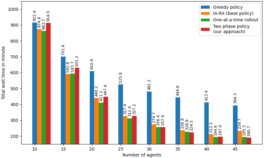
Figure 3: Total wait time over all requests of our two-phase approach and the benchmarks.

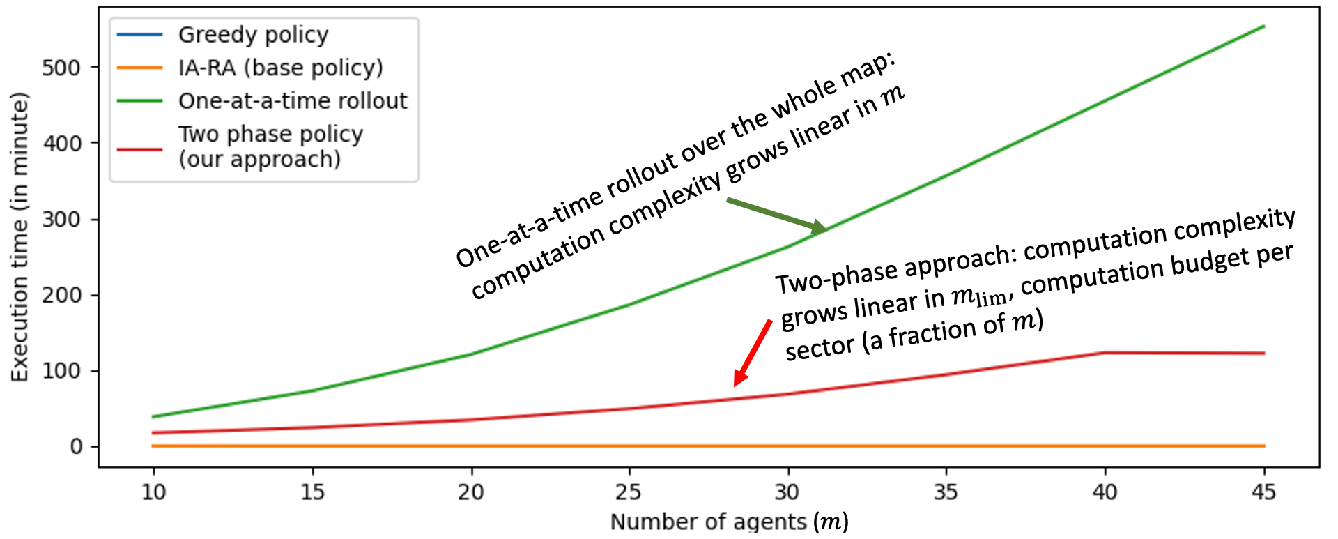
Figure 4: Execution time comparison of policies, including two-phase approach and one-at-a-time rollout over the entire map.

Fig. 4 shows our method results in significantly lower run-times than the rollout-based global routing, slowly increasing the execution time as the number of taxis in the fleet increases. The execution time eventually plateaus once the load in each sector becomes similar. This shows that partitioning the map and solving sub-problems in parallel results in a faster execution with similar total wait time to the global rollout.

V-G Stability of two-phase approach

Fig. 5 shows the stability results of our two-phase approach with various number of taxis over a horizon of 3 hours. Without enough taxis, $m<17$, for which the the IA-RA policy is shown to be unstable, our approach shows an increasing number of outstanding requests over time. However, with sufficient number of taxis ($m=25,35$), we see that both the IA-RA policy and our two-phase approach has a bounded number of outstanding requests over a large horizon of $180$ minutes.

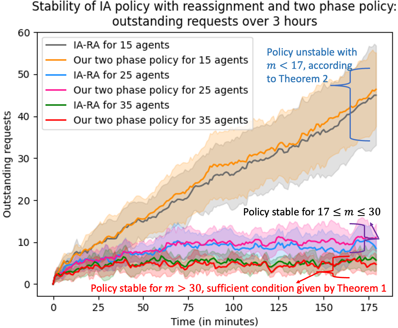
Figure 5: Stability in terms of the means (lines) and standard deviations (shared regions) of the number of outstanding requests for our two-phase policy and the IA-RA (base policy) over $3$ hours.

VI Conclusion

In this paper, we propose a multiagent scalable rollout-based two-phase algorithm for taxi pickup and routing problem on a large map and a large demand with a user-defined upper bound on the number of agents to plan for simultaneously. We provide a necessary and a sufficient conditions for the total fleet size $m$ to make the instantaneous assignment base policy stable, which is key to guarantee rollout’s convergence to a near-optimal policy. Our numerical results show that our two-phase approach approximates the standard one-at-a-time rollout with a much smaller computation cost when $m$ satisfies conditions calculated analytically. As future work, we want to tackle large urban mobility problems with changing traffic conditions.

References

• [1] N. Bidarian, “Regulators give green light to driverless taxis in san francisco,” CNN, 2023. [Online]. Available: https://www.cnn.com/2023/08/11/tech/robotaxi-vote-san-francisco/index.html
• [2] J. Muller, “Robotaxis hit the accelerator in growing list of cities nationwide,” Axios, 2023. [Online]. Available: https://www.axios.com/2023/08/29/cities-testing-self-driving-driverless-taxis-robotaxi-waymo
• [3] D. Kondor, I. Bojic, G. Resta, F. Duarte, P. Santi, and C. Ratti, “The cost of non-coordination in urban on-demand mobility,” Scientific Reports, vol. 12, 03 2022.
• [4] G. Berbeglia, J.-F. Cordeau, and G. Laporte, “Dynamic pickup and delivery problems,” European Journal of Operational Research, vol. 202, no. 1, pp. 8–15, 2010. [Online]. Available: https://www.sciencedirect.com/science/article/pii/S0377221709002999
• [5] R. Duan and S. Pettie, “Linear-time approximation for maximum weight matching,” J. ACM, vol. 61, no. 1, 2014. [Online]. Available: https://doi.org/10.1145/2529989
• [6] D. Bertsimas, P. Jaillet, and S. Martin, “Online vehicle routing: The edge of optimization in large-scale applications,” Oper. Res., vol. 67, pp. 143–162, 2019.
• [7] J. Alonso-Mora, A. Wallar, and D. Rus, “Predictive routing for autonomous mobility-on-demand systems with ride-sharing,” in 2017 IEEE/RSJ International Conference on Intelligent Robots and Systems (IROS).   IEEE, 2017, pp. 3583–3590.
• [8] M. Lowalekar, P. Varakantham, and P. Jaillet, “Online spatio-temporal matching in stochastic and dynamic domains,” Artificial Intelligence, vol. 261, pp. 71–112, 2018. [Online]. Available: https://www.sciencedirect.com/science/article/pii/S0004370218302030
• [9] R. Iglesias, F. Rossi, K. Wang, D. Hallac, J. Leskovec, and M. Pavone, “Data-driven model predictive control of autonomous mobility-on-demand systems,” in 2018 IEEE international conference on robotics and automation (ICRA).   IEEE, 2018, pp. 6019–6025.
• [10] D. Gammelli, K. Yang, J. Harrison, F. Rodrigues, F. Pereira, and M. Pavone, “Graph meta-reinforcement learning for transferable autonomous mobility-on-demand,” in Proceedings of the 28th ACM SIGKDD Conference on Knowledge Discovery and Data Mining, 2022, pp. 2913–2923.
• [11] T. Enders, J. Harrison, M. Pavone, and M. Schiffer, “Hybrid multi-agent deep reinforcement learning for autonomous mobility on demand systems,” in Learning for Dynamics and Control Conference.   PMLR, 2023, pp. 1284–1296.
• [12] D. Garces, S. Bhattacharya, S. Gil, and D. Bertsekas, “Multiagent reinforcement learning for autonomous routing and pickup problem with adaptation to variable demand,” in 2023 IEEE International Conference on Robotics and Automation (ICRA).   IEEE, may 2023.
• [13] D. Bertsekas, “Multiagent reinforcement learning: Rollout and policy iteration,” IEEE/CAA Journal of Automatica Sinica, vol. 8, no. 2, pp. 249–272, 2021.
• [14] ——, Rollout, Policy Iteration, and Distributed Reinforcement Learning, ser. Athena scientific optimization and computation series.   Athena Scientific., 2020. [Online]. Available: https://books.google.com/books?id=Hbo-EAAAQBAJ
• [15] ——, Lessons from AlphaZero for Optimal, Model Predictive, and Adaptive Control.   Nashua, NH, USA: Athena Scientific, 2022.
• [16] B. P. Gerkey and M. J. Matarić, “A formal analysis and taxonomy of task allocation in multi-robot systems,” The International journal of robotics research, vol. 23, no. 9, pp. 939–954, 2004.
• [17] R. Zhang and M. Pavone, “Control of robotic mobility-on-demand systems: A queueing-theoretical perspective,” The International Journal of Robotics Research, vol. 35, no. 1–3, p. 186–203, jan 2016. [Online]. Available: https://doi.org/10.1177/0278364915581863
• [18] M. Vazifeh, P. Santi, G. Resta, S. Strogatz, and C. Ratti, “Addressing the minimum fleet problem in on-demand urban mobility,” Nature, vol. 557, 05 2018.
• [19] K. Treleaven, M. Pavone, and E. Frazzoli, “Asymptotically optimal algorithms for one-to-one pickup and delivery problems with applications to transportation systems,” IEEE Transactions on Automatic Control, vol. 58, no. 9, pp. 2261–2276, 2013.
• [20] K. Spieser, K. Treleaven, R. Zhang, E. Frazzoli, D. Morton, and M. Pavone, “Toward a systematic approach to the design and evaluation of automated mobility-on-demand systems: A case study in singapore,” Road Vehicle Automation. Lecture Notes on Mobility, pp. 229–245, 04 2014.
• [21] L.-Y. Wu, X.-S. Zhang, and J.-L. Zhang, “Capacitated facility location problem with general setup cost,” Computers & Operations Research, vol. 33, no. 5, pp. 1226–1241, 2006. [Online]. Available: https://www.sciencedirect.com/science/article/pii/S0305054804002357
• [22] D. Bertsekas, “Constrained multiagent rollout and multidimensional assignment with the auction algorithm,” 2020. [Online]. Available: https://arxiv.org/abs/2002.07407
• [23] D. F. Crouse, “On implementing 2d rectangular assignment algorithms,” IEEE Transactions on Aerospace and Electronic Systems, vol. 52, no. 4, pp. 1679–1696, 2016.
• [24] L. Rüschendorf, “The wasserstein distance and approximation theorems,” Probability Theory and Related Fields, vol. 70, no. 1, pp. 117–129, 1985.
• [25] M. Piorkowski, N. Sarafijanovic-Djukic, and M. Grossglauser, “CRAWDAD dataset epfl/mobility (v. 2009-02-24),” Downloaded from https://crawdad.org/epfl/mobility/20090224, Feb. 2009.
• [26] D. Bertsekas, “A distributed algorithm for the assignment problem,” Lab. for Information and Decision Systems Report, 05 1979.
• [27] ——, Network Optimization: Continuous and Discrete Models, ser. Athena scientific optimization and computation series.   Athena Scientific, 1998. [Online]. Available: https://books.google.com/books?id=qUUxEAAAQBAJ