Euclid preparation

The Euclid photometric survey of galaxy clusters stands as a powerful cosmological tool, with the capacity to significantly propel our understanding of the Universe. Despite being sub-dominant to dark matter and dark energy, the baryonic component in our Universe holds substantial influence over the structure and mass of galaxy clusters. This paper presents a novel model to precisely quantify the impact of baryons on galaxy cluster virial halo masses, using the baryon fraction within a cluster as proxy for their effect. Constructed on the premise of quasi-adiabaticity, the model includes two parameters, which are calibrated using non-radiative cosmological hydrodynamical simulations, and a single large-scale simulation from the Magneticum set, which includes the physical processes driving galaxy formation. As a main result of our analysis, we demonstrate that this model delivers a remarkable one percent relative accuracy in determining the virial dark matter-only equivalent mass of galaxy clusters, starting from the corresponding total cluster mass and baryon fraction measured in hydrodynamical simulations. Furthermore, we also demonstrate that this result is robust against changes in cosmological parameters and against varying the numerical implementation of the sub-resolution physical processes included in the simulations. Our work substantiates previous claims about the impact of baryons on cluster cosmology studies. In particular, we show how neglecting these effects would lead to biased cosmological constraints for a Euclid-like cluster abundance analysis. Importantly, we demonstrate that uncertainties associated with our model, arising from baryonic corrections to cluster masses, are sub-dominant when compared to the precision with which mass-observable (i.e. richness) relations will be calibrated using Euclid, as well as our current understanding of the baryon fraction within galaxy clusters.

1 Introduction

In the $\Lambda$CDM scenario, structures are formed hierarchically, with larger systems emerging from the merger of smaller ones. As the largest, most massive, virialized objects in the Universe, galaxy clusters are at the pinnacle of this hierarchy and provide competitive cosmological probes of the geometry of our Universe and of the growth of density perturbations through measurements of their cosmic abundance and clustering (see, e.g., Allen et al. 2011; Kravtsov & Borgani 2012; Fumagalli et al. 2023).

While structure formation is gravitationally dominated by dark matter, astrophysical effects associated with the baryonic component are known to significantly affect the clusters and cluster galaxy population  (see, for example, McDonald et al. 2012; Webb et al. 2015; Ellien et al. 2019; Schellenberger et al. 2019; Yuan et al. 2020; Debackere et al. 2021). In this context, advanced cosmological simulations (e.g., Borgani & Kravtsov 2011) provide the best tools for studying the formation of galaxy clusters starting from primordial density perturbations.

The primary cosmological probe from cluster surveys comes from number-count experiments (Borgani et al. 2001; Holder et al. 2001; Rozo et al. 2010; Hasselfield et al. 2013; Planck Collaboration XX. 2014; Bocquet et al. 2015; Mantz et al. 2015; Planck Collaboration XXIV. 2016; Bocquet et al. 2019; Abbott et al. 2020; Costanzi et al. 2021; Lesci et al. 2022), which rely on the strong cosmological dependence of volumes and of the halo mass function (HMF) – the density of halos as a function of mass and redshift.

The prediction of the HMF relies deeply on the results of cosmological simulations (see, for instance, Tinker et al. 2008; Watson et al. 2013; Bocquet et al. 2016; Despali et al. 2016; Castro et al. 2020; Bocquet et al. 2020; Euclid Collaboration: Castro et al. 2023). Since simulations involving full hydrodynamical calculations are prohibitively more expensive than purely gravitational $N$-body simulations, the conventional method is to characterize the HMF using the latter and model how baryonic physics alters the mass of halos in post-processing (Schneider & Teyssier 2015; Aricò et al. 2021). For the sake of brevity, we shall henceforth refer to these hydrodynamical simulations simply as ‘hydro’ and their dark-matter (DM) only $N$-body counterpart as ‘dmo’. As already mentioned, despite being sub-dominant, the baryonic component has a sizeable impact on the detailed properties of the large-scale structure of our Universe (Cui et al. 2014; Velliscig et al. 2014; Bocquet et al. 2016; Castro et al. 2018, 2020; Schaye et al. 2023).

Feedback processes related to supernovae (SN) and to active galactic nuclei (AGN) originate on small scales that cannot be explicitly resolved in simulations covering large cosmological volumes. As a result, it is impossible to explicitly simulate these processes within such large volumes from first principles; instead, sub-resolution models must be used (e.g., Springel & Hernquist 2003; Hirschmann et al. 2014; Vogelsberger et al. 2014; Schaye et al. 2015; Crain et al. 2015; McCarthy et al. 2017; Vogelsberger et al. 2020). These processes, however, affect the distribution of baryons and cosmic structures on scales well resolved by cosmological simulations and probed by observations (see, e.g., van Daalen et al. 2011).

The strategy to describe such processes in simulations through sub-resolution phenomenological models has offered invaluable insights into quantifying the influence of baryonic effects on large-scale structure (see, e.g., Teyssier et al. 2011; van Daalen et al. 2011; Martizzi et al. 2013; Sawala et al. 2016; Bullock & Boylan-Kolchin 2017; van Daalen et al. 2020; Schaye et al. 2023). However, due to our incomplete understanding of the associated sub-resolution physical processes, several of the parameters used in their implementation require a calibration to reproduce some key observables. This calibration is usually carried out for one or few specific observables, and is intrinsically resolution-dependent (see Schaye et al. 2015, for discussion). Furthermore, due to the complex interaction and the degeneracy between highly non-linear processes, different choices for such parameters can equally reproduce the target observables.

It is established that at the scales relevant for galaxy clusters, baryonic feedback cannot disrupt structures. However, various astrophysical processes associated with the baryonic component can still alter the halo mass. Specifically, these processes include radiative cooling and star-formation, both of which can induce adiabatic contraction of the halo. Moreover, sudden displacement of gas caused by impulsive AGN feedback can lead to an expansion of the halo. These dynamic processes significantly modify the halo mass when compared to the same halo described within a dmo simulation  (see, for instance, Velliscig et al. 2014; Castro et al. 2020). In this light, a comprehensive understanding of such influences is indispensable for accurate modelling and interpretation of hydro simulations.

In this paper, we model the impact on the halo virial mass caused by baryonic effects. Our model assumes that the processes involved are quasi-adiabatic, i.e., they happen in a steady, non-abrupt manner. Although our model is calibrated on a set of non-radiative hydro simulations and on a single realization of a full-physics simulation, its performance will be demonstrated to be robust against the change of parameters controlling the sub-resolution physics as well as against choosing independent implementations of sub-resolution processes.

The large statistics of clusters that will be provided by Euclid (Laureijs et al. 2011) cluster survey require a high-precision calibration of the HMF, so that uncertainties on this theory-predicted quantity do not represent the limiting factor in the precision achievable by the cluster survey (see Euclid Collaboration: Adam et al. 2019). In Euclid Collaboration: Castro et al. (2023), we used a large set of $N$-body simulations to derive an analytical, cosmology-dependent expression for the HMF that meets the required precision of $\simeq 1$ percent. In this paper, we extend the results of our previous work to account for baryonic effects. Our goal is thus to reach a one percent accuracy on the baryonic impact description, to match the Euclid requirements to fully exploit the cosmological constraining power of the Euclid cluster survey (Sartoris et al. 2016).

This paper is organized as follows: we outline the methodology used in this paper in Sect. 2. In Sect. 3, we present the findings from the simulations and the performance of the baryonic correction model. In Sect. 4, we assess the impact of our model in a forecast Euclid cluster count analysis. Final remarks are made in Sect. 5. Lastly, in Appendix A, we study the baryonic content in different simulations.

2 Methodology

2.1 Simulations

In this section, we describe the simulations that are used to calibrate the baryonic effects on halo masses, and the preparation of the halo catalogs to compare results from hydro and dmo simulations.

2.1.1 The Magneticum set

The Magneticum simulations were carried out using the TreePM+SPH code P-Gadget3, which is a more efficient variation of Gadget-2 (Springel et al. 2001b; Springel 2005). The SPH solver uses the revised implementation of Beck et al. (2016), which overcomes a number of limitations of the traditional SPH solvers. The Magneticum hydro simulations include treatment of radiative cooling, heating by a uniform evolving UV background, star-formation and stellar feedback following Springel et al. (2005), and the description of stellar evolution and chemical enrichment processes by Tornatore et al. (2007). According to the latter, eleven chemical elements are followed, once produced by AGB stars, Type-Ia SN, and Type-II SN (H; He; C; N; O; Ne; Mg; Si; S; Ca; Fe). Following Wiersma et al. (2009), metallicity-dependent cooling is implemented using cooling tables generated by the freely accessible CLOUDY photo-ionization algorithm (Ferland et al. 1998). Super-massive black holes, hosted at the center of galaxies, are described as sink particles whose mass increases by gas accretion and merging with other BHs  (Springel et al. 2005; Di Matteo et al. 2008). Accretion onto these black holes is governed by the Bondi-Hoyle-Lyttleton formula (Hoyle & Lyttleton 1939; Bondi & Hoyle 1944; Bondi 1952), capped by the Eddington rate, and involves both quasar- and radio-mode feedback regimes. Further details on the specific model of gas accretion and the AGN feedback are provided in Hirschmann et al. (2014). The Magneticum set also counts with the dmo counterpart for every hydro simulation and a few non-radiative simulations. The non-radiative simulations include gas hydrodynamics but no other sub-resolution physics.

In Table 1, we report the relevant parameters regarding box size and mass resolution of the subset of Magneticum simulations we use as reference for our analysis. While the reference cosmology of the Magneticum simulations is WMAP7  (Komatsu et al. 2011), for the largest box here considered, Box 1a, the Magneticum suite also covers different cosmologies as presented in Table 2 (see also Singh et al. 2020). Although cosmological parameters are varied, all these simulations keep the relevant parameters describing the sub-resolution models fixed. In addition, we also include $4$ simulations that either vary the AGN feedback efficiency by $\pm 33$ percent, or assume a wind velocity of $500$ or $800$ ${\rm km\,s}^{-1}$, instead of the fiducial value of $350$ ${\rm km\,s}^{-1}$.

Table 1: Set of boxes from Magneticum simulations and halo selection parameters used in this work. Column 1: name of the boxes; Column 2: size of the simulation box; Column 3: mass of the DM particle in each box; Column 4: minimum mass of the halos considered in our analysis; Column 5: the different physical models used to run the simulations.

Box	$L_{\textrm{box}}$	$m_{\textrm{DM}}$	$M_{\textrm{halo},\textrm{min}}$	Physics
	$(\textrm{Mpc})$	($M_{\odot}$)	($M_{\odot}$)	hydro	dmo	non-radiative
2	$500$	$9.8\times 10^{8}$	$4.3\times 10^{13}$	✓	✓
2b	$909$	$9.8\times 10^{8}$	$4.3\times 10^{13}$	✓	✓
1a	$1272$	$1.9\times 10^{10}$	$4.3\times 10^{14}$	✓	✓	✓

Table 2: Set of cosmologies covered by Magneticum Box 1a simulations used in this work.

Name	$\Omega_{\rm m}$	$\sigma_{8}$	$h$	$f_{\rm b}$	Physics
					hydro	dmo	non-radiative
$C1$	$0.153$	$0.614$	$0.666$	$0.267$	✓	✓	✓
$C2$	$0.189$	$0.697$	$0.703$	$0.241$	✓	✓
$C3$	$0.204$	$0.739$	$0.689$	$0.214$	✓	✓
$C4$	$0.200$	$0.850$	$0.730$	$0.208$	✓	✓
$C5$	$0.222$	$0.793$	$0.676$	$0.190$	✓	✓
$C6$	$0.232$	$0.687$	$0.670$	$0.178$	✓	✓
$C7$	$0.268$	$0.721$	$0.699$	$0.168$	✓	✓
$C8$	$0.272$	$0.809$	$0.704$	$0.168$	✓	✓	✓
$C9$	$0.304$	$0.886$	$0.740$	$0.166$	✓	✓
$C10$	$0.301$	$0.834$	$0.708$	$0.153$	✓	✓
$C11$	$0.342$	$0.834$	$0.708$	$0.135$	✓	✓
$C12$	$0.363$	$0.884$	$0.729$	$0.135$	✓	✓
$C13$	$0.400$	$0.650$	$0.675$	$0.121$	✓	✓
$C14$	$0.406$	$0.867$	$0.712$	$0.115$	✓	✓
$C15$	$0.428$	$0.830$	$0.732$	$0.115$	✓	✓	✓

2.1.2 Illustris TNG

The Illustris TNG simulations were run using the AREPO code (Springel 2010), which has a gravity solver similar to the P-Gadget3 one, with a hydro solver based on solving the Riemann problem on a moving mesh. This set of simulations represents an improvement in terms of the sub-resolution models adopted for star-formation and feedback models, with respect to those adopted in the original Illustris simulations (Vogelsberger et al. 2013). It makes use of the same galaxy formation model with an improved kinetic AGN feedback model, a new parameterization of galactic winds, and the addition of magnetic fields (see, Weinberger et al. 2017; Pillepich et al. 2018; Pakmor et al. 2011; Pakmor & Springel 2013; Pakmor et al. 2014, respectively).

For the purpose of the analysis presented in this paper, we use the largest box available, i.e. the TNG-300 and its dmo counterpart. The simulated box size is $302.6$ Mpc and has a DM particle mass of $5.9\times 10^{7}\,M_{\odot}$, the assumed cosmological model being that of Planck 2015  (Planck Collaboration XIII. 2016). We select all halos with mass higher than $1.0\times 10^{13}\,M_{\odot}\,h^{-1}$.

2.1.3 Halo catalogs

The halo catalogs used in this paper were obtained by using the SUBFIND halo finder (Springel et al. 2001a, 2021), as presented in Dolag et al. (2009). This version of the code includes also gas and star particles. SUBFIND starts by establishing halo centers by running a parallel implementation of the 3D friends-of-friends (FOF; see, for instance, Davis et al. 1985) algorithm and then allocating it to the position of the particle with the lowest potential. After that, it grows spheres around the center and calculates the mass inside several radii, including a mean density $\Delta$ times the cosmic critical density. Throughout this paper, we only refer to the quantities with respect to the virial overdensity, $\Delta_{\rm vir}$, computed for the corresponding cosmology (see, Bryan & Norman 1998).

2.1.4 Matching algorithm

For the purpose of the analysis presented in this paper, we need to identify the halo pairs corresponding to the same object identified in a hydro simulation and in its dmo counterpart. The matched catalogs are created by detecting the halo pairs from each of the hydro and dmo runs that are the closest to each other. Pairs that had a difference in mass larger than $50$ percent were discarded. The same procedure was applied by Castro et al. (2020), stating that the matched catalog completeness and purity are greater than $95$ percent for objects more massive than a few times $10^{13}\,M_{\odot}$. We have independently validated the performance of the matching algorithm by comparing this position-based matching algorithm with a stricter matching algorithm based on matching objects that share more than $50$ percent of the DM particles.

2.2 Baryonic correction on halo masses

The baryonic component can impact the spherical overdensity mass of galaxy clusters in three ways: due to adiabatic contraction, baryonic feedback, and the different dynamics between baryonic matter and DM. The adiabatic contraction is induced by radiative cooling of the diffuse gas. As the gas loses energy, its pressure support diminishes, leading to a fast collapse towards the bottom of the potential well, which in turn reacts by slightly contracting (e.g., Gnedin et al. 2004). This contraction is modulated by the rate of gas cooling.

Concerning the feedback effects, these can cause sudden gas heating, and its subsequent displacement by expansion. Consequently, the DM halo responds by slightly expanding, with the extent of expansion depending on the intensity of feedback. While feedback associated with SN has been shown in simulations not to efficiently counteract adiabatic contraction on the scales of galaxy clusters and groups, AGN feedback is able to displace a large amount of gas. Subsequently, the overall structure of the cluster is affected as the DM component is passively dragged by the baryonic component.

Lastly, another baryonic effect is the difference in accretion dynamics between DM and gas, with baryonic matter experiencing slower accretion due to the presence of shocks. This differential accretion can also affect the overall structure and mass of the galaxy clusters.

If baryonic effects happen slowly with respect to the cluster dynamical time and orbits are spherically symmetric, the angular momentum is an adiabatic invariant of the mass enclosed by the collapsing shell, leading to the conservation of the quantity $M(R)\,R$, where $M(R)$ is the total mass inside the radius $R$ (see, for intance, Steigman et al. 1978; Zeldovich et al. 1980; Blumenthal et al. 1986; Ryden & Gunn 1987). Thus, for a cluster-sized halo produced in the hydrodynamic simulation, having virial mass $M_{\textrm{vir},\textrm{hyd}}$ and virial radius $R_{\textrm{vir},\textrm{hyd}}$ we can write

$$M_{\Delta,{\rm dmo}}\,R_{\Delta,{\rm dmo}}=M_{\textrm{vir},\textrm{hyd}}\,R_{\textrm{vir},\textrm{hyd}}\,,$$ (1)

where $M_{\Delta,{\rm dmo}}$ is the mass contained inside the sphere of radius $R_{\Delta,{\rm dmo}}$ centered on the dmo counterpart not affected by the baryonic physics. Note that, due to the baryonic impact on the halo profile, the overdensity threshold $\Delta$ in general will differ from the virial value. Defining $f_{\textrm{b},\textrm{cosmic}}$ as the cosmic baryon fraction and $f_{\textrm{b},\textrm{vir}}$ as the baryon fraction within the halo virial radius, then

$$M_{\Delta,{\rm dmo}}=\frac{1-f_{\textrm{b},\textrm{vir}}}{1-f_{\textrm{b},\textrm{cosmic}}}\,M_{\textrm{vir},\textrm{hyd}}\,.$$ (2)

The above equation follows from the fact that the DM mass in the hydro-simulated halo – i.e. $(1-f_{\rm b,vir})\,M_{\rm vir,hyd}$ – should correspond to a mass $(1-f_{\rm b,cosmic})^{-1}$ times larger than in the dmo counterpart, which by definition is only made by a collisionless component. From Eqs. (1) and (2) it follows that

$$\frac{R_{\Delta,{\rm dmo}}}{R_{\rm vir,hyd}}=\frac{1-f_{\rm b,cosmic}}{1-f_{\rm b,vir}}\,,$$ (3)

and the overdensity $\Delta$ is defined as

$$\Delta=\frac{3\,M_{\Delta,{\rm dmo}}}{4\,\pi\,R_{\Delta,{\rm dmo}}^{3}\,\rho_{\rm c}}\,,$$ (4)

with $\rho_{\rm c}=3H^{3}/(8\pi G)$ the cosmic critical density and $H$ the Hubble parameter.

Several papers studied the validity of the adiabatic approximation for the halo profile (see, for example, Jesseit et al. 2002; Gnedin et al. 2004; Duffy et al. 2010; Velmani & Paranjape 2023), showing that several of the assumptions made are violated; for instance, orbits can deviate strongly from sphericity, due to major mergers. Furthermore, energy feedback effects can result in abrupt injection of gas kinetic energy in the cluster core, thus violating the quasi-static assumption. To take these effects into account, we modify Eqs. (2) and (3) as:

$$M_{\Delta,{\rm dmo}} =\frac{1-f_{\rm b,vir}-\delta_{f}}{1-f_{\rm b,cosmic}}\,M_{\rm vir,hyd}\,,$$ (5)

$$\frac{R_{\Delta,{\rm dmo}}}{R_{\rm vir,hyd}} =1+q\,\left(\frac{1-f_{\rm b,cosmic}}{1-f_{\rm b,vir}-\delta_{f}}-1\right)\,,$$ (6)

where $q$ is a quasi-adiabatic parameter, which controls the deviation from the adiabatic assumption (see, Schneider & Teyssier 2015; Paranjape et al. 2021), and $\delta_{f}$ accounts for the baryonic off-set, for which a halo containing $f_{\rm b,vir}=f_{\rm b,cosmic}-\delta_{f}$ has the same mass as its dmo counterpart. Note that zero correction corresponds to $\delta_{f}=0$ and $q=1$. It is important to emphasize that these two parameters, $q$ and $\delta_{f}$, both require to be calibrated against simulations. This calibration is addressed in the following sections.

In summary, to derive the reconstructed dmo virial mass we follow these steps:

1. For a given mass $M_{\rm vir,hyd}$ we calculate the $M_{\rm\Delta,dmo}$ using Eq. (5);

2. We calculate $R_{\Delta,\rm dmo}$ using Eq. (6);

3. The dmo spherical overdensity threshold $\Delta$ is calculated from Eq. (4);

4. The reconstructed dmo virial mass $M_{\rm vir,rec}$ is estimated assuming that the dmo profile follows a Navarro-Frenk-White profile  (NFW, Navarro et al. 1997) with concentration parameter given by Diemer & Joyce (2019).

Therefore, the virial mass $M_{\rm vir,rec}(M_{\rm vir,hyd},z,f_{\rm b,vir})$ can be reconstructed as a function of the virial mass of the hydro object $M_{\rm vir,hyd}$, its redshift $z$, and its baryonic fraction inside the virial radius $f_{\rm b,vir}$ following the steps outlined above.

2.3 Baryonic correction on the halo mass function

The HMF of hydro objects can be expressed as the convolution of the dmo counterpart with the probability distribution function $\mathcal{P}(M_{\rm vir,hyd}|M_{\rm vir,dmo})$:

$$\frac{{\rm d}n}{{\rm d}M_{\rm vir,hyd}}=\int\frac{{\rm d}n}{{\rm d}M_{\rm vir,dmo}}\,\mathcal{P}(M_{\rm vir,hyd}|M_{\rm vir,dmo})\,{\rm d}M_{\rm vir,dmo}\,,$$ (7)

where $\mathcal{P}(M_{\rm vir,hyd}|M_{\rm vir,dmo})$ is the probability of an object with mass $M_{\rm vir,dmo}$ in the dmo simulation having a counterpart in hydro with mass $M_{\rm vir,hyd}$.

The convolution in Eq. (7) can be simplified if the scatter between $M_{\rm vir,dmo}$ and $M_{\rm vir,hyd}$ is small enough that we can approximate the distribution with a Dirac delta function as it was done in Castro et al. (2020). In this case, we can write

$$\frac{{\rm d}n}{{\rm d}M_{\rm vir,hyd}}=\frac{{\rm d}n}{{\rm d}M_{\rm vir,dmo}}\,\left|\frac{{\rm d}M_{\rm vir,dmo}}{{\rm d}M_{\rm vir,hyd}}\right|\,.$$ (8)

If, in addition, we assume that the baryonic content in halos $f_{\rm b,vir}(M,z)$ of mass $M$ at redshift $z$ is fully predictive, we can make the substitution in Eq. (8)

$$M_{\rm vir,dmo}\rightarrow M_{\rm vir,rec}(M_{\rm vir,hyd},z,f_{\rm b,vir})\,,$$ (9)

and use the model presented in Sect. 2.2 to compute the HMF in the hydro.

2.4 Forecasting Euclid’s cluster counts observations

As it was done by Euclid Collaboration: Castro et al. (2023) for the theoretical systematic effects concerning the calibration of the HMF, it is important to quantify how the uncertainties in the baryonic correction model impact the cosmological constraints for a realistic forecast of the clusters sample from the photometric Euclid Wide Survey (Euclid Collaboration: Scaramella et al. 2022). We follow closely the same forecasting procedure used in Euclid Collaboration: Fumagalli et al. (2021) and Euclid Collaboration: Castro et al. (2023), and refer to these works for further details. For brevity, here we will only highlight the main aspects: synthetic cluster survey data are generated considering a light-cone covering $15\,000$ deg², with redshift range $z\in[0,2]$ (Laureijs et al. 2011). The number density of halos is sampled assuming the primary calibration for the HMF presented in Euclid Collaboration: Castro et al. (2023) with masses corrected by inverting the model described in Sect. 2.2 and assuming that the baryonic content inside the virial overdensity $f_{\rm b,vir}(M_{\rm vir,hyd},z)$ follows a fiducial relation $f_{\rm b,fid}(M,z)$ extracted from either Magneticum or TNG-300 simulations (see Appendix A).

Optical richness $\lambda$ is assigned to the halos of a given virial mass $M_{\rm vir}$ at redshift $z$ according to the relation

$$\langle\ln\lambda|M_{\rm vir},z\rangle= \ln A_{\lambda}+B_{\lambda}\ln{\left(\frac{M_{\rm vir}}{3\times 10^{14}\,h^{-1}M_{\odot}}\right)}$$

$$+C_{\lambda}\ln{\left(\frac{E(z)}{E(z=0.6)}\right)}\,,$$ (10)

where $E(z)$ is the ratio of the Hubble parameter at redshift $z$ and at redshift $0$. We assume a richness range $\lambda\in[20,2000]$ and a log-normal scatter given by

$$\sigma_{\ln\lambda|M_{\rm vir},z}^{2}=D_{\lambda}^{2}\,.$$ (11)

We assume the same fiducial values as in Euclid Collaboration: Castro et al. (2023), i.e. $A_{\lambda}=37.8$, $B_{\lambda}=1.16$, $C_{\lambda}=0.91$, and $D_{\lambda}=0.15$ based on the richness-mass relation presented by Saro et al. (2015), and converting it to the virial mass definition assuming that halos follow a NFW profile and the mass-concentration relation given by Diemer & Joyce (2019). The adopted values are in agreement with the results presented by Castignani & Benoist (2016).

Finally, we assume a multivariate Gaussian likelihood with Poisson and sample variance fluctuations given by Hu & Kravtsov (2003); Costanzi et al. (2019); Euclid Collaboration: Fumagalli et al. (2021). To mimic the uncertainty on the baryon fraction relation and in our baryon correction model, we introduce two nuisance parameters $\alpha$ and $\beta$. During the cosmological parameter inference, we assume that the baryon fraction is given by

$$f_{\rm b,vir}(M_{\rm vir,hyd},z)=(1+\alpha)\,f_{\rm b,fid}(M_{\rm vir,hyd},z)\,,$$ (12)

and, similarly, we assume that the mass reconstruction given by our model relates to the fiducial dmo virial mass as

$$M_{\rm vir,rec}(M_{\rm vir,hyd},z,f_{\rm b,\,vir})=\frac{M_{\rm vir,dmo}}{1+\beta}\,.$$ (13)

We assume Gaussian priors on $\alpha$ and $\beta$ and vary their standard deviation to assess the impact on the cosmological constraints.

3 Results

3.1 Model Calibration

A subset of simulations is leveraged in the calibration of the model, as described in Sect. 2. The choice of simulations is guided by a hierarchical approach aiming to ensure a robust calibration process that incorporates the physical effects incrementally.

For the calibration of the baryonic offset ($\delta_{f}$), we concentrate on the non-radiative versions of the Magneticum Box 1a. The rationale behind this choice is that these simulations serve as a fundamental calibration point for the baryon fraction, providing a baseline scenario wherein the other effects are assumed to balance to zero.

For the calibration of the quasi-adiabatic parameter ($q$), the Magneticum hydrodynamic Box $2$ simulations are utilized. This introduces a more advanced level of simulation complexity, building upon the foundational understanding established through the calibration of $\delta_{f}$.

However, it is important to note that, in principle, both the baryonic offset and the quasi-adiabatic deviation could be influenced by the physics included in the simulations. Therefore, further calibration steps might be required when considering simulations with more detailed sub-resolution physical models.

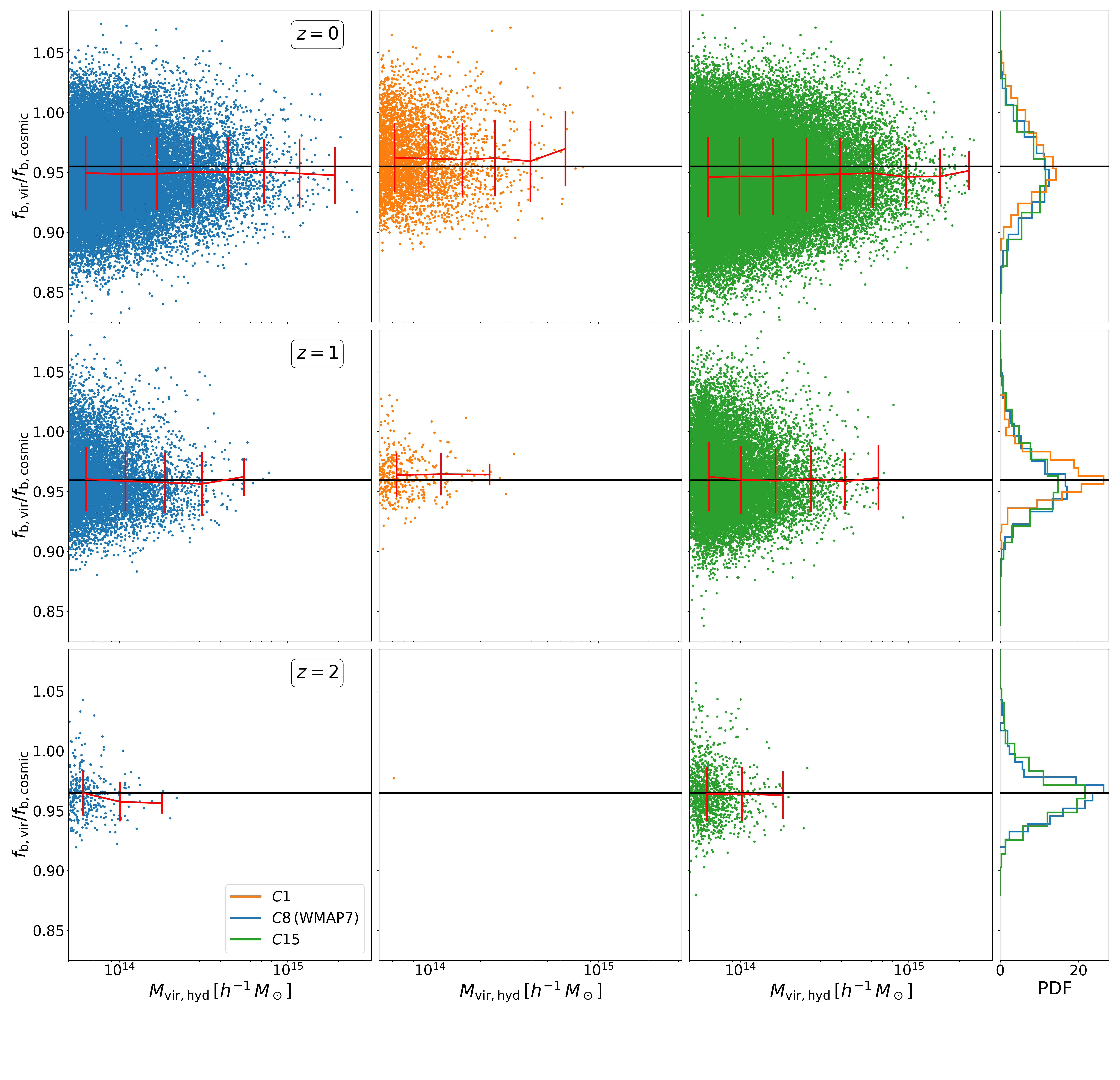
Figure 1: The ratio of baryonic fraction inside the virial radius with respect to the cosmic baryon fraction as a function of the virial mass for the three Magneticum adiabatic runs $C8$, $C1$, and $C15$ depicted in the three columns. Different rows correspond to the redshifts $z\in\{0.0,1.0,2.0\}$. The mean relation, as given by Eq. (14) as a function of redshift, is depicted as the horizontal black line while the red lines correspond to the measured mean and unbiased standard deviations in mass bins. The rightmost column shows the distribution of these ratios, for the three simulations.

3.1.1 Baryonic content in non-radiative simulations

In Fig. 1, we present the ratio between the baryonic fraction inside the virial radius and the cosmic baryon fraction, as a function of the virial mass for the three Magneticum simulations for which the non-radiative version is available: $C8$, $C1$, and $C15$ reported in the three columns. The result for the redshifts $z\in\{0.0,1.0,2.0\}$ is presented in the different rows. The red lines correspond to the mass bins’ measured mean and unbiased standard deviations. We note that the mean baryonic content inside the virial radius scatters around the following relation despite the background cosmological parameters (marked by the horizontal black line):

$$\left\langle\frac{f_{\rm b,vir}}{f_{\rm b,cosmic}}\right\rangle=1-\left(0.045-0.005\,z\right)\,.$$ (14)

The above relation was obtained by fitting a linear relation for the mean relation as a function of redshift.

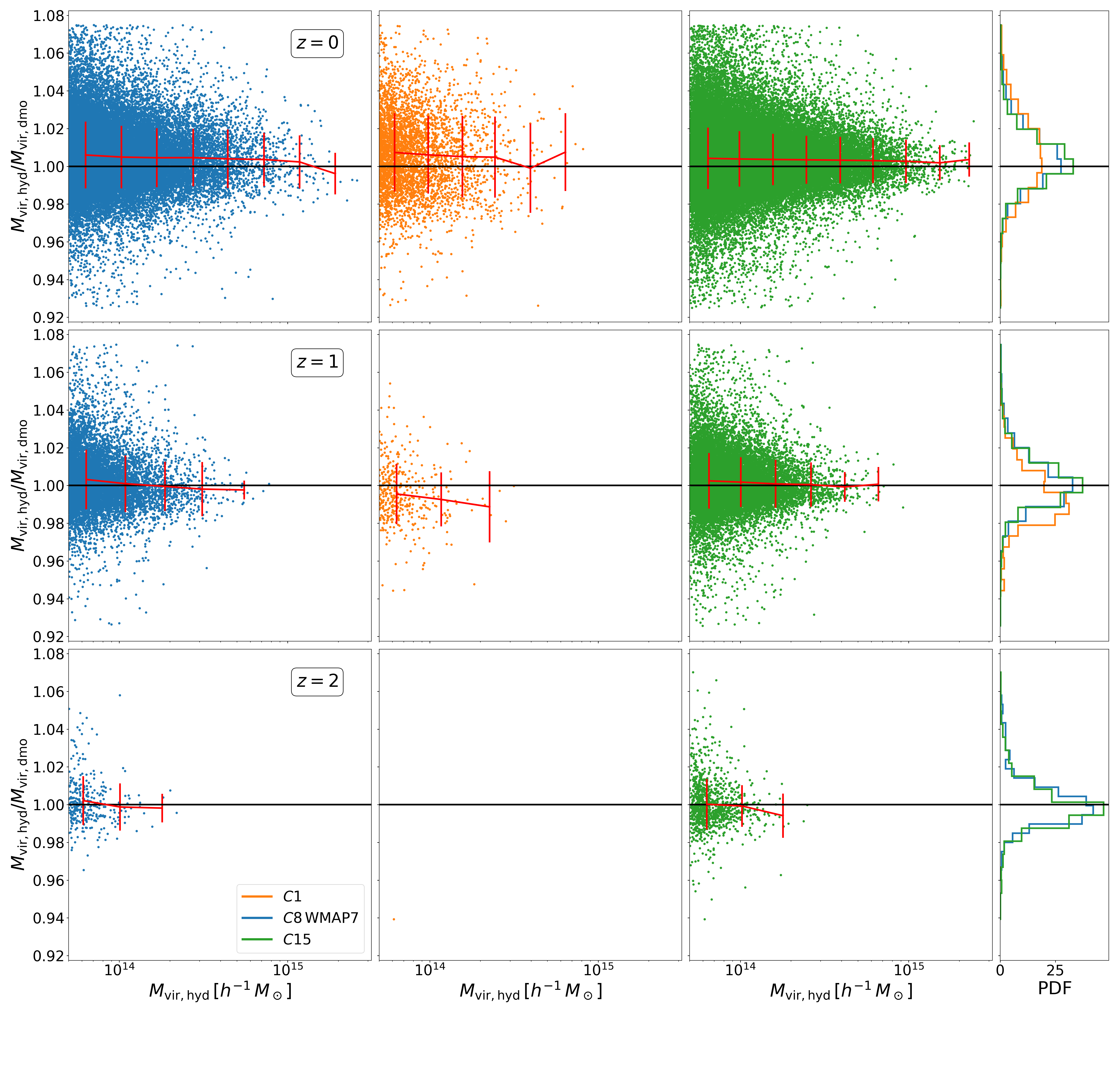
Figure 2: The ratio of the virial mass in the non-radiative run with respect to the matched dmo counterpart for the three Magneticum non-radiative runs. Different rows correspond to the redshifts $z\in\{0.0,1.0,2.0\}$. The unity relation is depicted as the horizontal black line while the red lines correspond to the measured mean and unbiased standard deviations in mass bins.

Conversely, in Fig. 2, we present the ratio of the virial mass in the non-radiative run with respect to the matched dmo counterpart. Despite the missing baryonic content shown in Fig. 1, we observe that halos in the dmo and in the non-radiative simulations have on average the same mass. This leads to the following relation for $\delta_{f}$ in Eqs. (5) and (6):

$$\delta_{f}=(0.045-0.005\,z)\,f_{\rm b,cosmic}\,.$$ (15)

3.1.2 Quasi-adiabatic response

In order to determine the value of the quasi-adiabatic parameter $q$, appearing in Eq. (6) for the model presented in Sect. 2, we proceed in the following way. We bin the halo catalogs of Box $2$ of the Magneticum set at five redshifts, $z\in\{0.00,0.25,0.50,1.00,2.00\}$ in $\log_{10}M_{\rm vir,hyd}/(h^{-1}\,M_{\odot})$ with a bin width of $0.3$ dex. Within each mass bin, we compute the mean and the unbiased standard deviation of the ratio of the virial mass in the hydrodynamic and in the dmo simulations, along with the mean of the ratio of the inferred mass and the true dmo mass. Then, the $\chi^{2}$ between the quasi-adiabatic model and the results from simulations is computed as

$$\chi^{2}=\sum_{i,j}\left(\frac{\langle M_{\rm vir,rec}/M_{\rm vir,dmo}\rangle-\langle M_{\rm vir,hyd}/M_{\rm vir,dmo}\rangle}{\sigma_{i,j}}\right)_{i,j}^{2}\,,$$ (16)

where $i$ and $j$ run over all mass bins and redshifts. In the above equation, $\sigma_{i,j}$ is the error in the binned statistics given by

$$\sigma_{i,j}=\sqrt{\frac{{{\rm{var}}\left(\frac{M_{\rm vir,hyd}}{M_{\rm vir,dmo}}\right)}_{i,j}}{N_{i,j}}+0.003^{2}}\,,$$ (17)

where ${\rm var}$ is the unbiased variance estimation of the ratio of the virial mass in the hydrodynamic and in the dmo simulations, divided by the number of objects in the bin, summed in quadrature with a constant fixed to $0.003$ in order to obtain a reduced $\chi^{2}$ of order of the unity.

In Fig. 3, we plot the values of the $\Delta\chi^{2}$ as a function of $q$, both for single redshifts and for the analysis based on combining all redshifts. We observe that all redshifts prefer significant deviations from the adiabatic prediction ($q=1$). All redshifts present a minimum around the joint analysis minimum $q=0.373$ (presented as the vertical black dotted line). Exceptions occur at $z=0.25$ and $z=2.0$ that have their best-fit shifted to $q\simeq 0.23$ and $q\simeq 0.30$, respectively. Still, assuming Gaussianity, those shifts correspond to only a $2\sigma$ deviation for $z=0.25$ and less than $1\sigma$ for $z=2.0$. Therefore, in the following we will assume the joint analysis best-fit for $q$ to hold at all redshifts.

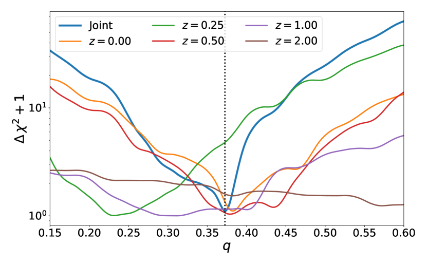
Figure 3: The variation of the $\chi^{2}$ with respect to its minimum, as a function of the quasi-adiabatic parameter $q$ for the model presented in Sect. 2. We present the results for the joint analysis of 5 redshifts $z\in\{0.00,0.25,0.50,1.00,2.00\}$ from the Magneticum Box $2$ simulation, as well as the results at each redshift. The best-fit for $q=0.373$ is marked with the vertical dashed line.

3.2 Validation of the model

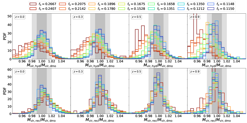
Figure 4: The ratio between either the hydrodynamic mass (top panels) or the reconstructed virial mass (bottom panels) and the dmo counterpart on the sub-set of Magneticum Boxes 1a for the simulations with different cosmologies (see Table 2). Different columns correspond to the $4$ redshifts $z\in\{0.0,0.3,0.5,0.9\}$ and different colors correspond to different cosmic baryon fractions $f_{\rm b}$. The filled dark-grey and light-gray areas mark the $1$ and $2$ percent halo mass variation induced by baryonic effects, respectively.

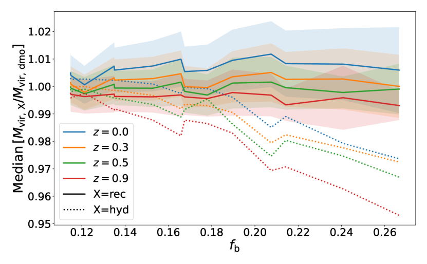
Figure 5: The median of the distributions shown in Fig. 4 as a function of the cosmic baryon fraction $f_{\rm b}$ for the ratio between either the hydrodynamic mass (dotted lines) or the reconstructed virial mass (full lines) and the dmo counterpart on the sub-set of Magneticum Boxes 1a for the simulations with different cosmologies (see Table 2). Different colours correspond to the $4$ redshifts $z\in\{0.0,0.3,0.5,0.9\}$. The filled regions corresponds to one median absolute deviation around the median.

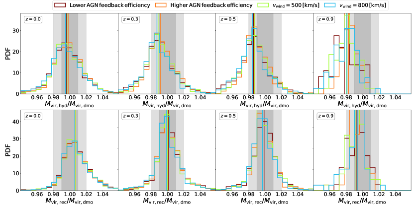
Figure 6: Similar to Fig. 4 but for the simulations with $C8$ (WMAP7) background cosmology that assume different values of the parameters describing SN and AGN feedback.

In Fig. 4, we present the ratio between either the original halo masses in hydro simulations (top panel) or the reconstructed halo masses (bottom panel), and the dmo counterpart. Results are shown for the sub-set of Magneticum Boxes 1a that assume different cosmological parameters (see Table 2), at four redshifts, $z\in\{0.0,0.3,0.5,0.9\}$. The median of the corresponding distributions are shown in Fig. 5. The bottom panel presents the model’s performance in recovering the dmo mass for the simulations with different cosmologies color-coded by the baryon fraction.

As expected, the median value of the ratio between hydro and dmo halo masses shows significant deviations from unity, in a way that becomes more significant as the value of the baryon fraction increases. On the other hand, we see from the bottom panels that our model allows us to correctly recover, on average, the halo masses from the dmo simulations. Quite remarkably, this accuracy is independent of the cosmological model adopted in the simulations, as the correlation of the net effect with the baryonic fraction is absent in the reconstructed mass. In general, dmo masses are recovered by our model with sub-percent accuracy. Possible exceptions are represented by the simulations with the largest cosmic baryon fraction at $z=0$, for which our model seems to slightly over-boost the reconstructed mass by roughly $1$ percent. Lastly, we observe that subdominant to the model target accuracy of $1$ percent, there is a correlation between the model performance and the redshift, with the median of the ratio decreasing with increasing ratio; this hints at a feature missing in our model, such as a redshift dependent quasi-adiabatic factor, needed to take into account to push our model accuracy to sub-percent accuracy. This is left for further investigation in future work.

Similarly to Fig. 4, in Fig. 6 we present the performance of the model for the simulations with $C8$ (WMAP7) background cosmology, but assuming different values for the parameters which define the efficiency of feedback from both AGN and SN. Vertical lines denote the median of the corresponding distribution. In particular, we varied (a) the efficiency of the AGN feedback, by changing the value of the BlackholeFeedbackFactor parameter from 0.1 to 0.2 (default value was 0.15), and (b) the value of the velocity of the SN driven galactic outflows in the model by Springel & Hernquist (2003) from 350 ${\rm km\,s}^{-1}$ to 500 ${\rm km\,s}^{-1}$ and 800 ${\rm km\,s}^{-1}$, respectively. In general, we note that the effect of changing the parameters regulating stellar and AGN feedback is relatively small, especially at low redshift. In any case, the accuracy of our model to recover the halo masses in the dmo simulation does not degrade by changing the feedback parameters. The difference between the vertical lines is always smaller for the reconstructed mass than when considering the actual masses from the hydro simulations.

Similarly to Figs. 4 and 6, in Figs. 7 and 8 we present the performance of the model on the Magneticum Box $2$b and on the TNG-300 simulations, respectively. The different columns present the results for $z\in\{0.2,0.5,1.0,2.0\}$ for Magneticum and $z\in\{0.0,0.5,1.0,2.0\}$ for TNG-300. We note that considering Box 2b instead of Box 1a of the Magneticum set allows us to validate the robustness of our method when increasing resolution. At the same time, the analysis of the TNG-300 box allows us to further stress the validity of our model at a even higher resolution and for a substantially different hydrodynamical solver, star-formation model and implementation of both stellar and AGN feedback. We present the results for two mass regimes: $3\times 10^{13}\leq M_{\rm vir,dmo}/(h^{-1}M_{\odot})<10^{14}$ and $M_{\rm vir,dmo}/(h^{-1}M_{\odot})\geq 10^{14}$. We refer to the former as the group regime and the latter as the regime of galaxy clusters. Note that, due to the smaller size of the TNG-300 box, this simulation does not contain cluster-sized halos at $z=2$. Both simulations predict a stronger impact on the group regime than in the cluster regime; this is expected as on the group regime, the potential well is shallower than in the cluster regime; therefore, the baryonic depletion requires less feedback. In general, TNG-300 predicts a smaller impact of baryonic effects on halo masses in the cluster regime than the Magneticum Box 2b simulation. In any case, our model performs equally well in both simulations and mass regimes. The smaller impact predicted by the TNG-300 simulations is due to the fact that Magneticum and TNG-300 simulations predict a similar baryonic content for virial halos at $z=1$ as can be seen in Fig. 10. However, the cosmic baryon fraction assumed in the Magneticum reference simulation is $\sim 7$ percent higher. Therefore, a stronger gas depletion and more active feedback must occur on Magneticum than on TNG, with a subsequent larger effect on the halo mass associated with a more pronounced gas displacement.

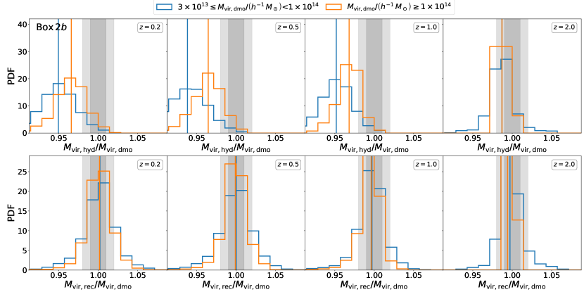
Figure 7: The ratio between either the hydrodynamic mass (top panels) or the reconstructed virial mass (bottom panels), and the dmo counterpart on the Magneticum Boxes 2b. The different columns present the results for $z\in\{0.2,0.5,1.0,2.0\}$. We show the results for two mass regimes: $3\times 10^{13}\leq M_{\rm vir,dmo}/(h^{-1}M_{\odot})<10^{14}$ (blue histograms) and $M_{\rm vir,dmo}/(h^{-1}M_{\odot})\geq 10^{14}$ (orange histograms).

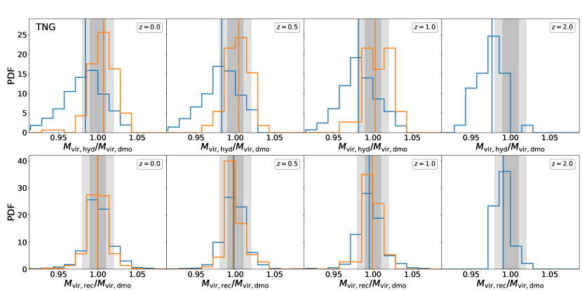
Figure 8: Similar to Fig. 7 but for the TNG-300 simulation.

3.3 Robustness of the model to the assumed baryon fraction relation

In our previous results, we have shown the performance of our model in reconstructing $M_{\rm vir,dmo}$, assuming that the baryon fraction of each halo is known. It is also interesting to understand if one assumes a baryon fraction-mass relation averaged through a sample and uses this instead.

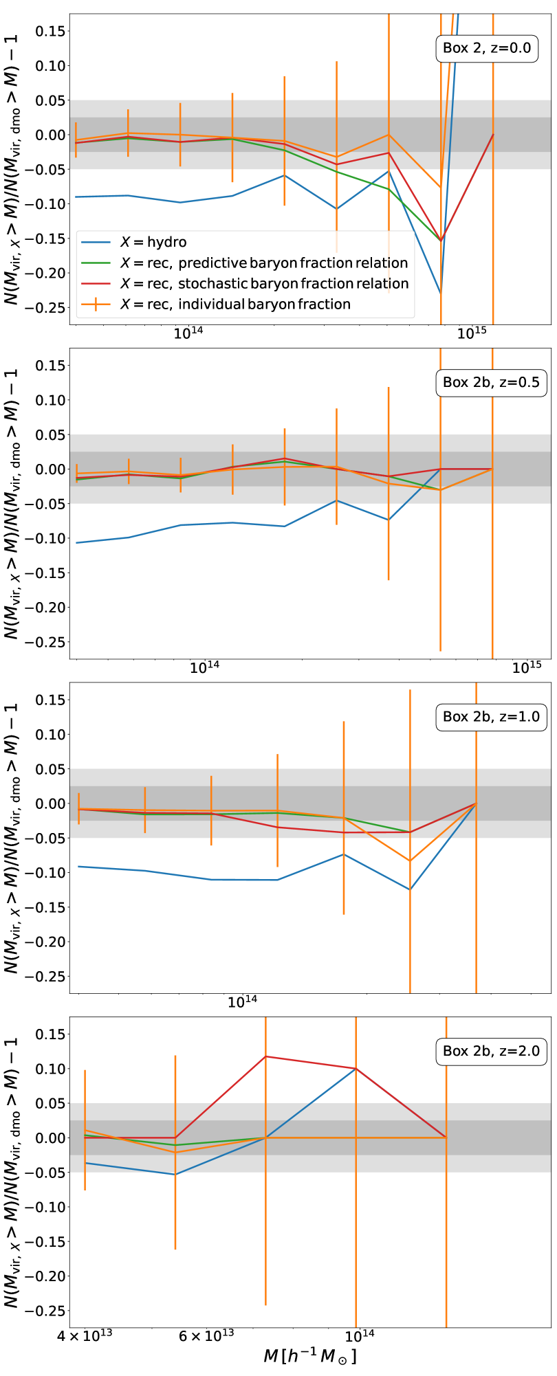
Figure 9: The ratio of the cumulative halo abundance in the hydro simulation to the halo abundance of virial halos in the dmo simulation. The results are shown for the simulated virial mass and the prediction of our model based on the individual baryon fractions as well as a predictive baryon fraction relation. Error bars are displayed for the latter case, assuming uncorrelated Poisson errors. Different panels correspond to redshifts $z\in\{0.0,0.5,1.0,2.0\}$, using Magneticum Box 2b, except for $z=0.0$, where Box 2 is used. The gray regions correspond to $2.5$ and $5$ percent.

In Fig. 9, we present the ratio of the cumulative halo abundance assuming different masses on the hydro simulation with respect to the halo abundance of virial halos on the dmo simulation. We present the results for the virial mass of the hydro simulation as well as the virial prediction of our model if:

1. We assume that the baryon fraction of individual objects is known.

2. We assume a predictive baryon fraction relation given by Eq. (19) with parameters shown in Table 4 for the Magneticum set.

3. We assume a stochastic baryon fraction with mean given by Eq. (19) with parameters shown in Table 4 for the Magneticum set and with a scatter of 0.17 dex.

The third case addresses the possibility that the scatter of the cluster gas fraction in simulation is underestimated compared to observational data. We assume the scatter of $0.17$ dex reported by Andreon et al. (2017) for the gas fraction. For better plot readability, we present error bars only for the second case, assuming uncorrelated Poisson errors for the abundances. Different panels correspond to the redshifts $z\in\{0.0,0.5,1.0,2.0\}$ and for all panels, we use Magneticum Box 2b, but for $z=0.0$ where we use Box 2 as the Box 2b was not run down to this redshift.

In Fig. 9, the baryonic physics tends to produce less massive halos than their dmo counterparts, as previously discussed by Castro et al. (2020). Thus, at fixed mass value, the abundance of halos in a hydro simulation is lower than that derived from a dmo simulation (blue lines). Conversely, converting $M_{\rm vir,hyd}$ to the corresponding dmo virial masses, the abundances of the two simulations match (green and orange lines). Regarding the performance of our model, we note that using a collective relation (red and orange lines) instead of the individual object baryon fraction (green line) does not significantly degrade the mass reconstruction. This is neither obvious nor expected a priori, as non-linear functions do not commute with the median operation. The robustness of the performance comes from the tightness of the baryon fraction relation at fixed mass (see Fig. 10), and ensures the goodness of our model for cluster cosmology applications even if we assume a larger variance for the baryon fraction distribution. Therefore, the approximations that lead to the simplification of Eq. (7) to Eq. (8) are validated and do not statistically affect the model’s performance.

4 Impact of baryonic effects on a Euclid-like cluster abundance analysis

In this section, we quantify the biases in the derivation of the posteriors on the cosmological parameters $\Omega_{\rm m}$ and $\sigma_{8}$, induced by neglecting the baryonic effects on halo masses. In particular, we will quantify such biases by either assuming a fully predictive baryon fraction relation measured on the Magneticum or the TNG-300 simulations when creating the synthetic catalog (see more details on Appendix A). Then, we will assess the capability of our method for recovering halo masses in dmo simulations.

We perform the forecast following the methodology described in Sect. 2.4. For the likelihood analysis, we assume flat priors on the cosmological parameters and Gaussian priors on the mass-observable parameters of Eqs. (10) and (11) with mean given by the fiducial values and with r.m.s. of 1 and 3 percent. The likelihood sampling is performed following the Ensemble Slice Sampling method (see Karamanis & Beutler 2021) implemented in ZEUS (see Karamanis et al. 2021).

Firstly, we assess the tension between the inferred cosmological parameters and the fiducial ones after marginalizing over the other parameters, as quantified by the index of inconsistency (IOI; Lin & Ishak 2017), which is calculated as

$${\rm IOI}=\frac{\boldsymbol{\delta}^{\rm t}\,\boldsymbol{\Sigma}^{-1}\,\boldsymbol{\delta}}{2}\,.$$ (18)

In the above expression, $\boldsymbol{\delta}$ is the two-dimensional difference vector between the best-fit values and the fiducial values of the $\Omega_{\rm m}$ and $\sigma_{8}$ cosmological parameters, while $\boldsymbol{\Sigma}$ is the covariance matrix between these parameters, which we assume to be Gaussian distributed. We calculate the IOI when ignoring the baryonic impact, assuming the cosmological parameters and the virial baryon content relation from the TNG and the Magneticum simulations.

In Table 3, we present the summary statistics for the forecast of the impact of the treatment of the baryonic effects on halo masses for the constraints on $\Omega_{\rm m}$ and $\sigma_{8}$ to be obtained from the cluster counts analysis of the forthcoming Euclid survey. Ideally, the IOI should be kept below 1 to ensure that any correlations with other systematic effects do not amplify tensions in the final results (Euclid Collaboration: Deshpande et al. 2023).

For both Magneticum and TNG simulations, we observe an increasing impact of the baryonic effects on halo masses as stronger priors on the mass-observable scaling relation are assumed. This is an expected result, as a tighter prior on the scaling relation results in tighter constraints on the cosmological parameters, making cosmological posteriors more sensitive to systematic effects. While ignoring baryonic effects in the Magneticum simulations would lead to an IOI of $4.1$ and $2.0$ for $1$ and $3$ percent priors, for TNG-300 these values reduce to $1.8$ and $0.9$, respectively. The reason for the smaller impact of baryons predicted by TNG with respect to Magneticum is two-fold. As discussed in Sect. 3.2, the baryon content observed in massive clusters in TNG-300 is closer to the cosmic baryon fraction assumed in this simulation, thus implying a smaller baryon depletion from the feedback model. Secondly, while in the Magneticum case the recovered posteriors are centered on the fiducial parameters of the scaling relation, for the TNG case we obtained a shift towards lower values of $\sim 1\sigma$ for both cases in the obtained posteriors for $C_{\lambda}$ (the parameter controlling the evolution with redshift). Therefore, the scaling relation degrees of freedom absorb part of the baryonic impact. The absorption of the impact by $C_{\lambda}$ could be anticipated as it is the only parameter in our mass-observation relation that depends on the background evolution as the baryon fraction also does. The redshift dependency of the baryon fraction as a function of mass for the TNG-300 is reported in Table 4.

Note that, in Bocquet et al. (2019) cluster cosmology analysis from the SPT-SZ Survey, $C_{\lambda}$ is especially degenerate with dark energy equation of state parameter $w$ – that we have not considered as a cosmological parameter for our forecast. The absorption of the baryonic impact on $C_{\lambda}$ might likely cause biased dark energy constraints in this case.

In Table 3, we also report the degradation in the constraints on cosmological parameters once we also marginalize over the limited knowledge of the baryon content and the model accuracy, which is described by the $\alpha$ and $\beta$ parameters (see Eqs. 12 and 13). We present the relative change in the figure of merit (FOM; see Huterer & Turner 2001; Albrecht et al. 2006) in the $(\Omega_{\rm m},\sigma_{8})$ plane for different scenarios concerning a hypothetical perfect knowledge of the baryonic content and a perfect performance of the baryonic correction model. Again, we consider $1$ and $3$ percent priors on the richness-mass scaling relations. In all cases, we assume a Gaussian prior on $\beta$ with zero mean and $0.01$ standard deviation in agreement with the accuracy and precision of our model. Concerning the priors on $\alpha$, we consider three scenarios: $0$ (perfect knowledge), $1$ percent, and $10$ percent. For contextualizing, Chiu et al. (2018) claim that the characteristic baryon mass fraction inside $R_{500{\rm c}}$ is about ($12.8\pm 1.3$) percent for clusters with mass $M_{500{\rm c}}=4.8\times 10^{14}\,M_{\odot}$ and at redshift $z=0.6$ based on their analysis of a set of $91$ galaxy clusters from the $2500$ deg² South Pole Telescope SPT-SZ survey (Bleem et al. 2015). Therefore, our $10$ percent priors is in line with the current level of precision in the observational calibration of this relation. For $1$ and $3$ percent priors in the scaling relation and perfect knowledge of the baryon fraction relation, we observe that marginalizing over the accuracy of our model impacts the FOM in the cosmological constraints by $15$ and $11$ percent, respectively. While $1$ percent prior in the baryon fraction relation does not significantly further degrade the FOM for the case where the richness-mass relation is known at $3$ percent, it reduces the FOM by a further $7$ percent if the richness-mass relation is known with $1$ percent precision. Lastly, for $10$ percent prior in the baryon fraction relation, the impact in the FOM is roughly $70$ and $40$ percent for the cases where the richness-mass relation is known at $1$ and $3$ percent precision level.

For all cases considered for the forecast, the correlation between $\alpha$ and $\beta$ and the cosmological parameters is less significant than the correlation between the cosmological parameters themselves. Although the absence of strong correlations between cosmological parameters and $\alpha$ and $\beta$ is a desired feature to improve the analysis robustness, in the specific case of $\alpha$, it was also due to the simplified functional form considered for the uncertainty on the baryon fraction relation. A more detailed analysis of the impact of the baryon fraction relation, considering a more flexible parametrization, is out of the scope of this paper and is left for further investigation.

In summary, the results presented in this section confirm that neglecting baryonic effects on halo masses leads to significantly biased constraints on cosmological parameters from the cluster number counts, especially when strong priors on the mass-observable relation are assumed. On the other hand, we also demonstrate that our model to correct for such baryonic effects allows us to reduce this bias significantly.

Table 3: Summary statistics for the forecast of the impact of baryon mass correction model on Euclid’s cluster counts cosmological constraints on $\Omega_{\rm m}$ and $\sigma_{8}$. The index of inconsistency (IOI) quantifies the tension in the posteriors for the different treatments with respect to a hypothetical perfect knowledge of the model used to create the synthetic data (see text). The figure of merit (FOM) ratio assesses the attenuation of cluster counts’ constraining power once one marginalizes the model’s uncertainties and clusters’ baryon content. For both statistics, errors were estimated by sampling multivariate Gaussian distributions with the correlation extracted from the respective MCMC chains and recomputing the statistics from them.

			$\langle f_{\rm b,vir}(M,z)\rangle$
Summary statistics	richness-mass relation priors	baryonic treatment	relation	prior on $\alpha$	value
IOI	$1\,\%$	ignoring	TNG-300	–	$\hphantom{-}1.8\pm 0.1$
			Magneticum		$\hphantom{-}4.1\pm 0.2$
	$3\,\%$	ignoring	TNG-300	–	$\hphantom{-}0.9\pm 0.1$
			Magneticum		$\hphantom{-}2.0\pm 0.2$
$\frac{\mathrm{FOM}_{\mathrm{corrected}}}{\mathrm{FOM}}$	$1\,\%$	our model	Magneticum	perfect knowledge	$\hphantom{-}0.85\pm 0.02$
				$1\,\%$	$\hphantom{-}0.78\pm 0.02$
				$10\,\%$	$\hphantom{-}0.33\pm 0.01$
	$3\,\%$	our model	Magneticum	perfect knowledge	$\hphantom{-}0.89\pm 0.03$
				$1\,\%$	$\hphantom{-}0.90\pm 0.03$
				$10\,\%$	$\hphantom{-}0.61\pm 0.02$

5 Conclusions

In this paper, we present a model for the impact of baryonic feedback on the virial masses of galaxy clusters. The main aim of our analysis is to verify whether such baryonic effects on halo masses can be modeled with good enough precision so that they do not represent a limiting factor in the cosmological constraining power of the survey of galaxy clusters to be obtained from the Euclid wide photometric survey.

Our model assumes that the feedback effects on the intra-cluster gas follow a quasi-adiabatic behavior and have the baryon fraction inside the virial radius as input. In this case, this effect can be reliably described by a phenomenological model which depends only on $2$ free parameters, to be calibrated against cosmological hydro simulations. Such two parameters control the minimum baryonic depletion observed in non-radiative simulations and the deviation from the adiabatic behavior. Although our model was calibrated using a set of non-radiative hydrodynamic simulations and a single realization of a full-physics simulation, we demonstrated that its performance is resilient to changes in the sub-resolution physics and cosmological parameters. This result is established by confronting our model with different simulations from the Magneticum suite and the TNG-300 simulation. Finally, with the resulting baryonic correction model, we assess the impact of its accuracy and precision in the cosmological parameters inference from an idealized Euclid cluster number counts experiment.

Our main conclusions can be summarised as follows.

• We have shown that the baryonic feedback effects on the intra-cluster gas can be accurately modeled using a quasi-adiabatic approach with two parameters, controlling the minimum baryonic depletion and the deviation from adiabatic behavior.

• We have successfully calibrated these two parameters against cosmological hydro simulations. This model calibration was conducted using a set of non-radiative hydrodynamic simulations as well as a single full-physics simulation.

• Our model attains one percent relative accuracy in determining the virial dmo equivalent mass of simulated galaxy clusters.

• The robustness of our model has been stressed using different simulations from the Magneticum suite and the TNG-300 simulation. Our findings indicate that the model’s effectiveness does not significantly deviate under changes in sub-resolution physics or cosmological parameters, showing strong consistency between our model predictions and these independent simulations.

• Unlike previous works (Cui et al. 2014; Bocquet et al. 2016; Castro et al. 2020), our model does not rely on a single baryonic physics model or assume the universality of the HMF as a function of cosmology. This flexibility represents a significant advantage over other calibrations for the impact of baryonic feedback on the HMF, which cannot predict outcomes under altered baryonic models and implicitly assumes HMF universality.

• The findings of our research substantiate previous claims about the potential significant impact of baryons, if neglected, on the cosmological constraints derived from the Euclid photometric galaxy cluster number counts.

• Most importantly, the uncertainties linked with our model for correcting baryonic effects on cluster masses are shown to be subdominant to the precision of the expected calibration of the mass-observable relation with Euclid as well as our current understanding of the baryon fraction within galaxy clusters.

Lastly, it is important to note that the model presented in this paper is based on the assumption of quasi-adiabatic action of the AGN feedback. Future work could extend the current framework by investigating its validity concerning other prescriptions for AGN feedback as well as additional non-thermal processes not explored in this suite of simulations.

Appendix A Baryon content of galaxy clusters in full-physics simulations

In this appendix we report the results on the baryon content of galaxy clusters and groups within the halo virial radius, for both the Magneticum and the TNG-300 simulations. The results provided here are used in our analysis for the calibration of the parameters which define our model to correct halo masses for baryonic effects. It goes beyond the scope of this analysis to carry out a comparison with observational data.

In Fig. 10 we show the baryonic fraction inside the virial halos, as a function of the halo virial mass, for the Magneticum (upper panels) and TNG-300 (lower panels) simulations, at four different redshifts $z\in\{0.0,0.5,1.0,2.0\}$. The cosmic baryon fraction assumed by the respective simulations is shown as the horizontal black line. The median baryon fraction in halos is shown by the red line and the best-fit for the relation is shown in green. For the Magneticum results we show with orange and blue symbols the results obtained for Box 2 and for Box 1a, respectively. The first one samples at better resolution the mass range of groups and low-mass clusters, while the larger size of the Box 1a allow us to sample at lower resolution the most massive clusters (see Table 1).

The best-fit relations for the Magneticum and TNG-300 are given by

$$f_{\rm b,fid}(m,z)=f_{\rm b,cosmic}\,m^{-\gamma}\,\left(1+m^{1/\delta}\right)^{\gamma\,\delta}\,,$$ (19)

with $m$ given by

$$m=\log_{10}\,\frac{M_{\rm vir}}{10^{14}\,M_{\odot}\,h^{-1}}\,,$$ (20)

while the specific values for the parameters $\gamma$ and $\delta$ and their redshift dependence are shown in Table 4.

Quite interestingly, the depletion of baryons in the Magneticum simulations is more pronounced than in TNG-300, a difference that increases at low redshift. At $z=0$, a depletion of about 10 percent is observed for Magneticum even for the most massive clusters, while the baryon content in TNG-300 clusters saturates to the cosmic value already for $M_{\rm vir}\simeq 2\times 10^{14}M_{\odot}\,h^{-1}$.

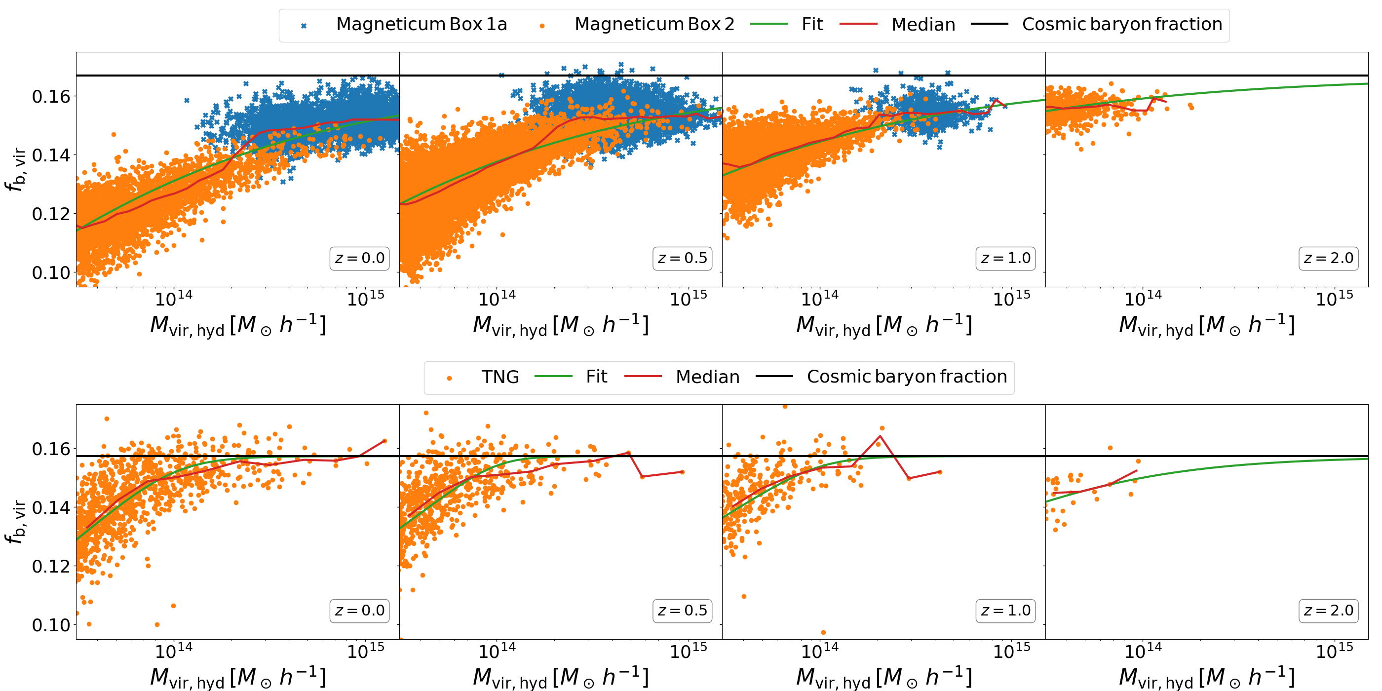
Figure 10: The baryon fraction inside the virial radius as a function of the virial mass. Top: the Magneticum suite of simulations. Orange and blue symbols correspond to Box 2 and Box 1a, respectively. Bottom: the TNG-300 simulation. Different columns correspond to the redshifts $z\in\{0.0,0.5,1.0,2.0\}$. The assumed cosmic baryon fraction for each simulation is depicted as the horizontal black line.

Table 4: Best-fit parameters for the fitting function presented in Eq. (19) for the baryon fraction inside the virial radius for the Magneticum and TNG-300 simulations.

Simulation	$\gamma(z)$	$\delta(z)$
TNG-300	$0.4106\,z-1.4640$	$0.0397\,z^{2}-0.04358\,z+0.03567$
Magneticum	$0.7008\,z-1.7505$	$0.2$