Unstable capillary-gravity waves

Abstract.

We make rigorous spectral stability analysis for non-resonant capillary-gravity waves as well as resonant Wilton ripples of sufficiently small amplitude. Our analysis is based on a periodic Evans function approach, developed recently by the authors for Stokes waves. On top of our previous work, we add to the approach new framework ingredients, including a two-stage Weierstrass preparation manipulation for the Periodic Evans function associated to the wave and the definition of a stability function as an analytic function of the wave amplitude parameter. These new ingredients are keys for proving stability near non-resonant frequencies and defining index functions ruling both stability and instability near non-zero resonant frequencies. We also prove that unstable bubble spectra near non-zero resonant frequencies form, at the leading order, either an ellipse or a circle and provide a justification for Creedon, Deconinck, and Trichtchenko’s formal asymptotic expansion for the Floquet exponent. For non-resonant capillary-gravity waves for the stability near the origin of the complex plane, our stability results agree with the prediction from formal multi-scale expansion. New are our stability results near non-zero resonant frequencies. As the effects of surface tension vanish, our result recovers that for gravity waves. Also new are our stability results for Wilton ripples of small amplitude near the origin as well as near non-zero resonant frequencies.

1. Introduction

We consider capillary-gravity waves (of small amplitude) at the free surface of an incompressible inviscid fluid in two dimensions, under the influence of gravity and surface tension. Suppose for definiteness that in Cartesian coordinates, the wave propagation is in the $x$ direction, and the gravitational acceleration in the negative $y$ direction. Suppose that the fluid at rest occupies the region $\{(x,y)\in\mathbb{R}^{2}:0<y<h\}$, where $h>0$ is the fluid depth. Let

$$y=h+\eta(x,t),\quad x\in\mathbb{R},$$

denote the fluid surface at time $t$, and $y=0$ the rigid bed. Physically realistic is that $h+\eta(x,t)>0$ for all $x\in\mathbb{R}$. Throughout we assume an irrotational flow, whereby a velocity potential $\phi(x,y,t)$ satisfies

$$\phi_{xx}+\phi_{yy}=0 0<y<h+\eta(x,t)$$ for , (1.1a)

subject to the boundary condition

$$\phi_{y}=0 y=0$$ at . (1.1b)

The kinematic and dynamic boundary conditions at the fluid surface are

$$\left.\begin{aligned} &\eta_{t}-c\eta_{x}+\eta_{x}\phi_{x}=\phi_{y}\\ &\phi_{t}-c\phi_{x}+\frac{1}{2}(\phi_{x}^{2}+\phi_{y}^{2})\\ &\quad+g\eta-b\frac{\eta_{xx}}{(1+\eta_{x}^{2})^{3/2}}=q(t)\\ \end{aligned}\right\} \text{at $y=h+\eta(x,t)$},$$ (1.1c)

where $c\neq 0,\in\mathbb{R}$ is the velocity of the wave, $g>0$ the constant of gravitational acceleration, $b\geqslant 0$ is the ratio of the surface tension coefficient to the fluid density, and $q(t)$ is an arbitrary function.

When the effects of surface tension are negligible, that is, $b=0$, (1.1) admits periodic traveling wave solutions, known as the Stokes waves [33] (see also [34]), which are unstable to long wavelength perturbations - namely, the Benjamin-Feir or modulational instability - provided that $\kappa h>1.3627\ldots$ [2, 38] (see also references cited in [40] for others). Here $\kappa$ denotes the wave number of the unperturbed wave. Bridges and Mielke [5] proved rigorously such stability. We pause to mention that, for modulational instability of Stokes waves of infinite depth, see Nguyen and Strauss [27] and Berti, Maspero, and Ventura [3] and, for nonlinear modulational instability of Stokes wave of infinite depth, see recent work of Chen and Su [8]. Additionally, numerical investigations (see, for instance, [21, 22, 25, 12, 10]) revealed that Stokes waves for a wide range of the wavelength and amplitude parameters are spectrally unstable away from the origin of the complex plane when the unperturbed wave is “resonant” with its infinitesimal perturbations. By contrast, the Benjamin–Feir instability refers to the spectrum near the origin. Recently, the authors [17] developed a novel periodic Evans function approach for cylindrical domains, proving that a $2\pi/\kappa$ periodic Stokes wave of sufficiently small amplitude in water of depth $h$ is unstable near the spectrum associated with resonance of order $2$ given an explicitly computable index function [17, $\mathrm{ind}_{2}$(6.34)] is positive. Here we take matters further and make rigorous analysis of spectral stability and instability of capillary-gravity waves, that is, $b>0$, near the origin of the complex plane as well as away from the origin.

Following [17], we reformulate (1.1) in dimensionless variables. Let

$$\begin{gathered}x\mapsto x/h,\qquad y\mapsto y/h,\qquad t\mapsto ct/h,\\ \eta\mapsto\eta/h,\qquad\phi\mapsto\phi/(ch),\qquad q\mapsto q/c^{2},\end{gathered}$$ (1.2)

and let

$$\mu=gh/c^{2}\quad\text{and}\quad\beta=b/(gh^{2})$$ (1.3)

denote the Froude number and the inverse of the Bond number. Substituting (1.2) and (1.3) into (1.1), after some algebra we arrive at

$$\phi_{xx}+\phi_{yy}=0 0<y<1+\eta(x,t)$$ for , (1.4)

$$\phi_{y}=0 y=0$$ at ,

$$\left.\begin{aligned} &\eta_{t}-\eta_{x}+\eta_{x}\phi_{x}=\phi_{y}\\ &\phi_{t}-\phi_{x}+\frac{1}{2}(\phi_{x}^{2}+\phi_{y}^{2})\\ &\quad+\mu\eta-\frac{\beta\mu\eta_{xx}}{(1+\eta_{x}^{2})^{3/2}}=q(t)\end{aligned}\right\} y=1+\eta(x,t)$$ at .

Following [16] (see also [17]), we introduce

$$u=\phi_{x}\quad\text{and}\quad z=\frac{\beta\eta_{x}}{(1+\eta_{x}^{2})^{1/2}}.$$ (1.5)

and make change of variables

$$y\mapsto\frac{y}{1+\eta(x,t)},$$

to reformulate (LABEL:eqn:ww;1) as first order ODEs with respect to the $x$ variable in the infinite cylindrical domain $\mathbb{R}\times(0,1)$. The result becomes

$$\left.\begin{aligned} &\phi_{x}-\frac{yz\phi_{y}}{(1+\eta)\sqrt{\beta^{2}-z^{2}}}-u=0\\ &u_{x}-\frac{yzu_{y}}{(1+\eta)\sqrt{\beta^{2}-z^{2}}}+\frac{\phi_{yy}}{(1+\eta)^{2}}=0\end{aligned}\right\} 0<y<1$$ for , (1.6)

$$\left.\begin{aligned} &\eta_{x}-\frac{z}{\sqrt{\beta^{2}-z^{2}}}=0\\ &\phi_{t}-\mu z_{x}-u+\frac{u^{2}}{2}+\mu\eta\\ &\quad+\frac{(u-1)z\phi_{y}}{(1+\eta)\sqrt{\beta^{2}-z^{2}}}-\frac{\phi_{y}^{2}}{2(1+\eta)^{2}}=q(t)\end{aligned}\right\} \text{at $y=1$},$$

and

$$\phi_{y}=0 \text{at $y=0$},$$ (1.7)

$$\eta_{t}+\frac{z(u-1)}{\sqrt{\beta^{2}-z^{2}}}-\frac{\phi_{y}}{1+\eta}=0\quad \text{at $y=1$}.$$

The third equation of (LABEL:eqn:ww) is obtained through solving the second equation of (1.5), which, for any $\beta\neq 0$, is well defined for sufficiently small amplitude.

In Section 2, we compute the asymptotic expansions for the periodic wave solution known as the capillary-gravity waves and Wilton ripples of order $M\geqslant 2$ occurring when the $\mathcal{O}(\varepsilon^{M})$ terms in the expansion of capillary-gravity waves become singular. Here, $\varepsilon$ is a parameter for the amplitude of the wave. In Section 3, we formulate the spectral problem associated with (LABEL:eqn:ww) and (LABEL:eqn:bd) in abstract form (3.10) $\mathbf{u}_{x}=\mathbf{L}(\lambda)\mathbf{u}+\mathbf{B}(x;\lambda,\varepsilon)\mathbf{u}=:\mathcal{L}(\varepsilon)$ where $\mathbf{L}(\lambda)$ is the leading $\mathcal{O}(1)$ term of $\mathcal{L}(\varepsilon)$ and $\mathbf{B}(x;\lambda,\varepsilon)\mathbf{u}$ is the higher $\mathcal{O}(\varepsilon)$ term. We then make a discussion on the spectrum of $\mathcal{L}(0)$, apply the reduction method by Mielke [26] to reduce the abstract spectral problem to finite dimensions, and hence define an associated periodic Evans function. In Section 3.5 and section 3.6, we illustrate how computations are carried out for the projection to finite dimensions, asymptotic expansions of the reduction function, and the monodromy matrix, which is the most cumbersome part of our analysis and is dealt by using the Matlab math symbolic toolbox. It is impossible to list all of our computations in the write-up. However, we collect some key results in Appendix. We shall also remark that the general framework introduced in Section 3 is applicable to the stability analysis of Wilton ripples of order $M$ when the expansions for capillary-gravity waves become singular.

Main results. Our previous work [17], along with other literature [24, 12, 10], suggests that spectral instability can only occur near resonant frequencies where two purely imaginary eigenvalues of $\mathbf{L}(i\sigma)$ differ by $iN\kappa$. Here, $\sigma\in\mathbb{R}$, $N\in\mathbb{Z}$ and $\kappa$ is the wave number. In Section 4, we establish proofs for these facts by the symmetry of roots (4.5) of the Weierstrass polynomial (4.4) obtained after a first Weierstrass preparation manipulation. See Lemma 4.2, Theorems 4.4 and  4.5, and Remark 1. We note these theories are new, compared to our previous work [17]. We thereby make a discussion for domains of resonant frequencies in the rest of Section 4. In contrast to the zero surface tension case [17], there are capillary-gravity waves admitting resonant frequencies with $N=1$, while Stokes waves can only admit resonant frequencies with $N\geq 2$. Also in contrast to the zero surface tension case, in the case of $\beta>0$, the critical frequencies $-i\sigma_{c,1}$ and $i\sigma_{c,2}$ (see Figures 3 4) can be resonant frequencies that admit two pairs of resonant eigenvalues, making a generalized eigenvector of $\mathbf{L}(\lambda)$ present in the basis of the reduced space at the critical frequencies. See Section 4.2 cases (16)-(19) for details.

In Sections 5.1 and 6.1, at non-zero resonant frequencies, for both non-resonant capillary-gravity waves and Wilton ripples of order $M\geqslant 2$, the Weierstrass polynomials (4.4) obtained after the first Weierstrass preparation manipulation are quadratic. See for instance (5.3), (5.29). In Sections 5.2 and  6.2, at the zero resonant frequency, for non-resonant capillary-gravity waves and for Wilton-ripples of order $M\geqslant 2$, the Weierstrass polynomial is quartic and sextic, respectively. See (5.49) and (6.37).

In the foregoing case of non-zero resonant frequencies where the corresponding Weierstrass polynomials are quadratic, thanks to the simplicity of quadratic formula, our later analysis for their roots is rigorous. Indeed, the symmetry of roots (4.5) of the Weierstrass polynomial (4.4) forces that (4.6) holds for its coefficients. Using (4.6) for the quadratic Weierstrass polynomial (5.3), we make a critical observation in Corollary 5.2 that spectral stability near the resonant frequency is completely determined by the sign of its real-valued discriminant ${\rm disc}(\gamma,\varepsilon)$ (5.5) and is independent of the linear term of (5.3). To determine the sign of ${\rm disc}(\gamma,\varepsilon)$ for fixed $|\varepsilon|\ll 1$ and varied $|\gamma|\ll 1$, its analyticity at $(0,0)$ suggests a second Weierstrass preparation manipulation, resulting always in a quadratic Weierstrass polynomial $W(\gamma,\varepsilon)$ (5.8) in $\gamma$. Lemma 5.3 implies that the sign of ${\rm disc}(\gamma,\varepsilon)$ is opposite to that of $W(\gamma,\varepsilon)$, motivating Definition 5.4 of the stability function ${\rm disc}_{2}(\varepsilon)$ as the discriminant of $W(\gamma,\varepsilon)$, whose sign, for $|\varepsilon|\ll 1$, rules the stability. Still by Definition 5.4, since ${\rm disc}_{2}(\varepsilon)$ is analytic and vanishing at $\varepsilon=0$, its sign for $|\varepsilon|\ll 1$ is determined via the sign of the coefficient of the lowest non-vanishing term in the power series expansion. This coefficient was referred to as the index function in our previous work [17]. We pause to remark the second Weierstrass preparation manipulation is new, compared to our previous work [17]. In [17, Theorem 6.5], positivity of the index function ${\rm ind}_{2}(\kappa)$ (6.34) implies spectral instability near the resonant frequency, while negativity of ${\rm ind}_{2}(\kappa)$ only restrictively implies spectral stability at the order of $\varepsilon^{2}$ as $\varepsilon\rightarrow 0$, making the statement for stability rather weak. With our new general framework of analysis, we remove the weakness in the latter stability statement and now negativity of ${\rm ind}_{2}(\kappa)$ implies spectral stability near the resonant frequency. We make this clear in Remark 4 and Theorem 5.10. As for the shapes of unstable spectra, we further make Corollaries  5.6, 5.11, 5.18, 5.21, 6.3, 6.7, and  6.11. From which we conclude that (i) the bubble spectra are, at the leading order, either in the shape of an ellipse or a circle, depending on if the resonant frequencies are critical (See Remark 8), and (ii) the centers of the bubbles are not necessarily at the resonant frequencies $i\sigma$ and can drift from $i\sigma$ (see Remarks 5 and  7).

For stability away from the origin, our previous work for Stokes waves [17] only treated non-zero resonant frequencies of order $N=2$ and left $N\geqslant 3$ for future investigation. Based on formal asymptotic expansions of the linear perturbation variables (including the Floquet exponent), Creedon et al. [9] studied the spectrum of Stokes waves near resonant frequencies up to $N=3$. In Section 5.1.3, we attempt to treat at resonant frequencies with $N\geqslant 3$. It turns out, by Lemma 5.13, the newly defined stability function ${\rm disc}_{2}(\varepsilon)$ vanishes at $\mathcal{O}(\varepsilon^{4})$-order, whence stability is determined by the next non-vanishing term, which necessarily requires the computations of $\mathbf{a}^{(m,n)}$ (3.50) for $m+n\geqslant 3$, a matter of tedious symbolic computation. We will not pursue in this direction. In current work, our computation of $\mathbf{a}^{(m,n)}$ is still limited up to $m+n=2$, which is sufficient for determining stability near resonant frequencies listed in TABLE 1. Nonetheless, we make use of the new general framework of analysis to justify Creedon et al.’s formal asymptotic expansion for the Floquet exponent [9, (5.1c)]. See Corollary 5.15. We also conjecture the expansion of the stability function ${\rm disc}_{2}(\varepsilon)$ at the resonant frequency $i\sigma$ with $N\geqslant 1$ in general. See (5.25).

In the latter case of zero resonant frequency, a quartic or sextic polynomial is certainly harder to deal with. Nonetheless, since, over the field of reals, polynomials with real coefficients can be factorized as products of irreducible factors with degrees at most two, the real polynomial $\tilde{W}(\tilde{\delta},\gamma,\varepsilon)$ (4.7) can be factorized into quadratic and linear factors, making the analysis after accessible. Though we do not see, in a moment, how such factorization proposed can be achieved, Berti et al. [3] [4] obtained detailed descriptions for the spectra near the origin. Their proofs involve a series of block-diagonalizations that reduce a $4$ by $4$ matrix to two $2$ by $2$ block matrices, whereby a quadratic form is seen. Algebraically, the process of block-diagonalizations is equivalent to the factorization as we proposed here. Berti et al.’s result [4, Theorem 1.1] further implies that, for Stokes waves of finite depth, the potentially unstable roots of the quartic polynomial follow an asymptotic expansion [17, (5.27)]. For non-resonant capillary-gravity waves, we expect the same asymptotic expansion (5.51) shall hold and use it to derive index functions (5.58) (E.2), which gives the same stability diagram as Djordjevic and Redekopp’s [11]. For resonant Wilton ripples, Trichtchenko, Deconinck, and Wilkening [36] numerically computed the unstable spectra near the origin for some choices of wave parameters. It will be very interesting to apply Berti et al.’s methods to understand fully the modulational (in)stability of Wilton ripples. Without further justification, we interpret our results in Sections 5.2 and  6.2 as formal ones. Nonetheless, we emphasize our former rigorous treatment for the non-modulational stability near non-zero resonant frequencies for both non-resonant capillary-gravity waves and resonant Wilton ripples. To our knowledge, the only other contribution aiming at rigorous analysis of spectral stability away from the origin is made by Noble, Rodrigues, and Sun [29] for small-amplitude periodic traveling waves of the electronic Euler-Poisson system and by the use of Krein signature.

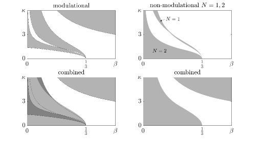
Figure 1. Unstable non-resonant capillary-gravity waves. Top left panel: unstable waves that are subject to modulational instability. These waves achieve unstable spectra near the origin. Note that the modulational stability diagram (see also FIGURE 14) is first obtained by Djordjevic and Redekopp [11]. We mark the boundaries with solid curves. Top right panel: unstable waves that are subject to non-modulational instability. These waves achieve unstable spectra near the resonant frequencies $i\sigma$ with $N=1,2$. We do not mark the boundaries with solid curves. Bottom left panel: unstable waves that are either subject to the modulational instability or non-modulational instability. We note that waves in the dark shaded regions are subject to both modulational and non-modulational instability and the solid curves in light shaded regions separate waves that are only subject to modulational instability from waves that are only subject to non-modulational instability. Bottom right panel: unstable waves that are either subject to the modulational instability or non-modulational instability (with no difference in shading compared to left bottom panel). We note waves in the unshaded region are stable both near the origin and near resonant frequencies with $N=1,2$ and their stability depends on further study at resonant frequencies with $N\geqslant 3$.

We collect all stability results for non-resonant capillary-gravity waves in Section 5 and for Wilton ripples of order $M$ in Section 6. Readers will find the results are quite delicate because of the following facts: (i) non-resonant capillary-gravity waves and Wilton ripples need to be treated separately; (ii) despite that $0$ is a resonant frequency (modulational stability), resonant frequencies $i\sigma$ can also occur at $0<\sigma<\min\{-\sigma_{c,1},\sigma_{c,2}\}$ where the reduced space is six dimensional, at $\min\{-\sigma_{c,1},\sigma_{c,2}\}<\sigma<\max\{-\sigma_{c,1},\sigma_{c,2}\}$ where the reduced space is four dimensional, at $\sigma>\max\{-\sigma_{c,1},\sigma_{c,2}\}$ where the reduced space is two dimensional, and at the critical frequency $-i\sigma_{c,1}$ and $i\sigma_{c,2}$ where there are two pairs of resonant eigenvalues; (iii) the additional terms in the expansion of Wilton ripples of order $M$ complicate wave-wave interactions. The complexities give rise to 12 stability index functions, computable as explicit symbolic expressions of $\kappa,\beta,\sigma$, and resonant eigenvalues $ik_{j}$ of $\mathbf{L}(i\sigma)$. To help readers navigate through these sections, we summarize the stability index functions defined for capillary-gravity waves in Table 1.

wave	resonant frequency $i\sigma$	index	Theorem
non-resonant capillary-gravity	$0<\sigma\neq-\sigma_{c,1},\sigma_{c,2}$, $N=1$	${\rm ind}_{1}$	5.5
	$0<\sigma\neq-\sigma_{c,1},\sigma_{c,2}$, $N=2$	${\rm ind}_{2}$	5.9
	$\sigma=-\sigma_{c,1},\sigma_{c,2}$, $N=1$	${\rm ind}_{3}$	5.17
	$\sigma=-\sigma_{c,1},\sigma_{c,2}$, $N=2$	${\rm ind}_{4}$	5.20
	$0<\sigma$, $N\geqslant 3$	N.A.	N.A.
	$\sigma=0$	${\rm ind}_{5}$	5.25
Wilton ripples of order $2$	$0<\sigma\neq-\sigma_{c,1},\sigma_{c,2}$, $N=2$	${\rm ind}_{6}$	6.2
	$0<\sigma\neq-\sigma_{c,1},\sigma_{c,2}$, $N\geqslant 3$	N.A.	N.A.
	$\sigma=-\sigma_{c,1},\sigma_{c,2}$	N.A.	N.A.
	$\sigma=0$	${\rm ind}_{11,12}$	6.15
Wilton ripples of order $M\geqslant 3$	$0<\sigma\neq-\sigma_{c,1},\sigma_{c,2}$, $N=1$	${\rm ind}_{1}$	6.5
	$0<\sigma\neq-\sigma_{c,1},\sigma_{c,2}$, $N=M$	${\rm ind}_{7}$	6.6
	$0<\sigma\neq-\sigma_{c,1},\sigma_{c,2}$, $N=2,M-1,M+1,2M$	${\rm ind}_{8}$	6.9
	$0<\sigma\neq-\sigma_{c,1},\sigma_{c,2}$, $N\neq 1,2,M-1,M,M+1,2M$	N.A.	N.A.
	$\sigma=-\sigma_{c,1},\sigma_{c,2}$	N.A.	N.A.
	$\sigma=0$	${\rm ind}_{9,10}$	6.13

Table 1. Summary of stability index functions defined for non-resonant capillary-gravity waves and Wilton ripples at a resonant frequency $i\sigma$. In the table, N.A. stands for “Not Available”. See explanation in Section 5.1.3.

We evaluate these index functions by floating-point arithmetic to obtain numerical thresholds for unstable waves, which are listed following the corresponding theorems. Analogous to [17, p. 41 - p. 42], one can upgrade the floating-point arithmetic to interval arithmetic, and thereby rigorously validate the sign of index functions. We will not make the upgrade because of unboundedness of the parameter domains and lack of necessity for the validated numerics. For non-resonant capillary-gravity waves, we collect results obtained from Sections 5.1.4,  5.1.7, and  5.2 and make diagrams 1 showing unstable waves that are either subject to the modulational instability or instability near the resonant frequencies with $N=1,2$, where we refer to the latter instability as non-modulational. In all figures of the paper, we shade the regions where waves are found unstable. For resonant Wilton ripples, we do not make diagrams for the domains of Wilton ripples of order $M$ are one-dimensional curves.

Discussion and open problems. Capillary-gravity waves in the unshaded region of the bottom right panel of FIGURE 1, though are stable both near the origin and near resonant frequencies with $N=1,2$, are not yet proven stable at other (infinitely many) resonant frequencies with $N\geqslant 3$. This is main reason that we emphasize by the title of the work that our results select out unstable waves (particularly in addition to waves that are already found modulationally unstable [11]). Since examining stability at infinite many resonant frequencies is an unrealistic task, it is very interesting to show if one can prove or disprove that a high-frequency stability statement: “there is no unstable spectrum near resonant frequency with $N$ for all $N>N_{*}$, where $N_{*}$ is a sufficiently large integer. The high-stability stability statement once proven will then reduce the examination at finitely many resonant frequencies.

Acknowledgement. The work of VMH was partially supported by NSF through the award DMS-2009981. ZY thanks the Department of Mathematics at the University of Illinois at Urbana-Champaign for the valuable postdoc research and teaching experience.

2. Periodic traveling waves of sufficiently small amplitude

We seek a temporally stationary and spatially periodic solution of (LABEL:eqn:ww)-(LABEL:eqn:bd). That is,

$$\phi,\quad\eta,\quad u=\phi_{x}-\frac{y\eta_{x}\phi_{y}}{1+\eta},\quad\text{and}\quad z=\frac{\beta\eta_{x}}{(1+\eta_{x}^{2})^{1/2}}$$ (2.1a)

satisfy

$$u_{x}-\frac{y\eta_{x}u_{y}}{1+\eta}+\frac{\phi_{yy}}{(1+\eta)^{2}}=0 0<y<1$$ for , (2.1b)

$$\phi_{y}=0 y=0$$ at , (2.1c)

$$(u-1)\eta_{x}-\frac{\phi_{y}}{1+\eta}=0 \text{at $y=1$},$$ (2.1d)

$$\mu z_{x}+u-\frac{u^{2}}{2}-\mu\eta-\frac{\phi_{y}^{2}}{2(1+\eta)^{2}}+q=0 \text{at $y=1$},$$ (2.1e)

where $q$ is a constant, (2.1a) follows from the first and third equations of (LABEL:eqn:ww), and (2.1e) follows from (2.1d) and

$$\mu z_{x}+u-\frac{u^{2}}{2}-\mu\eta-\frac{(u-1)\eta_{x}\phi_{y}}{1+\eta}+\frac{\phi_{y}^{2}}{2(1+\eta)^{2}}+q=0\quad\text{at $y=1$},$$

by the fourth equation of (LABEL:eqn:ww).

We focus the attention on the small amplitude asymptotics. Suppose that

$$\varepsilon\in\mathbb{R}$$ denotes the dimensionless amplitude parameter

and

$$\phi(x,y;\varepsilon)=\phi_{1}(x,y)\varepsilon+\phi_{2}(x,y)\varepsilon^{2}+\phi_{3}(x,y)\varepsilon^{3}+\mathcal{O}(\varepsilon^{4}),$$ (2.2)

$$\eta(x;\varepsilon)=\eta_{1}(x)\varepsilon+\eta_{2}(x)\varepsilon^{2}+\eta_{3}(x)\varepsilon^{3}+\mathcal{O}(\varepsilon^{4}),$$

$$\mu(\varepsilon)=\mu_{0}+\mu_{1}\varepsilon+\mu_{2}\varepsilon^{2}+\mu_{3}\varepsilon^{3}+\mathcal{O}(\varepsilon^{4}),$$

$$q(\varepsilon)=q_{1}\varepsilon+q_{2}\varepsilon^{2}+q_{3}\varepsilon^{3}+\mathcal{O}(\varepsilon^{4}),$$

as $\varepsilon\to 0$, where $\phi_{1},\phi_{2},\phi_{3},\dots$, $\eta_{1},\eta_{2},\eta_{3},\dots$, $\mu_{0},\mu_{1},\mu_{2},\mu_{3},\dots$, $q_{1},q_{2},q_{3},\dots$ are to be determined and, hence,

$$u(x,y;\varepsilon)=u_{1}(x,y)\varepsilon+u_{2}(x,y)\varepsilon^{2}+u_{3}(x,y)\varepsilon^{3}+\mathcal{O}(\varepsilon^{4}),$$

$$z(x;\varepsilon)=z_{1}(x)\varepsilon+z_{2}(x)\varepsilon^{2}+z_{3}(x)\varepsilon^{3}+\mathcal{O}(\varepsilon^{4}),$$

as $\varepsilon\to 0$, where $u_{1},u_{2},u_{3},\dots$ and $z_{1},z_{2},z_{3},\dots$ can be determined in terms of $\phi_{1},\phi_{2},\phi_{3},\dots$ and $\eta_{1},\eta_{2},\eta_{3},\dots$ by (2.1a). We assume that $\phi_{1},\phi_{2},\phi_{3},\dots$ and $\eta_{1},\eta_{2},\eta_{3},\dots$ are $T$ periodic functions of $x$, where

$$T=2\pi/\kappa \kappa>0$$ and is the wave number,

and $\mu_{0},\mu_{1},\mu_{2},\mu_{3},\dots$ and $q_{1},q_{2},q_{3},\dots$ are constants. We may assume that $\phi_{1},\phi_{2},\phi_{3},\dots$ are odd functions of $x$, and $\eta_{1},\eta_{2},\eta_{3},\dots$ are even functions and of mean zero over one period. We remark that (2.2) converges for $\varepsilon\in\mathbb{R}$ and $|\varepsilon|\ll 1$, for instance, in $H^{s+2}(\mathbb{R}/T\mathbb{Z}\times(0,1))\times H^{s+5/2}(\mathbb{R}/T\mathbb{Z})\times\mathbb{R}\times\mathbb{R}$ for any $s>1$ [28]. Therefore $\phi(\varepsilon)$, $\eta(\varepsilon)$, $\mu(\varepsilon)$ and $q(\varepsilon)$ depend real analytically on $\varepsilon$ for $|\varepsilon|\ll 1$.

Notation.  In what follows we employ the notation

$$\,{\rm s}(\cdot) =\sin(\cdot), \,{\rm c}(\cdot) =\cos(\cdot),$$

$$\,{\rm sh}(\cdot) =\sinh(\cdot), \,{\rm ch}(\cdot) =\cosh(\cdot), \,{\rm th}(\cdot) =\tanh(\cdot).$$

2.1. Non-resonant capillary-gravity waves

Substituting (2.2) into (2.1), after some algebra, we gather that at the order of $\varepsilon$,

$${\phi_{1}}_{xx}+{\phi_{1}}_{yy}=0 \text{for $0<y<1$},$$ (2.3)

$${\phi_{1}}_{y}=0 \text{at $y=0$},$$

$${\eta_{1}}_{x}+{\phi_{1}}_{y}=0 \text{at $y=1$},$$

$$\mu_{0}\beta{\eta_{1}}_{xx}+{\phi_{1}}_{x}-\mu_{0}\eta_{1}+q_{1}=0\quad \text{at $y=1$}.$$

Recall that $\phi_{1}$ and $\eta_{1}$ are $2\pi/\kappa$ periodic functions of $x$, where $\kappa>0$, $\phi_{1}$ is an odd function of $x$, $\eta_{1}$ is an even function and of mean zero over the period, and $q_{1}$ and $\mu_{0}$ are constants. We solve (LABEL:eqn:stokes1), for instance, by separation of variables, to obtain

$$\phi_{1}(x,y)=\,{\rm s}(\kappa x)\,{\rm ch}(\kappa y),\qquad\eta_{1}(x)=\,{\rm sh}(\kappa)\,{\rm c}(\kappa x),\qquad q_{1}=0$$ (2.4)

and

$$\mu_{0}(1+\beta\kappa^{2})\,{\rm th}(\kappa)-\kappa=0,$$ (2.5)

whence

$$\mu_{0}(\kappa;\beta)=\frac{\kappa}{(1+\beta\kappa^{2})\,{\rm th}(\kappa)}.$$ (2.6)

We remark that (2.6) or, equivalently,

$$c_{0}^{2}=(g+b\kappa^{2})\frac{\,{\rm th}(\kappa h)}{\kappa}$$

gives the well-known dispersion relation for capillary-gravity waves. Clearly, for any $\beta>0$, $\mu_{0}(0^{+};\beta)=1$ and $\mu_{0}(+\infty;\beta)=0$.

Lemma 2.1.

If $\beta\geqslant 1/3$, $\mu_{0}(\cdot;\beta)$ is strictly decreasing on $(0,\infty)$. On the other hand, if $0<\beta<1/3$, there exists a unique $\kappa_{*}>0$ such that $\frac{d\mu_{0}}{d\kappa}(\kappa_{*};\beta)=0$ and $\mu_{0}(\cdot;\beta)$ is strictly increasing on $(0,\kappa_{*})$ and strictly decreasing on $(\kappa_{*},\infty)$.

Proof.

We compute

$$\frac{d\mu_{0}}{d\kappa}(\kappa;\beta)=-\frac{\kappa^{2}\big{(}\,{\rm th}(\kappa)+\kappa(1-\,{\rm th}(\kappa)^{2})\big{)}(\beta-\beta_{S_{1},S_{2}}(\kappa))}{(\beta\kappa^{2}+1)^{2}\,{\rm th}(\kappa)^{2}},$$

where

$$\beta_{S_{1},S_{2}}(\kappa):=\frac{\,{\rm sh}(2\kappa)-2\kappa}{\kappa^{2}(2\kappa+\,{\rm sh}(2\kappa))}.$$ (2.7)

Because $\,{\rm th}(\kappa)<1$ for $\kappa>0$, the sign of $\frac{d\mu_{0}}{d\kappa}(\kappa;\beta)$ is determined by that of $\beta-\beta_{S_{1},S_{2}}(\kappa)$. Clearly $\beta_{S_{1},S_{2}}(+\infty)=0$ and, by L’Hospital rule, $\beta_{S_{1},S_{2}}(0^{+})=\frac{1}{3}$. We now show $\beta_{S_{1},S_{2}}(\kappa)$ is strictly decreasing on $(0,+\infty)$. Further computation reveals

$$\frac{d\beta_{S_{1},S_{2}}(\kappa)}{d\kappa}=-\frac{2(e^{2\kappa}+1)\#(\kappa)}{\kappa^{3}(e^{4\kappa}+4\kappa e^{2\kappa}-1)^{2}},$$

where

$$\#(\kappa):=e^{6\kappa}+(-8\kappa^{2}+4\kappa-1)e^{4\kappa}+(-8\kappa^{2}-4\kappa-1)e^{2\kappa}+1$$

satisfies

$$\#(0),\frac{d\#}{d\kappa}(0),\frac{d^{2}\#}{d\kappa^{2}}(0),\frac{d^{3}\#}{d\kappa^{3}}(0),\frac{d^{4}\#}{d\kappa^{4}}(0),\frac{d^{5}\#}{d\kappa^{5}}(0)=0,\;\;\text{and}\;\;\frac{d^{6}\#}{d\kappa^{6}}(0)=1024.$$

It follows from the mean value theorem that

$$\#(\kappa)=\kappa^{(1)}\kappa^{(2)}\kappa^{(3)}\kappa^{(4)}\kappa^{(5)}\frac{d^{6}\#}{d\kappa^{6}}(\kappa^{(6)})\kappa\quad\text{for some $\kappa^{(n)}$, $n=1,2,3,4$,}$$

such that $0<\kappa^{(6)}<\kappa^{(5)}<\kappa^{(4)}<\kappa^{(3)}<\kappa^{(2)}<\kappa^{(1)}<\kappa$. An INTLAB computation [32] shows

$$\frac{d^{6}\#(\kappa)}{d\kappa^{6}}(\text{infsup}(0,0.001))=[0.48576425206934,1.56320790772994]\times 10^{3},$$

where $\text{infsup}(0,0.001)$ denotes an interval rigorously enclosing $[0,0.001]$, accounting for rounding error, and the right side rigorously encloses the range of $\frac{d^{6}\#}{d\kappa^{6}}(\kappa)$ for $\kappa\in[0,0.001]$. This justifies $\frac{d^{6}\#}{d\kappa^{6}}(\kappa)>0$ for $\kappa\in[0,0.001]$ and, hence, $\#(\kappa)>0$ for $\kappa\in(0,0.001]$.

We turn to $\kappa\gg 1$, say, $\kappa\in(2,\infty)$, where there holds

$$\#(\kappa)=(e^{2\kappa}-8\kappa^{2})e^{4\kappa}+((4\kappa-1)e^{2\kappa}-8\kappa^{2}-4\kappa-1)e^{2\kappa}+1>0.$$

It remains to treat $\kappa\in[0.001,2]$. We divide the interval into finitely many subintervals $I_{n}$ and verify by means of validated numerics that $\inf(\#(I_{n}))>0$ for each subinterval. Combining the above, for $\kappa\in(0,\infty)$, $\#(\kappa)>0$, yielding $\frac{d\beta_{S_{1},S_{2}}(\kappa)}{d\kappa}<0$. ∎

The left and middle panels of Figure 2 depict $\mu_{0}(\cdot;\beta)$ (2.6). By Lemma 2.1, it follows that

• When $\beta\geqslant 1/3$ and $0<\mu_{0}<1$, (2.5) holds true for a unique $\kappa>0$;

• When $\beta\geqslant 1/3$ and $\mu_{0}\geqslant 1$, (2.5) does not hold true for any $\kappa>0$;

• When $0<\beta<1/3$ and $0<\mu_{0}\leqslant 1$, (2.5) holds true for a unique $\kappa>0$;

• When $0<\beta<1/3$ and $1<\mu_{0}\leqslant\mu_{0}(\kappa_{*};\beta)$, where $\mu_{0}(\kappa_{*};\beta)$ is the maximum of $\mu_{0}(\cdot;\beta)$, (2.5) holds true for $\kappa_{1}$ and $\kappa_{2}$, such that $0<\kappa_{1}\leqslant\kappa_{*}\leqslant\kappa_{2}$;

• When $0<\beta<1/3$ and $\mu_{0}>\mu_{0}(\kappa_{*};\beta)$, (2.5) does not hold true for any $\kappa>0$.

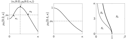
Figure 2. Left panel: The graph of $\mu_{0}(\kappa)$ when $\beta=0.2(<1/3)$. Middle panel: The graph of $\mu_{0}(\kappa)$ when $\beta=0.4(>1/3)$. Right panel: $\kappa$ versus $\beta$ for capillary-gravity waves. The bold curve given by $\beta=\beta_{S_{2},S_{3}}(\kappa)$ (2.8) and along which $\mu_{0}=1$ separates the region of sub-critical waves, for which $\mu_{0}<1$, from the region of super-critical waves, for which $\mu_{0}>1$. The thin curve given by $\beta=\beta_{S_{1},S_{2}}(\kappa)$ (2.7) and along which $\frac{d\mu_{0}}{d\kappa}(\kappa;\beta)=0$ further divides the region of super-critical waves into the regions of $2\pi/\kappa_{1}$ and $2\pi/\kappa_{2}$ periodic waves, where $0<\kappa_{1}\leqslant\kappa_{*}\leqslant\kappa_{2}$.

In the right panel of Figure 2, we distinguish sub-critical waves in the $S_{3}$ region, for which $\mu_{0}<1$, from super-critical waves to the left of a bold curve, given by

$$\beta_{S_{2},S_{3}}(\kappa)=\frac{\kappa-\,{\rm th}(\kappa)}{\kappa^{2}\,{\rm th}(\kappa)},$$ (2.8)

for which $\mu_{0}>1$. Moreover, for super-critical waves, we separate, by a thin curve $\beta=\beta_{S_{1},S_{2}}(\kappa)$, $2\pi/\kappa_{1}$ periodic waves in the $S_{1}$ region and $2\pi/\kappa_{2}$ periodic waves in the $S_{2}$ region, where $0<\kappa_{1}\leqslant\kappa_{*}\leqslant\kappa_{2}$.

To proceed, at the order of $\varepsilon^{2}$, we gather

$${\phi_{2}}_{xx}+{\phi_{2}}_{yy}=2\eta_{1}{\phi_{1}}_{yy}+y{\eta_{1}}_{xx}{\phi_{1}}_{y}+2y{\eta_{1}}_{x}{\phi_{1}}_{xy} \text{for $0<y<1$},$$ (2.9)

$${\phi_{2}}_{y}=0 \text{at $y=0$},$$

$${\eta_{2}}_{x}+{\phi_{2}}_{y}={\eta_{1}}_{x}{\phi_{1}}_{x}+\eta_{1}{\phi_{1}}_{y} \text{at $y=1$},$$

$$\begin{aligned} &\mu_{0}\beta{\eta_{2}}_{xx}+{\phi_{2}}_{x}-\mu_{0}\eta_{2}+q_{2}=-\mu_{1}\beta{\eta_{1}}_{xx}\\ &+{\eta_{1}}_{x}{\phi_{1}}_{y}+\frac{1}{2}({\phi_{1}}_{x}^{2}+{\phi_{1}}_{y}^{2})+\mu_{1}\eta_{1}\end{aligned} \text{at $y=1$},$$

where $\phi_{1}$, $\eta_{1}$ and $\mu_{0}$ are in (2.4) and (2.6). Recall that $\phi_{2}$ and $\eta_{2}$ are $2\pi/\kappa$ periodic functions of $x$, $\phi_{2}$ is an odd function of $x$, $\eta_{2}$ is an even function and of mean zero over one period, and $q_{2}$ and $\mu_{1}$ are constants. We solve (2.9), for instance, by the method of undetermined coefficients, to obtain

$$\phi_{2}(x,y)= -\frac{\kappa(2\kappa+\mu_{0}\,{\rm sh}(2\kappa)-\kappa\,{\rm ch}(2\kappa)+4\mu_{0}\beta\kappa^{2}\,{\rm sh}(2\kappa))}{4(\mu_{0}\,{\rm sh}(2\kappa)-2\kappa\,{\rm ch}(2\kappa)+4\mu_{0}\beta\kappa^{2}\,{\rm sh}(2\kappa))}$$ (2.10)

$$\times\,{\rm s}(2\kappa x)\,{\rm ch}(2\kappa y)+\frac{\kappa\,{\rm sh}(\kappa)}{2}y\,{\rm s}(2\kappa x)\,{\rm sh}(\kappa y),$$

$$\eta_{2}(x)= -\frac{\kappa^{2}\,{\rm sh}(2\kappa)(\,{\rm ch}(2\kappa)+2)}{4(\mu_{0}\,{\rm sh}(2\kappa)-2\kappa\,{\rm ch}(2\kappa)+4\mu_{0}\beta\kappa^{2}\,{\rm sh}(2\kappa))}\,{\rm c}(2\kappa x),$$

$$q_{2}= \frac{\kappa^{2}}{4},\quad\text{and}\quad\mu_{1}=0,$$

provided that

$$\mu_{0}\,{\rm sh}(2\kappa)-2\kappa\,{\rm ch}(2\kappa)+4\mu_{0}\beta\kappa^{2}\,{\rm sh}(2\kappa)\neq 0$$ (2.11)

or, equivalently,

$$\frac{\kappa}{(1+\beta\kappa^{2})\,{\rm th}(\kappa)}\neq\frac{2\kappa}{(1+4\beta\kappa^{2})\,{\rm th}(2\kappa)}.$$

In the remainder of the subsection, we assume that (2.11) holds true. We remark that when $0<\beta<1/3$, (2.11) holds for some $\kappa$, giving rise to “Wilton ripples” of order $2$. See Section 2.2.

At the order of $\varepsilon^{3}$, we gather

$$\begin{aligned} &{\phi_{3}}_{xx}+{\phi_{3}}_{yy}=2y{\eta_{1}}_{x}{\phi_{2}}_{xy}+2\eta_{1}{\phi_{2}}_{yy}+y{\eta_{1}}_{xx}{\phi_{2}}_{y}\\ &+2y({\eta_{2}}_{x}-\eta_{1}{\eta_{1}}_{x}){\phi_{1}}_{xy}+(2\eta_{2}-3\eta_{1}^{2}-y^{2}{\eta_{1}}_{x}^{2}){\phi_{1}}_{yy}\\ &+y({\eta_{2}}_{xx}-2{\eta_{1}}_{x}^{2}-\eta_{1}{\eta_{1}}_{xx}){\phi_{1}}_{y}\end{aligned} \text{for }0<y<1,$$ (2.12)

$${\phi_{3}}_{y}=0 \text{at }y=0,$$

$$\begin{aligned} &{\eta_{3}}_{x}+{\phi_{3}}_{y}={\eta_{1}}_{x}{\phi_{2}}_{x}+\eta_{1}{\phi_{2}}_{y}+{\eta_{2}}_{x}{\phi_{1}}_{x}\\ &+(\eta_{2}-{\eta_{1}}_{x}^{2}-\eta_{1}^{2}){\phi_{1}}_{y}\end{aligned} \text{at }y=1,$$

$$\begin{aligned} &\mu_{0}\beta{\eta_{3}}_{xx}+{\phi_{3}}_{x}-\mu_{0}\eta_{3}+q_{3}=\\ &{\phi_{1}}_{y}({\phi_{2}}_{y}+{\eta_{2}}_{x}-\eta_{1}{\eta_{1}}_{x}-{\phi_{1}}_{x}{\eta_{1}}_{x})\\ &-\eta_{1}{\phi_{1}}_{y}^{2}+{\phi_{1}}_{x}{\phi_{2}}_{x}+{\eta_{1}}_{x}{\phi_{2}}_{y}\\ &+\tfrac{3}{2}\mu_{0}\beta{\eta_{1}}_{x}^{2}{\eta_{1}}_{xx}+\mu_{2}\eta_{1}-\mu_{2}\beta{\eta_{1}}_{xx}\end{aligned} \text{at }y=1,$$

where $\phi_{1},\eta_{1},\mu_{0}$ are in (2.4) and (2.6), $\phi_{2},\eta_{2}$ are in (2.10). We likewise solve (2.12) by the method of undetermined coefficients to obtain

$$\mu_{2}= \kappa^{3}\,{\rm ch}(\kappa)(2\beta^{2}\kappa^{4}{\,{\rm ch}(2\kappa)}^{2}+\beta\kappa^{2}{\,{\rm ch}(2\kappa)}^{2}+8{\,{\rm ch}(2\kappa)}^{2}$$ (2.13)

$$+30\beta^{2}\kappa^{4}\,{\rm ch}(2\kappa)+30\beta\kappa^{2}\,{\rm ch}(2\kappa)+52\beta^{2}\kappa^{4}+89\beta\kappa^{2}+28)$$

$$\times\big{(}32\,{\rm sh}(\kappa){(1+\beta\kappa^{2})}^{2}(2\beta\kappa^{2}{\,{\rm sh}(\kappa)}^{2}-{\,{\rm sh}(\kappa)}^{2}+3\beta\kappa^{2})\big{)}^{-1}$$

and $q_{3}=0$. We do not include the formulas of $\phi_{3}$, $\eta_{3}$, $\phi_{4}$, $\eta_{4}$, $q_{4}$, $\mu_{3}$, $\ldots$.

2.2. Wilton ripples

The small amplitude asymptotics (2.2) can become singular in the infinite depth [39] and finite depth [1], whereby the singularities give rise to resonant “Wilton ripples”. The existence of Wilton ripples was proved in the infinite depth [31, 35, 20] and finite depth [19]. The formulas (2.10) confirm the occurrence of the singularities for $\phi_{2}$, $\eta_{2}$. Our further computations suggest singularities can arise in the formulas of $\phi_{3}$, $\eta_{3}$ and $\phi_{4}$, $\eta_{4}$ when (2.6) admits solutions $0<\kappa_{1}<\kappa_{2}$ satisfying $\kappa_{2}=3\kappa_{1}=3\kappa$ and $\kappa_{2}=4\kappa_{1}=4\kappa$, respectively. In general, as shown (for instance) in [37], singularities can arise in the formulas of $\phi_{M}$, $\eta_{M}$ when (2.6) admits solutions $0<\kappa_{1}<\kappa_{2}$ satisfying $\kappa_{2}=M\kappa_{1}=M\kappa$, $M\geqslant 2\in\mathbb{Z}$, or equivalent, on the algebraic curve

$$\{(\kappa,\beta_{\text{Wilton},M}(\kappa)):\kappa>0\},\quad\text{where}$$ (2.14)

$$\beta_{\text{Wilton},M}(\kappa):=\frac{\,{\rm th}(M\kappa)-M\,{\rm th}(\kappa)}{M\kappa^{2}(\,{\rm th}(\kappa)-M\,{\rm th}(M\kappa))}.$$

We refer to the set (LABEL:wilton_con) as the domain of Wilton ripples of order $M$. See FIGURE 15 left panel for the domains of Wilton ripples of order $M=2,3,4,5$. Because $\kappa=\kappa_{1}$, all Wilton ripples of order $M$ are in the $S_{1}$ region. See FIGURE 2 right panel.

2.2.1. Wilton ripples of order $2$

We begin by treating Wilton ripples of order $2$ with $M$ set to be $2$ in (LABEL:wilton_con). Let $\kappa_{1}=\kappa>0$, $\kappa_{2}=2\kappa$ be the solutions of (2.6). We find

$$q_{1}=0,\quad\phi_{1}(x,y)=\,{\rm s}(\kappa x)\,{\rm ch}(\kappa y),\quad\eta_{1}=\,{\rm sh}(\kappa)\,{\rm c}(\kappa x)$$

and

$$q_{1}=0,\quad\phi_{1}(x,y)=\,{\rm s}(2\kappa x)\,{\rm ch}(2\kappa y),\quad\eta_{1}=\,{\rm sh}(2\kappa)\,{\rm c}(2\kappa x)$$

are both periodic solutions of the homogeneous system (LABEL:eqn:stokes1) with a common period $2\pi/\kappa$. We therefore take a superposition of these solutions and set

$$q_{1}=0,\quad\phi_{1}(x,y)=\,{\rm s}(\kappa x)\,{\rm ch}(\kappa y)+\alpha\,{\rm s}(2\kappa x)\,{\rm ch}(2\kappa y),$$ (2.15)

$$\eta_{1}=\,{\rm sh}(\kappa)\,{\rm c}(\kappa x)+\alpha\,{\rm sh}(2\kappa)\,{\rm c}(2\kappa x),$$

where $\alpha$ is a constant to be determined. Solving (2.9) with $\phi_{1}$ and $\eta_{1}$ given in (LABEL:wilton2_1) and after algebraic simplification by

$$\beta=\frac{\,{\rm ch}(2\kappa)-1}{2\kappa^{2}(\,{\rm ch}(2\kappa)+2)}\quad\text{and}\quad\mu_{0}=\frac{\kappa(2\,{\rm ch}(\kappa)^{2}+1)}{3\,{\rm ch}(\kappa)\,{\rm sh}(\kappa)},$$ (2.16)

we obtain

$$\alpha^{2}=\frac{1}{8\,{\rm ch}(2\kappa)},\;\;\mu_{1}=-\frac{\kappa^{2}(\,{\rm ch}(2\kappa)+2)^{2}}{6\alpha\,{\rm sh}(4\kappa)},\;\;\text{and}\;\;q_{2}=(\alpha^{2}+\frac{1}{4})\kappa^{2}.$$ (2.17)

Since $\alpha$ can be either positive or negative, there are two different Wilton ripples of order $2$. The other terms $\phi_{2}(x,y)$, $\eta_{2}(x)$, $\mu_{2}$ are collected in Appendix A.

2.2.2. Wilton ripples of order $\geqslant 3$

We proceed to construct solutions of (2.1) for $(\kappa,\beta)$ on the curve (LABEL:wilton_con) with $M\geqslant 3$. Assuming $\phi_{1}$ and $\eta_{1}$ take the form

$$\phi_{1}(x,y)=\,{\rm s}(\kappa x)\,{\rm ch}(\kappa y)+\alpha\,{\rm s}(M\kappa x)\,{\rm ch}(M\kappa y),$$ (2.18)

$$\eta_{1}(x)=\,{\rm sh}(\kappa)\,{\rm c}(\kappa x)+\alpha\,{\rm sh}(M\kappa)\,{\rm c}(M\kappa x),$$

we obtain

$$q_{1}=0\quad\text{and}\quad\mu_{0}=-\frac{M\kappa(\,{\rm th}(\kappa)-M\,{\rm th}(M\kappa))}{\,{\rm th}(\kappa)\,{\rm th}(M\kappa)(M^{2}-1)}.$$

Solving (2.9) with $\phi_{1}$ and $\eta_{1}$ given in (LABEL:wiltonm_1) yields

$$\mu_{1}=0,\quad q_{2}=\frac{\alpha^{2}M^{2}+1}{4}\kappa^{2}.$$ (2.19)

The formulas for $\phi_{2}$ and $\eta_{2}$ are in Appendix A. We remark that $\alpha$ is not obtained in the course of solving (2.9). Indeed, as noted by [37] and others, computations of $\alpha$ for large $M$ could quickly become “intractable” as one needs to solve (2.2) in higher order. When $M=3$, we obtain $\alpha$ from solving (2.2) at the $\varepsilon^{3}$-order, giving

$$\alpha^{3}\big{(} 468+7962\,{\rm ch}(\kappa)^{2}-38316\,{\rm ch}(\kappa)^{4}-155343\,{\rm ch}(\kappa)^{6}$$ (2.20)

$$+910974\,{\rm ch}(\kappa)^{8}-1514544\,{\rm ch}(\kappa)^{10}+1591680\,{\rm ch}(\kappa)^{12}$$

$$-2078208\,{\rm ch}(\kappa)^{14}+1460736\,{\rm ch}(\kappa)^{16}\big{)}$$

$$+\alpha^{2}\big{(} 54\,{\rm ch}(\kappa)^{2}+684\,{\rm ch}(\kappa)^{4}-8541\,{\rm ch}(\kappa)^{6}+1566\,{\rm ch}(\kappa)^{8}$$

$$+236376\,{\rm ch}(\kappa)^{10}-831456\,{\rm ch}(\kappa)^{12}+708480\,{\rm ch}(\kappa)^{14}\big{)}$$

$$+\alpha\big{(} 92+2102\,{\rm ch}(\kappa)^{2}+3692\,{\rm ch}(\kappa)^{4}-28841\,{\rm ch}(\kappa)^{6}$$

$$+40306\,{\rm ch}(\kappa)^{8}-40736\,{\rm ch}(\kappa)^{10}+14880\,{\rm ch}(\kappa)^{12}\big{)}$$

$$-\,{\rm ch}( \kappa)^{2}\big{(}36\,{\rm ch}(\kappa)^{2}-135\,{\rm ch}(\kappa)^{4}-854\,{\rm ch}(\kappa)^{6}$$

$$\quad\;\;+4920\,{\rm ch}(\kappa)^{8}+2\big{)}=0,$$

where we can show by a computer-assisted proof, analogous to the proof of Lemma 2.1, that the LHS of (2.20) is, for all $\kappa>0$, a cubic polynomial of $\alpha$ with positive discriminant, whence there are three different Wilton ripples of order $3$. We remark that, in contrast to the case $M=2$ where $\mu_{1}\neq 0$ (2.17), $\mu_{1}=0$ for $M\geqslant 3$, which also holds in the case of non-resonant capillary-gravity waves (see (2.10)). Vanishing of $\mu_{1}$ together with $M\geqslant 3$ will make monodromy matrices of Wilton ripples of order $\geqslant 3$ more comparable to that of non-resonant capillary-gravity waves than that of Wilton ripples of order $2$.

3. The spectral stability problem

For $\beta>0$ for $\varepsilon\in\mathbb{R}$ and $|\varepsilon|\ll 1$, suppose that $\phi(\varepsilon)$, $\eta(\varepsilon)$, $\mu(\varepsilon)$ and $q(\varepsilon)$ make a capillary-gravity wave of sufficiently small amplitude. We are interested in its spectral stability and instability.

3.1. The linearized problem

Linearizing (LABEL:eqn:ww) and (LABEL:eqn:bd) about $\phi(\varepsilon)$, $u(\varepsilon)$, $\eta(\varepsilon)$ and $z(\varepsilon)$, and evaluating $\mu$ at $\mu(\varepsilon)$ and $q$ at $q(\varepsilon)$, after some algebra, we arrive at

$$\begin{aligned} &\phi_{x}-\frac{y\eta_{x}(\varepsilon)}{1+\eta(\varepsilon)}\phi_{y}+\frac{y(\eta_{x}\phi_{y})(\varepsilon)}{(1+\eta(\varepsilon))^{2}}\eta\\ &-\frac{y\phi_{y}(\varepsilon)(1+\eta_{x}(\varepsilon)^{2})^{3/2}}{\beta(1+\eta(\varepsilon))}z-u=0\end{aligned} 0<y<1$$ for , (3.1)

$$\begin{aligned} &u_{x}-\frac{y\eta_{x}(\varepsilon)}{1+\eta(\varepsilon)}u_{y}+\frac{y(\eta_{x}u_{y})(\varepsilon)}{(1+\eta(\varepsilon))^{2}}\eta\\ &-\frac{yu_{y}(\varepsilon)(1+\eta_{x}(\varepsilon)^{2})^{3/2}}{\beta(1+\eta(\varepsilon))}z\\ &+\frac{1}{(1+\eta(\varepsilon))^{2}}\phi_{yy}-\frac{2\phi_{yy}(\varepsilon)}{(1+\eta(\varepsilon))^{3}}\eta=0\end{aligned} 0<y<1$$ for ,

$$\eta_{x}-(1+\eta_{x}(\varepsilon)^{2})^{3/2}\frac{z}{\beta}=0 y=1$$ at ,

$$\begin{aligned} &\phi_{t}-\mu(\varepsilon)z_{x}-u\\ &+\frac{(u(\varepsilon)-1)\phi_{y}(\varepsilon)(1+\eta_{x}(\varepsilon)^{2})^{3/2}}{\beta(1+\eta(\varepsilon))}z\\ &+\frac{(\phi_{y}\eta_{x})(\varepsilon)}{1+\eta(\varepsilon)}u+u(\varepsilon)u+\mu(\varepsilon)\eta=0\end{aligned} \text{at $y=1$},$$

$$\begin{aligned} &\eta_{t}+(u(\varepsilon)-1)(1+\eta_{x}(\varepsilon)^{2})^{3/2}\frac{z}{\beta}\\ &+\eta_{x}(\varepsilon)u-\frac{1}{1+\eta(\varepsilon)}\phi_{y}+\frac{\phi_{y}(\varepsilon)}{(1+\eta(\varepsilon))^{2}}\eta=0\end{aligned} \text{at $y=1$},$$

$$\phi_{y}=0 \text{at $y=0$},$$

where the fifth equation of (LABEL:eqn:linearize) follows from the linearization of the fourth equation of (LABEL:eqn:ww) and (2.1d). Seeking a solution of (LABEL:eqn:linearize) of the form

$$\begin{pmatrix}\phi(x,y,t)\\ u(x,y,t)\\ \eta(x,t)\\ z(x,t)\end{pmatrix}=e^{\lambda t}\begin{pmatrix}\phi(x,y)\\ u(x,y)\\ \eta(x)\\ z(x)\end{pmatrix},\qquad\lambda\in\mathbb{C},$$

we arrive at

$$\begin{aligned} &\phi_{x}-\frac{y\eta_{x}(\varepsilon)}{1+\eta(\varepsilon)}\phi_{y}+\frac{y(\eta_{x}\phi_{y})(\varepsilon)}{(1+\eta(\varepsilon))^{2}}\eta\\ &-\frac{y\phi_{y}(\varepsilon)(1+\eta_{x}(\varepsilon)^{2})^{3/2}}{\beta(1+\eta(\varepsilon))}z-u=0\end{aligned} 0<y<1$$ for , (3.2a)

$$\begin{aligned} &u_{x}-\frac{y\eta_{x}(\varepsilon)}{1+\eta(\varepsilon)}u_{y}+\frac{y(\eta_{x}u_{y})(\varepsilon)}{(1+\eta(\varepsilon))^{2}}\eta\\ &-\frac{yu_{y}(\varepsilon)(1+\eta_{x}(\varepsilon)^{2})^{3/2}}{\beta(1+\eta(\varepsilon))}z\\ &+\frac{1}{(1+\eta(\varepsilon))^{2}}\phi_{yy}-\frac{2\phi_{yy}(\varepsilon)}{(1+\eta(\varepsilon))^{3}}\eta=0\end{aligned} 0<y<1$$ for , (3.2b)

$$\eta_{x}-(1+\eta_{x}(\varepsilon)^{2})^{3/2}\frac{z}{\beta}=0 y=1$$ at , (3.2c)

$$\begin{aligned} &\lambda\phi-\mu(\varepsilon)z_{x}-u\\ &+\frac{(u(\varepsilon)-1)\phi_{y}(\varepsilon)(1+\eta_{x}(\varepsilon)^{2})^{3/2}}{\beta(1+\eta(\varepsilon))}z\\ &+\frac{(\phi_{y}\eta_{x})(\varepsilon)}{1+\eta(\varepsilon)}u+u(\varepsilon)u+\mu(\varepsilon)\eta=0\end{aligned} y=1$$ at , (3.2d)

and

$$\begin{aligned} &\lambda\eta+(u(\varepsilon)-1)(1+\eta_{x}(\varepsilon)^{2})^{3/2}\frac{z}{\beta}\\ &+\eta_{x}(\varepsilon)u-\frac{1}{1+\eta(\varepsilon)}\phi_{y}+\frac{\phi_{y}(\varepsilon)}{(1+\eta(\varepsilon))^{2}}\eta=0\end{aligned} \text{at $y=1$},$$ (3.2e)

$$\phi_{y}=0 \text{at $y=0$}.$$ (3.2f)

By Floquet theory, roughly speaking, $\lambda\in\mathbb{C}$ is a spectrum if (3.2) admits a nontrivial bounded solution in the function space considered, and a capillary-gravity wave of sufficiently small amplitude is spectrally stable if the spectrum does not intersect the right half plane of $\mathbb{C}$ for $\varepsilon\in\mathbb{R}$ and $|\varepsilon|\ll 1$. We make these precise in Section 3.2.

Notice that (3.2e) is not autonomous. Following [16] we introduce

$$\varphi:= \left(\frac{1}{1+\eta(\varepsilon)}\phi-\eta_{x}(\varepsilon)\int_{0}^{y}y^{\prime}u(\cdot,y^{\prime})dy^{\prime}-\left(\lambda+\frac{\phi_{y}(\cdot,1;\varepsilon)}{(1+\eta(\varepsilon))^{2}}\right)\frac{y^{2}\eta}{2}\right)$$ (3.3)

$$\cdot\left((1-u(\cdot,1;\varepsilon))(1+\eta_{x}(\varepsilon)^{2})^{3/2}\right)^{-1},$$

so that (3.2e) and (3.2f) become

$$\varphi_{y}+\frac{z}{\beta}=0\quad\text{at $y=1$}\quad\text{and}\quad\varphi_{y}=0\quad\text{at $y=0$}.$$ (3.4)

Clearly, (3.3) is well defined provided that $1+\eta(\varepsilon)\neq 0$, $1+\eta_{x}(\varepsilon)\neq 0$, and $1-u(\cdot,1;\varepsilon)\neq 0$, particularly when $\varepsilon\in\mathbb{R}$ and $|\varepsilon|\ll 1$. Conversely,

$$\phi= (1-u(\cdot,1;\varepsilon))(1+\eta(\varepsilon))(1+\eta_{x}(\varepsilon)^{2})^{3/2}\varphi$$ (3.5)

$$+\eta_{x}(\varepsilon)(1+\eta(\varepsilon))\int_{0}^{y}y^{\prime}u(\cdot,y^{\prime})dy^{\prime}$$

$$+\left(\lambda(1+\eta(\varepsilon))+\frac{\phi_{y}(\cdot,1;\varepsilon)}{1+\eta(\varepsilon)}\right)\frac{y^{2}\eta}{2}$$

is well defined for $|\varepsilon|\ll 1$.

It remains to rewrite (3.2a)-(3.2d) in terms of $\varphi$, $u$, $\eta$, $z$. The task is completed by replacing $\phi_{y}$ in (3.2a) with

$$\phi_{y}=f_{1}\varphi_{y}+f_{2}yu+2f_{3}y\eta,$$ (3.6)

where

$$f_{1}= (1-u(\cdot,1;\varepsilon))(1+\eta(\varepsilon))(1+\eta_{x}(\varepsilon)^{2})^{3/2},$$

$$f_{2}= \eta_{x}(\varepsilon)(1+\eta(\varepsilon)),$$

$$f_{3}= \frac{1}{2}\left(\lambda(1+\eta(\varepsilon))+\frac{\phi_{y}(\cdot,1;\varepsilon)}{1+\eta(\varepsilon)}\right),$$

$\phi_{yy}$ in (LABEL:eqn:spec;u) with

$$\phi_{yy}=f_{1}\varphi_{yy}+f_{2}(u+yu_{y})+2f_{3}\eta,$$ (3.7)

$\phi(\cdot,1)$ in (3.2d) with

$$\phi(\cdot,1)=f_{1}\varphi(\cdot,1)+f_{2}\int_{0}^{1}yu(\cdot,y)~{}dy+f_{3}\eta,$$ (3.8)

and $\phi_{x}$ in (3.2a) with

$$\phi_{x}= f_{1}\varphi_{x}+{f_{1}}_{x}\varphi+f_{2}\int_{0}^{y}y^{\prime}u_{x}(\cdot,y^{\prime})~{}dy^{\prime}$$ (3.9)

$$+{f_{2}}_{x}\int_{0}^{y}y^{\prime}u(\cdot,y^{\prime})~{}dy^{\prime}+f_{3}y^{2}\eta_{x}+{f_{3}}_{x}y^{2}\eta.$$

3.2. Spectral stability

Let $\mathbf{u}=\begin{pmatrix}\tilde{\phi}\\ u\\ \eta\\ z\end{pmatrix}$, for ease in writing, we drop $\tilde{}$ on $\tilde{\phi}$ from now on and write (3.2) as

$$\mathbf{u}_{x}=\mathbf{L}(\lambda)\mathbf{u}+\mathbf{B}(x;\lambda,\varepsilon)\mathbf{u},$$ (3.10)

$\lambda\in\mathbb{C}$, $\varepsilon\in\mathbb{R}$ and $|\varepsilon|\ll 1$,

$$\mathbf{L}(\lambda):{\rm dom}(\mathbf{L})\subset Y\to Y\quad\text{and}\quad\mathbf{B}(x;\lambda,\varepsilon):\mathbb{R}\times{\rm dom}(\mathbf{L})\subset\mathbb{R}\times Y\to Y,$$

$$\mathbf{L}(\lambda)\mathbf{u}=\begin{pmatrix}u-\dfrac{\lambda y^{2}z}{2\beta}\\ -\phi_{yy}-\lambda\eta\\ \dfrac{z}{\beta}\\ \dfrac{\lambda^{2}\eta}{2\mu_{0}}+\dfrac{\lambda\phi(1)}{\mu_{0}}+\eta-\dfrac{u(1)}{\mu_{0}}\end{pmatrix},$$ (3.11)

$$Y=H^{1}(0,1)\times L^{2}(0,1)\times\mathbb{C}\times\mathbb{C},$$ (3.12)

and

$${\rm dom}(\mathbf{L})=\Big{\{}\mathbf{u}\in H^{2}(0,1)\times H^{1}(0,1)\times\mathbb{C}\times\mathbb{C}:\phi_{y}(1)+\frac{z}{\beta}=0,\phi_{y}(0)=0\Big{\}}.$$ (3.13)

Notice that $\mathbf{L}(\lambda)$ is the leading part of (3.2a)-(3.2d) and $\mathbf{B}(x;\lambda,\varepsilon)$ is $\mathcal{O}(\varepsilon)$ is the remainder. Notice that if $\mathbf{u}\in{\rm dom}(\mathbf{L})$ then (3.4) holds true. Also, $\mathbf{B}(x;\lambda,0)=\mathbf{0}$. Therefore when $\varepsilon=0$, (3.10) becomes $\mathbf{u}_{x}=\mathbf{L}(\lambda)\mathbf{u}$. We remark that $\mathbf{L}(\lambda)$ depends analytically on $\lambda$, $\mathbf{B}(x;\lambda,\varepsilon)$ depends real analytically on $\varepsilon$, and $\mathbf{B}(x;\lambda,\varepsilon)$ is $T(=2\pi/\kappa)$ periodic in $x$. Also, $\mathbf{B}(x;\lambda,\varepsilon)$ is smooth in $x$. Our proofs do not involve all the details of $\mathbf{B}(x;\lambda,\varepsilon)$, whence we do not include the formula here. Clearly, ${\rm dom}(\mathbf{L})$ is dense in $Y$.

Let

$$\mathcal{L}(\lambda,\varepsilon):{\rm dom}(\mathcal{L})\subset X\to X,$$

where

$$\mathcal{L}(\lambda,\varepsilon)\mathbf{u}=\mathbf{u}_{x}-(\mathbf{L}(\lambda)+\mathbf{B}(x;\lambda,\varepsilon))\mathbf{u},$$ (3.14)

$$X=L^{2}(\mathbb{R};Y)\quad\text{and}\quad{\rm dom}(\mathcal{L})=H^{1}(\mathbb{R};Y)\bigcap L^{2}(\mathbb{R};{\rm dom}(\mathbf{L}))$$ (3.15)

is dense in $X$, so that (3.10) becomes

$$\mathcal{L}(\lambda,\varepsilon)\mathbf{u}=0.$$ (3.16)

We regard $\mathcal{L}(\varepsilon)$ as $\mathcal{L}(\lambda,\varepsilon)$, parametrized by $\lambda\in\mathbb{C}$.

Definition 3.1 (The spectrum of $\mathcal{L}(\varepsilon)$).

For $\varepsilon\in\mathbb{R}$ and $|\varepsilon|\ll 1$,

$${\rm spec}(\mathcal{L}(\varepsilon))=\{\lambda\in\mathbb{C}:\text{$\mathcal{L}(\lambda,\varepsilon):{\rm dom}(\mathcal{L})\subset X\to X$ is not invertible}\}.$$

We pause to remark that $\mathcal{L}(\lambda,\varepsilon)$ makes sense for $\varepsilon\in\mathbb{R}$ and $|\varepsilon|\ll 1$.

Definition 3.2 (Spectral stability and instability).

A stationary periodic wave of sufficiently small amplitude is said to be spectrally stable if

$${\rm spec}(\mathcal{L}(\varepsilon))\subset\{\lambda\in\mathbb{C}:{\rm Re}\lambda\leqslant 0\}$$

for $\varepsilon\in\mathbb{R}$ and $|\varepsilon|\ll 1$, and spectrally unstable otherwise.

Since $\mathbf{B}(x;\lambda,\varepsilon)$ and, hence, $\mathcal{L}(\lambda,\varepsilon)$ are $T(=2\pi/\kappa)$ periodic in $x$, by Floquet theory, the set of point spectrum of $\mathcal{L}(\varepsilon)$ is empty. Moreover, $\lambda$ is in the essential spectrum of $\mathcal{L}(\varepsilon)$ if and only if (3.10) admits a nontrivial solution $\mathbf{u}\in L^{\infty}(\mathbb{R};Y)$ satisfying

$$\mathbf{u}(x+T)=e^{ikT}\mathbf{u}(x)\quad\text{for some $k\in\mathbb{R}$},\quad\text{the Floquet exponent}.$$

See [13, 30], for instance, for details.

In what follows, the asterisk means complex conjugation.

Lemma 3.3 (Symmetries of the spectrum).

If $\lambda\in{\rm spec}(\mathcal{L}(\varepsilon))$ then $\lambda^{*},-\lambda\in{\rm spec}(\mathcal{L}(\varepsilon))$ and, hence, $-\lambda^{*}\in{\rm spec}(\mathcal{L}(\varepsilon))$. In other words, ${\rm spec}(\mathcal{L}(\varepsilon))$ is symmetric about the real and imaginary axes.

Remark.

A capillary-gravity wave of sufficiently small amplitude is spectrally stable if and only if ${\rm spec}(\mathcal{L}(\varepsilon))\subset i\mathbb{R}$ for $\varepsilon\in\mathbb{R}$ and $|\varepsilon|\ll 1$.

The proof of Lemma 3.3 is in Appendix B. Also the symmetries of the spectrum may follow from that the capillary-gravity wave problem is Hamiltonian.

In Section 3.3, we focus the attention on $\varepsilon=0$ and define the eigenspace of $\mathbf{L}(\lambda):{\rm dom}(\mathbf{L})\subset Y\to Y$ associated with its finitely many and purely imaginary eigenvalues. In Section 3.4, we turn to $\varepsilon\neq 0$ and take a center manifold reduction approach (see [26], among others) to reduce (3.10) to finite dimensions (see (3.37)), whereby we introduce Gardner’s periodic Evans function (see [13], for instance). In Section 3.6, we make the power series expansion of the periodic Evans function to locate and track the spectrum of $\mathcal{L}(\varepsilon)$ for $\varepsilon\in\mathbb{R}$ and $|\varepsilon|\ll 1$.

3.3. The spectrum of $\mathcal{L}(0)$. The reduced space

When $\varepsilon=0$, $\lambda\in{\rm spec}(\mathcal{L}(0))$ if and only if

$$ik\mathbf{u}=\mathbf{L}(\lambda)\mathbf{u},\quad\text{where}\quad\mathbf{L}(\lambda):{\rm dom}(\mathbf{L})\subset Y\to Y$$ (3.17)

is in (3.11), (3.12), (3.13), admits a nontrivial solution for some $k\in\mathbb{R}$. In other words, $ik$ is an eigenvalue of $\mathbf{L}(\lambda)$. We remark that $\mathbf{L}(\lambda)$ has compact resolvent, so that the spectrum consists of discrete eigenvalues with finite multiplicities. A straightforward calculation reveals that (3.17) forces

$$\lambda=i\sigma,\quad\text{where}\quad\sigma\in\mathbb{R}\quad\text{and}\quad(\sigma-k)^{2}=\mu_{0}k\,{\rm th}(k)(1+\beta k^{2}),$$ (3.18)

where $\mu_{0}$ is in (2.6). Let

$$\sigma_{\pm}(k;\beta,\mu_{0})=k\pm\sqrt{\mu_{0}k\,{\rm th}(k)(1+\beta k^{2})}\quad\text{where}\quad k\in\mathbb{R}.$$ (3.19)

Clearly, the range of $\sigma_{\pm}(\cdot;\beta,\mu_{0})$ is $\mathbb{R}$, whence ${\rm spec}(\mathcal{L}(0))=i\mathbb{R}$, implying that the zero amplitude wave is spectrally stable.

Lemma 3.4.

For $\beta\in(0,\frac{1}{3})$, let $\kappa_{*}>0$ be the unique number such that $\frac{d\mu_{0}}{d\kappa}(\kappa_{*};\beta)=0$, as proven in Lemma 2.1. For $\mu_{0}\in(1,\mu_{0}(\kappa_{*},\beta))$, let $\kappa_{1}$ and $\kappa_{2}$ ($0<\kappa_{1}<\kappa_{*}<\kappa_{2}$) solve (2.5). Then, $\sigma_{-}(\kappa_{1};\beta,\mu_{0}),\sigma_{-}(\kappa_{2};\beta,\mu_{0})=0$. Moreover, there exist two critical points $k_{c,1}\in(0,\kappa_{1})$ and $k_{c,2}\in(\kappa_{1},\kappa_{2})$ of $\sigma_{-}(\cdot;\beta,\mu_{0})$ on $(0,\infty)$ such that $\sigma_{-}(\cdot;\beta,\mu_{0})$ is strictly decreasing on $(0,k_{c,1})$ and $(k_{c,2},\infty)$ and is strictly increasing on $(k_{c,1},k_{c,2})$ and an inflection point $k_{*}\in(k_{c,1},k_{c,2})$ of $\sigma_{-}(\cdot;\beta,\mu_{0})$ on $(0,\infty)$ such that $\sigma_{-}(\cdot;\beta,\mu_{0})$ is convex on $(0,k_{*})$ and concave on $(k_{*},\infty)$.

Proof.

For $\kappa\geqslant 0$, the equation $\sigma_{-}(\kappa;\beta,\mu_{0})=0$ amounts to (2.5), yielding

$$\sigma_{-}(\kappa_{1};\beta,\mu_{0}),\sigma_{-}(\kappa_{2};\beta,\mu_{0})=0.$$

Also, apparently $\sigma_{-}(0;\beta,\mu_{0})=0$. The existence of critical points $k_{c,1}$ and $k_{c,2}$ of $\sigma_{-}(k)$ on $(0,\kappa_{1})$ and $(\kappa_{1},\kappa_{2})$ is guaranteed by Rolle’s Theorem. For the monotonicity of $\sigma_{-}(k)$, we compute

$$\frac{d\sigma_{-}}{dk}(k;\beta,\mu_{0})$$

$$= \sqrt{\mu_{0}}\left(\frac{1}{\sqrt{\mu_{0}}}-\frac{-k\,{\rm th}(k)^{2}+\,{\rm th}(k)+k+\beta(3k^{2}\,{\rm th}(k)-k^{3}\,{\rm th}(k)^{2}+k^{3})}{2\sqrt{k\,{\rm th}(k)(1+\beta k^{2})}}\right)$$

$$= :\sqrt{\mu_{0}}\left(\frac{1}{\sqrt{\mu_{0}}}-\#(k;\beta)\right).$$

Direct computations yield $\#(0^{+};\beta)=1$ and $\#(+\infty;\beta)=+\infty$. For $\beta\in(0,\frac{1}{3})$, we claim that there is a unique critical point (an inflection point) $k_{*}$ of $\#(\cdot;\beta)$ ($\sigma_{-}(\cdot;\beta,\mu_{0})$) on $(0,\infty)$ and $\#(\cdot;\beta)$ ($\sigma_{-}(\cdot;\beta,\mu_{0})$) is strictly decreasing (convex) on $(0,k_{*})$ and strictly increasing (concave) on $(k_{*},+\infty)$, which will complete the proof. To this end, we compute

$$\frac{d\#}{dk}(k;\beta)=\frac{a(k)\beta^{2}+b(k)\beta+c(k)}{4(k\,{\rm th}(k)+\beta k^{3}\,{\rm th}(k))^{3/2}},$$

where

$$a(k) =k^{4}\big{(}(3\,{\rm th}(k)^{4}-2\,{\rm th}(k)^{2}-1)k^{2}-6\,{\rm th}(k)(\,{\rm th}(k)^{2}-1)k+3\,{\rm th}(k)^{2}\big{)},$$

$$b(k) =2k^{2}\big{(}(3\,{\rm th}(k)^{4}-2\,{\rm th}(k)^{2}-1)k^{2}-4\,{\rm th}(k)(\,{\rm th}(k)^{2}-1)k+3\,{\rm th}(k)^{2}\big{)},$$

$$c(k) =(3\,{\rm th}(k)^{4}-2\,{\rm th}(k)^{2}-1)k^{2}-2\,{\rm th}(k)(\,{\rm th}(k)^{2}-1)k-\,{\rm th}(k)^{2},$$

where, by a computer assisted proof analogous to that of Lemma 2.5, we validate that

$$a(k)>0,\quad b(k)>0,\quad\text{and}\quad c(k)<0,\quad\text{for $k>0$}.$$

Thus, the quadratic function $a(k)\beta^{2}+b(k)\beta+c(k)$ achieves a positive root and a negative root and it is positive (negative) if $\tilde{\#}(k)<\beta$ ($\tilde{\#}(k)>\beta$), where $\tilde{\#}(k):=\frac{-b+\sqrt{b^{2}-4ac}}{2a}(k)$ denotes the positive root. Clearly, $\tilde{\#}(+\infty)=0$, and, by L’Hospital rule, $\tilde{\#}(0^{+})=\frac{1}{3}$. We now show $\tilde{\#}(k)$ is strictly decreasing on $(0,\infty)$. Direct computation shows

$$\frac{d\tilde{\#}}{dk}(k)=\frac{(ba^{\prime}-ab^{\prime})\sqrt{b^{2}-4ac}+abb^{\prime}-2a^{2}c^{\prime}-b^{2}a^{\prime}+2caa^{\prime}}{2a^{2}\sqrt{b^{2}-4ac}}(k).$$

By a computer assisted proof analogous to that of Lemma 2.5, we validate that

$$(ba^{\prime}-ab^{\prime})(k)>0,\quad(abb^{\prime}-2a^{2}c^{\prime}-b^{2}a^{\prime}+2caa^{\prime})(k)<0,\quad\text{and}$$

$$\left((ba^{\prime}-ab^{\prime})\sqrt{b^{2}-4ac}\right)^{2}(k)-\left(abb^{\prime}-2a^{2}c^{\prime}-b^{2}a^{\prime}+2caa^{\prime}\right)^{2}(k)<0,$$

for $k>0$, which justifies $\frac{d\tilde{\#}}{dk}(k)<0$, for $k>0$. Therefore there exists a unique $k_{*}>0$ where $\tilde{\#}(k_{*})=\beta$ and which makes the claim above hold. ∎

Under the consideration of Lemma 3.4, let $\sigma_{c,j}=\sigma_{-}(k_{c,j})$, $j=1,2$. Figure 3 provides an example for the case $-\sigma_{c,1}<\sigma_{c,2}$. Notice that:

• When $\sigma=0$, $\sigma_{+}(k)=0$ has two simple roots $k_{1}(0)=-\kappa_{1}$ and $k_{5}(0)=-\kappa_{2}$ and a double root $k_{3}(0)=k_{4}(0)=0$, and $\sigma_{-}(k)=0$ has two simple roots $k_{2}(0)=\kappa_{1}$ and $k_{6}(0)=\kappa_{2}$;

• When $0<\sigma<-\sigma_{c,1}$, $\sigma_{+}(k)=\sigma$ has four simple roots $k_{1}(\sigma)$, $k_{3}(\sigma)$, $k_{4}(\sigma)$, and $k_{5}(\sigma)$ satisfying $k_{5}(\sigma)<-\kappa_{2}$, $-\kappa_{1}<k_{1}(\sigma)<k_{3}(\sigma)<0<k_{4}(\sigma)$, and $\sigma_{-}(k)=\sigma$ has two simple roots $k_{2}(\sigma)$ and $k_{6}(\sigma)$ satisfying $\kappa_{1}<k_{2}(\sigma)<k_{6}(\sigma)<\kappa_{2}$;

• When $\sigma=-\sigma_{c,1}$, $\sigma_{+}(k)=-\sigma_{c,1}$ has two simple roots $k_{4}(-\sigma_{c,1})$ and $k_{5}(-\sigma_{c,1})$ satisfying $k_{5}(-\sigma_{c,1})<-\kappa_{2}$ and $0<k_{4}(-\sigma_{c,1})$ and a double root $k_{1}(-\sigma_{c,1})=k_{3}(-\sigma_{c,1})=-k_{c,1}$, and $\sigma_{-}(k)=-\sigma_{c,1}$ has two simple roots $k_{2}(-\sigma_{c,1})$ and $k_{6}(-\sigma_{c,1})$ satisfying $\kappa_{1}<k_{2}(-\sigma_{c,1})<k_{6}(-\sigma_{c,1})<\kappa_{2}$;

• When $-\sigma_{c,1}<\sigma<\sigma_{c,2}$, $\sigma_{+}(k)=\sigma$ has two simple roots $k_{4}(\sigma)$ and $k_{5}(\sigma)$ satisfying $k_{5}(\sigma)<-\kappa_{2}$, $0<k_{4}(\sigma)$, and $\sigma_{-}(k)=\sigma$ has two simple roots $k_{2}(\sigma)$ and $k_{6}(\sigma)$ satisfying $\kappa_{1}<k_{2}(\sigma)<k_{6}(\sigma)<\kappa_{2}$;

• When $\sigma=\sigma_{c,2}$, $\sigma_{+}(k)=\sigma_{c,2}$ has two simple roots $k_{4}(\sigma_{c,2})$ and $k_{5}(\sigma_{c,2})$ satisfying $k_{5}(\sigma_{c,2})<-\kappa_{2}<0<k_{4}(\sigma_{c,2})$, and $\sigma_{-}(k)=\sigma_{c,2}$ has a double root $k_{2}(\sigma_{c,2})=k_{6}(\sigma_{c,2})=k_{c,2}$;

• When $\sigma>\sigma_{c,2}$, $\sigma_{+}(k)=\sigma$ has two simple roots $k_{4}(\sigma)$ and $k_{5}(\sigma)$ satisfying $k_{5}(\sigma)<-\kappa_{2}<0<k_{4}(\sigma)$, and $\sigma_{-}(k)=\sigma$ has no root.

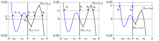
Figure 3. The graphs of $\sigma_{+}(k)$ (blue) and $\sigma_{-}(k)$ (black) when $\mu_{0}>1$ and $-\sigma_{c,1}<\sigma_{c,2}$. Left: When $0<\sigma<-\sigma_{c,1}$, $\sigma_{\pm}(k)=\sigma$ have six roots $k_{j}(\sigma)$, $j=1,2,\dots,6$. Middle: When $-\sigma_{c,1}<\sigma<\sigma_{c,2}$, $\sigma_{\pm}(k)=\sigma$ have four roots $k_{j}(\sigma)$, $j=2,4,5,6$. Right: When $\sigma>\sigma_{c,2}$, $\sigma_{\pm}(k)=\sigma$ have two roots $k_{j}(\sigma)$, $j=4,5$.

On the other hand, Figure 4 provides an example for the case $-\sigma_{c,1}>\sigma_{c,2}$. We do not include the discussion for the roots of $\sigma_{\pm}(k)=\sigma$. See Figure 6 to distinguish the region where $-\sigma_{c,1}>\sigma_{c,2}$ and the region where $-\sigma_{c,1}<\sigma_{c,2}$.

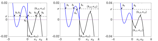
Figure 4. The graphs of $\sigma_{+}(k)$ (blue) and $\sigma_{-}(k)$ (black) when $\mu_{0}>1$ and $-\sigma_{c,1}>\sigma_{c,2}$. Left: When $0<\sigma<\sigma_{c,2}$, $\sigma_{\pm}(k)=\sigma$ have six roots $k_{j}(\sigma)$, $j=1,2,3,4,5,6$. Middle: When $\sigma_{c,2}<\sigma<-\sigma_{c,1}$, $\sigma_{\pm}(k)=\sigma$ have four roots $k_{j}(\sigma)$, $j=1,3,4,5$. Right: When $-\sigma_{c,1}<\sigma$, $\sigma_{\pm}(k)=\sigma$ have two roots $k_{j}(\sigma)$, $j=4,5$.

Lemma 3.5.

For $\mu_{0}\in(0,1)$, let $\kappa>0$ solve (2.5). Then, $\sigma_{-}(\kappa;\beta,\mu_{0})=0$. Moreover, there exists a critical point $k_{c}\in(0,\kappa)$ of $\sigma_{-}(\cdot;\beta,\mu_{0})$ on $(0,\infty)$ such that $\sigma_{-}(\cdot;\beta,\mu_{0})$ is strictly increasing on $(0,k_{c})$ and is strictly decreasing on $(k_{c},+\infty)$. If $\beta\in(0,\frac{1}{3})$, there exists an inflection point $k_{*}\in(0,k_{c})$ of $\sigma_{-}(\cdot;\beta,\mu_{0})$ on $(0,\infty)$ such that $\sigma_{-}(\cdot;\beta,\mu_{0})$ is convex on $(0,k_{*})$ and concave on $(k_{*},\infty)$. If $\beta\in[\frac{1}{3},+\infty)$, $\sigma_{-}(\cdot;\beta,\mu_{0})$ is concave on $(0,\infty)$.

Proof.

Again, the equation $\sigma_{-}(\kappa;\beta,\mu_{0})=0$ amounts to (2.5). The existence of critical points $k_{c}\in(0,\kappa)$ is guaranteed by Rolle’s Theorem. By the later proof of Lemma 3.4, $\frac{d\sigma_{-}}{dk}(k;\beta,\mu_{0})$ is positive on $(0,k_{c})$ and negative on $(k_{c},\infty)$ and the concavity of $\sigma_{-}(\cdot;\beta,\mu_{0})$ also follows easily. ∎

Under the consideration of Lemma 3.5, let $\sigma_{c}=\sigma_{-}(k_{c})$ be the unique critical value of $\sigma_{-}$. See Figure 5. We find that

• When $0\leqslant\sigma<\sigma_{c}$, $\sigma_{+}(k)=\sigma$ has two simple roots $k_{4}(\sigma)$ and $k_{5}(\sigma)$ satisfying $k_{5}(\sigma)\leqslant-\kappa<0\leqslant k_{4}(\sigma)$, and $\sigma_{-}(k)=\sigma$ has two simple roots $k_{2}(\sigma)$ and $k_{6}(\sigma)$ satisfying $0\leqslant k_{2}(\sigma)<k_{6}(\sigma)\leqslant\kappa$;

• When $\sigma=\sigma_{c}$, $\sigma_{-}(k)=\sigma_{c}$ has one double root at $k_{2}(\sigma_{c})=k_{6}(\sigma_{c})=k_{c}$, and $\sigma_{+}(k)=\sigma_{c}$ has two simple roots $k_{5}(\sigma_{c})<-\kappa<0<k_{4}(\sigma_{c})$;

• When $\sigma>\sigma_{c}$, $\sigma_{+}(k)=\sigma$ has two simple roots $k_{5}(\sigma)<-\kappa<0<k_{4}(\sigma)$, and $\sigma_{-}(k)=\sigma$ has no root.

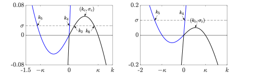
Figure 5. The graphs of $\sigma_{+}(k)$ (blue) and $\sigma_{-}(k)$ (black) when $\mu_{0}<1$. Left: When $0<\sigma<\sigma_{c}$, $\sigma_{\pm}(k)=\sigma$ have four roots $k_{j}(\sigma)$, $j=2,4,5,6$. Right: When $\sigma>\sigma_{c}$, $\sigma_{\pm}(k)=\sigma$ have two roots $k_{j}(\sigma)$, $j=4,5$.

Lemma 3.6 (Spectrum of $\mathbf{L}({i\sigma})$).

Let $(\beta,\kappa)$ be in the $S_{3}$ region of sub-critical waves. When $\sigma=0$, $ik_{j}(0)=(-1)^{j}i\kappa$, $j=5,6$, are simple eigenvalues of $\mathbf{L}(0):{\rm dom}(\mathbf{L})\subset Y\to Y$, and

$$\ker(\mathbf{L}(0)-ik_{j}(0)\mathbf{1}) =\ker((\mathbf{L}(0)-ik_{j}(0)\mathbf{1})^{2})={\rm span}\{\boldsymbol{\phi}_{j}(0)\},$$ (3.20)

$$\boldsymbol{\phi}_{j}(0) =\begin{pmatrix}\,{\rm ch}(k_{j}(0)y)\\ ik_{j}(0)\,{\rm ch}(k_{j}(0)y)\\ i\,{\rm sh}(k_{j}(0))\\ -\beta k_{j}(0)\,{\rm sh}(k_{j}(0))\end{pmatrix},$$

where $\mathbf{1}$ denotes the identity operator. Also, $ik_{j}(0)=0$, $j=2,4$, is an eigenvalue of $\mathbf{L}(0)$ with algebraic multiplicity $2$ and geometric multiplicity $1$, and

$$\ker(\mathbf{L}(0)^{2})=\ker(\mathbf{L}(0)^{3})={\rm span}\{\boldsymbol{\phi}_{2}(0),\boldsymbol{\phi}_{4}(0)\},$$

where

$$\boldsymbol{\phi}_{2}(0)=\begin{pmatrix}0\\ 1\\ \frac{1}{\mu_{0}}\\ 0\end{pmatrix}\quad\text{and}\quad\boldsymbol{\phi}_{4}(0)=\begin{pmatrix}1\\ 0\\ 0\\ 0\end{pmatrix}.$$ (3.21)

When $0<\sigma<\sigma_{c}$, $ik_{j}(\sigma)$, $j=2,4,5,6$, are simple eigenvalues of $\mathbf{L}(i\sigma)$, and

$$\ker(\mathbf{L}(i\sigma)-ik_{j}(\sigma)\mathbf{1})=\ker((\mathbf{L}(i\sigma)-ik_{j}(\sigma)\mathbf{1})^{2})={\rm span}\{\boldsymbol{\phi}_{j}(\sigma)\},$$

where

$$\boldsymbol{\phi}_{j}(\sigma)=\begin{pmatrix}\,{\rm ch}(k_{j}(\sigma)y)+\dfrac{k_{j}(\sigma)\sigma\,{\rm sh}(k_{j}(\sigma))y^{2}}{2(k_{j}(\sigma)-\sigma)}\\ ik_{j}(\sigma)\,{\rm ch}(k_{j}(\sigma)y)\\ \dfrac{ik_{j}(\sigma)\,{\rm sh}(k_{j}(\sigma))}{k_{j}(\sigma)-\sigma}\\ -\dfrac{\beta k_{j}(\sigma)^{2}\,{\rm sh}(k_{j}(\sigma))}{k_{j}(\sigma)-\sigma}\end{pmatrix}.$$ (3.22)

When $\sigma>\sigma_{c}$, $ik_{j}(\sigma)$, $j=4,5$, are simple eigenvalues of $\mathbf{L}(i\sigma)$, and (3.22) holds.

When $\sigma=\sigma_{c}$, $ik_{j}(\sigma_{c})$, $j=4,5$, are simple eigenvalues of $\mathbf{L}(i\sigma_{c})$, and (3.22) holds. Also, $ik_{c}$ is an eigenvalue with algebraic multiplicity $2$ and geometric multiplicity $1$, and

$$\ker((\mathbf{L}(i\sigma_{c})-ik_{c}\mathbf{1})^{2})=\ker((\mathbf{L}(i\sigma_{c})-ik_{c}\mathbf{1})^{3})={\rm span}\{\boldsymbol{\phi}_{2}(\sigma_{c}),\boldsymbol{\phi}_{6}(\sigma_{c})\}$$

and $(\mathbf{L}(i\sigma_{c})-ik_{c}\mathbf{1})\boldsymbol{\phi}_{6}(\sigma_{c})=\boldsymbol{\phi}_{2}(\sigma_{c})$, where $\boldsymbol{\phi}_{2}(\sigma_{c})$ is in (3.22) and

$$\boldsymbol{\phi}_{6}(\sigma_{c})$$ (3.23)

$$= \begin{pmatrix}-iy\,{\rm sh}(k_{c}y)+\dfrac{i\sigma_{c}(\sigma_{c}\,{\rm sh}(k_{c})-k_{c}^{2}\,{\rm ch}(k_{c})+k_{c}\sigma_{c}\,{\rm ch}(k_{c}))y^{2}}{2(k_{c}-\sigma_{c})^{2}}\\ \,{\rm ch}(k_{c}y)+k_{c}y\,{\rm sh}(k_{c}y)\\ -\dfrac{\sigma_{c}\,{\rm sh}(k_{c})-k_{c}^{2}\,{\rm ch}(k_{c})+k_{c}\sigma_{c}\,{\rm ch}(k_{c})}{(k_{c}-\sigma_{c})^{2}}\\ \dfrac{i\beta k_{c}(k_{c}\,{\rm sh}(k_{c})-2\sigma_{c}\,{\rm sh}(k_{c})+k_{c}^{2}\,{\rm ch}(k_{c})-k_{c}\sigma_{c}\,{\rm ch}(k_{c}))}{(k_{c}-\sigma_{c})^{2}}\end{pmatrix}.$$

Let $(\beta,\kappa)$ be in the super-critical region with $-\sigma_{c,1}<\sigma_{c,2}$, when $\sigma=0$ $ik_{j}(0)=(-1)^{j}i\kappa$, $j=1,2,5,6$, are simple eigenvalues of $\mathbf{L}(0):{\rm dom}(\mathbf{L})\subset Y\to Y$, and (3.20) holds. Also, $ik_{j}(0)=0$, $j=3,4$, is an eigenvalue of $\mathbf{L}(0)$ with algebraic multiplicity $2$ and geometric multiplicity $1$, and

$$\ker(\mathbf{L}(0)^{2})=\ker(\mathbf{L}(0)^{3})={\rm span}\{\boldsymbol{\phi}_{3}(0),\boldsymbol{\phi}_{4}(0)\},$$

where

$$\boldsymbol{\phi}_{3}(0)=\begin{pmatrix}0\\ 1\\ 1/\mu_{0}\\ 0\end{pmatrix}\quad\text{and}\quad\boldsymbol{\phi}_{4}(0)=\begin{pmatrix}1\\ 0\\ 0\\ 0\end{pmatrix}.$$ (3.24)

When $0<\sigma<-\sigma_{c,1}$, $ik_{j}(\sigma)$, $j=1,2,3,4,5,6$, are simple eigenvalues of $\mathbf{L}(i\sigma)$, and (3.22) holds.

When $\sigma=-\sigma_{c,1}$, $ik_{j}(\sigma)$, $j=2,4,5,6$, are simple eigenvalues of $\mathbf{L}(i\sigma)$, and (3.22) holds. $-ik_{c,1}$ is a double eigenvalue of $\mathbf{L}(i\sigma)$, and (LABEL:generalized_eigenvector) holds with $k_{c}$ and $\sigma_{c}$ replaced by $-k_{1,c}$ and $-\sigma_{c,1}$, respectively.

When $-\sigma_{c,1}<\sigma<\sigma_{c,2}$, $ik_{j}(\sigma)$, $j=2,4,5,6$, are simple eigenvalues of $\mathbf{L}(i\sigma)$, and (3.22) holds.

When $\sigma=\sigma_{c,2}$, $ik_{j}(\sigma)$, $j=4,5$, are simple eigenvalues of $\mathbf{L}(i\sigma)$, and (3.22) holds. $ik_{c,2}$ is a double eigenvalue of $\mathbf{L}(i\sigma)$, and (LABEL:generalized_eigenvector) holds with $k_{c}$ and $\sigma_{c}$ replaced by $k_{2,c}$ and $\sigma_{c,2}$, respectively.

When $\sigma_{c,2}<\sigma$, $ik_{j}(\sigma_{c})$, $j=4,5$, are simple eigenvalues of $\mathbf{L}(i\sigma)$, and (3.22) holds.

We omit the discussion for $(\beta,\kappa)$ in the super-critical region with $-\sigma_{c,1}>\sigma_{c,2}$.

The proof of Lemma 3.6 follows from a straightforward calculation and we do not include the details here. See [17, Appendix C] for gravity waves.

Definition 3.7 (Eigenspace and projection).

Let $\sigma\geqslant 0$, and $Y(\sigma)$ denote the eigenspace of $\mathbf{L}(i\sigma):{\rm dom}(\mathbf{L})\subset Y\to Y$ associated with its finitely many and purely imaginary eigenvalues. Let

$$\boldsymbol{\Pi}(\sigma):{\rm dom}(\mathbf{L})\subset Y\to Y(\sigma)$$

be the projection of ${\rm dom}(\mathbf{L})$ onto $Y(\sigma)$, which commutes with $\mathbf{L}(i\sigma)$. Based on Lemma 3.6, we choose an ordered basis $\mathcal{B}(\sigma)$ of $Y(\sigma)$ as follow:
In the sub-critical region,

• when $\sigma=0$, $\mathcal{B}(0):=\{\boldsymbol{\phi}_{j}(0):j=5,6,2,4\}$, where $\boldsymbol{\phi}_{j}(0)$ is in (3.20) and (3.21);

• when $0<\sigma<\sigma_{c}$, $\mathcal{B}(\sigma):=\{\boldsymbol{\phi}_{j}(\sigma):j=2,4,5,6\}$, where $\boldsymbol{\phi}_{j}(\sigma)$ is in (3.22);

• when $\sigma=\sigma_{c}$, $\mathcal{B}(\sigma):=\{\boldsymbol{\phi}_{j}(\sigma):j=2,4,5,6\}$, where, for $j=2,4,5$, $\boldsymbol{\phi}_{j}(\sigma)$ is in (3.22) and $\boldsymbol{\phi}_{6}(\sigma)$ is in (LABEL:generalized_eigenvector);

• when $\sigma>\sigma_{c}$, $\mathcal{B}(\sigma):=\{\boldsymbol{\phi}_{j}(\sigma):j=4,5\}$, where $\boldsymbol{\phi}_{j}(\sigma)$ is in (3.22).

In the super-critical region with $-\sigma_{c,1}<\sigma_{c,2}$,

• when $\sigma=0$, $\mathcal{B}(0):=\{\boldsymbol{\phi}_{j}(0):j=1,2,3,4,5,6\}$, where $\boldsymbol{\phi}_{j}(0)$ is in (3.20) and (3.24);

• when $0<\sigma<-\sigma_{c,1}$, $\mathcal{B}(\sigma):=\{\boldsymbol{\phi}_{j}(\sigma):j=1,2,3,4,5,6\}$, where $\boldsymbol{\phi}_{j}(\sigma)$ is in (3.22);

• when $-\sigma_{c,1}<\sigma<\sigma_{c,2}$, $\mathcal{B}(\sigma):=\{\boldsymbol{\phi}_{j}(\sigma_{c}):j=2,4,5,6\}$, where $\boldsymbol{\phi}_{j}(\sigma)$ is in (3.22);

• when $\sigma>\sigma_{c,2}$, $\mathcal{B}(\sigma):=\{\boldsymbol{\phi}_{j}(\sigma):j=4,5\}$, where $\boldsymbol{\phi}_{j}(\sigma)$ is in (3.22).

We omit the discussion for $\sigma=-\sigma_{c,1}$ and $\sigma=\sigma_{c,2}$ and the discussion for super-critical region with $-\sigma_{c,1}\geqslant\sigma_{c,2}$. The formulas of $\boldsymbol{\Pi}(\sigma)$ are in Section 3.5.

By symmetry, $ik_{j}(\sigma)=-ik_{j}(-\sigma)$, whereby Lemma 3.6 and Definition 3.7 extend to $\sigma<0$.

3.4. Reduction of the spectral problem. The periodic Evans function

We turn the attention to $|\varepsilon|\neq 0,\ll 1$. Let

$$\lambda=i\sigma+\delta,\quad\text{where}\quad\sigma\in\mathbb{R},\quad\delta\in\mathbb{C}\quad\text{and}\quad|\delta|\ll 1,$$

and we rewrite (3.10) as

$$\mathbf{u}_{x} =\mathbf{L}(i\sigma)\mathbf{u}+(\mathbf{L}(i\sigma+\delta)-\mathbf{L}(i\sigma))\mathbf{u}+\mathbf{B}(x;i\sigma+\delta,\varepsilon)\mathbf{u}(x)$$ (3.25)

$$=:\mathbf{L}(i\sigma)\mathbf{u}+\mathbf{B}(x;\sigma,\delta,\varepsilon)\mathbf{u}(x),$$

where $\mathbf{L}(i\sigma):{\rm dom}(\mathbf{L})\subset Y\to Y$ is in (3.11), (3.12), (3.13), and

$$\mathbf{B}(x;\sigma,\delta,\varepsilon):\mathbb{R}\times{\rm dom}(\mathbf{L})\subset\mathbb{R}\times Y\to Y.$$

Notice that $\mathbf{B}(x;\sigma,\delta,\varepsilon)$ is smooth and $T(=2\pi/\kappa)$ periodic in $x$, and it depends analytically on $\sigma$, $\delta$ and $\varepsilon$. Also, $\mathbf{B}(x;\sigma,0,0)=\mathbf{0}$. Our proofs do not involve all the details of $\mathbf{B}(x;\sigma,\delta,\varepsilon)$, and rather its leading order terms as $\delta,\varepsilon\to 0$, whence we do not include the formulas here. But see, for instance, (3.54) and Appendix C (C.1)- (LABEL:eqn:B02).

For $\mathbf{u}(x)\in{\rm dom}(\mathbf{L})$, $x\in\mathbb{R}$, let

$$\mathbf{v}(x)=\boldsymbol{\Pi}(\sigma)\mathbf{u}(x)\quad\text{and}\quad\mathbf{w}(x)=(\mathbf{1}-\boldsymbol{\Pi}(\sigma))\mathbf{u}(x),$$

where $\mathbf{1}$ denotes the identity operator, and (3.25) becomes

$${\mathbf{v}}_{x}= \mathbf{L}(i\sigma)\mathbf{v}+\boldsymbol{\Pi}(\sigma)\mathbf{B}(x;\sigma,\delta,\varepsilon)(\mathbf{v}(x)+\mathbf{w}(x)),$$ (3.26)

$${\mathbf{w}}_{x}= \mathbf{L}(i\sigma)\mathbf{w}+(\mathbf{1}-\boldsymbol{\Pi}(\sigma))\mathbf{B}(x;\sigma,\delta,\varepsilon)(\mathbf{v}(x)+\mathbf{w}(x)).$$

Recall from discussion above that $Y(\sigma)$ is finite dimensional. Our setup (3.25), or equivalently (3.26), satisfies hypotheses (A1) and (A2) of Mielke’s reduction theorem [26, Theorem 1]. To verify the last critical hypothesis (A3) for resolvent estimates, we refer to, for instance, [18, Lemma 2.1], [7, Prop. 3.2], [6, Prop. 2], and [15, Lemma 3.4] , to learn that the task is accomplished by the following lemma.

Lemma 3.8.

For a fixed $\sigma\in\mathbb{R}$, a complex number $ik$ is an eigenvalue of $\mathbf{L}(i\sigma)$ if and only if $k$ solves the latter equation of (3.18). There exist $k_{0}(\sigma)>0$ and $C(\sigma)>0$ both sufficiently large such that, for all $k>k_{0}(\sigma)$, $ik$ lies in the resolvent set of $\mathbf{L}(i\sigma)$ and

$$||(ik{\rm Id}-\mathbf{L}(i\sigma))^{-1}||_{Y\rightarrow Y}\leqslant\frac{C(\sigma)}{k}.$$ (3.27)

Proof.

Our computations in former sections have shown the foregoing claim. Recall $\mathbf{L}(i\sigma)$ has compact resolvent, so that the spectrum consists (entirely) of discrete eigenvalues with finite multiplicities, which are shown to be bounded on the imaginary axis. For all sufficiently large $k\in\mathbb{R}$, the pure imaginary number $ik$ thus belongs to the resolvent set. To obtain the bound (3.27) for the inverse operator, consider the resolvent equations

$$(ik{\rm Id}-\mathbf{L}(i\sigma))\mathbf{u}=\mathbf{f}_{*}=\begin{pmatrix}\phi_{*}\\ u_{*}\\ \eta_{*}\\ z_{*}\end{pmatrix}.$$

The first equation reads

$$-u+ik\phi=\phi_{*}-\frac{i\sigma z}{2\beta}y^{2}.$$

Taking square of $||\cdot||_{H^{1}}$ norm on both hand sides and using

$$|a+ikb|^{2}=|a|^{2}+k^{2}|b|^{2}+2k\Im(a\bar{b}),\quad\text{for $a,b\in\mathbb{C},k\in\mathbb{R}$,}$$

yields

$$||u||_{H^{1}}^{2}+k^{2}||\phi||_{H^{1}}^{2}-2k\Im\langle u,\phi\rangle-2k\Im\langle u_{y},\phi_{y}\rangle$$

$$= ||-u+ik\phi||_{H^{1}}^{2}=||\phi_{*}-\frac{i\sigma z}{2\beta}y^{2}||_{H^{1}}^{2}$$

$$\leqslant 2||\phi_{*}||_{H^{1}}^{2}+2||\frac{i\sigma z}{2\beta}y^{2}||_{H^{1}}^{2}=2||\phi_{*}||_{H^{1}}^{2}+\frac{23\sigma^{2}}{15\beta^{2}}|z|^{2},$$

whence

$$||u||_{H^{1}}^{2}+k^{2}||\phi||_{H^{1}}^{2}\leqslant 2||\phi_{*}||_{H^{1}}^{2}+\frac{23\sigma^{2}}{15\beta^{2}}|z|^{2}+2k\Im\langle u,\phi\rangle+2k\Im\langle u_{y},\phi_{y}\rangle.$$ (3.28)

By Young’s inequality, there holds

$$2k\Im\langle u,\phi\rangle\leqslant\frac{1}{\varepsilon_{1}}||\phi||_{L^{2}}^{2}+\varepsilon_{1}k^{2}||u||_{L^{2}}^{2}.$$ (3.29)

To bound $2k\Im\langle u_{y},\phi_{y}\rangle$, integration by part, we find

$$2k\Im\langle u_{y},\phi_{y}\rangle=2k\Im\left(u(1)\overline{\Phi_{y}(1)}-\langle u,\phi_{yy}\rangle\right)$$ (3.30)

$$= -2k\Im\left(\mu_{0}z_{*}+\mu_{0}\eta+i\sigma\phi(1)-\tfrac{1}{2}\sigma^{2}\eta-ik\mu_{0}z\right)\frac{\bar{z}}{\beta}$$

$$-2k\Im\langle u,u_{*}-iku-i\sigma\eta\rangle$$

$$= -2k\Im\left(\mu_{0}z_{*}+\mu_{0}\eta+i\sigma\phi(1)-\tfrac{1}{2}\sigma^{2}\eta\right)\frac{\bar{z}}{\beta}$$

$$-2k\Im\langle u,u_{*}-i\sigma\eta\rangle-\frac{2\mu_{0}k^{2}}{\beta}|z|^{2}-2k^{2}||u||_{L^{2}}^{2}$$

where we have made substitutions by (i) the fourth equation of the resolvent equations $u(1)=\mu_{0}z_{*}+\mu_{0}\eta+i\sigma\phi(1)-\tfrac{1}{2}\sigma^{2}\eta-ik\mu_{0}z$, (ii) the second equation of the resolvent equations $\phi_{yy}=u_{*}-iku-i\sigma\eta$, and the boundary condition $\phi_{y}(1)=-\frac{z}{\beta}$. Applying Young’s inequality to the right hand side of (LABEL:estimate3) yields

$$2k\Im\langle u_{y},\phi_{y}\rangle\leqslant \frac{\mu_{0}^{2}}{\beta^{2}\varepsilon_{2}}|z_{*}|^{2}+\varepsilon_{2}k^{2}|z|^{2}+\frac{(\mu_{0}-\tfrac{1}{2}\sigma^{2})^{2}}{\beta^{2}\varepsilon_{3}}|\eta|^{2}$$ (3.31)

$$+\varepsilon_{3}k^{2}|z|^{2}+\frac{\sigma^{2}}{\beta^{2}\varepsilon_{4}}|\phi(1)|^{2}+\varepsilon_{4}k^{2}|z|^{2}$$

$$+\frac{1}{\varepsilon_{5}}||u_{*}||_{L^{2}}^{2}+\varepsilon_{5}k^{2}||u||_{L^{2}}^{2}+\frac{\sigma^{2}}{\varepsilon_{6}}|\eta|^{2}$$

$$+\varepsilon_{6}k^{2}||u||_{L^{2}}^{2}-\frac{2\mu_{0}k^{2}}{\beta}|z|^{2}-2k^{2}||u||_{L^{2}}^{2}$$

$$\leqslant \frac{1}{\varepsilon_{5}}||u_{*}||_{L^{2}}^{2}+\frac{\mu_{0}^{2}}{\beta^{2}\varepsilon_{2}}|z_{*}|^{2}+\frac{\sigma^{2}c}{\beta^{2}\varepsilon_{4}}||\phi||_{H^{1}}^{2}$$

$$+(-2+\varepsilon_{5}+\varepsilon_{6})k^{2}||u||_{L^{2}}^{2}$$

$$+\left(\frac{(\mu_{0}-\tfrac{1}{2}\sigma^{2})^{2}}{\beta^{2}\varepsilon_{3}}+\frac{\sigma^{2}}{\varepsilon_{6}}\right)|\eta|^{2}$$

$$+(-\frac{2\mu_{0}}{\beta}+\varepsilon_{2}+\varepsilon_{3}+\varepsilon_{4})k^{2}|z|^{2},$$

where, in the last inequality, we have used Morrey’s inequality $|\phi(1)|\leqslant|\phi|_{C([0,1])}\leqslant c||\phi||_{H^{1}}$. Here $c$ is a constant. Using (3.29) and (3.31) in (3.28), we obtain

$$\left(k^{2}-\frac{1}{\varepsilon_{1}}-\frac{\sigma^{2}c}{\beta^{2}\varepsilon_{4}}\right)||\phi||_{H^{1}}^{2}+(2-\varepsilon_{1}-\varepsilon_{5}-\varepsilon_{6})k^{2}||u||_{L^{2}}^{2}+||u||_{H^{1}}^{2}$$ (3.32)

$$+\left((\frac{2\mu_{0}}{\beta}-\varepsilon_{2}-\varepsilon_{3}-\varepsilon_{4})k^{2}-\frac{23\sigma^{2}}{15\beta^{2}}\right)|z|^{2}$$

$$\leqslant 2||\phi_{*}||_{H^{1}}^{2}+\frac{1}{\varepsilon_{5}}||u_{*}||_{L^{2}}^{2}+\frac{\mu_{0}^{2}}{\beta^{2}\varepsilon_{2}}|z_{*}|^{2}+\left(\frac{(\mu_{0}-\tfrac{1}{2}\sigma^{2})^{2}}{\beta^{2}\varepsilon_{3}}+\frac{\sigma^{2}}{\varepsilon_{6}}\right)|\eta|^{2}.$$

By the third equation $-\frac{z}{\beta}+ik\eta=\eta_{*}$, we find $\frac{1}{\beta^{2}}|z|^{2}+k^{2}|\eta|^{2}-2k\Im(\frac{z}{\beta}\bar{\eta})=|\eta_{*}|^{2}$, whence

$$\frac{1}{\beta^{2}}|z|^{2}+k^{2}|\eta|^{2}\leqslant|\eta_{*}|^{2}+\frac{1}{\beta^{2}\varepsilon_{7}}|z|^{2}+\varepsilon_{7}k^{2}|\eta|^{2}.$$ (3.33)

Taking the sum of (LABEL:estimate5) and (3.33) yields

$$\left(k^{2}-\frac{1}{\varepsilon_{1}}-\frac{\sigma^{2}c}{\beta^{2}\varepsilon_{4}}\right)||\phi||_{H^{1}}^{2}+(2-\varepsilon_{1}-\varepsilon_{5}-\varepsilon_{6})k^{2}||u||_{L^{2}}^{2}$$ (3.34)

$$+\left((1-\varepsilon_{7})k^{2}-\frac{(\mu_{0}-\tfrac{1}{2}\sigma^{2})^{2}}{\beta^{2}\varepsilon_{3}}-\frac{\sigma^{2}}{\varepsilon_{6}}\right)|\eta|^{2}$$

$$+\left((\frac{2\mu_{0}}{\beta}-\varepsilon_{2}-\varepsilon_{3}-\varepsilon_{4})k^{2}-\frac{23\sigma^{2}}{15\beta^{2}}+\frac{1}{\beta^{2}}-\frac{1}{\beta^{2}\varepsilon_{7}}\right)|z|^{2}$$

$$\leqslant 2||\phi_{*}||_{H^{1}}^{2}+\frac{1}{\varepsilon_{5}}||u_{*}||_{L^{2}}^{2}+|\eta_{*}|^{2}+\frac{\mu_{0}^{2}}{\beta^{2}\varepsilon_{2}}|z_{*}|^{2}.$$

Choosing $\varepsilon_{1},\varepsilon_{5},\varepsilon_{6}=\frac{1}{3}$, $\varepsilon_{2},\varepsilon_{3},\varepsilon_{4}=\frac{\mu_{0}}{3\beta}$, and $\varepsilon_{7}=\frac{1}{2}$, there exist $k_{0}(\sigma,\beta,\mu_{0},c)$ and $C(\sigma,\beta,\mu_{0},c)$ such that for $k>k_{0}(\sigma,\beta,\mu_{0},c)$

$$k^{2}\left(||\phi||_{H^{1}}^{2}+||u||_{L^{2}}^{2}+|\eta|^{2}+|z|^{2}\right)$$ (3.35)

$$\leqslant C(\sigma,\beta,\mu_{0},c)\left(||\phi_{*}||_{H^{1}}^{2}+||u_{*}||_{L^{2}}^{2}+|\eta_{*}|^{2}+|z_{*}|^{2}\right),$$

yielding (3.27). ∎

The reduction theorem of Mielke’s [26, Theorem 1] asserts, for $\sigma\in\mathbb{R}$, $\delta\in\mathbb{C}$ and $|\delta|\ll 1$, for $\varepsilon\in\mathbb{R}$ and $|\varepsilon|\ll 1$, there exists

$$\mathbf{w}(x,\mathbf{v}(x);\sigma,\delta,\varepsilon):\mathbb{R}\times Y(\sigma)\to{\rm dom}(\mathbf{L})$$ (3.36)

such that $\mathbf{v}+\mathbf{w}$ makes a bounded solution of (3.25), hence (3.10), if and only if $\mathbf{v}$ makes a bounded solution of the reduced system

$${\mathbf{v}}_{x}=\mathbf{L}(i\sigma)\mathbf{v}+\boldsymbol{\Pi}(\sigma)\mathbf{B}(x;\sigma,\delta,\varepsilon)(\mathbf{v}(x)+\mathbf{w}(x,\mathbf{v}(x);\sigma,\delta,\varepsilon)).$$ (3.37)

Therefore, we turn (3.25), for which $\mathbf{u}(x)\in{\rm dom}(\mathbf{L})$, $x\in\mathbb{R}$, and $\dim({\rm dom}(\mathbf{L}))=\infty$, into (3.37), for which $\mathbf{v}(x)\in Y(\sigma)$ and $\dim(Y(\sigma))<\infty$.

For $\mathbf{v}(x)\in Y(\sigma)$, $x\in\mathbb{R}$, let $\mathbf{a}(x)$ be the coordinate of $\mathbf{v}(x)$ with respect to the ordered basis $\mathcal{B}(\sigma)$ of $Y(\sigma)$, i.e.,

$$\mathbf{v}(x)=\mathcal{B}(\sigma)\mathbf{a}(x),$$

and we may further rewrite (3.37) as

$$\mathbf{a}_{x}=\mathbf{A}(x;\sigma,\delta,\varepsilon)\mathbf{a},$$ (3.38)

where $\mathbf{A}(x;\sigma,\delta,\varepsilon)$ is a square matrix of order $2$ or $4$ or $6$ depending on $\sigma$ and $\mu_{0}$. Notice that $\mathbf{A}(x;\sigma,\delta,\varepsilon)$ is smooth and $T(=2\pi/k)$ periodic in $x$, and it depends analytically on $\delta$ and $\varepsilon$. Our proofs do not involve all the details of $\mathbf{A}(x;\sigma,\delta,\varepsilon)$, and rather its leading order terms as $\delta,\varepsilon\to 0$, whence we do not include the formula here. But see, for instance, (LABEL:eqn:a), (3.57) and (3.59), (3.60). By Floquet theory, if $\mathbf{a}$ is a bounded solution of (3.38) then, necessarily,

$$\mathbf{a}(x+T)=e^{ikT}\mathbf{a}(x)\quad\text{for some $k\in\mathbb{R}$},\quad\text{where $T=2\pi/\kappa$}$$

is the period of the underlying wave.

Following [13, 14] and others, we take a periodic Evans function approach.

Definition 3.9 (The periodic Evans function).

For $\lambda=i\sigma+\delta$, $\sigma\in\mathbb{R}$, $\delta\in\mathbb{C}$ and $|\delta|\ll 1$, for $\varepsilon\in\mathbb{R}$ and $|\varepsilon|\ll 1$, let $\mathbf{X}(x;\sigma,\delta,\varepsilon)$ denote the fundamental solution of (3.38) such that $\mathbf{X}(0;\sigma,\delta,\varepsilon)=\mathbf{I}$, where $\mathbf{I}$ is the identity matrix. Let $\mathbf{X}(T;\sigma,\delta,\varepsilon)$ be the monodromy matrix for (3.38), and for $k\in\mathbb{R}$,

$$\Delta(\lambda,k;\varepsilon)=\det(e^{ikT}\mathbf{I}-\mathbf{X}(T;\sigma,\delta,\varepsilon))$$ (3.39)

the periodic Evans function, where $T=2\pi/\kappa$ is the period of the wave.

Since $\mathbf{A}(x;\sigma,\delta,\varepsilon)$ depends analytically on $\sigma$, $\delta$ and $\epsilon$ for any $x\in\mathbb{R}$, so do $\mathbf{X}(T;\sigma,\delta,\varepsilon)$ and, hence, $\Delta(\lambda,k;\varepsilon)$ depends analytically on $\lambda$, $k$ and $\varepsilon$, where $\lambda=i\sigma+\delta$ and $k\in\mathbb{R}$. By Floquet theory and [26, Theorem 1], for instance, for $\varepsilon\in\mathbb{R}$ and $|\varepsilon|\ll 1$, $\lambda\in{\rm spec}(\mathcal{L}(\varepsilon))$ if and only if

$$\Delta(\lambda,k;\varepsilon)=0\quad\text{for some $k\in\mathbb{R}$}.$$

See [13], for instance, for more details.

Remark.

A $(\beta,\kappa)$-wave of sufficiently small amplitude is spectrally stable if and only if

$${\rm spec}(\mathcal{L}(\varepsilon))=\{\lambda\in\mathbb{C}:\Delta(\lambda,k;\varepsilon)=0\quad\text{for some $k\in\mathbb{R}$}\}\subset i\mathbb{R}$$

for $\varepsilon\in\mathbb{R}$ and $|\varepsilon|\ll 1$.

In what follows, we identify ${\rm spec}(\mathcal{L}(\varepsilon))$ with the roots of the periodic Evans function.

One should not expect to be able to evaluate the periodic Evans function except for few cases, for instance, completely integrable PDEs. When $\varepsilon\in\mathbb{R}$ and $|\varepsilon|\ll 1$, on the other hand, we shall use the result of Section 2 and determine (3.39) for $|\varepsilon|\ll 1$.

Corollary 3.10 (spectrum of $\mathcal{L}(0)$, dispersion relation).

For constant wave $\varepsilon=0$, the periodic Evans function (3.39) satisfies

$$\Delta(i\sigma,k_{j}(\sigma);0)=0,\quad\text{for index $j$ satisfying $\boldsymbol{\phi}_{j}(\sigma)\in\mathcal{B}(\sigma)$.}$$ (3.40)

Proof.

When setting $\delta=\varepsilon=0$, because $\mathbf{B}(x;\sigma,0,0)=0$, (3.37) reduces to ${\mathbf{v}}_{x}=\mathbf{L}(i\sigma)\mathbf{v}$ whose solutions are discussed in Section 3.3. ∎

We thereby study the nearby root $(i\sigma+\delta,k_{j}(\sigma)+\gamma,\varepsilon)$ of the periodic Evans function $\Delta$ (3.39) for $\delta\in\mathbb{C}$, $\gamma,\varepsilon\in\mathbb{R}$ and $|\delta|,|\gamma|,|\varepsilon|\ll 1$. To prepare for the expansion of the periodic Evans function $\Delta(i\sigma+\delta,k_{j}(\sigma)+\gamma,\varepsilon)$ as series of $\delta$, $\gamma$, $\varepsilon$, we first make some necessary computations below.

3.5. Computation of $\boldsymbol{\Pi}(\sigma)$

For $\mathbf{u}_{1}:=\begin{pmatrix}\phi_{1}\\ u_{1}\\ \eta_{1}\\ z_{1}\end{pmatrix},\mathbf{u}_{2}:=\begin{pmatrix}\phi_{2}\\ u_{2}\\ \eta_{2}\\ z_{2}\end{pmatrix}\in Y$, we take the standard inner product on $Y$:

$$\langle\mathbf{u}_{1},\mathbf{u}_{2}\rangle=\int^{1}_{0}(\phi_{1}\phi_{2}^{*}+{\phi_{1}}_{y}{\phi_{2}}_{y}^{*})~{}dy+\int^{1}_{0}u_{1}u_{2}^{*}~{}dy+\eta_{1}\eta_{2}^{*}+z_{1}z_{2}^{*},$$ (3.41)

where the asterisk means complex conjugation. We then make a straightforward calculation and obtain, for $\mathbf{u}:=\begin{pmatrix}\phi\\ u\\ \eta\\ z\end{pmatrix},$

$$\mathbf{L}(\lambda)^{\dagger}:{\rm dom}(\mathbf{L}^{\dagger})\subset Y\to Y,$$

where

$$L(\lambda)^{\dagger}\mathbf{u}=\begin{pmatrix}u+\phi_{p}\\ -\phi_{yy}+\phi\\ \left(1+\frac{{\lambda^{*}}^{2}}{2\mu_{0}}\right)z-\lambda^{*}\int_{0}^{1}u\\ \frac{u(1)+\eta}{\beta}-\frac{\lambda^{*}}{2\beta}\int_{0}^{1}\left(y^{2}\phi+2y{\phi_{2}}_{y}\right)\end{pmatrix},$$

$$\phi_{p}(y)= \left(\lambda^{*}z/\mu_{0}-\int_{0}^{1}\,{\rm ch}(1-y)u(y)~{}dy\right)\frac{\,{\rm ch}(y)}{\,{\rm sh}(1)}$$ (3.42)

$$+\int_{0}^{y}\,{\rm sh}(y-y^{\prime})u(y^{\prime})~{}dy^{\prime},$$

and

$${\rm dom}(\mathbf{L}^{\dagger})=\{\mathbf{u}\in H^{2}(0,1)\times H^{1}(0,1)\times\mathbb{C}\times\mathbb{C}:\phi_{y}(1)-z/\mu_{0}=0,\phi_{y}(0)=0\},$$

which is dense in $Y$. We proceed to compute the projection $\boldsymbol{\Pi}(\sigma)$ in the sub-critical region.

When $\sigma=0$,

$$\boldsymbol{\Pi}(0)\mathbf{u}= \langle\mathbf{u},\boldsymbol{\psi}_{2}(0)\rangle\boldsymbol{\phi}_{2}(0)+\langle\mathbf{u},\boldsymbol{\psi}_{4}(0)\rangle\boldsymbol{\phi}_{4}(0)$$ (3.43)

$$+\langle\mathbf{u},\boldsymbol{\psi}_{5}(0)\rangle\boldsymbol{\phi}_{5}(0)+\langle\mathbf{u},\boldsymbol{\psi}_{6}(0)\rangle\boldsymbol{\phi}_{6}(0),$$

where, for $j=5,6$,

$$\boldsymbol{\psi}_{j}(0)=\begin{pmatrix}\frac{k_{j}\,{\rm sh}(k_{j})\,{\rm ch}(y)-k_{j}^{2}\,{\rm sh}(1)\,{\rm ch}(k_{j}y)}{\,{\rm sh}(1)(k_{j}^{2}-1)(k_{j}^{2}-\mu_{0}\,{\rm sh}(k_{j})^{2}+\beta k_{j}^{2}\mu_{0}\,{\rm sh}(k_{j})^{2})}\\ \frac{ik_{j}\,{\rm ch}(k_{j}y)}{k_{j}^{2}-\mu_{0}\,{\rm sh}(k_{j})^{2}+\beta k_{j}^{2}\mu_{0}\,{\rm sh}(k_{j})^{2}}\\ -\frac{i\mu_{0}\,{\rm sh}(k_{j})}{k_{j}^{2}-\mu_{0}\,{\rm sh}(k_{j})^{2}+\beta k_{j}^{2}\mu_{0}\,{\rm sh}(k_{j})^{2}}\\ -\frac{k_{j}\mu_{0}\,{\rm sh}(k_{j})}{k_{j}^{2}-\mu_{0}\,{\rm sh}(k_{j})^{2}+\beta k_{j}^{2}\mu_{0}\,{\rm sh}(k_{j})^{2}}\end{pmatrix},$$ (3.44)

and

$$\boldsymbol{\psi}_{2}=\begin{pmatrix}0\\ \mu_{0}/(\mu_{0}-1)\\ -\mu_{0}/(\mu_{0}-1)\\ 0\end{pmatrix},\quad\boldsymbol{\psi}_{4}=\begin{pmatrix}\frac{\mu_{0}}{\mu_{0}-1}-\frac{\,{\rm ch}(y)}{\,{\rm sh}(1)(\mu_{0}-1)}\\ 0\\ 0\\ -\frac{\mu_{0}}{\mu_{0}-1}\end{pmatrix}.$$ (3.45)

Remark.

The first entry of (3.44) appears to be not defined when $\kappa=1$. However, a straightforward calculation leads to that

$$\lim_{\kappa\to 1} \frac{\displaystyle\,{\rm sh}(\kappa)\,{\rm ch}(y)-\kappa\,{\rm sh}(1)\,{\rm ch}(\kappa y)}{1-\kappa}=y\,{\rm sh}(1)\,{\rm sh}(y)+\,{\rm sh}(1)\,{\rm ch}(y)-\,{\rm ch}(1)\,{\rm ch}(y)$$

is well defined. Thus we may define $\boldsymbol{\psi}_{j}(0)={\displaystyle\lim_{\kappa\to 1}\boldsymbol{\psi}_{j}(0)}$, $j=5,6$, when $\kappa=1$, and verify that $\langle\boldsymbol{\phi}_{j}(0),\boldsymbol{\psi}_{j^{\prime}}(0)\rangle=\delta_{jj^{\prime}}$, $j,j^{\prime}=2,4,5,6$.

When $0<\sigma\neq\sigma_{c}$, we infer from Lemma 3.6 that $-ik_{j}(\sigma)$, for indexes $j$ satisfying $\boldsymbol{\phi}_{j}(\sigma)\in\mathcal{B}(\sigma)$, are simple eigenvalues of $\mathbf{L}(i\sigma)^{\dagger}$, and a straightforward calculation reveals that the corresponding eigenfunctions are

$$\boldsymbol{\psi}_{j}(\sigma)=\begin{pmatrix}p_{1,j}\,{\rm ch}(k_{j}y)+p_{2,j}\,{\rm ch}(y)\\ i(1-k_{j}^{2})p_{1,j}\,{\rm ch}(k_{j}y)/k_{j}\\ p_{3,j}\\ \mu_{0}(k_{j}p_{1,j}\,{\rm sh}(k_{j})+p_{2,j}\,{\rm sh}(1))\end{pmatrix},$$ (3.46)

where

$$p_{1,j}= k_{j}\,{\rm sh}(k_{j})(k_{j}-\sigma)(\beta k_{j}^{2}+1)\cdot\big{(}(k_{j}^{2}-1)(\sigma\,{\rm ch}(k_{j})^{3}$$ (3.47)

$$-k_{j}^{2}\,{\rm sh}(k_{j})-k_{j}\,{\rm ch}(k_{j})-\sigma\,{\rm ch}(k_{j})+k_{j}\,{\rm ch}(k_{j})^{3}$$

$$+k_{j}\sigma\,{\rm sh}(k_{j})+\beta k_{j}^{3}\,{\rm ch}(k_{j})-\beta k_{j}^{4}\,{\rm sh}(k_{j})-\beta k_{j}^{3}\,{\rm ch}(k_{j})^{3}$$

$$+3\beta k_{j}^{2}\sigma\,{\rm ch}(k_{j})^{3}-3\beta k_{j}^{2}\sigma\,{\rm ch}(k_{j})+\beta k_{j}^{3}\sigma\,{\rm sh}(k_{j}))\big{)}^{-1},$$

$$p_{2,j}= k_{j}\,{\rm sh}(k_{j})^{2}(k_{j}\sigma-1)(\beta k_{j}^{2}+1)\cdot\big{(}\,{\rm sh}(1)(k_{j}^{2}-1)(\sigma\,{\rm ch}(k_{j})^{3}$$

$$-k_{j}^{2}\,{\rm sh}(k_{j})-k_{j}\,{\rm ch}(k_{j})-\sigma\,{\rm ch}(k_{j})+k_{j}\,{\rm ch}(k_{j})^{3}$$

$$+k_{j}\sigma\,{\rm sh}(k_{j})+\beta k_{j}^{3}\,{\rm ch}(k_{j})-\beta k_{j}^{4}\,{\rm sh}(k_{j})-\beta k_{j}^{3}\,{\rm ch}(k_{j})^{3}$$

$$+3\beta k_{j}^{2}\sigma\,{\rm ch}(k_{j})^{3}-3\beta k_{j}^{2}\sigma\,{\rm ch}(k_{j})+\beta k_{j}^{3}\sigma\,{\rm sh}(k_{j}))\big{)}^{-1},$$

$$p_{3,j}= -i\,{\rm sh}(k_{j})(2\sigma^{2}\,{\rm sh}(k_{j})-2k_{j}^{3}\,{\rm ch}(k_{j})-2k_{j}\sigma\,{\rm sh}(k_{j})$$

$$-2k_{j}\sigma^{2}\,{\rm ch}(k_{j})+4k_{j}^{2}\sigma\,{\rm ch}(k_{j})+k_{j}^{2}\sigma^{2}\,{\rm sh}(k_{j})$$

$$+2\beta k_{j}^{2}\sigma^{2}\,{\rm sh}(k_{j})+\beta k_{j}^{4}\sigma^{2}\,{\rm sh}(k_{j})-2\beta k_{j}^{3}\sigma\,{\rm sh}(k_{j}))$$

$$\cdot\big{(}2k_{j}^{2}(\sigma\,{\rm ch}(k_{j})^{3}-k_{j}^{2}\,{\rm sh}(k_{j})-k_{j}\,{\rm ch}(k_{j})-\sigma\,{\rm ch}(k_{j})$$

$$+k_{j}\,{\rm ch}(k_{j})^{3}+k_{j}\sigma\,{\rm sh}(k_{j})+\beta k_{j}^{3}\,{\rm ch}(k_{j})-\beta k_{j}^{4}\,{\rm sh}(k_{j})$$

$$-\beta k_{j}^{3}\,{\rm ch}(k_{j})^{3}+3\beta k_{j}^{2}\sigma\,{\rm ch}(k_{j})^{3}-3\beta k_{j}^{2}\sigma\,{\rm ch}(k_{j})+\beta k_{j}^{3}\sigma\,{\rm sh}(k_{j}))\big{)}^{-1},$$

so that $\langle\boldsymbol{\phi}_{j}(\sigma),\boldsymbol{\psi}_{j^{\prime}}(\sigma)\rangle=\delta_{jj^{\prime}}$, for indexes $j,j^{\prime}$ satisfying $\boldsymbol{\phi}_{j},\boldsymbol{\phi}_{j^{\prime}}\in\mathcal{B}(\sigma)$. Thus

$$\boldsymbol{\Pi}(\sigma)\mathbf{u}=\sum_{\boldsymbol{\phi}_{j}(\sigma)\in\mathcal{B}(\sigma)}\langle\mathbf{u},\boldsymbol{\psi}_{j}(\sigma)\rangle\boldsymbol{\phi}_{j}(\sigma).$$ (3.48)

When $\sigma=\sigma_{c}$, $-ik_{4,5}(\sigma_{c})$ are simple eigenvalue of $\mathbf{L}(i\sigma)^{\dagger}$ and we choose $\boldsymbol{\psi}_{4,5}(\sigma_{c})$ by (3.46) and $-ik_{c}$ is a double eigenvalue of $\mathbf{L}(i\sigma)^{\dagger}$. Setting

$$\boldsymbol{\psi}_{2}(\sigma_{c})= \begin{pmatrix}p_{1,2}\,{\rm ch}\left(k_{2}y\right)+p_{2,2}\,{\rm ch}\left(y\right)+p_{3,2}y\,{\rm sh}\left(k_{2}y\right)\\ p_{4,2}\,{\rm ch}\left(k_{2}y\right)+p_{5,2}y\,{\rm sh}\left(k_{2}y\right)\\ p_{6,2}\\ \mu_{0}\left(p_{2,2}\,{\rm sh}\left(1\right)+p_{3,2}\,{\rm sh}\left(k_{2}\right)+k_{2}p_{3,2}\,{\rm ch}\left(k_{2}\right)+k_{2}p_{1,2}\,{\rm sh}\left(k_{2}\right)\right)\end{pmatrix}$$

and

$$\boldsymbol{\psi}_{6}(\sigma_{c})= \begin{pmatrix}p_{1,6}\,{\rm ch}\left(k_{2}y\right)+p_{2,6}\,{\rm ch}\left(y\right)\\ p_{3,6}\,{\rm ch}\left(k_{2}y\right)\\ p_{4,6}\\ \mu_{0}\left(p_{2,6}\,{\rm sh}\left(1\right)+k_{2}p_{1,6}\,{\rm sh}\left(k_{2}\right)\right)\end{pmatrix},$$

where $p_{i,j}$ are constants (omitted), we verify that $\langle\boldsymbol{\phi}_{j}(\sigma),\boldsymbol{\psi}_{j^{\prime}}(\sigma)\rangle=\delta_{jj^{\prime}}$, for $j,j^{\prime}=2,4,5,6$ and, hence, (3.48) holds.

In the super-critical region, we may compute $\boldsymbol{\Pi}(\sigma)$ similarly. We do not include the formulas here.

3.6. Expansion of the monodromy matrix

Expand the fundamental solution $\mathbf{X}(x;\sigma,\delta,\varepsilon)$ of (3.38) as

$$\mathbf{X}(x;\sigma,\delta,\varepsilon)=\sum_{m+n=0}^{\infty}\mathbf{a}^{(m,n)}(x;\sigma)\delta^{m}\varepsilon^{n}\in\mathbb{C}^{\dim(Y(\sigma))\times\dim(Y(\sigma))}.$$ (3.50)

where $\mathbf{a}^{(m,n)}=(a_{jk}^{(m,n)}(x))$, $j,k=1,2,\ldots,\dim(Y(\sigma))$ and $m,n=0,1,2,\dots$, are to be determined. We pause to remark that $\mathbf{X}(x;\sigma,\delta,\varepsilon)$ depends analytically on $\delta$ and $\varepsilon$ for any $x\in[0,T]$, for $\delta\in\mathbb{C}$ and $|\delta|\ll 1$ for $\varepsilon\in\mathbb{R}$ and $|\varepsilon|\ll 1$, whence (3.50) converges for any $x\in[0,T]$ for $|\delta|,|\varepsilon|\ll 0$. Let $\mathbf{X}_{k}(x;\sigma,\delta,\varepsilon)$ denote the $k^{th}$ column of $\mathbf{X}(x;\sigma,\delta,\varepsilon)$ and write

$$\mathbf{v}_{k}(x;\sigma,\delta,\varepsilon)=\mathcal{B}(\sigma)\mathbf{X}_{k}(x;\sigma,\delta,\varepsilon)$$ (3.51)

where $\mathcal{B}(\sigma)$ is the order basis of $Y(\sigma)$ in the Definition 3.7. By Definition 3.9 for the periodic Evans function,

$$\mathbf{X}(0;\sigma,\delta,\varepsilon)=\mathbf{I},$$

and hence

$$\mathbf{a}^{(0,0)}(0;\sigma)=\mathbf{I}\quad\text{and}\quad\mathbf{a}^{(m,n)}(0;\sigma)=\mathbf{0}\quad\text{for $m+n\geqslant 1$}.$$ (3.52)

Our task is to evaluate $\mathbf{a}^{(m,n)}(T;\sigma)$, $m,n=0,1,2,\dots$. We write (3.36) as

$$\mathbf{w}(x,\mathbf{v}_{k}(x);\sigma,\delta,\varepsilon)=\sum_{m+n=1}^{\infty}\mathbf{w}_{k}^{(m,n)}(x;\sigma)\delta^{m}\varepsilon^{n}$$ (3.53)

for $|\delta|,|\varepsilon|\ll 1$, where $\mathbf{w}_{k}^{(0,0)}(x;\sigma)=\mathbf{0}$, $k=1,2,\ldots,\dim(Y(\sigma))$, and $\mathbf{w}_{k}^{(m,n)}(x;\sigma)$, $k=1,2,\ldots,\dim(Y(\sigma))$ and $m+n\geqslant 1$, are to be determined. Recall (3.25), and we write

$$\mathbf{B}(x;\sigma,\delta,\varepsilon)=\sum_{m+n=1}^{\infty}\mathbf{B}^{(m,n)}(x;\sigma)\delta^{m}\varepsilon^{n}$$ (3.54)

for $|\delta|,|\varepsilon|\ll 1$, where $\mathbf{B}^{(0,0)}(x;\sigma)=\mathbf{0}$, and $\mathbf{B}^{(m,n)}(x;\sigma)$, $1\leqslant m+n\leqslant 2$, are in Appendix C. Notice that $\mathbf{B}^{(m,0)}(x;\sigma)$, $m\geqslant 1$, do not involve $x$.

In the sub-critical region, inserting (3.51), (3.53) and (3.54) into the former equation of (3.26), we recall Lemma 3.6 and Definition 3.7 and make a straightforward calculation to obtain, when $\sigma=0$,

$$\mathbf{a}^{(0,0)}(x;0)=\begin{pmatrix}e^{-i\kappa x}&0&0&0\\ 0&e^{i\kappa x}&0&0\\ 0&0&1&0\\ 0&0&x&1\end{pmatrix},$$ (3.55)

and for $m+n\geqslant 1$, we arrive at

$$\mathcal{B}(0)\frac{d}{dx}\mathbf{a}^{(m,n)}_{k}(x;0)$$ (3.56)

$$= -i\kappa a_{1k}^{(m,n)}(x;0)\boldsymbol{\phi}_{5}(0)+i\kappa a_{2k}^{(m,n)}(x;0)\boldsymbol{\phi}_{6}(0)$$

$$+a_{3k}^{(m,n)}(x;0)\boldsymbol{\phi}_{4}(0)+\boldsymbol{\Pi}(0)\mathbf{f}_{k}^{(m,n)}(x;0),$$

where $\boldsymbol{\Pi}(0)$ is in (3.43) and

$$\mathbf{f}_{k}^{(m,n)}(x;0)= \sum_{\begin{subarray}{c}0\leqslant m^{\prime}\leqslant m\\ 0\leqslant n^{\prime}\leqslant n\end{subarray}}\mathbf{B}^{(m^{\prime},n^{\prime})}(x;0)\big{(}\mathbf{w}_{k}^{(m-m^{\prime},n-n^{\prime})}(x;0)$$ (3.57)

$$+\mathcal{B}(0)\mathbf{a}^{(m-m^{\prime},n-n^{\prime})}_{k}(x;0)\big{)}.$$

When $0<\sigma\neq\sigma_{c}$,

$$\mathbf{a}^{(0,0)}(x;\sigma)=\textrm{diag}\big{(}e^{ik_{j}(\sigma)x}:\boldsymbol{\phi}_{j}(\sigma)\in\mathcal{B}(\sigma)\big{)},$$ (3.58)

and for $m+n\geqslant 1$, we arrive at

$$\mathcal{B}(\sigma)\frac{d}{dx}\mathbf{a}^{(m,n)}_{k}(x;\sigma)=\mathbf{L}(i\sigma)\mathcal{B}(\sigma)\mathbf{a}^{(m,n)}_{k}(x;\sigma)+\boldsymbol{\Pi}(\sigma)\mathbf{f}_{k}^{(m,n)}(x;\sigma),$$ (3.59)

where $\boldsymbol{\Pi}(\sigma)$ is in (3.48) and

$$\mathbf{f}_{k}^{(m,n)}(x;\sigma)= \sum_{\begin{subarray}{c}0\leqslant m^{\prime}\leqslant m\\ 0\leqslant n^{\prime}\leqslant n\end{subarray}}\mathbf{B}^{(m^{\prime},n^{\prime})}(x;\sigma)\big{(}\mathbf{w}_{k}^{(m-m^{\prime},n-n^{\prime})}(x;\sigma)$$ (3.60)

$$+\mathcal{B}(\sigma)\mathbf{a}^{(m-m^{\prime},n-n^{\prime})}_{k}(x;\sigma)\big{)}.$$

In the super-critical region, similar expansions and formulas can be defined and derived.
Inserting (3.51), (3.53) and (3.54) into the latter equation of (3.26), at the order of $\delta^{m}\varepsilon^{n}$, $m+n\geqslant 1$, let $\mathbf{w}_{k}^{(m,n)}(x;\sigma)=\begin{pmatrix}\phi\\ u\\ \eta\\ z\end{pmatrix}$, by abuse of notation, and we arrive at

$$\phi_{x}=u-i\sigma y^{2}z/(2\beta)+{((\mathbf{1}-\boldsymbol{\Pi}(\sigma))\mathbf{f}_{k}^{(m,n)}(x;\sigma))_{1}} \text{for $0<y<1$},$$ (3.61)

$$u_{x}=-\phi_{yy}-i\sigma\eta+((\mathbf{1}-\boldsymbol{\Pi}(\sigma))\mathbf{f}_{k}^{(m,n)}(x;\sigma))_{2} \text{for $0<y<1$},$$

$$\eta_{x}=z/\beta+((\mathbf{1}-\boldsymbol{\Pi}(\sigma))\mathbf{f}_{k}^{(m,n)}(x;\sigma))_{3} \text{at $y=1$},$$

$$\begin{aligned} z_{x}=&\big{(}1-\sigma^{2}/(2\mu_{0})\big{)}\eta+i\sigma\phi(1)/\mu_{0}-u(1)/\mu_{0}\\ &+((\mathbf{1}-\boldsymbol{\Pi}(\sigma))\mathbf{f}_{k}^{(m,n)}(x;\sigma))_{4}\end{aligned} \text{at $y=1$},$$

$$\phi_{y}=0 \text{at $y=0$},$$

$$\beta\phi_{y}+z=0 \text{at $y=1$}.$$

Notice that since $\mathbf{B}^{(0,0)}(x;\sigma)=\mathbf{0}$, the right sides of (3.57) and (3.60) do not involve $\mathbf{w}_{k}^{(m,n)}(x;\sigma)$, and they are made up of lower order terms. Also notice that the fifth and sixth equations of (LABEL:eqn:red0) ensure that $\mathbf{w}_{k}^{(m,n)}(x;\sigma)\in{\rm dom}(\mathbf{L})$ (see (3.13)). We use the result of Appendix C, and solve (LABEL:eqn:red0) by the method of undetermined coefficients, subject to that $\mathbf{w}_{k}^{(m,n)}(x;\sigma)\in(\mathbf{1}-\boldsymbol{\Pi}(\sigma))Y(\sigma)$, so that $\boldsymbol{\Pi}(\sigma)\mathbf{w}_{k}^{(m,n)}(x;\sigma)=\mathbf{0}$.

4. Resonance

For stability of Stokes waves, numerical investigations (see [24, 12, 10], among others) report spectral instability in the vicinity of “resonant frequencies”. See Definition 4.1. Also, in view of Hamiltonian systems, MacKay and Saffman [23] argued that spectral instability can only happen near resonant frequencies. Such fact is also suggested by our previous analysis for Stokes waves [17], but without a proof. In current work, we establish a proof of the fact based on a two-stage Weierstrass preparation manipulation and Lemma 3.3. See Theorems 4.4 and 4.5. The theorems make it sufficient and necessary to study resonant frequencies associated to a capillary-gravity wave, for which we make a discussion.

We now define resonant frequencies for $(\beta,\kappa)$-waves.

Definition 4.1 (Resonant frequencies).

For a $(\beta,\kappa)$-wave, let $ik_{j}(\sigma)$ be eigenvalues of $\mathbf{L}(i\sigma)$ defined in Section 3.3. We call $(k_{j}(\sigma),k_{j^{\prime}}(\sigma),N)$ a pair of $N$-resonant eigenvalues of $\mathbf{L}(i\sigma)$ provided that $k_{j}(\sigma)-k_{j^{\prime}}(\sigma)=N\kappa$. And, we call the following set $\mathcal{R}(\sigma)$ the set of pairs of $N$-resonant eigenvalues of $\mathbf{L}(i\sigma)$.

$$\mathcal{R}(\sigma):=\{(k_{j}(\sigma),k_{j^{\prime}}(\sigma),N):k_{j}(\sigma)-k_{j^{\prime}}(\sigma)=N\kappa,\;\text{for some order $N\in\mathbb{N}^{+}$}\}.$$ (4.1)

If $\mathcal{R}(\sigma)\neq\emptyset$, we call $i\sigma$ a resonant frequency of the wave, otherwise, we call $i\sigma$ a non-resonant frequency.

We now turn the attention to proving instability can only happen near resonant frequencies.

First Weierstrass preparation manipulation. Recall from Corollary 3.10 that $\Delta(i\sigma,k_{j}(\sigma);0)=0$. By analyticity of $\Delta(\cdot,k_{j}(\sigma);0)$, let $m\in\mathbb{N}^{+}$ be the multiplicity of the zero $\lambda=i\sigma$, i.e.,

$$\Delta(i\sigma,k_{j}(\sigma);0),\,\partial_{\lambda}\Delta(i\sigma,k_{j}(\sigma);0),\,\ldots,\,\partial^{m-1}_{\lambda^{m-1}}\Delta(i\sigma,k_{j}(\sigma);0)=0,$$

and

$$\partial^{m}_{\lambda^{m}}\Delta(i\sigma,k_{j}(\sigma);0)\neq 0.$$

At $(i\sigma,k_{j}(\sigma)+p\kappa;0)$, for $|\delta|,|\gamma|,|\varepsilon|\ll 1$, the periodic Evans function then expands as

$$\Delta(i\sigma+\delta,k_{j}(\sigma)+p\kappa+\gamma;\varepsilon)$$ (4.2)

$$= \frac{\partial^{m}_{\lambda^{m}}\Delta(i\sigma,k_{j}(\sigma);0)}{m!}\delta^{m}+\mathcal{O}(|\delta|^{m+1}+|\gamma|+|\varepsilon|).$$

By Weierstrass preparation theorem, (LABEL:general_expansion) can be factored as

$$\Delta(i\sigma+\delta,k_{j}(\sigma)+p\kappa+\gamma;\varepsilon)=W(\delta,\gamma,\varepsilon)h(\delta,\gamma,\varepsilon),$$ (4.3)

where

$$W(\delta,\gamma,\varepsilon)= \delta^{m}+a_{m-1}(\gamma,\varepsilon)\delta^{m-1}+\ldots+a_{0}(\gamma,\varepsilon)$$ (4.4)

is a Weierstrass polynomial and $h(\delta,\gamma,\varepsilon)$ is analytic at $(0,0,0)$ and satisfies

$$h(0,0,0)=\frac{\partial^{m}_{\lambda^{m}}\Delta(i\sigma,k_{j}(\sigma);0)}{m!}\neq 0.$$

Therefore, for $|\delta|$, $|\gamma|$, and $|\varepsilon|$ sufficiently small, $\Delta(i\sigma+\delta,k_{j}(\sigma)+p\kappa+\gamma;\varepsilon)=0$ if and only if $W(\delta,\gamma,\varepsilon)=0$, which admits $m$ roots $\delta_{j}(\gamma,\varepsilon)$, $j=1,2,\ldots,m$. We pause to note that $\delta_{j}(\gamma,\varepsilon)$, $j=1,2,\ldots,m$ are continuous for $|\gamma|,|\varepsilon|\ll 1$ since roots of a polynomial depend continuously on the its coefficients and $a_{m-1}(\gamma,\varepsilon),\ldots,a_{0}(\gamma,\varepsilon)$ are analytic in $\gamma,\varepsilon$.

Lemma 4.2 (Symmetry of roots of Weierstrass polynomials).

Let $W(\delta,\gamma,\varepsilon)$ (4.4) be the Weierstrass polynomial associated to the expansion (LABEL:general_expansion) at $(i\sigma,k_{j}(\sigma)+p\kappa;0)$. There holds

$$W(\delta,\gamma,\varepsilon)=0\Leftrightarrow W(-\delta^{*},\gamma,\varepsilon)=0.$$ (4.5)

Consequently, non purely imaginary roots of the Weierstrass polynomial (4.4) are symmetric about the imaginary axis and the coefficients of (4.4) satisfy

$$i^{j}a_{m-j}(\gamma,\varepsilon)\in\mathbb{R},\quad\text{for $j=1,2,\ldots,m$.}$$ (4.6)

Proof.

By Lemma 3.3 and its proof, we find, for $\Delta(\lambda,k;\varepsilon)$ (3.39), $\Delta(\lambda,k;\varepsilon)=0\Leftrightarrow\Delta(-\lambda^{*},k;\varepsilon)=0$, yielding, for (LABEL:general_expansion), $\Delta(i\sigma+\delta,k_{j}(\sigma)+p\kappa+\gamma;\varepsilon)=0\Leftrightarrow\Delta(i\sigma-\delta^{*},k_{j}(\sigma)+p\kappa+\gamma;\varepsilon)=0$, where we have used $-(i\sigma+\delta)^{*}=i\sigma-\delta^{*}$, whence, by (4.3), (4.5) follows.

To prove (4.6), let

$$\tilde{\delta}:=\delta/i\quad\text{and}\quad\tilde{W}(\tilde{\delta},\gamma,\varepsilon):=i^{m}W(\delta/i,\gamma,\varepsilon).$$ (4.7)

It suffices to show the coefficients of $\tilde{W}$ are all real. Apparently, roots of the polynomial $\tilde{W}(\cdot,\gamma,\varepsilon)$ are symmetric about the real axis. The proof is then completed by induction. For $m=1$, certainly, coefficients of $\tilde{W}(\cdot,\gamma,\varepsilon)$ must be real. For $m\geqslant 2$, let $\tilde{\delta}_{m}(\gamma,\varepsilon)$ be a root of $\tilde{W}(\cdot,\gamma,\varepsilon)$. If $\tilde{\delta}_{m}(\gamma,\varepsilon)\in\mathbb{R}$, then we conclude from the factorization

$$\tilde{W}(\tilde{\delta},\gamma,\varepsilon)=(\tilde{\delta}-\tilde{\delta}_{m}(\gamma,\varepsilon))\frac{\tilde{W}(\tilde{\delta},\gamma,\varepsilon)}{(\tilde{\delta}-\tilde{\delta}_{m}(\gamma,\varepsilon))}$$

that coefficients of $\tilde{W}(\cdot,\gamma,\varepsilon)$ must be real. If instead $\tilde{\delta}_{m}(\gamma,\varepsilon)\in\mathbb{C}\setminus\mathbb{R}$, then $\tilde{\delta}_{m-1}(\gamma,\varepsilon):=\tilde{\delta}_{m}(\gamma,\varepsilon)^{*}$ must be a zero of $\tilde{W}(\cdot,\gamma,\varepsilon)$ also and we conclude from the factorization

$$\tilde{W}(\tilde{\delta},\gamma,\varepsilon)=(\tilde{\delta}^{2}-2\Re\tilde{\delta}_{m}(\gamma,\varepsilon)\tilde{\delta}+|\tilde{\delta}_{m}(\gamma,\varepsilon)|^{2})\frac{\tilde{W}(\tilde{\delta},\gamma,\varepsilon)}{(\tilde{\delta}^{2}-2\Re\tilde{\delta}_{m}(\gamma,\varepsilon)\tilde{\delta}+|\tilde{\delta}_{m}(\gamma,\varepsilon)|^{2})}$$

that coefficients of $\tilde{W}(\cdot,\gamma,\varepsilon)$ must be real. ∎

Lemma 4.3.

Consider the Weierstrass polynomial $W(\delta,\gamma,\varepsilon)$ (4.4) associated to the expansion (LABEL:general_expansion) at $(i\sigma,k_{j}(\sigma)+p\kappa;0)$. If there is no index $j^{\prime}\neq j$ with $\boldsymbol{\phi}_{j^{\prime}}(\sigma)\in\mathcal{B}(\sigma)$ such that $k_{j}\equiv k_{j^{\prime}}\pmod{\kappa}$, then the Weierstrass polynomial $W(\delta,\gamma,\varepsilon)$ (4.4) is first order and the unique root $\delta_{1}(\gamma,\varepsilon)\in i\mathbb{R}$ for $|\gamma|,|\varepsilon|\ll 1$.

Proof.

A Straightforward computation shows

$$\partial_{\lambda}\Delta(i\sigma,k_{j}(\sigma);0)=-a^{(1,0)}_{jj}\times\prod_{j^{\prime}\neq j,\;\boldsymbol{\phi}_{j^{\prime}}(\sigma)\in\mathcal{B}(\sigma)}\left(e^{ik_{j}T}-e^{ik_{j^{\prime}}T}\right),$$

where, since there is no index $j^{\prime}\neq j$ such that $k_{j}\equiv k_{j^{\prime}}\pmod{\kappa}$,

$$\prod_{j^{\prime}\neq j,\;\boldsymbol{\phi}_{j^{\prime}}(\sigma)\in\mathcal{B}(\sigma)}\left(e^{ik_{j}T}-e^{ik_{j^{\prime}}T}\right)\neq 0,$$

and

$$a^{(1,0)}_{jj}= 2Tk_{j}\,{\rm sh}(2k_{j})e^{ik_{j}T}(\beta k_{j}^{2}+1)\cdot\big{(}(2k_{j}+\,{\rm sh}(2k_{j})+2\beta k_{j}^{3}$$ (4.8)

$$+3\beta k_{j}^{2}\,{\rm sh}(2k_{j}))\sigma+k_{j}\,{\rm sh}(2k_{j})$$

$$-2\beta k_{j}^{4}-2k_{j}^{2}-\beta k_{j}^{3}\,{\rm sh}(2k_{j})\big{)}^{-1}\neq 0.$$

The multiplicity $m$ (LABEL:general_expansion) is then $1$, yielding $W(\cdot,\gamma,\varepsilon)$ (4.4) is first order. By (4.6) in Lemma 4.2, the unique root $\delta_{1}=-a_{0}(\gamma,\varepsilon)\in i\mathbb{R}$ for $|\gamma|,|\varepsilon|\ll 1$. ∎

Apparently, the set of resonant frequencies is a closed subset of $i\mathbb{R}$ for it is the finite union of the following close sets

$$i(k_{j}-k_{j^{\prime}})^{-1}(\kappa\mathbb{Z}),\quad 1\leqslant j<j^{\prime}\leqslant 6.$$

Therefore, the set of non-resonant frequencies is an open subset of $i\mathbb{R}$.

Theorem 4.4 (Stability near a non-resonant frequency).

At a non-resonant frequency $i\sigma$ of a $(\beta,\kappa)$-wave, let $\delta_{0}>0$ be sufficiently small such that there is no resonant frequency in $\overline{B(i\sigma,\delta_{0})}$. Then, there exists a $\varepsilon_{0}>0$ such that there exists no spectrum in $\overline{B(i\sigma,\delta_{0})}\setminus i\mathbb{R}$ for the wave with amplitude parameter $\varepsilon$ satisfying $0<\varepsilon<\varepsilon_{0}$.

Proof.

Assume on the contrary there is a sequence ${(\lambda_{n},\varepsilon_{n})}_{n=1}^{\infty}$ with $\varepsilon_{n}=\min(1/n,\varepsilon_{0})\rightarrow 0$ and $\lambda_{n}\in\overline{B(i\sigma,\delta_{0})}\setminus i\mathbb{R}$ being spectrum of the wave with amplitude parameter $\varepsilon_{n}$. Passing to a sub-sequence, we may assume $\lambda_{n}\rightarrow\lambda_{\infty}\in\overline{B(i\sigma,\delta_{0})}$. Because zero-amplitude constant wave is spectral stable, there holds $\lambda_{\infty}\in i\mathbb{R}$, whence the sequence converges to a non-resonant frequency $\lambda_{\infty}$. At the non-resonant frequency $\lambda_{\infty}$, $\mathcal{R}(\Im\lambda_{\infty})=\emptyset$ and there holds, for any $j\neq j^{\prime}$ with $\boldsymbol{\phi}_{j}(\Im\lambda_{\infty}),\boldsymbol{\phi}_{j^{\prime}}(\Im\lambda_{\infty})\in\mathcal{B}(\Im\lambda_{\infty})$,

$$k_{j}(\Im\lambda_{\infty})\not\equiv k_{j^{\prime}}(\Im\lambda_{\infty})\;\pmod{\kappa}.$$

Therefore, for every index $j$ with $\boldsymbol{\phi}_{j}(\Im\lambda_{\infty})\in\mathcal{B}(\Im\lambda_{\infty})$, the assumption made in Lemma 4.3 is satisfied at $(\lambda_{\infty},k_{j}(\Im\lambda)+p\kappa;0)$. The lemma implies every nearby spectrum $\lambda_{\infty}+\delta(\gamma,\varepsilon)$ is on the imaginary axis for $|\gamma|,|\varepsilon|\ll 1$. Contradiction. ∎

Theorem 4.5 (Possible instability near a resonant frequency).

Near a resonant frequency $i\sigma$ of a $(\beta,\kappa)$-wave, there possibly exist spectra sitting off the imaginary axis, giving instability. Moreover, such spectra are necessarily roots of the Weierstrass polynomial (4.4) associated to the expansion (LABEL:general_expansion) at $(i\sigma,k_{j}(\sigma)/k_{j^{\prime}}(\sigma);0)$ where $(k_{j}(\sigma),k_{j^{\prime}}(\sigma),N)\in\mathcal{R}(\sigma)$ for some order $N\in\mathbb{N}^{+}$.

Proof.

Let $j$ be an index with $\boldsymbol{\phi}_{j}(\sigma)\in\mathcal{B}(\sigma)$. If $ik_{j}$ is not a resonant eigenvalue, i.e., if there is no index $j^{\prime}\neq j$ with $\boldsymbol{\phi}_{j^{\prime}}(\sigma)\in\mathcal{B}(\sigma)$ such that $k_{j}\equiv k_{j^{\prime}}\pmod{\kappa}$, then, by Lemma 4.3, the Weierstrass polynomial is first order and gives no instability. If instead $ik_{j}$ is a resonant eigenvalue, i.e., there exists $\tilde{j}\neq j$ with $\boldsymbol{\phi}_{\tilde{j}}(\sigma)\in\mathcal{B}(\sigma)$ such that $k_{j}\equiv k_{\tilde{j}}\pmod{\kappa}$, then necessarily

$$\prod_{j^{\prime}\neq j,\;\boldsymbol{\phi}_{j^{\prime}}(\sigma)\in\mathcal{B}(\sigma)}\left(e^{ik_{j}T}-e^{ik_{j^{\prime}}T}\right)=0,$$

yielding $\partial_{\lambda}\Delta(i\sigma,k_{j}(\sigma);0)=0$. The multiplicity $m$ of the zero $\lambda=i\sigma$ is at least $2$ and, correspondingly, the $m$-order Weierstrass polynomial (4.4) possibly achieves pairs of roots symmetric about and off the imaginary axis. ∎

Remark 1.

Theorems 4.4 and 4.5 together make it sufficient and necessary to study resonant frequencies $i\sigma$ and the expansions at the resonant eigenvalues $ik_{j}(\sigma)$. The theorems hold also for the Stokes Waves, whereby we compensate additional justifications for our previous work [17].

By (2.6) and (3.18), $0$ is certainly a resonant frequency. The spectral stability in vicinity of the origin corresponds to the formal modulational stability. For the spectral stability away from the origin, our previous work [17] for Stokes waves treated the resonant frequency with a pair of $2$-resonant eigenvalues and left the treatment of resonant frequencies with $3,4,5,\ldots$-resonant eigenvalues for future investigation. It is shown in Section 5.1.3 that the work left for future requires the computations of $\mathbf{a}^{(m,n)}$ (3.50) for $m+n\geqslant 3$, a tedious work. We will still only compute $\mathbf{a}^{(m,n)}$ up to $m+n=2$. As we shall show later, the information gathered for $\mathbf{a}^{(m,n)}$ is, for stability of capillary-gravity waves, enough near resonant frequencies with $N=1,2$ and, for Wilton ripples of order $M\geqslant 2$, enough at those with $N=1,2,M-1,M,M+1,2M$. The information gathered applies to more resonant frequencies for Wilton ripple since additional terms in the expansion of Wilton ripples, e.g., $\alpha\,{\rm s}(M\kappa x)\,{\rm ch}(M\kappa y)$ in $\phi_{1}$ (LABEL:wiltonm_1), cause more wave-wave interactions.

We now discuss waves admitting a pair of $N$-resonant eigenvalues for $N=1$ or $2$ at some resonant frequency $i\sigma$, $\sigma>0$. The presence of $\beta$ in the dispersion relation (3.18) complicates the discussion.

Lemma 4.6.

There hold

• for super-critical waves, $(k_{6}-k_{5})(\sigma)$ is strictly decreasing on $[0,\sigma_{c,2}]$, and, for sub-critical waves, $(k_{6}-k_{5})(\sigma)$ is strictly decreasing on $[0,\sigma_{c}]$;

• for super-critical waves, $(k_{4}-k_{1})(\sigma)$ is strictly decreasing on $[0,-\sigma_{c,1}]$;

• for super-critical waves, $(k_{2}-k_{4})(\sigma)$ is strictly increasing on $[0,\sigma_{c,2}]$.

Proof.

Proof of [i]. For super-critical waves, by Lemma 3.4, $\sigma_{-}(\cdot;\beta,\mu_{0})$ is concave on $(k_{c,2},\infty)$. Therefore,

$$\frac{d(k_{6}-k_{5})}{d\sigma}(\sigma)=\frac{d(k_{6})}{d\sigma}(\sigma)-\frac{d(k_{6})}{d\sigma}(-\sigma)=\int_{-\sigma}^{\sigma}k_{6}^{\prime\prime}(\tilde{\sigma})d\tilde{\sigma}<0,\;\;\text{for $\sigma\in[0,\sigma_{c,2}]$.}$$

Similarly, for sub-critical waves, by Lemma 3.5, $\sigma_{-}(\cdot;\beta,\mu_{0})$ is concave on $(k_{c},\infty)$. The inequality above still holds.

Proof of [ii]. By symmetry and Lemma 3.4,

$$\frac{dk_{1}}{d\sigma}(\sigma)=\frac{1}{\frac{d\sigma_{-}(k)}{dk}(-k_{1}(\sigma))}>0\quad\text{and}\quad\frac{dk_{4}}{d\sigma}(\sigma)=\frac{1}{\frac{d\sigma_{+}(k)}{dk}(k_{4}(\sigma))}>0.$$

We further infer from the proof of Lemma 3.4 that

$$\frac{d\sigma_{+}(k)}{dk}(k_{4}(\sigma))-\frac{d\sigma_{-}(k)}{dk}(-k_{1}(\sigma))$$

$$= (1+\sqrt{\mu_{0}}\#(k_{4}(\sigma);\beta))-(1-\sqrt{\mu_{0}}\#(-k_{1}(\sigma);\beta))$$

$$= \sqrt{\mu_{0}}\#(k_{4}(\sigma);\beta)+\sqrt{\mu_{0}}\#(-k_{1}(\sigma);\beta)>0,$$

where the last inequality is obtained from the fact $\#(k;\beta)>0$ for $k\geq 0$. Therefore, $\frac{d(k_{4}-k_{1})}{d\sigma}(\sigma)<0$, for $\sigma\in[0,-\sigma_{c,1}]$.

Proof of [iii]. By Lemma 3.4,

$$\frac{dk_{2}}{d\sigma}(\sigma)=\frac{1}{\frac{d\sigma_{-}(k)}{dk}(k_{2}(\sigma))}>0\quad\text{and}\quad\frac{dk_{4}}{d\sigma}(\sigma)=\frac{1}{\frac{d\sigma_{+}(k)}{dk}(k_{4}(\sigma))}>0.$$

We further infer from the proof of Lemma 3.4 that

$$\frac{d\sigma_{+}(k)}{dk}(k_{4}(\sigma))-\frac{d\sigma_{-}(k)}{dk}(k_{2}(\sigma))$$

$$= (1+\sqrt{\mu_{0}}\#(k_{4}(\sigma);\beta))-(1-\sqrt{\mu_{0}}\#(k_{2}(\sigma);\beta))$$

$$= \sqrt{\mu_{0}}\#(k_{4}(\sigma);\beta)+\sqrt{\mu_{0}}\#(k_{2}(\sigma);\beta)>0,$$

where the last inequality is obtained from the fact $\#(k;\beta)>0$ for $k\geq 0$. Therefore, $\frac{d(k_{2}-k_{4})}{d\sigma}(\sigma)>0$, for $\sigma\in[0,\sigma_{c,2}]$. ∎

4.1. Sub-critical waves

Consider waves in the $S_{3}$ region. For $\sigma\in(0,\sigma_{c}]$, there hold (a) $\kappa<(k_{4}-k_{5})(\sigma)<(k_{2}-k_{5})(\sigma)\leqslant(k_{6}-k_{5})(\sigma)<2\kappa$, where, by Lemma 4.6[i], the last inequality holds; (b) $0<(k_{2}-k_{4})(\sigma)<(k_{6}-k_{4})(\sigma)<\kappa$; and (c) $0<(k_{6}-k_{2})(\sigma)<\kappa$. Therefore, there is no resonant frequency on $i(0,\sigma_{c}]$. Since $(k_{4}-k_{5})(\sigma)$ is strictly increasing on $[\sigma_{c},+\infty)$ and unbounded, there exists a unique pair of N-resonant eigenvalues between eigenvalues $ik_{4}$ and $ik_{5}$ at $i\sigma_{N}$, $\sigma_{N}>\sigma_{c}$ for $N\in\mathbb{Z}$, $N\geqslant 2$.

We conclude that, analogous to the case of Stokes waves [17], waves in the $S_{3}$ region admit $(k_{4}(\sigma),k_{5}(\sigma),N)\in\mathcal{R}(\sigma)$ for some $\sigma>\sigma_{c}$ $N\in\mathbb{Z}$, $N\geqslant 2$ and no other pairs of resonant eigenvalues.

4.2. Super-critical waves

For a wave in the super-critical region, its dispersion relation $\sigma_{-}(k;\beta,\mu_{0})$, by Lemma 3.4, always achieves two critical points $(k_{c,1},\sigma_{c,1})$ and $(k_{c,2},\sigma_{c,2})$ and either $-\sigma_{c,1}>\sigma_{c,2}$ or $-\sigma_{c,1}\leqslant\sigma_{c,2}$. See Figures 3 and 4. We then distinguish waves satisfying $-\sigma_{c,1}>\sigma_{c,2}$ from those satisfying $-\sigma_{c,1}<\sigma_{c,2}$ by boundaries on which $-\sigma_{c,1}=\sigma_{c,2}$. See FIGURE 6 left panel.

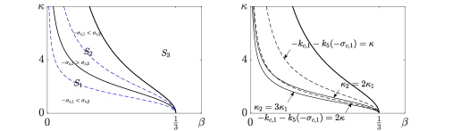
Figure 6. Left panel: In the region bounded by the two blue dash curves, there holds $-\sigma_{c,1}>\sigma_{c,2}$, and in the complement of the former region with respect to the super-critical region there satisfy $-\sigma_{c,1}<\sigma_{c,2}$. Right panel: The region of waves admitting $(k_{1}(\sigma),k_{5}(\sigma),1)\in\mathcal{R}(\sigma)$ for some $\sigma>0$ is bounded from above by the dash curve on which $-k_{c,1}-k_{5}(-\sigma_{c,1})=\kappa$ and below by the solid curve on which $\kappa_{2}=2\kappa_{1}$. The region of waves admitting $(k_{1}(\sigma),k_{5}(\sigma),2)\in\mathcal{R}(\sigma)$ for some $\sigma>0$ is bounded from above by the dash curve on which $-k_{c,1}-k_{5}(-\sigma_{c,1})=2\kappa$ and below by the solid curve on which $\kappa_{2}=3\kappa_{1}$. The region of waves admitting $(k_{6}(\sigma),k_{2}(\sigma),1)\in\mathcal{R}(\sigma)$ for some $\sigma>0$ is bounded from above by the solid curve on which $\kappa_{2}=2\kappa_{1}$. The region of waves admitting $(k_{6}(\sigma),k_{2}(\sigma),2)\in\mathcal{R}(\sigma)$ for some $\sigma>0$ is bounded from above by the solid curve on which $\kappa_{2}=3\kappa_{1}$. The region of waves admitting $(k_{4}(\sigma),k_{5}(\sigma),2)\in\mathcal{R}(\sigma)$ for some $\sigma>0$ is bounded from below by the solid curve on which $\kappa_{2}=2\kappa_{1}$.

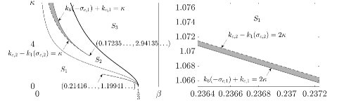
Figure 7. In the $S_{1}$ region, the region of waves admitting $(k_{6}(\sigma),k_{1}(\sigma),2)\in\mathcal{R}(\sigma)$ for some $\sigma>0$ is bounded from above by the dash curve on which $k_{c,2}-k_{1}(\sigma_{c,2})=2\kappa$ and below by the solid curve on which $k_{6}(-\sigma_{c,1})+k_{c,1}=2\kappa$. The dash curve and solid curve intercept at $(0.21416\ldots,1.19941\ldots)$ where $\sigma_{1}=\sigma_{2}$ and $k_{c,1}+k_{c,2}=2\kappa$. See right panel for a blow-up of the dash and solid curves. In the $S_{2}$ region, the region of waves admitting $(k_{6}(\sigma),k_{1}(\sigma),1)\in\mathcal{R}(\sigma)$ for some $\sigma>0$ is bounded from below by the dash curve on which $k_{c,2}-k_{1}(\sigma_{c,2})=\kappa$ and above by the solid curve on which $k_{6}(-\sigma_{c,1})+k_{c,1}=\kappa$. The dash curve and solid curve intercept at $(0.17235\ldots,2.94135\ldots)$ where $\sigma_{1}=\sigma_{2}$ and $k_{c,1}+k_{c,2}=\kappa$.

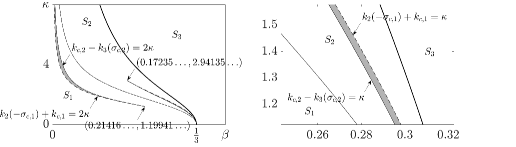
Figure 8. In the $S_{1}$ region, the region of waves admitting $(k_{2}(\sigma),k_{3}(\sigma),2)\in\mathcal{R}(\sigma)$ for some $\sigma>0$ is bounded from above by the solid curve on which $k_{c,2}-k_{3}(\sigma_{c,2})=2\kappa$ and below by the dash curve on which $k_{2}(-\sigma_{c,1})+k_{c,1}=2\kappa$. The dash curve and solid curve intercept at $(0.21416\ldots,1.19941\ldots)$ where $\sigma_{1}=\sigma_{2}$ and $k_{c,1}+k_{c,2}=2\kappa$. In the $S_{2}$ region, the region of waves admitting $(k_{2}(\sigma),k_{3}(\sigma),1)\in\mathcal{R}(\sigma)$ for some $\sigma>0$ is bounded from below by the solid curve on which $k_{c,2}-k_{3}(\sigma_{c,2})=\kappa$ and above by the dash curve on which $k_{2}(-\sigma_{c,1})+k_{c,1}=\kappa$. The dash curve and solid curve intercept at $(0.17235\ldots,2.94135\ldots)$ where $\sigma_{1}=\sigma_{2}$ and $k_{c,1}+k_{c,2}=\kappa$. For a blow-up of the dash and solid curves see right panel.

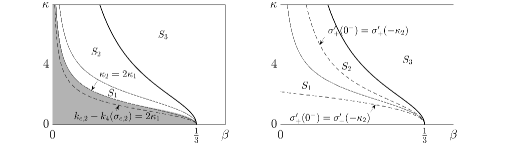
Figure 9. Left panel: The region of waves admitting $(k_{6}(\sigma),k_{4}(\sigma),2)\in\mathcal{R}(\sigma)$ for some $\sigma>0$ is bounded from above by the domain of Wilton ripples of order $2$ and below by the dash curve on which $k_{c,2}-k_{4}(\sigma_{c,2})=2\kappa_{1}$. The region of waves admitting $(k_{2}(\sigma),k_{4}(\sigma),2)\in\mathcal{R}(\sigma)$ for some $\sigma>0$ is bounded from above by the dash curve on which $k_{c,2}-k_{4}(\sigma_{c,2})=2\kappa_{1}$. Right panel: There is a dash curve in the $S_{1}$ region on which $\sigma_{+}^{\prime}(0^{-})=\sigma_{+}^{\prime}(-\kappa_{2})$ and a dash curve in the $S_{2}$ region on which $\sigma_{+}^{\prime}(0^{-})=\sigma_{+}^{\prime}(-\kappa_{2})$. For waves between the two dash curves, $(k_{3}-k_{5})(\sigma)$ is first increasing then decreasing. For waves above the upper dash curve and in the $S_{2}$ region and waves below the lower dash curve and in the $S_{1}$ region, $(k_{3}-k_{5})(\sigma)$ is strictly decreasing.

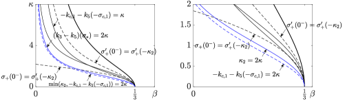
Figure 10. The region of waves admitting

$$(k_{3}(\sigma),k_{5}(\sigma),1)\in\mathcal{R}(\sigma)$$

for some $\sigma>0$ is bounded from above by the upper dash black curve on which $\sigma_{+}^{\prime}(0^{-})=\sigma_{+}^{\prime}(-\kappa_{2})$ and below by the solid black curve on which $-k_{c,1}-k_{5}(-\sigma_{c,1})=\kappa$. These wave are not necessarily all $\kappa_{2}$-waves for clearly in the right panel we see the solid black curve cross the boundary separating $\kappa_{1}$- and $\kappa_{2}$- waves. In the $S_{1}$ region, we find waves admitting $(k_{3}(\sigma),k_{5}(\sigma),2)\in\mathcal{R}(\sigma)$ for some $\sigma>0$. In the region where $(k_{3}-k_{5})(\sigma)$ is first increasing and then decreasing, the region of the waves is bounded from above by the solid blue curve on which $(k_{3}-k_{5})(\sigma_{*})=2\kappa_{1}$ ($\sigma_{*}$ is the critical point for $(k_{3}-k_{5})(\sigma)$, $0<\sigma_{*}<-\sigma_{c,1}$) and below by the dash blue curve on which $\min(\kappa_{2},-k_{c,1}-k_{5}(-\sigma_{c,1}))=2\kappa$. On the right panel, we show, in the region where $(k_{3}-k_{5})(\sigma)$ is strictly decreasing, the region of the waves is bounded from above by the solid blue curve on which $\kappa_{2}=2\kappa_{1}$ and below by the dash blue curve on which $-k_{c,1}-k_{5}(-\sigma_{c,1})=2\kappa$.

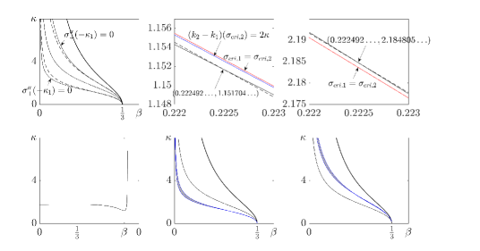
Figure 11. There are two solid curves on which $\sigma_{+}^{\prime\prime}(-\kappa_{1})=0$. See top left panel. One curve is in the $S_{1}$ region and crosses the $-\sigma_{c,1}=\sigma_{c,2}$ dash curve at $(0.222492\ldots,1.151704\ldots)$. See top middle panel. The other one is in the $S_{2}$ region and crosses the $-\sigma_{c,1}=\sigma_{c,2}$ dash curve at $(0.222492\ldots,2.184805\ldots)$. See top right panel. For waves between these two solid curve, $\sigma_{+}^{\prime\prime}(-\kappa_{1})>0$ and hence, $(k_{2}-k_{1})(\sigma)$ is increasing for small $\sigma>0$. In the $S_{1}$ region, for waves that are between the dash $-\sigma_{c,1}=\sigma_{c,2}$ curve and solid $\sigma_{+}^{\prime\prime}(-\kappa_{1})=0$ curve, $(k_{2}-k_{1})(\sigma)$ is first increasing then decreasing for $\beta<0.222492\ldots$ and first decreasing then increasing for $\beta>0.222492\ldots$. Above both the dash curve and the solid $\sigma_{+}^{\prime\prime}(-\kappa_{1})=0$ curve is a region where $(k_{2}-k_{1})(\sigma)$ is first increasing then decreasing and then increasing. A typical $(k_{2}-k_{1})(\sigma)$ versus $\sigma$ graph is shown in the bottom left panel. For waves in this region, $(k_{2}-k_{1})(\sigma)$ is increasing for $0<\sigma<\sigma_{cri,1}$ then decreasing for $\sigma_{cri,1}<\sigma<\sigma_{cri,2}$ and then increasing for $\sigma_{cri,2}<\sigma<\sigma_{c,2}$. Such region is bounded from above by a red curve on which $\sigma_{cri,1}=\sigma_{cri,2}$. See top middle panel. In the $S_{2}$ region, for waves that are between the dash $-\sigma_{c,1}=\sigma_{c,2}$ curve and solid $\sigma_{+}^{\prime\prime}(-\kappa_{1})=0$ curve, $(k_{2}-k_{1})(\sigma)$ is first increasing then decreasing for $\beta<0.222492\ldots$ and first decreasing then increasing for $\beta>0.222492\ldots$. Below both the dash curve and the solid $\sigma_{+}^{\prime\prime}(-\kappa_{1})=0$ curve, again, is a region where $(k_{2}-k_{1})(\sigma)$ is first increasing then decreasing and then increasing. Such region is bounded from below by a red curve on which $\sigma_{cri,1}=\sigma_{cri,2}$. See top right panel.

Figure 11. (Previous page.) Based on the monotonicity of $(k_{2}-k_{1})(\sigma)$, we find, in the $S_{1}$ region, the region of waves admitting $(k_{2}-k_{1})(\sigma)=2\kappa$ is bounded from above and below by two blue boundary curves shown in the bottom middle panel. The upper boundary crosses the dash curve $-\sigma_{c,1}=\sigma_{c,2}$ from left to right when $\beta$ increases and passes $0.214164\ldots$. For $\beta<0.214164\ldots$, the curve is given by tracing $k_{2}(-\sigma_{c,1})+k_{c,1}=2\kappa$ and, for $\beta>0.214164\ldots$, the curve is given by tracing $(k_{2}-k_{1})(\sigma_{cri,2})=2\kappa$. The lower boundary curve is given by the part of solid $\sigma_{+}^{\prime\prime}(-\kappa_{1})=0$ curve with $\beta<0.222603\ldots$ and given by tracing $k_{c,2}-k_{1}(\sigma_{c,2})=2\kappa$ for $\beta>0.222603\ldots$. In the $S_{2}$ region, the region of waves admitting $(k_{2}-k_{1})(\sigma)=\kappa$ is bounded from above and below by two blue boundary curves shown in the bottom right panel. We omit details on how we trace these two boundaries.

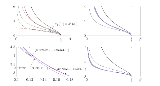
Figure 12. There are two curves on which $\sigma_{+}^{\prime}(0^{-})=\sigma_{-}^{\prime}(\kappa_{2})$. See top left panel. One is in the $S_{1}$ region and the other one is in the $S_{2}$ region. For waves between these two solid curve, $\sigma_{+}^{\prime}(0^{-})-\sigma_{-}^{\prime}(\kappa_{2})<0$ and hence, $(k_{6}-k_{3})(\sigma)$ is decreasing for small $\sigma>0$. In the $S_{2}$ region, for waves that are between the dash $-\sigma_{c,1}=\sigma_{c,2}$ curve and solid $\sigma_{+}^{\prime}(0^{-})=\sigma_{-}^{\prime}(\kappa_{2})$ curve, $(k_{6}-k_{3})(\sigma)$ is first decreasing then increasing for $\beta<0.127595\ldots$ and first increasing then decreasing for $\beta>0.127595\ldots$. Above both the dash curve and the solid $\sigma_{+}^{\prime}(0^{-})=\sigma_{-}^{\prime}(\kappa_{2})$ curve is a region where $(k_{6}-k_{3})(\sigma)$ is first increasing then decreasing and then increasing. For waves in this region, $(k_{6}-k_{3})(\sigma)$ is increasing for $0<\sigma<\sigma_{cri,1}$ then decreasing for $\sigma_{cri,1}<\sigma<\sigma_{cri,2}$ and then increasing for $\sigma_{cri,2}<\sigma<\sigma_{c,1}$. Such region is bounded from above by a red curve on which $\sigma_{cri,1}=\sigma_{cri,2}$. In the $S_{1}$ region, below both the dash $-\sigma_{c,1}=\sigma_{c,2}$ curve and the solid $\sigma_{+}^{\prime}(0^{-})=\sigma_{-}^{\prime}(\kappa_{2})$ curve, again, is a region where $(k_{6}-k_{3})(\sigma)$ is first increasing then decreasing and then increasing. Such region is bounded from below by a red curve on which $\sigma_{cri,1}=\sigma_{cri,2}$. Based on the monotonicity of $(k_{6}-k_{3})(\sigma)$, we find, in the $S_{2}$ region, the region of waves admitting $(k_{6}-k_{3})(\sigma)=\kappa$ is bounded from above and below by two blue boundary curves shown in the top right panel. The upper boundary crosses the $-\sigma_{c,1}=\sigma_{c,2}$ dash curve from left to right when $\beta$ increases and passes $0.172350\ldots$. For $\beta<0.172350\ldots$, the curve is given by tracing $(k_{6}-k_{3})(\sigma_{cri,2})=\kappa$ and, for $\beta>0.172350\ldots$, the curve is given by tracing $k_{c,2}-k_{3}(\sigma_{cri,2})=\kappa$.

Figure 12. (Previous page.) The lower boundary curve is given by the part of solid $\sigma_{+}^{\prime}(0^{-})=\sigma_{-}^{\prime}(\kappa_{2})$ curve with $\beta>0.122892\ldots$ and given by tracing $k_{6}(-\sigma_{c,1})+k_{c,1}=\kappa$ for $\beta<0.172350\ldots$. In the $S_{1}$ region, the region of waves admitting $(k_{6}-k_{3})(\sigma)=2\kappa$ is bounded from above and below by two blue boundary curves shown in the bottom right panel. We omit details on how we trace these two boundaries.

We note, as we will see from below, that the critical frequencies $-i\sigma_{c,1},i\sigma_{c,2}$ can be resonant frequencies, which does not happen for Stokes waves [17].

• Waves admitting $(k_{1}(\sigma),k_{5}(\sigma),N)\in\mathcal{R}(\sigma)$ for $N=1$ ($N=2$) and some $\sigma>0$. Because $(k_{1}-k_{5})(\sigma)$ is strictly increasing and we find $\kappa_{2}-\kappa_{1}<(k_{1}-k_{5})(\sigma)<-k_{c,1}-k_{5}(-\sigma_{c,1})$ for $\sigma>0$, the region of these waves is bounded from below by the domain of Wilton ripples of order 2 (order 3) and above by a curve satisfying $-k_{c,1}-k_{5}(-\sigma_{c,1})=\kappa$ $\big{(}-k_{c,1}-k_{5}(-\sigma_{c,1})=2\kappa\big{)}$. See FIGURE 6 right panel.

• Waves admitting $(k_{6}(\sigma),k_{2}(\sigma),N)\in\mathcal{R}(\sigma)$ for $N=1$ ($N=2$) and some $\sigma>0$. Because $(k_{6}-k_{2})(\sigma)$ is strictly decreasing and we find $0\leqslant(k_{6}-k_{2})(\sigma)<\kappa_{2}-\kappa_{1}$ for $\sigma>0$, the region of these waves is bounded from above by the domain of Wilton ripples of order 2 (order 3). See FIGURE 6 right panel.

• There is no $\sigma>0$ such that $(k_{2}(\sigma),k_{5}(\sigma),N)\in\mathcal{R}(\sigma)$ for $N=1$ or $2$. This is because $(k_{2}-k_{5})(\sigma)$ is strictly increasing and $2\kappa_{1}<\kappa_{1}+\kappa_{2}<(k_{2}-k_{5})(\sigma)\leqslant k_{c,2}-k_{5}(\sigma_{c,2})<2\kappa_{2}$ for $\sigma>0$. Here the last inequality is obtained from Lemma 4.6[i].

• Waves admitting $(k_{4}(\sigma),k_{5}(\sigma),2)\in\mathcal{R}(\sigma)$ for some $\sigma>0$. Because $(k_{4}-k_{5})(\sigma)>\kappa_{2}$ is strictly increasing and unbounded, the region of these waves is bounded from below by the domain of Wilton ripples of order 2. See FIGURE 6 right panel.

• There is no $\sigma>0$ such that $(k_{3}(\sigma),k_{1}(\sigma),N)\in\mathcal{R}(\sigma)$ for $N=1$ or $2$. This is because $(k_{3}-k_{1})(\sigma)$ is strictly decreasing and we find $0\leqslant(k_{3}-k_{1})(\sigma)<\kappa_{1}<\kappa_{2}$ for $\sigma>0$.

• Waves admitting $(k_{6}(\sigma),k_{1}(\sigma),N)\in\mathcal{R}(\sigma)$ for $N=1$ ($N=2$) and some $\sigma>0$. Because $(k_{6}-k_{1})(\sigma)$ is strictly decreasing, we find, if $-\sigma_{c,1}\leqslant\sigma_{c,2}$, then $\kappa_{1}<k_{6}(-\sigma_{c,1})+k_{c,1}\leqslant(k_{6}-k_{1})(\sigma)<\kappa_{1}+\kappa_{2}<2\kappa_{2}$, and if $-\sigma_{c,1}>\sigma_{c,2}$, then $\kappa_{1}<k_{c,2}-k_{1}(\sigma_{c,2})\leqslant(k_{6}-k_{1})(\sigma)<\kappa_{1}+\kappa_{2}<2\kappa_{2}$. Therefore, in $S_{1}$ region, the region of waves admitting $(k_{6}(\sigma),k_{1}(\sigma),2)\in\mathcal{R}(\sigma)$ for some $\sigma>0$ is bounded by a curve satisfying $k_{6}(-\sigma_{c,1})+k_{c,1}=2\kappa_{1}$ in the $-\sigma_{c,1}<\sigma_{c_{2}}$ region and a curve satisfying $k_{c,2}-k_{1}(\sigma_{c,2})=2\kappa_{1}$ in the $-\sigma_{c,1}>\sigma_{c_{2}}$ region. In the $S_{2}$ region, the region of waves admitting $(k_{6}(\sigma),k_{1}(\sigma),1)\in\mathcal{R}(\sigma)$ for some $\sigma>0$ is bounded by a curve satisfying $k_{6}(-\sigma_{c,1})+k_{c,1}=\kappa_{2}$ in the $-\sigma_{c,1}<\sigma_{c,2}$ region and a curve satisfying $k_{c,2}-k_{1}(\sigma_{c,2})=\kappa_{2}$ in the $-\sigma_{c,1}>\sigma_{c,2}$ region. See FIGURE 7.

• Waves admitting $(k_{2}(\sigma),k_{3}(\sigma),N)\in\mathcal{R}(\sigma)$ for $N=1$ ($N=2$) and some $\sigma>0$. Because $(k_{2}-k_{3})(\sigma)$ is strictly increasing, we find, if $-\sigma_{c,1}\leqslant\sigma_{c,2}$, then $\kappa_{1}<(k_{2}-k_{3})(\sigma)\leqslant k_{2}(-\sigma_{c,1})+k_{c,1}\leqslant k_{6}(-\sigma_{c,1})+k_{c,1}<\kappa_{1}+\kappa_{2}<2\kappa_{2}$, and if $-\sigma_{c,1}>\sigma_{c,2}$, then $\kappa_{1}<(k_{2}-k_{3})(\sigma)\leqslant k_{c,2}-k_{3}(\sigma_{c,2})<k_{c,2}-k_{1}(\sigma_{c,2})<\kappa_{1}+\kappa_{2}<2\kappa_{2}$. Therefore, in $S_{1}$ region, the region of waves admitting $(k_{2}(\sigma),k_{3}(\sigma),2)\in\mathcal{R}(\sigma)$ for some $\sigma>0$ is bounded by a curve satisfying $k_{2}(-\sigma_{c,1})+k_{c,1}=2\kappa_{1}$ in the $-\sigma_{c,1}<\sigma_{c_{2}}$ region and a curve satisfying $k_{c,2}-k_{3}(\sigma_{c,2})=2\kappa_{1}$ in the $-\sigma_{c,1}>\sigma_{c,2}$ region. In the $S_{2}$ region, the region of waves admitting $(k_{2}(\sigma),k_{3}(\sigma),1)\in\mathcal{R}(\sigma)$ for some $\sigma>0$ is bounded by a curve satisfying $k_{2}(-\sigma_{c,1})+k_{c,1}=\kappa_{2}$ in the $-\sigma_{c,1}<\sigma_{c,2}$ region and a curve satisfying $k_{c,2}-k_{3}(\sigma_{c,2})=\kappa_{2}$ in the $-\sigma_{c,1}>\sigma_{c,2}$ region. See FIGURE 8.

• There is no $\sigma>0$ such that $(k_{4}(\sigma),k_{3}(\sigma),N)\in\mathcal{R}(\sigma)$ for $N=1$ or $2$. This is because $(k_{4}-k_{3})(\sigma)$ is strictly increasing and we find $0<(k_{4}-k_{3})(\sigma)<k_{4}(-\sigma_{c,1})+k_{c,1}$ and $k_{4}(-\sigma_{c,1})+k_{c,1}<\kappa_{1}$. Here the last inequality is obtained from Lemma 4.6[ii].

• Waves admitting $(k_{6}(\sigma),k_{4}(\sigma),2)\in\mathcal{R}(\sigma)$ for some $\sigma>0$. Recall Lemma 4.6[iii], $(k_{2}-k_{4})(\sigma)$ is strictly increasing for $\sigma\in(0,\sigma_{c,2}]$. We find $\kappa_{1}<k_{c,2}-k_{4}(\sigma_{c,2})\leqslant(k_{6}-k_{4})(\sigma)<\kappa_{2}$. In the $S_{1}$ region, the region of waves admitting $(k_{6}(\sigma),k_{4}(\sigma),2)\in\mathcal{R}(\sigma)$ for some $\sigma>0$ is bounded from above by the domain of Wilton ripples of order 2 and below by a curve satisfying $k_{c,2}-k_{4}(\sigma_{c,2})=2\kappa_{1}$. See FIGURE 9 left panel.

• There is no $\sigma>0$ such that $(k_{6}(\sigma),k_{5}(\sigma),N)\in\mathcal{R}(\sigma)$ for $N=1$ or $2$. Recall Lemma 4.6[i] $(k_{6}-k_{5})(\sigma)$ is strictly decreasing on $(0,\sigma_{c,2}]$ and $2\kappa_{1}<\kappa_{1}+\kappa_{2}<k_{c,2}-k_{5}(\sigma_{c,2})<(k_{6}-k_{5})(\sigma)<2\kappa_{2}$ for $\sigma>0$.

• There is no $\sigma>0$ such that $(k_{4}(\sigma),k_{1}(\sigma),N)\in\mathcal{R}(\sigma)$ for $N=1$ or $2$. Recall Lemma 4.6[ii] $(k_{4}-k_{1})(\sigma)$ is strictly decreasing on $(0,-\sigma_{c,1}]$ and $(k_{4}-k_{1})(\sigma)<\kappa_{1}$ for $\sigma>0$.

• Waves admitting $(k_{2}(\sigma),k_{4}(\sigma),2)\in\mathcal{R}(\sigma)$. Recall Lemma 4.6[iii] $(k_{4}-k_{2})(\sigma)$ is strictly increasing on $(0,\sigma_{c,2}]$ and $\kappa_{1}<(k_{2}-k_{4})(\sigma)<k_{c,2}-k_{4}(\sigma_{c,2})<\kappa_{2}$ for $\sigma>0$. So in the $S_{1}$ region, there are waves admitting $(k_{2}(\sigma),k_{4}(\sigma),2)\in\mathcal{R}(\sigma)$ which are bounded from above by a curve satisfying $k_{c,2}-k_{4}(\sigma_{c,2})=2\kappa_{1}$. See FIGURE 9 left panel.

The difference $(k_{3}-k_{5})(\sigma)$ may not be monotonic. Recall from Lemma 3.4, $\sigma_{-}(\cdot;\beta,\mu_{0})$ is convex on $[0,k_{*})$ and concave on $(k_{*},\infty)$ for a $k_{*}\in(k_{c,1},k_{c,2})$. Further analyses show the following lemma holds.

Lemma 4.7.

If $\sigma_{+}^{\prime}(0^{-};\beta,\mu_{0})<\sigma_{+}^{\prime}(-\kappa_{2};\beta.\mu_{0})$, then, for $\sigma\in[0,-\sigma_{c,1}]$, $(k_{3}-k_{5})(\sigma)$ is first increasing then decreasing, otherwise, $(k_{3}-k_{5})(\sigma)$ is strictly decreasing.

Proof.

For $\sigma\in[0,-\sigma_{c,1}]$, $\sigma_{+}^{\prime}(k_{5}(\sigma)),\sigma_{+}^{\prime}(k_{3}(\sigma))<0$. The sign of $(k_{3}-k_{5})^{\prime}(\sigma)=\frac{\sigma_{+}^{\prime}(k_{5}(\sigma))-\sigma_{+}^{\prime}(k_{3}(\sigma))}{\sigma_{+}^{\prime}(k_{5}(\sigma))\sigma_{+}^{\prime}(k_{3}(\sigma))}$ is given by that of $\sigma_{+}^{\prime}(k_{5}(\sigma))-\sigma_{+}^{\prime}(k_{3}(\sigma))$. Recall from Lemma 3.4, $\sigma_{+}^{\prime\prime}(k_{5}(\sigma))=-\sigma_{-}^{\prime\prime}(k_{6}(-\sigma))>0$ and $\sigma_{+}^{\prime\prime}(k_{3}(\sigma))=\sigma_{-}^{\prime\prime}(k_{2}(-\sigma))<0$, $\sigma_{+}^{\prime\prime}(k_{5}(\sigma))k_{5}^{\prime}(\sigma)-\sigma_{+}^{\prime\prime}(k_{3}(\sigma))k_{3}^{\prime}(\sigma)<0$. Hence $\sigma_{+}^{\prime}(k_{5}(\sigma))-\sigma_{+}^{\prime}(k_{3}(\sigma))$ is decreasing for $\sigma\in[0,-\sigma_{c,1}]$. We compute $\sigma_{+}^{\prime}(k_{5}(-\sigma_{c,1}))-\sigma_{+}^{\prime}(-k_{c,1})=\sigma_{+}^{\prime}(k_{5}(-\sigma_{c,1}))<0$, which completes the proof. ∎

• Waves admitting $(k_{3}(\sigma),k_{5}(\sigma),N)\in\mathcal{R}(\sigma)$ for $N=1$ ($N=2$) and some $\sigma>0$. Recall Lemma 4.7, we investigate curves on which $\sigma_{+}^{\prime}(0^{-})=\sigma_{+}^{\prime}(-\kappa_{2})$. See FIGURE 9 right panel. Based Lemma 4.7, we find that the region of waves admitting $(k_{3}(\sigma),k_{5}(\sigma),1)\in\mathcal{R}(\sigma)$ for some $\sigma>0$ is bounded from above by a curve satisfying $\sigma_{+}^{\prime}(0^{-})=\sigma_{+}^{\prime}(-\kappa_{2})$ and below by a curve satisfying $-k_{c,1}-k_{5}(-\sigma_{c,1})=\kappa$. In the $S_{1}$ region, we find waves admitting $(k_{3}(\sigma),k_{5}(\sigma),2)\in\mathcal{R}(\sigma)$ and some $\sigma>0$. In the region where $(k_{3}-k_{5})(\sigma)$ is first increasing then decreasing and achieves its maximum at $\sigma_{*}$, the region of the waves is then bounded from above by a curve on which $(k_{3}-k_{5})(\sigma_{*})=2\kappa$ and below by a curve on which $\min(\kappa_{2},-k_{c,1}-k_{5}(-\sigma_{c,1}))=2\kappa$. In the region where $(k_{3}-k_{5})(\sigma)$ is always decreasing, the region of the waves is bounded from above by the domain of Wilton ripples of order 2 and below by a curve on which $-k_{c,1}-k_{5}(-\sigma_{c,1})=2\kappa$. See FIGURE 10.

As analyzed below, more complicated are the behaviors of differences $(k_{2}-k_{1})(\sigma)$ and $(k_{6}-k_{3})(\sigma)$.

• Waves admitting $(k_{2}(\sigma),k_{1}(\sigma),N)\in\mathcal{R}(\sigma)$ for $N=1$ ($N=2$) and some $\sigma>0$. For $\sigma\in(0,\min(-\sigma_{c,1},\sigma_{c,2}))$, $\sigma_{+}^{\prime}(k_{1}(\sigma)),\sigma_{-}^{\prime}(k_{2}(\sigma))>0$. The sign of $(k_{2}-k_{1})^{\prime}(\sigma)=\frac{\sigma_{+}^{\prime}(k_{1}(\sigma))-\sigma_{-}^{\prime}(k_{2}(\sigma))}{\sigma_{+}^{\prime}(k_{1}(\sigma))\sigma_{-}^{\prime}(k_{2}(\sigma))}$ is given by that of $\sigma_{+}^{\prime}(k_{1}(\sigma))-\sigma_{-}^{\prime}(k_{2}(\sigma))$. In the $-\sigma_{c,1}>\sigma_{c,2}$ region, $\sigma_{+}^{\prime}(k_{1}(\sigma_{c,2}))-\sigma_{-}^{\prime}(k_{c,2})=\sigma_{+}^{\prime}(k_{1}(\sigma_{c,2}))>0$, so $(k_{2}-k_{1})(\sigma)$ is increasing for sufficiently large $\sigma$. In the $-\sigma_{c,1}<\sigma_{c,2}$ region, $\sigma_{+}^{\prime}(-k_{c,1})-\sigma_{-}^{\prime}(k_{2}(-\sigma_{c,1}))=-\sigma_{-}^{\prime}(k_{2}(-\sigma_{c,1}))<0$, so $(k_{2}-k_{1})(\sigma)$ is decreasing for sufficiently large $\sigma$. For small $\sigma>0$, because $\sigma_{+}^{\prime}(k_{1}(0))-\sigma_{-}^{\prime}(k_{2}(0))=0$, the sign of $(k_{2}-k_{1})^{\prime}(\sigma)$ is given by $\mathrm{sgn}(\sigma_{+}^{\prime\prime}(k_{1}(0))k_{1}^{\prime}(0)-\sigma_{-}^{\prime\prime}(k_{2}(0))k_{2}^{\prime}(0))=\mathrm{sgn}(\sigma_{+}^{\prime\prime}(-\kappa_{1})k_{1}^{\prime}(0))=\mathrm{sgn}(\sigma_{+}^{\prime\prime}(-\kappa_{1}))$. We then trace the curves satisfying $\sigma_{+}^{\prime\prime}(-\kappa_{1})=0$. Above the lower boundary of the $-\sigma_{c,1}>\sigma_{c,2}$ region and the lower curve on which $\sigma_{+}^{\prime\prime}(-\kappa_{1})=0$, we find a region where $(k_{2}-k_{1})(\sigma)$ is first increasing then decreasing and then increasing. Such region is bounded from above by a curve on which there is exactly one critical point of $(k_{2}-k_{1})(\sigma)$ for $0\leqslant\sigma<\sigma_{c,2}$. Below the upper boundary of the $-\sigma_{c,1}>\sigma_{c,2}$ region and the upper curve on which $\sigma_{+}^{\prime\prime}(-\kappa_{1})=0$, we find a region where $(k_{2}-k_{1})(\sigma)$ is first increasing then decreasing and then increasing. Such region is bounded from above by a curve on which there is exactly one critical point of $(k_{2}-k_{1})(\sigma)$ for $0\leqslant\sigma<\sigma_{c,2}$. Based on the monotonicity of $(k_{2}-k_{1})(\sigma)$, we find waves admitting $(k_{2}(\sigma),k_{1}(\sigma),2)\in\mathcal{R}(\sigma)$ for some $\sigma>0$ in the $S_{1}$ region and waves admitting $(k_{2}(\sigma),k_{1}(\sigma),1)\in\mathcal{R}(\sigma)$ for some $\sigma>0$ in the $S_{2}$ region. See FIGURE 11.

• Waves admitting $(k_{6}(\sigma),k_{3}(\sigma),N)\in\mathcal{R}(\sigma)$ for $N=1$ ($N=2$) and some $\sigma>0$. For $\sigma\in(0,\min(-\sigma_{c,1},\sigma_{c,2}))$, $\sigma_{+}^{\prime}(k_{3}(\sigma)),\sigma_{-}^{\prime}(k_{6}(\sigma))<0$. The sign of $(k_{6}-k_{3})^{\prime}(\sigma)=\frac{\sigma_{+}^{\prime}(k_{3}(\sigma))-\sigma_{-}^{\prime}(k_{6}(\sigma))}{\sigma_{+}^{\prime}(k_{3}(\sigma))\sigma_{-}^{\prime}(k_{6}(\sigma))}$ is given by that of $\sigma_{+}^{\prime}(k_{3}(\sigma))-\sigma_{-}^{\prime}(k_{6}(\sigma))$. In the $-\sigma_{c,1}>\sigma_{c,2}$ region, $\sigma_{+}^{\prime}(k_{3}(\sigma_{c,2}))-\sigma_{-}^{\prime}(k_{c,2})=\sigma_{+}^{\prime}(k_{3}(\sigma_{c,2}))<0$, so $(k_{6}-k_{3})(\sigma)$ is decreasing for sufficiently large $\sigma$. In the $-\sigma_{c,1}<\sigma_{c,2}$ region, $\sigma_{+}^{\prime}(-k_{c,1})-\sigma_{-}^{\prime}(k_{6}(-\sigma_{c,1}))=-\sigma_{-}^{\prime}(k_{6}(-\sigma_{c,1}))>0$, so $(k_{6}-k_{3})(\sigma)$ is increasing for sufficiently large $\sigma$. For small $\sigma>0$, the monotonicity of $(k_{6}-k_{3})(\sigma)$ is ruled by the sign of $\sigma_{+}^{\prime}(0^{-})-\sigma_{-}^{\prime}(\kappa_{2})$. We then trace the curves on which $\sigma_{+}^{\prime}(0^{-})=\sigma_{-}^{\prime}(\kappa_{2})$. In the upper $-\sigma_{c,1}<\sigma_{c,2}$ region and above the curve on which $\sigma_{+}^{\prime}(0^{-})=\sigma_{-}^{\prime}(\kappa_{2})$, we find a region where $(k_{6}-k_{3})(\sigma)$ is first increasing then decreasing and then increasing. Such region is bounded from above by a curve on which there is exactly one critical point of $(k_{6}-k_{3})(\sigma)$ for $0\leqslant\sigma<-\sigma_{c,1}$. In the lower $-\sigma_{c,1}<\sigma_{c,2}$ region and below the curve on which $\sigma_{+}^{\prime}(0^{-})=\sigma_{-}^{\prime}(\kappa_{2})$, we find a region where $(k_{6}-k_{3})(\sigma)$ is first increasing then decreasing and then increasing. Such region is bounded from above by a curve on which there is exactly one critical point of $(k_{6}-k_{3})(\sigma)$ for $0\leqslant\sigma<-\sigma_{c,1}$. Based on the monotonicity of $(k_{6}-k_{3})(\sigma)$, we find waves admitting $(k_{6}(\sigma),k_{3}(\sigma),N)\in\mathcal{R}(\sigma)$ for $N=1$ ($N=2$) and some $\sigma>0$ and we trace the boundaries of these waves as shown in FIGURE 12.

There can be waves admit two pairs of resonant eigenvalues at the critical frequencies $-i\sigma_{c,1}$ or $i\sigma_{c,2}$. For example, for waves on the curve satisfying $-k_{c,1}-k_{5}(-\sigma_{c,1})=2\kappa$ (see FIGURE 6 right panel) because $-k_{c,1}=k_{1}(-\sigma_{c,1})=k_{3}(-\sigma_{c,1})$ hence

$$(k_{1}(-\sigma_{c,1}),k_{5}(-\sigma_{c,1}),2),\quad(k_{3}(-\sigma_{c,1}),k_{5}(-\sigma_{c,1}),2)\in\mathcal{R}(-\sigma_{c,1}).$$

Similarly,

• On the curve satisfying $-k_{c,1}-k_{5}(-\sigma_{c,1})=N\kappa$, $N=1$ or $2$ (see FIGURE 6 right panel), waves admit

  $$(k_{1}(-\sigma_{c,1}),k_{5}(-\sigma_{c,1}),N),\quad(k_{3}(-\sigma_{c,1}),k_{5}(-\sigma_{c,1}),N)\in\mathcal{R}(-\sigma_{c,1});$$

• On the curve satisfying $k_{6}(-\sigma_{c,1})+k_{c,1}=N\kappa$, $N=1$ or $2$ (see FIGURE 7), waves admit $(k_{6}(-\sigma_{c,1}),k_{1}(-\sigma_{c,1}),N),(k_{6}(-\sigma_{c,1}),k_{3}(-\sigma_{c,1}),N)\in\mathcal{R}(-\sigma_{c,1})$;
  On the curve satisfying $k_{c,2}-k_{1}(\sigma_{c,2})=N\kappa$, $N=1$ or $2$ (see FIGURE 7), waves admit $(k_{2}(\sigma_{c,2}),k_{1}(\sigma_{c,2}),N),(k_{6}(\sigma_{c,2}),k_{1}(\sigma_{c,2}),N)\in\mathcal{R}(\sigma_{c,2})$;

• On the curve satisfying $k_{2}(-\sigma_{c,1})+k_{c,1}=N\kappa$, $N=1$ or $2$ (see FIGURE 8), waves admit $(k_{2}(-\sigma_{c,1}),k_{1}(-\sigma_{c,1}),N),(k_{2}(-\sigma_{c,1}),k_{3}(-\sigma_{c,1}),N)\in\mathcal{R}(-\sigma_{c,1})$;
  On the curve satisfying $k_{c,2}-k_{3}(\sigma_{c,2})=N\kappa$, $N=1$ or $2$ (see FIGURE 8), waves admit $(k_{2}(\sigma_{c,2}),k_{3}(\sigma_{c,2}),N),(k_{6}(\sigma_{c,2}),k_{3}(\sigma_{c,2}),N)\in\mathcal{R}(\sigma_{c,2})$;

• On the curve satisfying $k_{c,2}-k_{4}(\sigma_{c,2})=2\kappa$, (see FIGURE 9 left panel), waves admit $(k_{2}(\sigma_{c,2}),k_{4}(\sigma_{c,2}),2),(k_{6}(\sigma_{c,2}),k_{4}(\sigma_{c,2}),2)\in\mathcal{R}(\sigma_{c,2})$.

5. Spectral instability of non-resonant capillary-gravity waves

5.1. The spectrum away from the origin

For a $(\beta,\kappa)$-wave, if $i\sigma$, $\sigma>0$ is a resonant frequency, let $(k_{j},k_{j^{\prime}},N)\in\mathcal{R}(\sigma)$. By Theorem 4.5, we expand the periodic Evans function (3.9) near the root $(i\sigma,k_{j}+p\kappa;0)$ where $i\sigma$ is a resonant frequency and compute the corresponding Weierstrass polynomial, see (LABEL:general_expansion)–(4.4), to detect possible instability. Completion of the task relies on the expansion of the fundamental solution $\mathbf{X}(T;\sigma,\delta,\varepsilon)$ (3.50) as outlined in Section 3.6. The fundamental solution could be a $6$ by $6$ matrix when $0<\sigma<\min\{-\sigma_{c,1},\sigma_{c,2}\}$, a $4$ by $4$ matrix when $\min\{-\sigma_{c,1},\sigma_{c,2}\}<\sigma<\max\{-\sigma_{c,1},\sigma_{c,2}\}$, or a $2$ by $2$ matrix when $\max\{-\sigma_{c,1},\sigma_{c,2}\}<\sigma$. Because, as shown in Section 4, there are a number of resonance cases, it is impossible for us to visit every one of them in the write-up. However, we will demonstrate how computations are carried out for several typical cases.

5.1.1. Resonant frequencies with $N=1$

In contrast to Stokes waves [17] which admit no pair of $1$-resonant eigenvalues at any frequency $i\sigma\in i\mathbb{R}$, in Section 4.2, we see there are waves in the super-critical region that admit pairs of $1$-resonant eigenvalues for some $i\sigma\in i\mathbb{R}$, i.e., $(k_{j}(\sigma),k_{j^{\prime}}(\sigma),1)\in\mathcal{R}(\sigma)$. We therefore deal with these waves first and make the expansion of the Evans function near $(i\sigma,k_{j}+p\kappa;0)$. The dimension of $Y(\sigma)$ can be either $4$ or $6$, and hence $\mathbf{a}^{(m,n)}$ are either $4$ by $4$ matrices or $6$ by $6$ matrices. In either case, there holds the following lemma.

Lemma 5.1.

For waves admitting $(k_{j}(\sigma),k_{j^{\prime}}(\sigma),1)\in\mathcal{R}(\sigma)$, for convenience, we switch the position of resonant modes $\boldsymbol{\phi}_{j}$ and $\boldsymbol{\phi}_{j^{\prime}}$ with the first two modes in the basis $\mathcal{B}(\sigma)$ so that the resonance happens between the first two modes of $\mathcal{B}(\sigma)$. At the resonant frequency $i\sigma$, the left top $2$ by $2$ block matrix of $\mathbf{a}^{(0,0)}(T)$ reads $e^{ik_{j}T}\begin{pmatrix}1&0\\ 0&1\end{pmatrix}$, the off-diagonal entries of the left top $2$ by $2$ block matrix of $\mathbf{a}^{(1,0)}(T)$ necessarily vanish and the diagonal entries are given in (4.8) with $j$ set to $j$ and $j^{\prime}$, and the diagonal entries of the left top $2$ by $2$ block matrix of $\mathbf{a}^{(0,1)}(T)$ necessarily vanish and the off-diagonal entries do not necessarily vanish.

Proof.

The proof is based on explicit computations of solutions of (3.59). See similar calculations made in [17, Section 6.1 and Lemma 6.3]. In particular, we note from

$$a^{(0,1)}_{12}(T)=e^{ik_{j}T}\left\langle\int_{0}^{T}e^{i(k_{j^{\prime}}-k_{j})x}\mathbf{B}^{(0,1)}(x;\sigma)\boldsymbol{\phi}_{j^{\prime}}dx,\boldsymbol{\psi}_{j}\right\rangle$$

and

$$a^{(0,1)}_{21}(T)=e^{ik_{j^{\prime}}T}\left\langle\int_{0}^{T}e^{i(k_{j}-k_{j^{\prime}})x}\mathbf{B}^{(0,1)}(x;\sigma)\boldsymbol{\phi}_{j}dx,\boldsymbol{\psi}_{j^{\prime}}\right\rangle$$

that the off-diagonal entries $a^{(0,1)}_{12}(T)$ and $a^{(0,1)}_{21}(T)$ do not necessarily vanish because terms containing $e^{\pm i\kappa x}\,{\rm s}(\kappa x)$ and $e^{\pm i\kappa x}\,{\rm c}(\kappa x)$ in the integrand do not vanish after integrating over one period. ∎

For waves admitting $(k_{j}(\sigma),k_{j^{\prime}}(\sigma),1)\in\mathcal{R}(\sigma)$ in the super-critical region and when $Y(\sigma)$ is four dimensional, let $\mathcal{B}(\sigma)=\{\boldsymbol{\phi}_{j},\boldsymbol{\phi}_{j^{\prime}},\boldsymbol{\phi}_{r},\boldsymbol{\phi}_{s}\}$. For the moment, let us assume $k_{r},k_{s}\not\equiv k_{j},k_{j^{\prime}}\pmod{\kappa}$, i.e. the remaining two eigenvalues $k_{r},k_{s}$ are not resonant with $k_{j},k_{j^{\prime}}$. See Lemma 5.16 – Theorem 5.20 for treatment of the case where the assumption does not hold. At the resonant frequency $i\sigma$, the periodic Evans function then expands as

$$\Delta(i\sigma+\delta,k_{j}(\sigma)+p\kappa+\gamma;\varepsilon)$$ (5.1)

$$= d^{(2,0,0)}\delta^{2}+d^{(1,1,0)}\gamma\delta+d^{(0,2,0)}\gamma^{2}+d^{(0,0,2)}\varepsilon^{2}+\mathchoice{{\scriptstyle\mathcal{O}}}{{\scriptstyle\mathcal{O}}}{{\scriptscriptstyle\mathcal{O}}}{\scalebox{0.7}{$\scriptscriptstyle\mathcal{O}$}}(|\delta|+|\gamma|+|\varepsilon|)^{2},$$

where

$$d^{(2,0,0)}= a_{11}^{(1,0)}a_{22}^{(1,0)}(e^{ik_{j}T}-e^{ik_{r}T})(e^{ik_{j}T}-e^{ik_{s}T})\neq 0,$$ (5.2)

$$d^{(1,1,0)}= -iT(a_{11}^{(1,0)}+a_{22}^{(1,0)})e^{ik_{j}T}(e^{ik_{j}T}-e^{ik_{r}T})(e^{ik_{j}T}-e^{ik_{s}T}),$$

$$d^{(0,2,0)}= -T^{2}e^{2ik_{j}T}(e^{ik_{j}T}-e^{ik_{r}T})(e^{ik_{j}T}-e^{ik_{s}T}),$$

$$d^{(0,0,2)}= -a_{12}^{(0,1)}a_{21}^{(0,1)}(e^{ik_{j}T}-e^{ik_{r}T})(e^{ik_{j}T}-e^{ik_{s}T}).$$

Here, we infer from (4.8) and the assumption above that $d^{(2,0,0)}\neq 0$. For the Weierstrass’s factorization $\Delta(i\sigma+\delta,k_{j}(\sigma)+p\kappa+\gamma;\varepsilon)=W(\delta,\gamma,\varepsilon)h(\delta,\gamma,\varepsilon)$ (4.3), computation reveals that (4.4) reads

$$W(\delta,\gamma,\varepsilon) =\delta^{2}+a_{1}(\gamma,\varepsilon)\delta+a_{0}(\gamma,\varepsilon),\quad\text{where}$$ (5.3)

$$a_{1}(\gamma,\varepsilon) =d^{(1,1,0)}\big{(}d^{(2,0,0)}\big{)}^{-1}\gamma+\mathchoice{{\scriptstyle\mathcal{O}}}{{\scriptstyle\mathcal{O}}}{{\scriptscriptstyle\mathcal{O}}}{\scalebox{0.7}{$\scriptscriptstyle\mathcal{O}$}}(|\gamma|+|\varepsilon|)\quad\text{and}$$

$$a_{0}(\gamma,\varepsilon) =d^{(0,2,0)}\big{(}d^{(2,0,0)}\big{)}^{-1}\gamma^{2}+d^{(0,0,2)}\big{(}d^{(2,0,0)}\big{)}^{-1}\varepsilon^{2}$$

$$\quad+\mathchoice{{\scriptstyle\mathcal{O}}}{{\scriptstyle\mathcal{O}}}{{\scriptscriptstyle\mathcal{O}}}{\scalebox{0.7}{$\scriptscriptstyle\mathcal{O}$}}\left(|\gamma|+|\varepsilon|\right)^{2}.$$

We immediately see roots of $W(\delta,\gamma,\varepsilon)=0$ can be computed by the quadratic formula

$$\delta(\gamma,\varepsilon)=-\frac{a_{1}(\gamma,\varepsilon)}{2}\pm\frac{\sqrt{a_{1}(\gamma,\varepsilon)^{2}-4a_{0}(\gamma,\varepsilon)}}{2}.$$ (5.4)

Corollary 5.2.

In (5.3), the coefficient of the linear term, $a_{1}(\gamma,\varepsilon)$, is purely imaginary and the constant term, $a_{0}(\gamma,\varepsilon)$, is real. Consequently, the term $-a_{1}(\gamma,\varepsilon)/2$ of $\delta(\gamma,\varepsilon)$ (5.4) is purely imaginary and the discriminant $a_{1}(\gamma,\varepsilon)^{2}-4a_{0}(\gamma,\varepsilon)$ is real. The stability of $\delta(\gamma,\varepsilon)$ is then completely determined by the sign of the real-valued discriminant

$${\rm disc}(\gamma,\varepsilon):=a_{1}(\gamma,\varepsilon)^{2}-4a_{0}(\gamma,\varepsilon).$$ (5.5)

Proof.

The properties for $a_{1}(\gamma,\varepsilon)$ and $a_{0}(\gamma,\varepsilon)$ follow from setting $m=2$ in (4.6). This completes the proof. ∎

Second Weierstrass preparation manipulation. Since $W(\cdot,\gamma,\varepsilon)$ (5.3) is a Weierstrass polynomial, $a_{1}(\gamma,\varepsilon),a_{0}(\gamma,\varepsilon)$ are analytic at $(\gamma,\varepsilon)=(0,0)$ and $a_{1}(0,0),a_{0}(0,0)=0$. Therefore, ${\rm disc(\gamma,\varepsilon)}$ (5.5) is also analytic at $(0,0)$ and ${\rm disc}(0,0)=0$. Applying Weierstrass preparation theorem to (5.5) yields, for some $n\in\mathbb{N}^{+}$ satisfying

$${\rm disc}(0,0),\partial_{\gamma}{\rm disc}(0,0),\ldots,\partial_{\gamma^{n-1}}^{n-1}{\rm disc}(0,0)=0,\quad\text{and}\quad\partial_{\gamma^{n}}^{n}{\rm disc}(0,0)\neq 0,$$

the factorization

$${\rm disc}(\gamma,\varepsilon)=W(\gamma,\varepsilon)h(\gamma,\varepsilon),$$ (5.6)

where

$$W(\gamma,\varepsilon)=\gamma^{n}+b_{n-1}(\varepsilon)\gamma^{n-1}+\ldots+b_{0}(\varepsilon)$$ (5.7)

is a Weierstrass polynomial and $h(\gamma,\varepsilon)$ is analytic and non-vanishing at $(0,0)$. Indeed, we can prove $W(\cdot,\varepsilon)$ is quadratic and $h(0,0)<0$.

Lemma 5.3.

In the Weierstrass’s factorization (5.6), the Weierstrass polynomial $W(\gamma,\varepsilon)$ must be quadratic, i.e.,

$$W(\gamma,\varepsilon)=\gamma^{2}+b_{1}(\varepsilon)\gamma+b_{0}(\varepsilon).$$ (5.8)

Moreover, there holds

$$h(0,0)<0.$$ (5.9)

Proof.

Substituting the factorization (5.6) into (5.4), we obtain

$$\delta_{\pm}(\gamma,\varepsilon)=-\frac{a_{1}(\gamma,\varepsilon)}{2}\pm\frac{\sqrt{W(\gamma,\varepsilon)h(\gamma,\varepsilon)}}{2}.$$

Setting $\varepsilon=0$ recovers the linear dispersion relations (3.18)- (3.19) for zero-amplitude wave which are analytic at $k_{j}(\sigma)$ and $k_{j^{\prime}}(\sigma)$ and satisfy $\partial_{k}\lambda_{1}(k_{j}(\sigma))\neq\partial_{k}\lambda_{2}(k_{j^{\prime}}(\sigma))$. Here $k_{j}(\sigma)$ and $k_{j^{\prime}}(\sigma)$ are those in Lemma 5.1 and $\lambda_{1}(k)$ and $\lambda_{2}(k)$ denote the arcs of dispersion curves where

$$(k_{j}(\sigma),k_{j^{\prime}}(\sigma),1)\in\mathcal{R}(\sigma)\quad\text{occurs.}$$

Translating into perturbation variables, there holds $\partial_{\gamma}\delta_{+}(0,0)\neq\partial_{\gamma}\delta_{-}(0,0)$. On the other hand, by (5.7), we compute

$$\delta_{\pm}(\gamma,0)=-\frac{a_{1}(\gamma,0)}{2}\pm\frac{\sqrt{\gamma^{n}h(\gamma,0)}}{2}=-\frac{a_{1}(\gamma,0)}{2}\pm\frac{|\gamma|^{\frac{n}{2}}\sqrt{h(\gamma,0)}}{2},$$

where $h(0,0)\neq 0$. Recalling $\partial_{\gamma}\delta_{+}(0,0)\neq\partial_{\gamma}\delta_{-}(0,0)$, the first derivatives of $\delta_{\pm}(\gamma,0)$ with respect to $\gamma$ differ at $\mathcal{O}(\gamma)$-order, whence $n=2$, justifying (5.8). Moreover, since $\delta_{\pm}(\gamma,0)\in i\mathbb{R}$, $\sqrt{h(\gamma,0)}$ must be purely imaginary for $|\gamma|\ll 1$, yielding (5.9). ∎

By Corollary 5.2, ${\rm disc}(\gamma,\varepsilon)$ (5.5) is real and its sign determines the stability. Recalling (5.6), (5.8), and (5.9), for $|\gamma|,|\varepsilon|\ll 1$, the sign of ${\rm disc}(\gamma,\varepsilon)$ (5.5) is opposite to that of $W(\gamma,\varepsilon)$ (5.8). This motivates the following definition.

Definition 5.4 (The stability function).

We call the discriminant of $W(\gamma,\varepsilon)$ (5.8),

$${\rm disc}_{2}(\varepsilon):=b_{1}(\varepsilon)^{2}-4b_{0}(\varepsilon),\quad\text{for $|\varepsilon|\ll 1$, $\varepsilon\in\mathbb{R}$,}$$ (5.10)

the stability function. The function is real-valued and analytic at $\varepsilon=0$ with ${\rm disc}_{2}(0)=0$. For $|\varepsilon|\ll 1$, if ${\rm disc}_{2}(\varepsilon)\leqslant 0$, $W(\gamma,\varepsilon)$ is non-negative for all $\gamma$, yielding stability of the spectra in the vicinity of the resonant frequency, otherwise, there exists a non-empty interval

$$I(\varepsilon):=\Big{(}-\frac{b_{1}(\varepsilon)}{2}-\frac{\sqrt{{\rm disc}_{2}(\varepsilon)}}{2},-\frac{b_{1}(\varepsilon)}{2}+\frac{\sqrt{{\rm disc}_{2}(\varepsilon)}}{2}\Big{)}$$ (5.11)

such that $W(\gamma,\varepsilon)$ is negative for $\gamma\in I(\varepsilon)$, giving an arc of unstable spectra in the vicinity of the resonant frequency.

Remark 2.

We note the second Weierstrass manipulation applies in general to analyses at non-zero resonant frequencies, e.g., Sections 5.1.2, 5.1.3, 5.1.5, 5.1.6, 6.1.3, and 6.1.5.

Remark 3.

Indeed, for a non-resonant capillary-gravity wave or Wilton ripples of order $M$ with $M$ odd, it can be proven that ${\rm disc}_{2}(\varepsilon)$ is an even function. See Lemma 5.14.

The sign of the analytic stability function ${\rm disc}_{2}(0)=0$ local to $\varepsilon=0$ is determined by its first non-vanishing derivative, whereby we define index functions.

Theorem 5.5 ($(k_{j}(\sigma),k_{j^{\prime}}(\sigma),1)\in\mathcal{R}(\sigma)$).

Consider a $(\beta,\kappa)$- non-resonant capillary-gravity wave of sufficiently small amplitude that admits

$$(k_{j}(\sigma),k_{j^{\prime}}(\sigma),1)\in\mathcal{R}(\sigma)$$

for some $\sigma\in\mathbb{R}$ and its spectra near the resonant frequency $i\sigma$. If

$${\rm ind}_{1}(\beta,\kappa,\sigma,k_{j}(\sigma),k_{j^{\prime}}(\sigma)):=\frac{a^{(0,1)}_{12}a^{(0,1)}_{21}}{a_{11}^{(1,0)}a_{22}^{(1,0)}}>0,$$ (5.12)

the wave admits unstable spectra in shape of a bubble of size $\mathcal{O}(\varepsilon)$ near the resonant frequency $i\sigma$ as described in Corollary 5.6. If

$${\rm ind}_{1}(\beta,\kappa,\sigma,k_{j}(\sigma),k_{j^{\prime}}(\sigma))<0,$$ (5.13)

the wave admits no unstable spectrum near the resonant frequency $i\sigma$. To put it another way, the spectra stay on the imaginary axis near the resonant frequency $i\sigma$ for all sufficiently small amplitude. If

$${\rm ind}_{1}(\beta,\kappa,\sigma,k_{j}(\sigma),k_{j^{\prime}}(\sigma))=0,$$ (5.14)

stability of the spectra near the resonant frequency is determined by higher order terms of the $\mathbf{a}^{(m,n)}(T;\sigma)$ (3.50).

Proof.

The proof is based on concrete computation of the stability function ${\rm disc}_{2}(\varepsilon)$ (5.10). Recalling $a_{1}(\gamma,\varepsilon)$ and $a_{0}(\gamma,\varepsilon)$ from (5.3), we obtain

$${\rm disc}(\gamma,\varepsilon)=\frac{(d^{(1,1,0)})^{2}-4d^{(2,0,0)}d^{(0,2,0)}}{(d^{(2,0,0)})^{2}}\gamma^{2}+\frac{-4d^{(0,0,2)}}{d^{(2,0,0)}}\varepsilon^{2}+\mathchoice{{\scriptstyle\mathcal{O}}}{{\scriptstyle\mathcal{O}}}{{\scriptscriptstyle\mathcal{O}}}{\scalebox{0.7}{$\scriptscriptstyle\mathcal{O}$}}(|\gamma|+|\varepsilon|)^{2},$$

from which we deduce

$$b_{1}(\varepsilon) =\mathcal{O}(\varepsilon^{2}),$$

$$b_{0}(\varepsilon) =\frac{-4d^{(0,0,2)}}{d^{(2,0,0)}}\left(\frac{(d^{(1,1,0)})^{2}-4d^{(2,0,0)}d^{(0,2,0)}}{(d^{(2,0,0)})^{2}}\right)^{-1}\varepsilon^{2}+\mathcal{O}(\varepsilon^{3}),$$

and

$$h(\gamma,\varepsilon)=\frac{(d^{(1,1,0)})^{2}-4d^{(2,0,0)}d^{(0,2,0)}}{(d^{(2,0,0)})^{2}}+\mathcal{O}(|\gamma|+|\varepsilon|),$$

where, by (5.9),

$$h(0,0)=\frac{(d^{(1,1,0)})^{2}-4d^{(2,0,0)}d^{(0,2,0)}}{(d^{(2,0,0)})^{2}}<0.$$ (5.15)

Recalling (5.2) and (5.10), the stability function ${\rm disc}_{2}(\varepsilon)$ then reads

$${\rm disc}_{2}(\varepsilon)=-4\frac{-4d^{(0,0,2)}}{d^{(2,0,0)}}\frac{1}{h(0,0)}\varepsilon^{2}+\mathcal{O}(\varepsilon^{3})=\frac{-16}{h(0,0)}{\rm ind}_{1}\times\varepsilon^{2}+\mathcal{O}(\varepsilon^{3}).$$

If (5.12) holds, ${\rm disc}_{2}(\varepsilon)$ is positive for $0<|\varepsilon|\ll 1$, whence there exist unstable spectra further analyzed in Corollary 5.6.
If (5.13) holds, ${\rm disc}_{2}(\varepsilon)$ is negative for $0<|\varepsilon|\ll 1$, whence roots of the Weierstrass polynomial (5.3) associated to the expansion (LABEL:expanddeltaresonance1) stay on the imaginary axis. By Theorem 4.5, roots of the Weierstrass polynomials (4.4) (necessarily first order) associate to expansions of the periodic Evans function at $(i\sigma,k_{r}+p\kappa;0)$ and $(i\sigma,k_{s}+p\kappa;0)$ stay also on the imaginary axis. Combining, there cannot be nearby non purely imaginary spectrum.
If (5.14) holds, the leading $\mathcal{O}(\varepsilon^{2})$-term of ${\rm disc}_{2}(\varepsilon)$ vanishes and the sign of ${\rm disc}_{2}(\varepsilon)$ depends on the expansions $\mathbf{a}^{(m,n)}$ (3.50) for $m+n\geqslant 2$.

When $Y(\sigma)$ is six dimensional, similar analysis yields the same index formula and results. ∎

Corollary 5.6 (Unstable spectra in shape of an ellipse at $\mathcal{O}(\varepsilon)$-order).

Provided that (5.12) holds, there exist, near the resonant frequency $i\sigma$, unstable spectra in shape of a bubble of size $\mathcal{O}(\varepsilon)$, which is, at the leading $\mathcal{O}(\varepsilon)$-order, an ellipse with equation

$$(\Re\lambda)^{2}+\left(\frac{a^{(1,0)}_{11}-a^{(1,0)}_{22}}{a^{(1,0)}_{11}+a^{(1,0)}_{22}}\right)^{2}(\Im\lambda-i\sigma)^{2}={\rm ind}_{1}\varepsilon^{2},$$ (5.16)

whose center is at the resonant frequency $i\sigma$.

Proof.

Dropping the $\mathchoice{{\scriptstyle\mathcal{O}}}{{\scriptstyle\mathcal{O}}}{{\scriptscriptstyle\mathcal{O}}}{\scalebox{0.7}{$\scriptscriptstyle\mathcal{O}$}}$ terms in $a_{1}(\gamma,\varepsilon)$ and $a_{0}(\gamma,\varepsilon)$ (5.3), we solve for $\delta=\delta_{r}+i\delta_{i}$, $\delta_{r},\delta_{i}\in\mathbb{R}$, at the leading order, the equation

$$(\delta_{r}+i\delta_{i})^{2}+\frac{d^{(1,1,0)}\gamma}{d^{(2,0,0)}}(\delta_{r}+i\delta_{i})+\frac{d^{(0,2,0)}\gamma^{2}+d^{(0,0,2)}\varepsilon^{2}}{d^{(2,0,0)}}=0,$$ (5.17)

where, recalling Corollary 5.2 and (5.3),

$$\frac{d^{(1,1,0)}}{d^{(2,0,0)}}\in i\mathbb{R}\quad\text{and}\quad\frac{d^{(0,2,0)}}{d^{(2,0,0)}},\frac{d^{(0,0,2)}}{d^{(2,0,0)}}\in\mathbb{R}.$$

Taking the imaginary part of (5.17) yields

$$\gamma=-\frac{2id^{(2,0,0)}}{d^{(1,1,0)}}\delta_{i}.$$ (5.18)

Substituting the $\gamma$ in (5.17) by the RHS of (5.18) yields, for $\lambda=i\sigma+\delta$, the equation (5.16). ∎

5.1.2. Resonant frequencies with $N=2$

In Section 4.1, we see all waves in the sub-critical region admit a unique pair of $2$-resonant eigenvalues between $k_{4}$ and $k_{5}$ at some $i\sigma_{2}$ ($\sigma_{2}>\sigma_{c}$) where $\mathbf{a}^{(m,n)}(T;\sigma)$ are 2 by 2 matrices. Carrying out the computations outlined in Section 3.6 gives, analogous to [17, Lemma 6.3 and Lemma 6.4], the following two lemmas .

Lemma 5.7.

For waves in the sub-critical region, at the resonant frequency $i\sigma$ where $k_{4}(\sigma)-k_{5}(\sigma)=2\kappa$, solutions of (3.59) at $x=T$ read

$$\mathbf{a}^{(0,0)}(T)=e^{ik_{5}T}\begin{pmatrix}1&0\\ 0&1\end{pmatrix},\quad\mathbf{a}^{(1,0)}(T)=\begin{pmatrix}a_{11}^{(1,0)}&0\\ 0&a_{22}^{(1,0)}\end{pmatrix},$$ (5.19)

$$\mathbf{a}^{(0,1)}(T)=\begin{pmatrix}0&0\\ 0&0\end{pmatrix},$$

where the diagonal entries of $\mathbf{a}^{(1,0)}(T)$ are given in (4.8) with $j$ set to $4$ and $5$.

Lemma 5.8.

For waves in the sub-critical region, at the resonant frequency $i\sigma$ where $k_{4}(\sigma)-k_{5}(\sigma)=2\kappa$, none of the entries of $\mathbf{a}^{(0,2)}(T)$ has to vanish. Moreover, $\mathbf{a}^{(0,2)}_{jk}(T)\in ie^{ik_{4}T}\mathbb{R}$ for $j,k=1,2$.

The proofs of Lemmas 5.7 and  5.8 are exactly the same as [17, Lemmas 6.3 and 6.4], whence omitted.

By Lemmas 5.7 and 5.8, the structures of $\mathbf{a}^{(1,0)}$, $\mathbf{a}^{(0,1)}$, and $\mathbf{a}^{(0,2)}$ are exactly the same as those in the case of zero surface tension [17]. We thus obtain the same index formula. Moreover, applying the second Weierstrass manipulation to [17, eq. (6.27)], we resolve the weakness in the stability part of [17, Theorem 6.5]. See Remark 4.

Theorem 5.9 ($(k_{j}(\sigma),k_{j^{\prime}}(\sigma),2)\in\mathcal{R}(\sigma)$).

Consider a $(\beta,\kappa)$- non-resonant capillary-gravity wave of sufficiently small amplitude in the sub-critical region and its spectra near the resonant frequency $i\sigma$ where $k_{4}(\sigma)-k_{5}(\sigma)=2\kappa$. If

$${\rm ind}_{2}(\beta,\kappa,\sigma,k_{4}(\sigma),k_{5}(\sigma)):=\frac{a_{12}^{(0,2)}a_{21}^{(0,2)}}{a_{11}^{(1,0)}a_{22}^{(1,0)}}>0,$$ (5.20)

the wave admits unstable spectra in shape of bubble of size $\mathcal{O}(\varepsilon^{2})$ near the resonant frequency $i\sigma$ as described in Corollary 5.11. If

$${\rm ind}_{2}(\beta,\kappa,\sigma,k_{4}(\sigma),k_{5}(\sigma))<0,$$ (5.21)

the wave admits no unstable spectrum near the resonant frequency $i\sigma$. To put it another way, the spectra stay on the imaginary axis near the resonant frequency $i\sigma$ for all sufficiently small amplitude. If

$${\rm ind}_{2}(\beta,\kappa,\sigma,k_{4}(\sigma),k_{5}(\sigma))=0,$$ (5.22)

stability of the spectra near the resonant frequency is determined by higher order terms of the $\mathbf{a}^{(m,n)}(T;\sigma)$ (3.50).

Proof.

The proof of [17, Theorem 6.5] still applies to the instability statement. See Remark 4 for weakness of both the statement of [17, Theorem 6.5] and the proof.

Since the second Weierstrass preparation manipulation, the newly proven Corollary 5.2, and Lemma 5.3 also apply to the situation considered, we thereby can follow the proof of Theorem 5.5 for improvements. Indeed, by Corollary 5.2, the stability of $\delta(\gamma,\varepsilon)$ [17, eq. (6.28)] is completely determined by the sign of the real-valued discriminant ${\rm disc}(\gamma,\varepsilon):=Q(\gamma;\varepsilon)+\mathchoice{{\scriptstyle\mathcal{O}}}{{\scriptstyle\mathcal{O}}}{{\scriptscriptstyle\mathcal{O}}}{\scalebox{0.7}{$\scriptscriptstyle\mathcal{O}$}}((|\gamma|+|\varepsilon|^{2}))$ where $Q(\gamma,\varepsilon)$ is given by [17, eq. (6.33)]. Recalling [17, eq. (6.29)], we deduce for the quadratic Weierstrass polynomial (5.8) that

$$b_{1}(\varepsilon)= \frac{2d^{(1,1,0)}d^{(1,0,2)}-4d^{(2,0,0)}d^{(0,1,2)}}{(d^{(2,0,0)})^{2}}\frac{1}{h(0,0)}\varepsilon^{2}+\mathcal{O}(\varepsilon^{3})\quad\text{and}$$

$$b_{0}(\varepsilon)= \frac{(d^{(1,0,2)})^{2}-4d^{(2,0,0)}d^{(0,0,4)}}{(d^{(2,0,0)})^{2}}\frac{1}{h(0,0)}\varepsilon^{4}+\mathcal{O}(\varepsilon^{5}).$$

Recalling [17, eq. (6.20)] and (5.10), the stability function ${\rm disc}_{2}(\varepsilon)$ then reads

$${\rm disc}_{2}(\varepsilon)=\frac{-16}{h(0,0)}{\rm ind}_{2}\times\varepsilon^{4}+\mathcal{O}(\varepsilon^{5}),$$

where $h(0,0)$ given by (5.15) is negative. The theorem then follows. ∎

Remark 4.

In the statement of [17, Theorem 6.5], we stated the condition ${\rm ind}_{2}\leqslant 0$ implied “It is spectrally stable at the order of $\varepsilon^{2}$ as $\varepsilon\rightarrow 0$ otherwise”, making the statement for stability rather weak, because stability was left for checking at higher order of $\varepsilon$. Our newly proven Corollary 5.2 and Lemma 5.3 resolve the weakness by showing the term $-a_{1}(\gamma,\varepsilon)/2$ is purely imaginary and stability is completely determined by the sign of the real-valued discriminant ${\rm disc}(\gamma,\varepsilon)$ (5.5), whence that of the stability function ${\rm disc}_{2}(\varepsilon)$ (5.10).

We present here a new version of [17, Theorem 6.5] in which the part, “It is spectrally stable at the order of $\varepsilon^{2}$ as $\varepsilon\rightarrow 0$ otherwise”, of [17, Theorem 6.5] is dropped and modified.

Theorem 5.10 (Spectral stability and instability away from $0\in\mathbb{C}$).

A $2\pi/\kappa$ periodic Stokes wave of sufficiently small amplitude in water of unit depth is spectrally unstable near $i\sigma\in\mathbb{C}$, $\sigma\in\mathbb{R}$, for which $k_{2}(\sigma)-k_{4}(\sigma)=2\kappa$, provided that

$${\rm ind}_{2}(\kappa):=\frac{a_{12}^{(0,2)}a_{21}^{(0,2)}}{a_{11}^{(1,0)}a_{22}^{(1,0)}}(T)>0,$$

where $a^{(m,n)}_{jk}(T)$ is in (6.9) and (6.13), and $T=2\pi/\kappa$. It is spectrally stable near $i\sigma\in\mathbb{C}$, provided that ${\rm ind}_{2}(\kappa)<0$. It is spectrally stable near $i\sigma\in\mathbb{C}$, $\sigma\in\mathbb{R}$, for which $k_{2}(\sigma)-k_{4}(\sigma)=N\kappa$ for $N\geqslant 3,\in\mathbb{Z}$ at the order of $\varepsilon^{2}$ as $\varepsilon\to 0$.

Analogous to Corollary 5.6 for Theorem 5.5, we should have also stated a corollary for [17, Theorem 6.5] to further describe the unstable spectra near the resonant frequency of order $2$. The following corollary applies to both Theorem 5.9 and [17, Theorem 6.5]. Its proof is based on computations made on [17, pages 38-39].

Corollary 5.11 (Unstable spectra in shape of an ellipse at $\mathcal{O}(\varepsilon^{2})$-order).

Provided that (5.20) (resp. [17, eq. (6.34)]) holds, there exist, near the resonant frequency $i\sigma$, unstable spectra in shape of a bubble of size $\mathcal{O}(\varepsilon^{2})$, which is, at the leading $\mathcal{O}(\varepsilon^{2})$-order, an ellipse with equation

$$(\Re\lambda)^{2}+\left(\frac{a^{(1,0)}_{11}-a^{(1,0)}_{22}}{a^{(1,0)}_{11}+a^{(1,0)}_{22}}\right)^{2}\left(\Im\lambda-i\sigma-\frac{i(a^{(0,2)}_{11}-a^{(0,2)}_{22})}{a^{(1,0)}_{11}-a^{(1,0)}_{22}}\varepsilon^{2}\right)^{2}={\rm ind}_{2}\varepsilon^{4},$$ (5.23)

whose center drifts from the resonant frequency $i\sigma$ by a distance of

$$-\frac{i(a^{(0,2)}_{11}-a^{(0,2)}_{22})}{(a^{(1,0)}_{11}-a^{(1,0)}_{22})}\varepsilon^{2}.$$

Proof.

The proof is similar to that of Corollary 5.6 by making use of Lemmas 5.7 and 5.8 (resp. [17, Lemmas 6.3 and 6.4]) and [17, eqs. (6.26) (6.27) (6.34)]. ∎

Remark 5.

Comparing Corollary 5.6 with Corollary 5.11, we note that the ellipse of unstable spectra does not drift from the resonant frequency $i\sigma$ with $(k_{j}(\sigma),k_{j^{\prime}}(\sigma),1)\in\mathcal{R}(\sigma)$ while the ellipse of unstable spectra drifts from the resonant frequency $i\sigma$ with $(k_{j}(\sigma),k_{j^{\prime}}(\sigma),2)\in\mathcal{R}(\sigma)$ by a $\mathcal{O}(\varepsilon^{2})$-distance. The latter drifting effect was also noted recently by Creedon, Deconinck, and Trichtchenko [9] for Stokes waves.

5.1.3. Resonant frequencies with $N\geqslant 3$

In Section 4.1, we see all waves in the sub-critical region admit a unique pair of $N$-resonant eigenvalues with $N\geqslant 3$ between $k_{4}$ and $k_{5}$ at some $i\sigma_{N}$ ($\sigma_{N}>\sigma_{c}$) where $\mathbf{a}^{(m,n)}(T;\sigma)$ are 2 by 2 matrices. These resonances are similar to $k_{2}(\sigma_{N})-k_{4}(\sigma_{N})=N\kappa,N\geqslant 3$ for Stokes waves [17, Sec. 6]. Though some preliminary computations have been carried out in [17, Lemmas 6.3 and 6.4], these resonances have not been treated in details. Based on formal asymptotic expansions of the linear perturbation variables (including the Floquet exponent), Creedon et al. [9] studied for $N$ up to $3$ for Stokes waves. In this subsection, we will make rigorous analyses at these resonant frequencies to not only fill the gap of our previous work [17] but also justify the formal method of Creedon et al, especially the asymptotic expansion for the Floquet variable.

Lemma 5.12.

For waves in the sub-critical region, at the resonant frequency $i\sigma$ where $k_{4}(\sigma)-k_{5}(\sigma)=N\kappa$ with $N\geqslant 3$, solutions of (3.59) at $x=T$ read

$$\mathbf{a}^{(0,0)}(T)=e^{ik_{5}T}\begin{pmatrix}1&0\\ 0&1\end{pmatrix},\quad\mathbf{a}^{(1,0)}(T)=\begin{pmatrix}a_{11}^{(1,0)}&0\\ 0&a_{22}^{(1,0)}\end{pmatrix},$$ (5.24)

$$\mathbf{a}^{(0,1)}(T)=\begin{pmatrix}0&0\\ 0&0\end{pmatrix},$$

where the diagonal entries of $\mathbf{a}^{(1,0)}(T)$ are given in (4.8) with $j$ set to $4$ and $5$.

Lemma 5.13.

For waves in the sub-critical region, at the resonant frequency $i\sigma$ where $k_{4}(\sigma)-k_{5}(\sigma)=N\kappa$ with $N\geqslant 3$, the off-diagonal entries of $\mathbf{a}^{(0,2)}(T)$ and $\mathbf{a}^{(1,1)}(T)$ must vanish and the diagonal entries of $\mathbf{a}^{(0,2)}(T)$ and $\mathbf{a}^{(1,1)}(T)$ do not necessarily vanish.

The proofs of Lemmas 5.12 and  5.13 are exactly the same as [17, Lemmas 6.3 and 6.4], whence omitted. The computations from [17, eq. (6.27)] to [17, eq. (6.33)] still apply to the situation. For the stability function ${\rm disc}_{2}(\varepsilon)$, we compute by [17, eq. (6.32)] that

$${\rm disc}_{2}(\varepsilon)={\rm ind}_{2}\varepsilon^{4}+\mathcal{O}(\varepsilon^{5}).$$

Since the off-diagonal entries of $\mathbf{a}^{(0,2)}(T)$ vanish, ${\rm disc}_{2}(\varepsilon)$ vanishes at $\mathcal{O}(\varepsilon^{4})$-order, whence stability is determined by the next non-vanishing term. Indeed, the next order $\mathcal{O}(\varepsilon^{5})$ must also vanish and the first non-vanishing term of ${\rm disc}_{2}$ must be an even-order term as proven in the lemma below.

Lemma 5.14.

For a non-resonant capillary-gravity wave or Wilton ripples of order $M$ with $M$ odd, the real-valued and analytic stability function ${\rm disc}_{2}(\varepsilon)$ (5.10) is an even function. Hence, the power series expansion of ${\rm disc}_{2}(\varepsilon)$ at $\varepsilon=0$ is made up of even-power terms.

Proof.

For the waves considered in the lemma, we note that setting $\varepsilon\rightarrow-\varepsilon$ is equivalent to translating the profile by half period, i.e., setting $x\rightarrow x+\pi/\kappa$ in (2.4) or (LABEL:wiltonm_1). Since spectrum is invariant with respect to phase translation, the $\varepsilon$-wave and the $-\varepsilon$-wave admit the same stability function at a certain non-zero resonant frequency, i.e., ${\rm disc}_{2}(\varepsilon)={\rm disc}_{2}(-\varepsilon)$. ∎

Remark 6.

For Wilton ripple of order $M$ with $M$ even, setting $\varepsilon\rightarrow-\varepsilon$ is NOT equivalent to translating the profile by half period. Therefore, setting $\varepsilon\rightarrow-\varepsilon$ may change the spectrum. See, for instance, Corollary 6.3.

With Lemma 5.14, we now justify Creedon et al.’s formal asymptotic expansion for the Floquet exponent [9, (5.1c)].

Corollary 5.15.

For a Stokes wave, a non-resonant capillary-gravity wave, or Wilton ripples of order $M$ with $M$ odd, the left and right end points of the interval $I(\varepsilon)$ (5.11) are analytic function of $\varepsilon$.

Proof.

The analyticity follows from the fact that the first non-vanishing term of the power series expansion of ${\rm disc}_{2}$ must be an even-order term. ∎

Based on Lemmas 5.12, 5.13, and 5.14, for $N\geqslant 3$, explicit computations of (LABEL:general_expansion), (4.3), (5.3), (5.5), (5.6), (5.8), and (5.10) yields

$${\rm disc}_{2}(\varepsilon)=\frac{-16}{h(0,0)}\frac{a_{12}^{(0,3)}a_{21}^{(0,3)}}{a_{11}^{(1,0)}a_{22}^{(1,0)}}\varepsilon^{6}+\mathcal{O}(\varepsilon^{8}),$$

where $h(0,0)$ given by (5.15) is negative.

At the resonant frequency $i\sigma$ where $k_{4}(\sigma)-k_{5}(\sigma)=3\kappa$, the off-diagonal entries of $\mathbf{a}^{(0,3)}(T)$ do not necessarily vanish, and the stability of nearby spectrum is determined by the sign of $\frac{a_{12}^{(0,3)}a_{21}^{(0,3)}}{a_{11}^{(1,0)}a_{22}^{(1,0)}}$.

In general, at the resonant frequency $i\sigma$ with $N\geqslant 1$, we can prove that the off-diagonal entries of $\mathbf{a}^{(0,M)}(T)$, for $0\leqslant M\leqslant N-1$, must vanish and the off-diagonal entries of $\mathbf{a}^{(0,N)}(T)$ do not necessarily vanish. Based on this fact and results obtained so far, we conjecture that form of ${\rm disc}_{2}(\varepsilon)$ is in general

$${\rm disc}_{2}(\varepsilon)=\frac{-16}{h(0,0)}\frac{a_{12}^{(0,N)}a_{21}^{(0,N)}}{a_{11}^{(1,0)}a_{22}^{(1,0)}}\varepsilon^{2N}+\mathcal{O}(\varepsilon^{2N+2}).$$ (5.25)

5.1.4. Numerical results

For $(\beta,\kappa)$ in the sub-critical region with $\beta<1$ and $\kappa<8$, we compute numerically ${\rm ind}_{2}$ and find

$${\rm ind}_{2}(\beta,\kappa,\sigma,k_{4}(\sigma),k_{5}(\sigma))<0$$

except on a critical curve $(\beta,\kappa(\beta))$ where ${\rm ind}_{2}(\beta,\kappa(\beta),\sigma,k_{4}(\sigma),k_{5}(\sigma))=0$. See FIGURE 13. Hence, all of these waves (except on the critical curve) are numerically found to be stable near the resonant frequency $i\sigma$ where $k_{4}(\sigma)-k_{5}(\sigma)=2\kappa$.

By Theorem 5.5, the index function ${\rm ind}_{1}$ (5.12) can be used to examine the stability near the resonant frequencies with a pair of $1$-resonant eigenvalues for all waves in the super-critical region. On the other hand, for waves in the super-critical region that admit a pair of $2$-resonant eigenvalues, i.e., $(k_{j}(\sigma),k_{j^{\prime}}(\sigma),2)\in\mathcal{R}(\sigma)$ for some $\sigma>0$, the index function ${\rm ind}_{2}$ (5.20) can be used to examine the stability at $i\sigma$ by replacing $k_{4}(\sigma)$ and $k_{5}(\sigma)$ in (5.20) by $k_{j}(\sigma)$ and $k_{j^{\prime}}(\sigma)$, respectively. That is the index function ${\rm ind}_{2}$ (5.20) continues through the boundaries of $S_{3}$ and $S_{2}$ region. This observation also simplifies our numerical investigation for stability. For $(\beta,\kappa)$ in the super-critical region with $\kappa<8$, we document our numerical results at non-zero resonant frequencies below.

• For waves admitting $(k_{1}(\sigma),k_{5}(\sigma),1)\in\mathcal{R}(\sigma)$ at some $\sigma>0$, i.e., $(\beta,\kappa)$-waves that are above the domain of Wilton ripples of order 2 and below the curve satisfying $-k_{c,1}-k_{5}(-\sigma_{c,1})=\kappa$ (see FIGURE 6 right panel), we find numerically ${\rm ind}_{1}(\beta,\kappa,\sigma,k_{1}(\sigma),k_{5}(\sigma))<0$. Hence, for all of these waves, spectra in the vicinity of the resonant frequency are purely imaginary;
  For waves admitting $(k_{1}(\sigma),k_{5}(\sigma),2)\in\mathcal{R}(\sigma)$ at some $\sigma>0$, i.e., $(\beta,\kappa)$-waves that are above the domain of Wilton ripples of order 3 and below the curve satisfying $-k_{c,1}-k_{5}(-\sigma_{c,1})=2\kappa$ (see FIGURE 6 right panel), we find numerically ${\rm ind}_{2}(\beta,\kappa,\sigma,k_{1}(\sigma),k_{5}(\sigma))<0.$ Hence, for all of these waves, spectra in the vicinity of the resonant frequency are purely imaginary;

• For waves admitting $(k_{6}(\sigma),k_{2}(\sigma),1)\in\mathcal{R}(\sigma)$ for some $\sigma>0$, i.e., $(\beta,\kappa)$-waves that are below the domain of Wilton ripples of order 2 (see FIGURE 6 right panel), we find numerically ${\rm ind}_{1}(\beta,\kappa,\sigma,k_{6}(\sigma),k_{2}(\sigma))<0$. Hence, for all of these waves, spectra in the vicinity of the resonant frequency are purely imaginary;
  For waves admitting $(k_{6}(\sigma),k_{2}(\sigma),2)\in\mathcal{R}(\sigma)$ for some $\sigma>0$, i.e., $(\beta,\kappa)$-waves that are below the domain of Wilton ripples of order 3 (see FIGURE 6 right panel), we find numerically ${\rm ind}_{2}(\beta,\kappa,\sigma,k_{6}(\sigma),k_{2}(\sigma))<0$. Hence, for all of these waves, spectra in the vicinity of the resonant frequency are purely imaginary;

• For waves admitting $(k_{4}(\sigma),k_{5}(\sigma),2)\in\mathcal{R}(\sigma)$ for some $\sigma>0$, i.e., $(\beta,\kappa)$-waves that are above the domain of Wilton ripples of order 2 (see FIGURE 6 right panel), we find numerically ${\rm ind}_{2}(\beta,\kappa,\sigma,k_{4}(\sigma),k_{5}(\sigma))<0$ except on a critical curve $(\beta,\kappa(\beta))$ where

  $${\rm ind}_{2}(\beta,\beta(\kappa),\sigma,k_{4}(\sigma),k_{5}(\sigma))=0.$$

  See FIGURE 13. Hence, for all of these waves (except on the critical curve), spectra in the vicinity of the resonant frequency are purely imaginary;

• For waves admitting $(k_{6}(\sigma),k_{1}(\sigma),1)\in\mathcal{R}(\sigma)$ for some $\sigma>0$ (see FIGURE 7), we find numerically ${\rm ind}_{1}(\beta,\kappa,\sigma,k_{6}(\sigma),k_{1}(\sigma))>0$. Hence, for all of these waves, there are unstable spectra in the vicinity of the resonant frequency;
  For waves admitting $(k_{6}(\sigma),k_{1}(\sigma),2)\in\mathcal{R}(\sigma)$ for some $\sigma>0$ (see FIGURE 7), we find numerically ${\rm ind}_{2}(\beta,\kappa,\sigma,k_{6}(\sigma),k_{1}(\sigma))>0$. Hence, for all of these waves, there are unstable spectra in the vicinity of the resonant frequency;

• For waves admitting $(k_{2}(\sigma),k_{3}(\sigma),1)\in\mathcal{R}(\sigma)$ for some $\sigma>0$ (see FIGURE 8), we find numerically ${\rm ind}_{1}(\beta,\kappa,\sigma,k_{2}(\sigma),k_{3}(\sigma))>0$. Hence, for all of these waves, there are unstable spectra in the vicinity of the resonant frequency;
  For waves admitting $(k_{2}(\sigma),k_{3}(\sigma),2)\in\mathcal{R}(\sigma)$ for some $\sigma>0$ (see FIGURE 8), we find numerically ${\rm ind}_{2}(\beta,\kappa,\sigma,k_{2}(\sigma),k_{3}(\sigma))>0$. Hence, for all of these waves, there are unstable spectra in the vicinity of the resonant frequency;

• For waves admitting $(k_{6}(\sigma),k_{4}(\sigma),2)\in\mathcal{R}(\sigma)$ for some $\sigma>0$ (see FIGURE 9 left panel), we find numerically ${\rm ind}_{2}(\beta,\kappa,\sigma,k_{6}(\sigma),k_{4}(\sigma))>0$ except on a critical curve $(\beta,\kappa(\beta))$ where

  $${\rm ind}_{2}(\beta,\beta(\kappa),\sigma,k_{6}(\sigma),k_{4}(\sigma))=0.$$

  See FIGURE 13. Hence, for all of these waves (except on the critical curve), there are unstable spectra in the vicinity of the resonant frequency;

• For waves admitting $(k_{2}(\sigma),k_{4}(\sigma),2)\in\mathcal{R}(\sigma)$ for some $\sigma>0$ (see FIGURE 9 left panel), we find numerically ${\rm ind}_{2}(\beta,\kappa,\sigma,k_{2}(\sigma),k_{4}(\sigma))>0$ except on a critical curve $(\beta,\kappa(\beta))$ where

  $${\rm ind}_{2}(\beta,\beta(\kappa),\sigma,k_{2}(\sigma),k_{4}(\sigma))=0.$$

  See FIGURE 13. The curve intersects the $\kappa$-axis at $\kappa=1.849404083750\ldots$, agreeing with the critical wave number found in [17]. Hence, for all of these waves (except on the critical curve), there are unstable spectra in the vicinity of the resonant frequency;

• For waves admitting $(k_{3}(\sigma),k_{5}(\sigma),1)\in\mathcal{R}(\sigma)$ for some $\sigma>0$ (see FIGURE 10), we find numerically ${\rm ind}_{1}(\beta,\kappa,\sigma,k_{3}(\sigma),k_{5}(\sigma))<0$. Hence, for all of these waves, spectra in the vicinity of the resonant frequency are purely imaginary;
  For waves admitting $(k_{3}(\sigma),k_{5}(\sigma),2)\in\mathcal{R}(\sigma)$ for some $\sigma>0$ (see FIGURE 10), we find numerically ${\rm ind}_{2}(\beta,\kappa,\sigma,k_{3}(\sigma),k_{5}(\sigma))<0$. Hence, for all of these waves, spectra in the vicinity of the resonant frequency are purely imaginary;

• For waves admitting $(k_{2}(\sigma),k_{1}(\sigma),1)\in\mathcal{R}(\sigma)$ for some $\sigma>0$ (see FIGURE 11), we find numerically, for at least one of these $\sigma$,

  $${\rm ind}_{1}(\beta,\kappa,\sigma,k_{2}(\sigma),k_{1}(\sigma))>0.$$

  Hence, for all of these waves, there are unstable spectra in the vicinity of the resonant frequency;
  For waves admitting $(k_{2}(\sigma),k_{1}(\sigma),2)\in\mathcal{R}(\sigma)$ for some $\sigma>0$ (see FIGURE 11), we find numerically, for at least one of these $\sigma$,

  $${\rm ind}_{2}(\beta,\kappa,\sigma,k_{2}(\sigma),k_{1}(\sigma))>0.$$

  Hence, for all of these waves, there are unstable spectra in the vicinity of the resonant frequency;

• For waves admitting $(k_{6}(\sigma),k_{3}(\sigma),1)\in\mathcal{R}(\sigma)$ for some $\sigma>0$ (see FIGURE 12), we find numerically, for at least one of these $\sigma$,

  $${\rm ind}_{1}(\beta,\kappa,\sigma,k_{6}(\sigma),k_{3}(\sigma))>0.$$

  Hence, for all of these waves, there are unstable spectra in the vicinity of the resonant frequency;
  For waves admitting $(k_{6}(\sigma),k_{3}(\sigma),2)\in\mathcal{R}(\sigma)$ for some $\sigma>0$ (see FIGURE 12), we find numerically, for at least one of these $\sigma$,

  $${\rm ind}_{2}(\beta,\kappa,\sigma,k_{6}(\sigma),k_{3}(\sigma))>0.$$

  Hence, for all of these waves, there are unstable spectra in the vicinity of the resonant frequency.

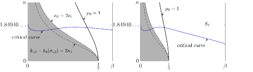
Figure 13. Left panel: Waves admitting $(k_{2},k_{4},2)\in\mathcal{R}(\sigma)$ for some $\sigma>0$ sit below the curve satisfying $k_{c,2}-k_{4}(\sigma_{c,2})=2\kappa_{1}$. Waves admitting $(k_{6},k_{4},2)\in\mathcal{R}(\sigma)$ for some $\sigma>0$ sit between the curve on which $k_{c,2}-k_{4}(\sigma_{c,2})=2\kappa_{1}$ and the curve on which $\kappa_{2}=2\kappa_{1}$, i.e., the domain of Wilton ripples of order. Waves admitting $(k_{4},k_{5},2)\in\mathcal{R}(\sigma)$ for some $\sigma>0$ sit above the curve on which $\kappa_{2}=2\kappa_{1}$, i.e., the domain of Wilton ripples of order. We find ${\rm ind}_{2}>0$ for waves admitting $(k_{2},k_{4},2)$- or $(k_{6},k_{4},2)$-resonance and ${\rm ind}_{2}<0$ for waves admitting $(k_{4},k_{5},2)$-resonance, except for waves on a critical curve (blue in color) where we find ${\rm ind}_{2}=0$. The critical curve intersect $\kappa$ axis at $\kappa=1.849404083750\ldots$, agree with the result of zero surface tension case [17]. Right panel: Plot of the critical curve for large surface tension.

5.1.5. Resonant critical frequencies with $N=1$

We now turn to the study of cases (16)-(19) in which waves admit two pairs of resonant eigenvalues at the critical frequency $-i\sigma_{c,1}$ or $i\sigma_{c,2}$. Because of the appearance of double eigenvalue $ik_{c,1}$ (resp. $-ik_{c,2}$) of $\mathbf{L}(-i\sigma_{c,1})^{\dagger}$ (resp. $\mathbf{L}(i\sigma_{c,2})^{\dagger}$), the eigenfunction defined in (3.46) (resp. (3.47)) becomes singular for $\sigma=-\sigma_{c,1}$ (resp. $\sigma=\sigma_{c,2}$) and $j=1,3$ (resp. $j=2,6$). Consequently, generalized eigenfunctions of $\mathbf{L}(-i\sigma_{c,1})^{\dagger}$ (resp. $\mathbf{L}(i\sigma_{c,2})^{\dagger}$) (see (3.49)) shall be used in the definition of the projection map $\boldsymbol{\Pi}(\sigma)$. Another main difference due to the appearance of double eigenvalue is the matrix $\mathbf{a}^{(0,0)}(x;-i\sigma_{c,1})$ (resp. $\mathbf{a}^{(0,0)}(x;i\sigma_{c,2})$) now has non-vanishing off-diagonal entry just like the case when $\sigma=0$ (3.55). Below we focus on cases (16)-(18) with $N=1$.

Lemma 5.16.

For waves discussed in cases (16)-(18) satisfying $(-1)^{r}k_{c,r}-k_{j}((-1)^{r}\sigma_{c,r})=N\kappa$, for $N=1$ or $-1$ and $r=1$ or $2$, for convenience, we switch the position of resonant modes $\boldsymbol{\phi}_{r}((-1)^{r}\sigma_{c,r})$, $\boldsymbol{\phi}_{3r}((-1)^{r}\sigma_{c,r})$, and $\boldsymbol{\phi}_{j}((-1)^{r}\sigma_{c,r})$ with the first three modes in the basis $\mathcal{B}((-1)^{r}\sigma_{c,r})$. At the resonant critical frequency $(-1)^{r}i\sigma_{c,r}$, the left top $3$ by $3$ block matrix of $\mathbf{a}^{(0,0)}(T)$ reads

$$e^{i(-1)^{r}k_{c,r}T}\begin{pmatrix}1&T&0\\ 0&1&0\\ 0&0&1\end{pmatrix},$$

the left top $3$ by $3$ block matrix of $\mathbf{a}^{(1,0)}(T)$ reads $\begin{pmatrix}a^{(1,0)}_{11}&a^{(1,0)}_{12}&0\\ a^{(1,0)}_{21}&a^{(1,0)}_{22}&0\\ 0&a^{(1,0)}_{32}&a^{(1,0)}_{33}\end{pmatrix}$, and the left top $3$ by $3$ block matrix of $\mathbf{a}^{(0,1)}(T)$ reads $\begin{pmatrix}0&a^{(0,1)}_{12}&a^{(0,1)}_{13}\\ 0&a^{(0,1)}_{22}&a^{(0,1)}_{23}\\ a^{(0,1)}_{31}&a^{(0,1)}_{32}&0\end{pmatrix}$. Moreover, there hold

$$a_{21}^{(1,0)},a_{22}^{(0,1)},a_{31}^{(0,1)}\in ie^{i(-1)^{r}k_{c,r}T}\mathbb{R},\quad a_{33}^{(1,0)},a_{23}^{(0,1)}\in e^{i(-1)^{r}k_{c,r}T}\mathbb{R}.$$ (5.26)

Proof.

For simplicity, denote $k_{c}:=(-1)^{r}k_{c,r}$ and $\sigma_{c}:=(-1)^{r}\sigma_{c,r}$. The proof is based on similar computations made in [17, Lemma 6.3]. In particular, the first three rows of the second column of $\mathbf{a}^{(0,0)}(x)$ reads $\begin{pmatrix}xe^{ik_{c}x}\\ e^{ik_{c}x}\\ 0\end{pmatrix}$ for $xe^{ik_{c}x}\boldsymbol{\phi}_{r}+e^{ik_{c}x}\boldsymbol{\phi}_{3r}$ is the solution to (3.59) (3.60) (3.51) (3.52) when $m=n=0$, $\sigma=\sigma_{c}$, and $k=2$. The second columns of $\mathbf{a}^{(0,1)}(x)$ and $\mathbf{a}^{(1,0)}(x)$ then do not necessarily vanish because of the term $xe^{ik_{c}x}\boldsymbol{\phi}_{r}$. ∎

If $Y(\sigma_{c})$ is four dimensional, let $\mathcal{B}(\sigma_{c})=\{\boldsymbol{\phi}_{r},\boldsymbol{\phi}_{3r},\boldsymbol{\phi}_{j},\boldsymbol{\phi}_{s}\}$. The periodic Evans function then expands as

$$\Delta(i\sigma_{c}+\delta,k_{c}+p\kappa+\gamma;\varepsilon)$$ (5.27)

$$= d^{(2,0,0)}\delta^{2}+d^{(1,1,0)}\gamma\delta+d^{(0,0,2)}\varepsilon^{2}+\mathchoice{{\scriptstyle\mathcal{O}}}{{\scriptstyle\mathcal{O}}}{{\scriptscriptstyle\mathcal{O}}}{\scalebox{0.7}{$\scriptscriptstyle\mathcal{O}$}}(|\delta|+|\gamma|+|\varepsilon|)^{2},$$

where

$$d^{(2,0,0)} =-Ta_{21}^{(1,0)}a_{33}^{(1,0)}(e^{iT(k_{c}+k_{s})}-e^{2iTk_{c}}),$$ (5.28)

$$d^{(1,1,0)} =iT^{2}a_{21}^{(1,0)}e^{iTk_{c}}(e^{iT(k_{c}+k_{s})}-e^{2iTk_{c}}),$$

$$d^{(0,0,2)} =Ta_{23}^{(0,1)}a_{31}^{(0,1)}(e^{iT(k_{c}+k_{s})}-e^{2iTk_{c}}).$$

For the Weierstrass’s factorization $\Delta(i\sigma_{c}+\delta,k_{c}+p\kappa+\gamma;\varepsilon)=W(\delta,\gamma,\varepsilon)h(\delta,\gamma,\varepsilon)$ (4.3), computation reveals

$$W(\delta,\gamma,\varepsilon)= \delta^{2}+\left(d^{(1,1,0)}\big{(}d^{(2,0,0)}\big{)}^{-1}\gamma+\mathchoice{{\scriptstyle\mathcal{O}}}{{\scriptstyle\mathcal{O}}}{{\scriptscriptstyle\mathcal{O}}}{\scalebox{0.7}{$\scriptscriptstyle\mathcal{O}$}}(|\gamma|+|\varepsilon|)\right)\delta$$ (5.29)

$$+d^{(0,0,2)}\big{(}d^{(2,0,0)}\big{)}^{-1}\varepsilon^{2}+\mathchoice{{\scriptstyle\mathcal{O}}}{{\scriptstyle\mathcal{O}}}{{\scriptscriptstyle\mathcal{O}}}{\scalebox{0.7}{$\scriptscriptstyle\mathcal{O}$}}\left(|\gamma|+|\varepsilon|\right)^{2}.$$

Theorem 5.17 (Resonant critical frequencies $(-1)^{r}i\sigma_{c,r}$ with $N=1$).

Consider a $(\beta,\kappa)$- non-resonant capillary-gravity wave of sufficiently small amplitude discussed in cases (16)-(18) with $N=1$ and its spectra near the resonant critical frequency $(-1)^{r}i\sigma_{c,r}$. If

$${\rm ind}_{3}(\beta(\kappa),\kappa):=\frac{a^{(0,1)}_{23}a^{(0,1)}_{31}}{a_{21}^{(1,0)}a_{33}^{(1,0)}}>0,$$ (5.30)

the wave admits unstable spectra in shape of bubble of size $\mathcal{O}(\varepsilon)$ near the resonant critical frequency $(-1)^{r}i\sigma_{c,r}$ as described in Corollary 5.18. If

$${\rm ind}_{3}(\beta(\kappa),\kappa)<0,$$ (5.31)

the wave admits no unstable spectrum near the resonant critical frequency $(-1)^{r}i\sigma_{c,r}$. To put it another way, the spectra stay on the imaginary axis near the resonant frequency $(-1)^{r}i\sigma_{c,r}$ for all sufficiently small amplitude. If

$${\rm ind}_{3}(\beta(\kappa),\kappa)=0,$$ (5.32)

stability of the spectra near the resonant frequency is determined by higher order terms of the $\mathbf{a}^{(m,n)}(T;\sigma)$ (3.50).

Proof.

The proof is similar to Theorems 5.5 and  5.9. ∎

Corollary 5.18 (Unstable spectra in shape of a circle at $\mathcal{O}(\varepsilon)$-order).

Provided that (5.30) holds, there exist, near the resonant critical frequency $(-1)^{r}i\sigma_{c,r}$, unstable spectra in shape of a bubble of size $\mathcal{O}(\varepsilon)$, which is, at the leading $\mathcal{O}(\varepsilon)$-order, a circle with equation

$$(\Re\lambda)^{2}+(\Im\lambda-(-1)^{r}i\sigma_{c,r})^{2}={\rm ind}_{3}\varepsilon^{2},$$ (5.33)

whose center is at the resonant critical frequency $(-1)^{r}i\sigma_{c,r}$.

Proof.

Dropping the $\mathchoice{{\scriptstyle\mathcal{O}}}{{\scriptstyle\mathcal{O}}}{{\scriptscriptstyle\mathcal{O}}}{\scalebox{0.7}{$\scriptscriptstyle\mathcal{O}$}}$ terms in (5.29), we solve for $\delta=\delta_{r}+i\delta_{i}$, $\delta_{r},\delta_{i}\in\mathbb{R}$, at the leading order, the equation

$$(\delta_{r}+i\delta_{i})^{2}+\frac{d^{(1,1,0)}\gamma}{d^{(2,0,0)}}(\delta_{r}+i\delta_{i})+\frac{d^{(0,0,2)}}{d^{(2,0,0)}}\varepsilon^{2}=0,$$ (5.34)

where, recalling Corollary 5.2 and (5.29), we find

$$\frac{d^{(1,1,0)}}{d^{(2,0,0)}}\in i\mathbb{R}\quad\text{and}\quad\frac{d^{(0,0,2)}}{d^{(2,0,0)}}\in\mathbb{R}.$$

Taking the imaginary part of (5.34) yields

$$\gamma=-\frac{2id^{(2,0,0)}}{d^{(1,1,0)}}\delta_{i}.$$ (5.35)

Substituting the $\gamma$ in (5.34) by the RHS of (5.35) yields (5.33). ∎

5.1.6. Resonant critical frequencies with $N=2$

We now turn to cases (16)-(19) with $N=2$. Particularly, we treat the waves in the region $-\sigma_{c,1}<\sigma_{c,2}$ and on the curve $k_{c,2}-k_{4}(\sigma_{c,2})=2\kappa$, i.e., case (19) in which $(k_{2}(\sigma_{c,2}),k_{4}(\sigma_{c,2}),2),(k_{6}(\sigma_{c,2}),k_{4}(\sigma_{c,2}),2)\in\mathcal{R}(\sigma_{c,2})$ and $Y(\sigma_{c,2})$ is four dimensional. The other cases can be treated similarly.

Lemma 5.19.

Consider a $(\beta,\kappa)$ in the region $-\sigma_{c,1}<\sigma_{c,2}$ and on the curve $k_{c,2}-k_{4}(\sigma_{c,2})=2\kappa$. See FIGURE 6 and FIGURE 9. For convenience, we reorder the basis $\mathcal{B}(\sigma_{c,2})$ as

$$\{\boldsymbol{\phi}_{2}(\sigma_{c,2}),\boldsymbol{\phi}_{6}(\sigma_{c,2}),\boldsymbol{\phi}_{4}(\sigma_{c,2}),\boldsymbol{\phi}_{5}(\sigma_{c,2})\}.$$

At the resonant critical frequency $i\sigma_{c,2}$, the left top $3$ by $3$ block matrix of $\mathbf{a}^{(0,0)}(T)$ reads

$$e^{ik_{c,2}T}\begin{pmatrix}1&T&0\\ 0&1&0\\ 0&0&1\end{pmatrix},$$

the left top $3$ by $3$ block matrix of $\mathbf{a}^{(1,0)}(T)$ reads $\begin{pmatrix}a^{(1,0)}_{11}&a^{(1,0)}_{12}&0\\ a^{(1,0)}_{21}&a^{(1,0)}_{22}&0\\ 0&a^{(1,0)}_{32}&a^{(1,0)}_{33}\end{pmatrix}$, and the left top $3$ by $3$ block matrix of $\mathbf{a}^{(0,1)}(T)$ reads $\begin{pmatrix}0&a^{(0,1)}_{12}&0\\ 0&a^{(0,1)}_{22}&0\\ 0&a^{(0,1)}_{32}&0\end{pmatrix}$.

Proof.

The proof is similar to that of Lemma 5.16. In particular, we note the first three rows of the first and third columns of $\mathbf{a}^{(0,1)}(x)$ necessarily vanish because of the higher $2$-resonance than that in Lemma 5.16. ∎

At the resonant critical frequency $i\sigma_{c,2}$, the periodic Evans function then expands as

$$\Delta(i\sigma_{c,2}+\delta,k_{c,2}+p\kappa+\gamma;\varepsilon)$$ (5.36)

$$= d^{(2,0,0)}\delta^{2}+d^{(1,1,0)}\gamma\delta+d^{(1,0,2)}\varepsilon^{2}\delta+d^{(0,1,2)}\gamma\varepsilon^{2}+d^{(0,0,4)}\varepsilon^{4}$$

$$+\mathchoice{{\scriptstyle\mathcal{O}}}{{\scriptstyle\mathcal{O}}}{{\scriptscriptstyle\mathcal{O}}}{\scalebox{0.7}{$\scriptscriptstyle\mathcal{O}$}}(|\delta|+|\gamma|+|\varepsilon^{2}|)^{2},$$

where

$$d^{(2,0,0)} =-Ta_{21}^{(1,0)}a_{33}^{(1,0)}(e^{iT(k_{c,2}+k_{5})}-e^{2iTk_{c,2}}),$$ (5.37)

$$d^{(1,1,0)} =iT^{2}a_{21}^{(1,0)}e^{iTk_{c,2}}(e^{iT(k_{c,2}+k_{5})}-e^{2iTk_{c,2}}),$$

$$d^{(1,0,2)} =Te^{iTk_{c,2}}(a_{21}^{(1,0)}a_{34}^{(0,1)}a_{43}^{(0,1)}+a_{24}^{(0,1)}a_{33}^{(1,0)}a_{41}^{(0,1)}$$

$$\quad-a_{21}^{(0,2)}a_{33}^{(1,0)}e^{iTk_{5}}-a_{21}^{(1,0)}a_{33}^{(0,2)}e^{iTk_{5}}$$

$$\quad+a_{21}^{(0,2)}a_{33}^{(1,0)}e^{iTk_{c,2}}+a_{21}^{(1,0)}a_{33}^{(0,2)}e^{iTk_{c,2}}),$$

$$d^{(0,1,2)} =-iT^{2}e^{2iTk_{c,2}}(a_{21}^{(0,2)}e^{iTk_{c,2}}-a_{21}^{(0,2)}e^{iTk_{5}}+a_{24}^{(0,1)}a_{41}^{(0,1)}),$$

$$d^{(0,0,4)} =Te^{iTk_{c,2}}(a_{21}^{(0,2)}a_{34}^{(0,1)}a_{43}^{(0,1)}-a_{23}^{(0,2)}a_{34}^{(0,1)}a_{41}^{(0,1)}$$

$$\quad-a_{24}^{(0,1)}a_{31}^{(0,2)}a_{43}^{(0,1)}+a_{24}^{(0,1)}a_{33}^{(0,2)}a_{41}^{(0,1)}$$

$$\quad-a_{21}^{(0,2)}a_{33}^{(0,2)}e^{iTk_{5}}+a_{23}^{(0,2)}a_{31}^{(0,2)}e^{iTk_{5}}$$

$$\quad+a_{21}^{(0,2)}a_{33}^{(0,2)}e^{iTk_{c,2}}-a_{23}^{(0,2)}a_{31}^{(0,2)}e^{iTk_{c,2}}).$$

Theorem 5.20 (Resonant critical frequencies $(-1)^{r}i\sigma_{c,r}$ with $N=2$).

Consider a $(\beta,\kappa)$- non-resonant capillary-gravity wave of sufficiently small amplitude in the region $-\sigma_{c,1}<\sigma_{c,2}$ and on the curve $k_{c,2}-k_{4}(\sigma_{c,2})=2\kappa$. See FIGURE 6 and FIGURE 9. Consider spectra of the wave near the resonant critical frequency $i\sigma_{c,2}$. If

$${\rm ind}_{4}(\beta(\kappa),\kappa)$$ (5.38)

$$:= -\frac{d^{(2,0,0)}(d^{(0,1,2)})^{2}-d^{(1,0,2)}d^{(0,1,2)}d^{(1,1,0)}+d^{(0,0,4)}(d^{(1,1,0)})^{2}}{(d^{(1,1,0)})^{2}d^{(2,0,0)}}>0,$$

the wave admits unstable spectra in shape of bubble of size $\mathcal{O}(\varepsilon^{2})$ near the resonant critical frequency $i\sigma_{c,2}$ as described in Corollary 5.21. If

$${\rm ind}_{4}(\beta(\kappa),\kappa)<0,$$ (5.39)

the wave admits no unstable spectrum near the resonant critical frequency $i\sigma_{c,2}$. To put it another way, the spectra stay on the imaginary axis near the resonant frequency $i\sigma_{c,2}$ for all sufficiently small amplitude. If

$${\rm ind}_{4}(\beta(\kappa),\kappa)=0,$$ (5.40)

stability of the spectra near the resonant frequency is determined by higher order terms of the $\mathbf{a}^{(m,n)}(T;\sigma)$ (3.50).

Proof.

The proof is similar to Theorems 5.5 and  5.9. ∎

Corollary 5.21 (Unstable spectra in shape of a circle at $\mathcal{O}(\varepsilon^{2})$-order).

Provided that (LABEL:def:ind_4) holds, there exist, near the resonant critical frequency $i\sigma_{c,2}$, unstable spectra in shape of a bubble of size $\mathcal{O}(\varepsilon^{2})$, which is, at the leading $\mathcal{O}(\varepsilon^{2})$-order, a circle with equation

$$(\Re\lambda)^{2}+(\Im\lambda-i\sigma_{c,2}-i\frac{d^{(0,1,2)}}{d^{(1,1,0)}}\varepsilon^{2})^{2}={\rm ind}_{4}\varepsilon^{4},$$ (5.41)

whose center drifts from the resonant critical frequency $i\sigma_{c,2}$ by a distance of $-i\frac{d^{(0,1,2)}}{d^{(1,1,0)}}\varepsilon^{2}$.

Proof.

From the proofs of Corollaries 5.6, 5.11, and 5.18 and equations (LABEL:expanddeltaresonance1) versus (5.3), (LABEL:expanddeltaresonance1_cri) versus (5.29), we can, without writing down the Weierstrass polynomial, drop the $\mathchoice{{\scriptstyle\mathcal{O}}}{{\scriptstyle\mathcal{O}}}{{\scriptscriptstyle\mathcal{O}}}{\scalebox{0.7}{$\scriptscriptstyle\mathcal{O}$}}$- terms of (LABEL:expanddeltaresonance2_cri) to solve at the leading order for $\delta=\delta_{r}+i\delta_{i}$, $\delta_{r},\delta_{i}\in\mathbb{R}$. The imaginary part of the equation gives

$$\gamma=-\frac{d^{(1,0,2)}}{d^{(1,1,0)}}\varepsilon^{2}-\frac{2id^{(2,0,0)}}{d^{(1,1,0)}}\delta_{i}.$$

Substituting the $\gamma$ in the leading part of (LABEL:expanddeltaresonance2_cri) by the RHS above yields (5.41). ∎

Remark 7.

Comparing Corollary 5.18 with Corollary 5.21, we note that the circle of unstable spectra does not drift from the resonant critical frequency $(-1)^{r}i\sigma_{c,r}$ with two pairs of $1$-resonant eigenvalues, while the circle of unstable spectra drifts from the resonant critical frequency with two pairs of $2$-resonant eigenvalues by a $\mathcal{O}(\varepsilon^{2})$-distance.

Remark 8.

Comparing Corollaries 5.6 and  5.11 with Corollaries 5.18 and  5.21, we note that, near resonant non-critical frequencies, the shape of unstable spectra is, at the leading order, an ellipse, while, near resonant critical frequencies, the shape of unstable spectra is, at the leading order, a circle.

5.1.7. Numerical results

By Theorem 5.17, the index function ${\rm ind}_{3}$ (5.30) can be used to examine the stability at the critical frequency $-i\sigma_{c,1}$ or $i\sigma_{c,2}$, i.e., cases (16)-(18) with $N=1$. By Theorem 5.20, the index function ${\rm ind}_{4}$ (LABEL:def:ind_4) can be used to examine the stability for waves in case (19) and in the region $-\sigma_{c,1}<\sigma_{c,2}$. For waves discussed in other situations of cases (16)-(19) with $N=2$, we also obtain index functions denoted still as ${\rm ind}_{4}(\beta(\kappa),\kappa)$.

For $(\beta,\kappa)$ in the super-critical region with $\kappa<8$, we document numerical findings for unstable waves at critical frequencies $-i\sigma_{c,1}$ and $i\sigma_{c,2}$ below.

• For waves on the curve satisfying $-k_{c,1}-k_{5}(-\sigma_{c,1})=\kappa$ (see FIGURE 6 right panel), we find numerically ${\rm ind}_{3}(\beta(\kappa),\kappa)<0$. Hence, for all of these waves, spectra in the vicinity of the resonant frequency are purely imaginary;
  For waves on the curve satisfying $-k_{c,1}-k_{5}(-\sigma_{c,1})=2\kappa$ (see FIGURE 6 right panel), we find numerically ${\rm ind}_{4}(\beta(\kappa),\kappa)<0$. Hence, for all of these waves, spectra in the vicinity of the resonant frequency are purely imaginary;

• For waves on the curve satisfying $k_{6}(-\sigma_{c,1})+k_{c,1}=\kappa$ (see FIGURE 7 left panel), we find numerically ${\rm ind}_{3}(\beta(\kappa),\kappa)>0$. Hence, for all of these waves, there are unstable spectra in the vicinity of the resonant frequency;
  For waves on the curve satisfying $k_{c,2}-k_{1}(\sigma_{c,2})=\kappa$ (see FIGURE 7 left panel), we find numerically ${\rm ind}_{3}(\beta(\kappa),\kappa)>0$. Hence, for all of these waves, there are unstable spectra in the vicinity of the resonant frequency;
  For waves on the curve satisfying $k_{6}(-\sigma_{c,1})+k_{c,1}=2\kappa$ (see FIGURE 7 right panel), we find numerically ${\rm ind}_{4}(\beta(\kappa),\kappa)>0$. Hence, for all of these waves, there are unstable spectra in the vicinity of the resonant frequency;
  For waves on the curve satisfying $k_{c,2}-k_{1}(\sigma_{c,2})=2\kappa$ (see FIGURE 7 right panel), we find numerically ${\rm ind}_{4}(\beta(\kappa),\kappa)>0$. Hence, for all of these waves, there are unstable spectra in the vicinity of the resonant frequency;

• For waves on the curve satisfying $k_{2}(-\sigma_{c,1})+k_{c,1}=\kappa$ (see FIGURE 8 right panel), we find numerically ${\rm ind}_{3}(\beta(\kappa),\kappa)>0$. Hence, for all of these waves, there are unstable spectra in the vicinity of the resonant frequency;
  For waves on the curve satisfying $k_{c,2}-k_{3}(\sigma_{c,2})=\kappa$ (see FIGURE 8 right panel), we find numerically ${\rm ind}_{3}(\beta(\kappa),\kappa)>0$. Hence, for all of these waves, there are unstable spectra in the vicinity of the resonant frequency;
  For waves on the curve satisfying $k_{2}(-\sigma_{c,1})+k_{c,1}=2\kappa$ (see FIGURE 8 left panel), we find numerically ${\rm ind}_{4}(\beta(\kappa),\kappa)>0$. Hence, for all of these waves, there are unstable spectra in the vicinity of the resonant frequency;
  For waves on the curve satisfying $k_{c,2}-k_{3}(\sigma_{c,2})=2\kappa$ (see FIGURE 8 left panel), we find numerically ${\rm ind}_{4}(\beta(\kappa),\kappa)>0$. Hence, for all of these waves, there are unstable spectra in the vicinity of the resonant frequency;

• For waves on the curve satisfying $k_{c,2}-k_{4}(\sigma_{c,2})=2\kappa$ (see FIGURE 9 left panel), we find numerically ${\rm ind}_{4}(\beta(\kappa),\kappa)>0$. Hence, for all of these waves, there are unstable spectra in the vicinity of the resonant frequency.

Remark 9.

By (17) (resp. (18)), the instability of waves studied in (6) (resp. (7)) continues to the boundaries. See FIGURE 7 (resp. FIGURE 8).

By (19), the instability of waves studied in (9) and (11) continues to the boundary $k_{c,2}-k_{4}(\sigma_{c,2})=2\kappa_{1}$. See FIGURE 13.

Taking unions of non-resonant capillary-gravity waves from (1)-(19) that admit unstable spectra near the resonant (critical) frequencies $i\sigma$ with $N=1$ and $N=2$, respectively, we make FIGURE 1 top right panel.

5.2. The spectrum near the origin

In this section, we turn the attention to the origin $\lambda=0$. Since $\lambda=0$ is a resonant frequency, Theorem 4.5 implies that spectra are possibly off the imaginary axis near $0$, giving instability. The spectral stability we investigate here corresponds to the formal modulational stability and we will show later they do agree.

Lemma 5.22.

For $n\geqslant 1$, the fourth column of the matrix $\mathbf{a}^{(0,n)}(x;0)$ in the expansion of $\mathbf{X}(x;0,0,\varepsilon)$ (3.50) corresponding to the mode $\boldsymbol{\phi}_{4}(0)$ in (3.21) and (3.24) vanishes when $x=T$.

Proof.

In the original coordinate, when $\lambda=0$, we find $\phi$=constant, $u=\eta=z=0$ solves (3.2). Setting the constant to be $(1+\eta(0;\varepsilon))(1-u(0,1;\varepsilon))(1+\eta_{x}(0;\varepsilon)^{2})^{3/2}$ and working in the new unknown (3.3), we find

$$\mathbf{u}(x)=\begin{pmatrix}\frac{(1+\eta(0;\varepsilon))(1-u(0,1;\varepsilon))(1+\eta_{x}(0;\varepsilon)^{2})^{3/2}}{(1+\eta(x;\varepsilon))(1-u(x,1;\varepsilon))(1+\eta_{x}(x;\varepsilon)^{2})^{3/2}}\\ 0\\ 0\\ 0\end{pmatrix}$$

shall solve (3.10) for $\lambda=0$. Because $\mathbf{u}(x)$ is a multiple of the mode $\boldsymbol{\phi}_{4}(0)$ in (3.21) and (3.24), in (3.26), we have $\mathbf{v}(x)=\boldsymbol{\Pi}(\sigma)\mathbf{u}(x)=\mathbf{u}(x)$. Also, by the uniqueness of solution of the ordinary differential equation (3.26), or, equivalently, (3.38), because $\mathbf{v}(0)=\boldsymbol{\phi}_{4}(0)=\mathbf{v}_{4}(0;0,0,\varepsilon)$ in (3.51), $\mathbf{v}(x)=\mathbf{v}_{4}(x;0,0,\varepsilon)$ for all $x$. Hence $\mathbf{v}_{4}(T;0,0,\varepsilon)=\mathbf{u}(T)=\mathbf{u}(0)=\boldsymbol{\phi}_{4}(0)$ by periodicity of the profile. Noticing that

$$\sum_{n=0}^{\infty}a^{(0,n)}_{j4}(T;0)\varepsilon^{n}=\langle\mathbf{v}_{4}(T;0,0,\varepsilon),\boldsymbol{\psi}_{j}(0)\rangle,$$

$a^{(0,n)}_{j4}(T;0)$ then vanishes for $n\geqslant 1$ because the right hand side of the equation above is independent of $\varepsilon$. ∎

Corollary 5.23.

For $\varepsilon\in\mathbb{R}$ and $|\varepsilon|\ll 1$, $\Delta(0,p\kappa;\varepsilon)=0$, $p\in\mathbb{Z}$.

Proof.

Notice that $\Delta(0,p\kappa;\varepsilon)=\det(\mathbf{I}-\mathbf{X}(T;0,0,\varepsilon))$, and Lemma 5.22 and (3.52) assert that the fourth column of $\mathbf{I}-\mathbf{X}(T;0,0,\varepsilon)$ vanishes. ∎

For waves in the sub-critical region, $\mathbf{a}^{(m,n)}(T;0)$ are 4 by 4 matrices. Carrying out the computations outlined in Section 3.6 gives the following lemma.

Lemma 5.24.

Computations show

$$\mathbf{a}^{(1,0)}(T;0)=\begin{pmatrix}a^{(1,0)}_{11}&0&a^{(1,0)}_{13}&0\\ 0&a^{(1,0)}_{11}&-a^{(1,0)}_{13}&0\\ 0&0&a^{(1,0)}_{33}&0\\ a^{(1,0)}_{41}&a^{(1,0)}_{41}&Ta^{(1,0)}_{33}&a^{(1,0)}_{33}\end{pmatrix},$$ (5.42)

$$\mathbf{a}^{(0,1)}(T;0)=\begin{pmatrix}0&0&a^{(0,1)}_{13}&0\\ 0&0&a^{(0,1)}_{13}&0\\ 0&0&0&0\\ a^{(0,1)}_{41}&-a^{(0,1)}_{41}&*&0\end{pmatrix},$$ (5.43)

$$\mathbf{a}^{(2,0)}(T;0)=\begin{pmatrix}a_{11}^{(2,0)}&-a_{21}^{(2,0)}&*&a_{14}^{(2,0)}\\ a_{21}^{(2,0)}&(a_{11}^{(2,0)})^{*}&*&-a_{14}^{(2,0)}\\ a_{31}^{(2,0)}&a_{31}^{(2,0)}&a_{33}^{(2,0)}&a_{34}^{(2,0)}\\ *&*&*&a_{33}^{(2,0)}\end{pmatrix},$$ (5.44)

$$\mathbf{a}^{(1,1)}(T;0)=\begin{pmatrix}a_{11}^{(1,1)}&a_{21}^{(1,1)}&*&a_{14}^{(1,1)}\\ a_{21}^{(1,1)}&a_{11}^{(1,1)}&*&a_{14}^{(1,1)}\\ a_{31}^{(1,1)}&-a_{31}^{(1,1)}&*&0\\ *&*&*&*\end{pmatrix},$$ (5.45)

$$\mathbf{a}^{(0,2)}(T;0)=\begin{pmatrix}a_{11}^{(0,2)}&-a_{11}^{(0,2)}&*&0\\ a_{11}^{(0,2)}&-a_{11}^{(0,2)}&*&0\\ 0&0&*&0\\ *&*&*&0\end{pmatrix},$$ (5.46)

where $a^{(1,0)}_{11}$, $a^{(1,0)}_{13}$ $a^{(1,0)}_{33}$ $a^{(1,0)}_{41}$, $a^{(0,1)}_{13}$, $a^{(0,1)}_{41}$, $a^{(2,0)}_{11}$, $a^{(2,0)}_{34}$, $a^{(1,1)}_{31}$, $a^{(1,1)}_{14}$, and $a^{(0,2)}_{11}$ are given in Appendix D. Our computations also show there hold

$$a^{(2,0)}_{21}=-a^{(1,0)}_{13}a^{(1,0)}_{41}/T,\quad a_{14}^{(2,0)}=-a_{13}^{(1,0)}\big{(}a_{11}^{(1,0)}-a_{33}^{(1,0)}\big{)}/T,$$ (5.47)

$$a_{31}^{(2,0)}=-a_{41}^{(1,0)}\big{(}a_{11}^{(1,0)}-a_{33}^{(1,0)}\big{)}/T,$$

$$a_{11}^{(1,1)}=\big{(}a_{13}^{(0,1)}a_{41}^{(1,0)}+a_{13}^{(1,0)}a_{41}^{(0,1)}\big{)}/T,$$

$$a_{21}^{(1,1)}=\big{(}a_{13}^{(0,1)}a_{41}^{(1,0)}-a_{13}^{(1,0)}a_{41}^{(0,1)}\big{)}/T,$$

and we use these relations together with the relations shown in (5.42), (5.43), (5.44), (5.45), and (5.46) to make simplification in the later expansion of the periodic Evans function (5.48). Our analysis does not involve other entries marked with $*$ of $\mathbf{a}^{(0,1)}(T;0)$, $\mathbf{a}^{(2,0)}(T;0)$, $\mathbf{a}^{(1,1)}(T;0)$, and $\mathbf{a}^{(0,2)}(T;0)$, whence we do not include the formulas here. We make clear that $a_{22}^{(2,0)}$ in (5.44) is the complex conjugate of $a_{11}^{(2,0)}$ and we also do not include formulas for $a_{33}^{(2,0)}$ and $a_{44}^{(2,0)}$ but merely use $a_{33}^{(2,0)}=a_{44}^{(2,0)}$ as noted in (5.44).

Proof.

The Lemma follows from direct computations outlined in Section 3.6. ∎

At $(0,p\kappa;0)$, putting together (3.55), (5.42), (5.43), (5.44), (5.45), (5.46), (LABEL:extra_relation) yields

$$\Delta(\delta,p\kappa+\gamma;\varepsilon)= \sum_{l=0}^{4}d^{(l,4-l,0)}\delta^{l}\gamma^{4-l}+\sum_{l=0}^{3}d^{(l,3-l,2)}\delta^{l}\gamma^{3-l}\varepsilon^{2}$$ (5.48)

$$+\mathchoice{{\scriptstyle\mathcal{O}}}{{\scriptstyle\mathcal{O}}}{{\scriptscriptstyle\mathcal{O}}}{\scalebox{0.7}{$\scriptscriptstyle\mathcal{O}$}}\big{(}(|\delta|+|\gamma|)^{3}(|\delta|+|\gamma|+|\varepsilon|^{2})\big{)},$$

as $\delta,\gamma,\varepsilon\to 0$, where, analogous to (5.2), (5.28), and (5.37), $d^{(\ell,m,n)}$, $\ell,m,n=0,1,2,\dots$ can be determined in terms of $\mathbf{a}^{(m,n)}(T;0)$, $m,n=0,1,2,\dots$. We omit the formulas. Nonetheless, we note that, by (D.1) and (D.3)

$$d^{(4,0,0)}= \left(a_{11}^{(1,0)}\right)^{2}\left(\left(a_{33}^{(1,0)}\right)^{2}-Ta_{34}^{(2,0)}\right)$$

$$= 64\pi^{4}{\,{\rm sh}(2\kappa)}^{2}\,{\rm sh}(\kappa)\left(\beta\kappa^{2}+1\right)^{3}\cdot\Big{(}\kappa^{4}\left(\,{\rm sh}(\kappa)-\kappa\,{\rm ch}(\kappa)+\beta\kappa^{2}\,{\rm sh}(\kappa)\right)$$

$$\cdot\left(2\kappa-\,{\rm sh}(2\kappa)+2\beta\kappa^{3}+\beta\kappa^{2}\,{\rm sh}(2\kappa)\right)^{2}\Big{)}^{-1}\neq 0.$$

The Weierstrass polynomial (4.4) is thus quartic

$$W(\delta,\gamma,\varepsilon)=\delta^{4}+a_{3}(\gamma,\varepsilon)\delta^{3}+a_{2}(\gamma,\varepsilon)\delta^{2}+a_{1}(\gamma,\varepsilon)\delta+a_{0}(\gamma,\varepsilon),$$ (5.49)

where we infer from setting $m=4$ in (4.6) that

$$a_{3}(\gamma,\varepsilon),a_{1}(\gamma,\varepsilon)\in i\mathbb{R}\quad\text{and}\quad a_{2}(\gamma,\varepsilon),a_{0}(\gamma,\varepsilon)\in\mathbb{R}.$$ (5.50)

When $\varepsilon=0$, the four zeros of (5.49) are given by $\delta_{j}(\gamma,0)=i\sigma(k_{j}(0)+\gamma)$, where $\sigma$ (3.18) admits power series expansions about $\gamma=0$. Hence,

$$\delta_{j}(\gamma,0)=\delta^{(1,0)}_{j}\gamma+\delta^{(2,0)}_{j}\gamma^{2}+\cdots,\quad\text{for $|\gamma|\ll 1$.}$$

Also, Corollary 5.23 says that $\delta=0$ is a root of $\Delta(\cdot,p\kappa;\varepsilon)$ for all $p\in\mathbb{Z}$ for $\varepsilon\in\mathbb{R}$ and $|\varepsilon|\ll 1$. Substituting

$$\delta_{j}(k_{j}(0)+\gamma,\varepsilon)=\delta^{(1,0)}_{j}\gamma+\delta^{(2,0)}_{j}\gamma^{2}+\delta^{(1,1)}_{j}\gamma\varepsilon+\cdots.$$ (5.51)

into (5.48), after straightforward calculations, we learn that $\gamma^{4}$ is the leading order whose coefficient reads

$$-\big{(}-a_{11}^{(1,0)}\delta^{(1,0)}_{j}+iT\big{)}^{2}\big{(}(Ta_{34}^{(2,0)}-{a_{33}^{(1,0)}}^{2})(\delta^{(1,0)}_{j})^{2}+2iTa_{33}^{1,0}\delta^{(1,0)}_{j}+T^{2}\big{)},$$ (5.52)

where $a_{11}^{(1,0)}$, $a_{33}^{(1,0)}$, $a_{34}^{(2,0)}$ are in (D.1) and (D.3). The coefficient of $\gamma^{4}$ (5.52) must vanish, whence

$$\delta^{(1,0)}_{j}=iT/a_{11}^{(1,0)}\quad\text{or}\quad\delta^{(1,0)}_{j}=\frac{iTa_{33}^{(1,0)}\pm\sqrt{-T^{3}a^{(2,0)}_{34}}}{(a_{33}^{(1,0)})^{2}-Ta_{34}^{(2,0)}}.$$ (5.53)

Notice that $\delta^{(1,0)}_{j}$, $j=2,4,5,6$, are purely imaginary by (D.1) and (D.3). On the other hand, (5.53) must agree with power series expansions of (3.19) about $k_{j}(0)$, $j=2,4,5,6$. Thus

$$\delta^{(1,0)}_{j}=iT/a_{11}^{(1,0)}\quad\text{for}\quad j=5,6,$$ (5.54)

and the latter equation of (5.53) holds for $j=2,4$.

Substituting (5.51) and (5.54) into (5.48), after straightforward calculations, we verify that the $\gamma^{5}$ term vanishes, and solving at the order of $\gamma^{6}$, we arrive at

$$\delta^{(2,0)}_{j}=\pm\frac{T^{2}\left((a_{11}^{(1,0)})^{2}-2a_{11}^{(2,0)}\right)+2Ta_{13}^{(1,0)}a_{41}^{(1,0)}}{2(a_{11}^{(1,0)})^{3}},\quad j=5,6,$$ (5.55)

where $a_{11}^{(1,0)}$, $a_{13}^{(1,0)}$, $a_{41}^{(1,0)}$ and $a_{11}^{(2,0)}$ are in (D.1) and (D.3). We remark that $\delta^{(2,0)}_{j}$, $j=5,6$, are purely imaginary because $(a_{11}^{(1,0)})^{2}$ offsets the real part of $2a_{11}^{(2,0)}$. The $\pm$ signs explain the oppositeness of the convexity of the curves (3.19) at $k_{j}(0)$, $j=5,6$. See Figure 5.

To proceed, substituting (5.51) into (5.48) and evaluating at (5.54) and (5.55), after straightforward calculations, we verify that the $\gamma^{3}\varepsilon^{2}$ term vanishes, and the coefficient of $\gamma^{4}\varepsilon^{2}$ reads

$$T^{2}g_{1}(\delta_{j}^{(1,1)})^{2}-T^{3}g_{2},$$ (5.56)

where

$$g_{1}= Ta_{34}^{(2,0)}+2a_{11}^{(1,0)}a_{33}^{(1,0)}-(a_{33}^{(1,0)})^{2}-(a_{11}^{(1,0)})^{2},$$ (5.57)

$$g_{2}= -(a_{11}^{(1,0)})^{-4}\big{(}T(a^{(1,0)}_{11})^{2}-2Ta^{(2,0)}_{11}+2a^{(1,0)}_{13}a^{(1,0)}_{41}\big{)}$$

$$\times\big{(}a^{(0,2)}_{11}(a^{(1,0)}_{11})^{2}+a^{(0,2)}_{11}(a^{(1,0)}_{33})^{2}-Ta^{(0,2)}_{11}a^{(2,0)}_{34}+Ta^{(1,1)}_{14}a^{(1,1)}_{31}$$

$$-2a^{(0,2)}_{11}a^{(1,0)}_{11}a^{(1,0)}_{33}+a^{(1,0)}_{11}a^{(0,1)}_{13}a^{(1,1)}_{31}+a^{(1,0)}_{11}a^{(1,1)}_{14}a^{(0,1)}_{41}$$

$$-a^{(0,1)}_{13}a^{(1,1)}_{31}a^{(1,0)}_{33}+a^{(0,1)}_{13}a^{(2,0)}_{34}a^{(0,1)}_{41}-a^{(1,1)}_{14}a^{(1,0)}_{33}a^{(0,1)}_{41}\big{)}$$

are given in (E.1).

Theorem 5.25 (Spectral instability near $0\in\mathbb{C}$ at $\gamma\varepsilon$ order).

In the sub-critical region, a $(\beta,\kappa)$- non-resonant capillary-gravity wave of sufficiently small amplitude is spectrally unstable in the vicinity of $0\in\mathbb{C}$ provided that

$${\rm ind}_{5}(\beta,\kappa):={\rm ind}_{5,1}{\rm ind}_{5,2}{\rm ind}_{5,3}{\rm ind}_{5,4}>0,$$ (5.58)

where ${\rm ind}_{5,i}$, $i=1,2,3,4$ are given in (E.2).

Proof.

The coefficient of $\gamma^{4}\varepsilon^{2}$ (5.56) must vanish, whence

$$\delta^{(1,1)}_{j}=\pm\sqrt{Tg_{2}/g_{1}},$$ (5.59)

where $g_{1}$ and $g_{2}$ are in (5.57) (E.1), and $\delta^{(1,1)}_{j}\in\mathbb{R}$ implies spectral instability. By (E.1), the sign of $g_{2}/g_{1}$ is the same as that of ${\rm ind}_{5,2}{\rm ind}_{5,3}/\left({\rm ind}_{5,1}{\rm ind}_{5,4}\right)$ and hence that of ${\rm ind}_{5}$. Therefore, (5.59) is real if ${\rm ind}_{5}(\kappa)>0$. This completes the proof. ∎

For capillary-gravity waves in the super-critical regions where $\mathbf{a}^{(m,n)}(T;0)$ are 6 by 6 matrices, we can likewise carry out the computations outlined in Section 3.6 and similarly obtain stability index functions.

We notice, in particular, the stability index function (5.58) continues through the boundary between $S_{2}$ and $S_{3}$ region and the index for waves in the $S_{2}$ region agree with the index for waves in the $S_{3}$ region. We hence use (5.58) also to investigate the spectral stability near the origin for capillary-gravity waves in the super-critical region.

Observing that ${\rm ind}_{5,i}(\beta,\kappa)$ is a polynomial in $\beta$ of order $2$ for $i=1$, $2$ for $i=2$, $4$ for $i=3$, and $1$ for $i=4$, respectively. The curves where ${\rm ind}_{5,i}(\beta,\kappa)=0$, $i=1,2,3,4$ (E.2) are explicitly computable. These curves separate regions where ${\rm ind}_{5}(\beta,\kappa)$ is positive from those where ${\rm ind}_{5}(\beta,\kappa)$ is negative. In particular,

• Solving ${\rm ind}_{5,1}=0$ yields two real roots $\beta(\kappa)$ with opposite signs. Because $\beta>0$, we keep the positive root and denote it as $\beta_{4}(\kappa)$.

• Solving ${\rm ind}_{5,2}=0$ yields two real roots $\beta(\kappa)$ with opposite signs. We denote the positive root as $\beta_{2}(\kappa)$.

• Solving ${\rm ind}_{5,3}=0$ yields four roots $\beta(\kappa)$. The first root is positive real for $\kappa>0$ and we denote it as $\beta_{5}(\kappa)$. The second root is positive real when $0<\kappa<\kappa_{*}$ where $\kappa_{*}=1.3627\ldots$ is the critical wave number of Benjamin-Feir modulational instability and the root becomes negative when $\kappa>\kappa_{*}$. We denote this root by $\beta_{1}(\kappa)$. The third and fourth roots are negative reals when $0<\kappa<0.32\ldots$ and a pair of conjugate complex numbers with negative real part when $\kappa>0.32\ldots$. We drop these two roots.

• Solving ${\rm ind}_{5,4}=0$ yields one root $\beta(\kappa)$. The root is positive real for $\kappa>0$ and we denote the root as $\beta_{3}(\kappa)$. Indeed ${\rm ind}_{5,4}=0$ is equivalent to (LABEL:wilton_con) with $M=2$. Hence $(\kappa,\beta_{3}(\kappa))$ corresponds to the domain of Wilton ripples of order 2.

We plot $(\kappa,\beta_{i}(\kappa))$ for $i=1,2,3,4,5$ in FIGURE 14.

Remark 10.

Setting $\beta=0$, ${\rm ind}_{5,3}$ becomes

$${\rm ind}_{5,3}(\kappa,0)=-64e^{8\kappa}{\rm ind}_{1}(\kappa)$$

where the index function ${\rm ind}_{1}$ on the right hand side is the index function for Benjamin-Feir modulational instability defined in [17, eq. (5.34)] . Hence although (1.5) becomes singular when $\beta=0$, our index function is valid for the zero surface tension case.

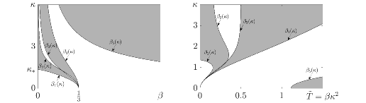
Figure 14. Modulational stability diagrams. Non-resonant capillary-gravity waves in the shaded regions are modulationally unstable. Left panel: the diagram in $\beta$ versus $\kappa$ coordinates. Notice that $\beta_{2}(\kappa)$ and $\beta_{3}(\kappa)$ intersect at $\kappa_{*}=1.28523\cdots$. Right panel: the diagram in $\tilde{T}=\beta\kappa^{2}$ versus $\kappa$ coordinates. The right panel turns out to be the same as the modulational stability diagram of Djordjevic and Redekopp’s [11, FIGURE 1].

6. Spectral instability of Wilton ripples

The general analysis framework introduced in Sections 3 and  4 applies also to the stability analysis for Wilton ripples of order $M\geqslant 2$. In particular, when we deal with system (3.26), the singularities occur in the higher $\mathcal{O}(\varepsilon^{M})$ terms of the profile (2.2) cause no changes to the leading operator $\mathbf{L}(i\sigma)$ and projection map $\boldsymbol{\Pi}(\sigma)$. The only change is we shall supply the operator $\mathbf{B}(x;\sigma,\delta,\varepsilon)$ with expansion terms of the Wilton ripples of order $2$ (LABEL:wilton2_1) (2.17) (A.1) (A.2) and terms of the Wilton ripples of order $M\geqslant 3$ (LABEL:wiltonm_1) (2.19) (LABEL:phi2_m) (LABEL:eta2_m) (A.5) (A.7).

6.1. The spectrum away from the origin

6.1.1. Wilton ripples of order $2$

By the discussion in Section 4.2, we see the domain of existence of Wilton ripples of order $2$, (LABEL:wilton_con) with $M=2$, (see FIGURE 6 right panel) can cross the domains of waves admitting $(k_{j}(\sigma),k_{j^{\prime}}(\sigma),2)\in\mathcal{R}(\sigma)$ for some $\sigma>0$. At the resonant frequency $i\sigma$, supplying the operator $\mathbf{B}(x;\sigma,\delta,\varepsilon)$ in (3.26)[i] with the profile of the Wilton ripples of order $2$ (LABEL:wilton2_1) and solving the equation yields the following lemma.

Lemma 6.1.

For Wilton ripples of order $2$ admitting $(k_{j}(\sigma),k_{j^{\prime}}(\sigma),2)\in\mathcal{R}(\sigma)$ (see cases (i)-(v) discussed above). For convenience, we switch the position of resonant modes $\boldsymbol{\phi}_{j}$ and $\boldsymbol{\phi}_{j^{\prime}}$ with first two modes in the basis $\mathcal{B}(\sigma)$ so that the resonance happens between the first two modes of $\mathcal{B}(\sigma)$. At the resonant frequency $i\sigma$, the left top $2$ by $2$ block matrix of $\mathbf{a}^{(0,0)}(T)$ reads $e^{ik_{j}T}\begin{pmatrix}1&0\\ 0&1\end{pmatrix}$, the off-diagonal entries of the left top $2$ by $2$ block matrix of $\mathbf{a}^{(1,0)}(T)$ necessarily vanish and the diagonal entries are given in (4.8) with $j$ set to $j$ and $j^{\prime}$, and entries of the left top $2$ by $2$ block matrix of $\mathbf{a}^{(0,1)}(T)$ do not necessarily vanish.

Proof.

The proof is mostly the same as [17, Lemma 6.3] except that the diagonal entries of $\mathbf{a}^{(0,1)}(T)$ do not necessarily vanish because the integral of $(\mathbf{B}^{(0,1)}(x;\sigma)\boldsymbol{\psi}_{j}(\sigma))_{4}$ (C.2) over one period is non-zero for $\mu_{1}$ (2.17) is non-zero and the off-diagonal entries of $\mathbf{a}^{(0,1)}(T)$ do not necessarily vanish because presences of $\,{\rm s}(2\kappa x)$ in $\phi_{1}$ and $\,{\rm c}(2\kappa x)$ in $\eta_{1}$ (LABEL:wilton2_1) make integrals of $e^{\pm 2i\kappa x}\,{\rm s}(2\kappa x)$ and $e^{\pm 2i\kappa x}\,{\rm c}(2\kappa x)$ over one period non-vanishing. ∎

At the resonant frequency $i\sigma$, the periodic Evans function then expands as

$$\Delta(i\sigma+\delta,k_{j}(\sigma)+p\kappa+\gamma;\varepsilon)$$ (6.1)

$$= d^{(2,0,0)}\delta^{2}+d^{(1,1,0)}\gamma\delta+d^{(1,0,1)}\varepsilon\delta+d^{(0,2,0)}\gamma^{2}+d^{(0,1,1)}\gamma\varepsilon+d^{(0,0,2)}\varepsilon^{2}$$

$$+\mathchoice{{\scriptstyle\mathcal{O}}}{{\scriptstyle\mathcal{O}}}{{\scriptscriptstyle\mathcal{O}}}{\scalebox{0.7}{$\scriptscriptstyle\mathcal{O}$}}((|\delta|+|\gamma|+|\varepsilon|)^{2}).$$

Following a similar analysis as that for Theorem 5.5, we obtain the theorem below.

Theorem 6.2 (Wilton ripples of order $2$; $(k_{j}(\sigma),k_{j^{\prime}}(\sigma),2)\in\mathcal{R}(\sigma)$).

Consider a Wilton ripples of order $2$ of sufficiently small amplitude that admits $(k_{j}(\sigma),k_{j^{\prime}}(\sigma),2)\in\mathcal{R}(\sigma)$ for some $\sigma\in\mathbb{R}$ and its spectra near the resonant frequency $i\sigma$. If

$${\rm ind}_{6}(\kappa,\sigma,k_{j}(\sigma),k_{j^{\prime}}(\sigma)):=\frac{a_{12}^{(0,1)}a_{21}^{(0,1)}}{\alpha^{2}a_{11}^{(1,0)}a_{22}^{(1,0)}}>0,$$ (6.2)

the wave admits unstable spectra in shape of a bubble of size $\mathcal{O}(\varepsilon)$ near the resonant frequency $i\sigma$ as described in Corollary 6.3. If

$${\rm ind}_{6}(\kappa,\sigma,k_{j}(\sigma),k_{j^{\prime}}(\sigma))<0,$$ (6.3)

the wave admits no unstable spectrum near the resonant frequency $i\sigma$. To put it another way, the spectra stay on the imaginary axis near the resonant frequency $i\sigma$ for all sufficiently small amplitude. If

$${\rm ind}_{6}(\kappa,\sigma,k_{j}(\sigma),k_{j^{\prime}}(\sigma)))=0,$$ (6.4)

stability of the spectra near the resonant frequency is determined by higher order terms of the $\mathbf{a}^{(m,n)}(T;\sigma)$ (3.50). The index function

$${\rm ind}_{6}(\kappa,\sigma,k_{j}(\sigma),k_{j^{\prime}}(\sigma))$$

is independent of the parameter $\alpha$ in (LABEL:wilton2_1) (2.17).

Proof.

Following a similar analysis to Theorems 5.5 and  5.9, we shall define an index function as $a^{(0,1)}_{12}a^{(0,1)}_{21}(a_{11}^{(1,0)}a_{22}^{(1,0)})^{-1}$, which can be made to be independent of $\alpha$ by dividing $\alpha^{2}$. ∎

Corollary 6.3 (Unstable spectra in shape of an ellipse at $\mathcal{O}(\varepsilon)$-order).

Provided that (6.2) holds, there exist, near the resonant frequency $i\sigma$, unstable spectra in shape of a bubble of size $\mathcal{O}(\varepsilon)$, which is, at the leading $\mathcal{O}(\varepsilon)$-order, an ellipse with equation

$$(\Re\lambda)^{2}+\left(\frac{a^{(1,0)}_{11}-a^{(1,0)}_{22}}{a^{(1,0)}_{11}+a^{(1,0)}_{22}}\right)^{2}\left(\Im\lambda-i\sigma-\frac{i(a_{11}^{(0,1)}-a_{22}^{(0,1)})}{a_{11}^{(1,0)}-a_{22}^{(1,0)}}\varepsilon\right)^{2}={\rm ind}_{6}\alpha^{2}\,\varepsilon^{2},$$ (6.5)

whose center drifts from the resonant frequency $i\sigma$ by a distance of

$$-\frac{i(a_{11}^{(0,1)}-a_{22}^{(0,1)})}{a_{11}^{(1,0)}-a_{22}^{(1,0)}}\varepsilon.$$

Proof.

The proof is similar to Corollary 5.6. ∎

In contrast to the spectral invariance under the coordinate change $\varepsilon\rightarrow-\varepsilon$ for Wilton ripples of order $M$ with $M$ odd (see Lemma 5.14), we note that the invariance unholds for Wilton ripples of order $2$ for the coordinate change flips the sign of the drifting distance in (6.5).

6.1.2. Numerical results

The domain of Wilton ripples of order $2$ can cross the domains of waves admitting $(k_{j}(\sigma),k_{j^{\prime}}(\sigma),2)\in\mathcal{R}(\sigma)$ for some $\sigma>0$ and $(j,j^{\prime})=(1,5),\;(3,5),\;(2,1),\;(2,3),\;(6,3).$ In particular,

• when $2.811980\ldots<\kappa$, the corresponding Wilton ripples of order $2$ admit

  $$(k_{1}(\sigma),k_{5}(\sigma),2)\in\mathcal{R}(\sigma),\quad\text{for some}\quad 0<\sigma<-\sigma_{c,1};$$

• when $1.662761\ldots<\kappa<2.811980\ldots$, the corresponding Wilton ripples of order $2$ admit

  $$(k_{3}(\sigma),k_{5}(\sigma),2)\in\mathcal{R}(\sigma),\quad\text{for some}\quad 0<\sigma<-\sigma_{c,1};$$

• when $1.370646\ldots<\kappa<1.662761\ldots$, the corresponding Wilton ripples of order $2$ admit

  $$(k_{6}(\sigma),k_{3}(\sigma),2)\in\mathcal{R}(\sigma),\quad\text{for some}\quad 0<\sigma<-\sigma_{c,1};$$

• when $1.361869\ldots<\kappa<1.370646\ldots$, the corresponding Wilton ripples of order $2$ admit

  $$(k_{2}(\sigma),k_{3}(\sigma),2)\in\mathcal{R}(\sigma),\quad\text{for some}\quad 0<\sigma<\min(-\sigma_{c,1},\sigma_{c,2});$$

• when $1.285234\ldots<\kappa<1.361869\ldots$, the corresponding Wilton ripples of order $2$ admit

  $$(k_{2}(\sigma),k_{1}(\sigma),2)\in\mathcal{R}(\sigma),\quad\text{for some}\quad 0<\sigma<\sigma_{c,2}.$$

Numerically, ${\rm ind}_{6}(\kappa,\sigma)$ is negative for cases (i)-(ii) and positive for cases (iii)-(v), indicating that, for waves in cases (i)-(ii), spectra in the vicinity of the resonant frequency are purely imaginary, and, for waves in cases (iii)-(v), there are unstable spectra in the vicinity the resonant frequencies.

6.1.3. Wilton ripples of order $M\geqslant 3$ with $N=1$ or $M$

For stability of Wilton ripples of order $M\geqslant 3$ at non-zero resonant frequencies, we suppose that Wilton ripples of order $M\geqslant 3$ admits $(k_{j}(\sigma),k_{j^{\prime}}(\sigma),N)\in\mathcal{R}(\sigma)$ for some $\sigma>0$ and $N\geqslant 1$ and compute $\mathbf{a}^{(0,1)}$ and $\mathbf{a}^{(0,2)}$.

Lemma 6.4.

Assume a Wilton ripple of order $M\geqslant 3$ admits

$$(k_{j}(\sigma),k_{j^{\prime}}(\sigma),N)\in\mathcal{R}(\sigma),\quad N\geqslant 1.$$

For convenience, we switch the position of resonant modes $\boldsymbol{\phi}_{j}$ and $\boldsymbol{\phi}_{j^{\prime}}$ with first two modes in the basis $\mathcal{B}(\sigma)$ so that the resonance happens between the first two modes of $\mathcal{B}(\sigma)$. At the resonant frequency $i\sigma$, the left top $2$ by $2$ block matrix of $\mathbf{a}^{(0,0)}(T)$ reads $e^{ik_{j}T}\begin{pmatrix}1&0\\ 0&1\end{pmatrix}$ and the off-diagonal entries of the left top $2$ by $2$ block matrix of $\mathbf{a}^{(1,0)}(T)$ necessarily vanish and the diagonal entries are given in (4.8) with $j$ set to $j$ and $j^{\prime}$. For the left top $2$ by $2$ block matrix of $\mathbf{a}^{(0,1)}(T)$, the diagonal entries necessarily vanish and the off-diagonal entries are, for $N=1$, the same as the corresponding ones given in Lemma 5.1, for $N=M$, in $i\alpha e^{ik_{j}T}\mathbb{R}$ and linear in $\alpha$, and, for $1<N\neq M$, necessarily vanishing.

Proof.

The proof is mostly the same as [17, Lemma 6.3] and Lemma 5.1. In contrast to Lemma 6.1, the diagonal entries of $\mathbf{a}^{(0,1)}(T)$ here vanish because $\mu_{1}=0$ for Wilton ripples of order $M\geqslant 3$. In contrast to Lemma 5.1, the off-diagonal entries of $\mathbf{a}^{(0,1)}(T)$ do not necessarily vanish when $N=M$ because products of $\,{\rm s}(M\kappa x)$ (factors in $\phi_{1}$) and $\,{\rm c}(M\kappa x)$ (factors in $\eta_{1}$) (LABEL:wiltonm_1) with $e^{\pm iM\kappa x}$ make integrals of $e^{\pm iM\kappa x}\,{\rm s}(M\kappa x)$ and $e^{\pm iM\kappa x}\,{\rm c}(M\kappa x)$ over one period non-vanishing. ∎

At the resonant frequency $i\sigma$ admitting a pair of $N$-resonant eigenvalues ($N=1$ or $M$), the periodic Evans function then expands as

$$\Delta(i\sigma+\delta,k_{j}(\sigma)+p\kappa+\gamma;\varepsilon)$$ (6.6)

$$= d^{(2,0,0)}\delta^{2}+d^{(1,1,0)}\gamma\delta+d^{(0,2,0)}\gamma^{2}+d^{(0,0,2)}\varepsilon^{2}+\mathchoice{{\scriptstyle\mathcal{O}}}{{\scriptstyle\mathcal{O}}}{{\scriptscriptstyle\mathcal{O}}}{\scalebox{0.7}{$\scriptscriptstyle\mathcal{O}$}}(|\delta|+|\gamma|+|\varepsilon|)^{2}.$$

Following a similar analysis to Theorem 5.5, we obtain the Corollary below.

Theorem 6.5 (Wilton ripples of order $M$; $(k_{j}(\sigma),k_{j^{\prime}}(\sigma),1)\in\mathcal{R}(\sigma)$).

For Wilton ripples of order $M\geqslant 3$ admitting $(k_{j}(\sigma),k_{j^{\prime}}(\sigma),1)\in\mathcal{R}(\sigma)$ for some $\sigma>0$, Theorem 5.5 and Corollary 5.6 apply to the stability of these waves near the resonant frequency $i\sigma$. That is the additional terms involving $\alpha$ in (LABEL:wiltonm_1) (LABEL:phi2_m) (LABEL:eta2_m) make no difference in defining an index function.

Proof.

If $N=1$, the constants $a^{(1,0)}_{11},\;a^{(1,0)}_{22},\;a_{12}^{(0,1)},\;a_{21}^{(0,1)}$ are exactly the same as the ones used in Theorem 5.5. ∎

Theorem 6.6 (Wilton ripples of order $M$; $(k_{j}(\sigma),k_{j^{\prime}}(\sigma),M)\in\mathcal{R}(\sigma)$).

Consider a Wilton ripples of order $M\geqslant 3$ of sufficiently small amplitude that admits $(k_{j}(\sigma),k_{j^{\prime}}(\sigma),M)\in\mathcal{R}(\sigma)$ at some $\sigma\in\mathbb{R}$ and its spectra near the resonant frequency $i\sigma$. If

$${\rm ind}_{7}(\kappa,\sigma,k_{j}(\sigma),k_{j^{\prime}}(\sigma)):=\frac{a^{(0,1)}_{12}a^{(0,1)}_{21}}{\alpha^{2}a_{11}^{(1,0)}a_{22}^{(1,0)}}>0,$$ (6.7)

the wave admits unstable spectra in shape of a bubble of size $\mathcal{O}(\varepsilon)$ near the resonant frequency $i\sigma$ as described in Corollary 6.7. If

$${\rm ind}_{7}(\kappa,\sigma,k_{j}(\sigma),k_{j^{\prime}}(\sigma))<0,$$ (6.8)

the wave admits no unstable spectrum near the resonant frequency $i\sigma$. To put it another way, the spectra stay on the imaginary axis near the resonant frequency $i\sigma$ for all sufficiently small amplitude. If

$${\rm ind}_{7}(\kappa,\sigma,k_{j}(\sigma),k_{j^{\prime}}(\sigma)))=0,$$ (6.9)

stability of the spectra near the resonant frequency is determined by higher order terms of the $\mathbf{a}^{(m,n)}(T;\sigma)$ (3.50). The index function above is independent of the parameter $\alpha$ in (LABEL:wiltonm_1) which is, as noted before, hard to obtain for large $M$.

Proof.

Following a similar analysis to Theorems 5.5 and  5.9, we shall define an index function as $a^{(0,1)}_{12}a^{(0,1)}_{21}(a_{11}^{(1,0)}a_{22}^{(1,0)})^{-1}$, which can be made to be independent of the hard-to-obtain parameter $\alpha$ by dividing $\alpha^{2}$. ∎

Corollary 6.7 (Unstable spectra in shape of an ellipse at $\mathcal{O}(\varepsilon)$-order).

Provided that (6.7) holds, there exist, near the resonant frequency $i\sigma$, unstable spectra in shape of a bubble of size $\mathcal{O}(\varepsilon)$, which is, at the leading $\mathcal{O}(\varepsilon)$-order, an ellipse with equation

$$(\Re\lambda)^{2}+\left(\frac{a^{(1,0)}_{11}-a^{(1,0)}_{22}}{a^{(1,0)}_{11}+a^{(1,0)}_{22}}\right)^{2}(\Im\lambda-i\sigma)^{2}={\rm ind}_{7}\alpha^{2}\,\varepsilon^{2},$$ (6.10)

whose center is at the resonant frequency $i\sigma$.

Proof.

The proof is the same as Corollary 5.6. ∎

6.1.4. Numerical results

By the discussion (2) in Section 4.2, we see the domain of Wilton ripples of order $M\geqslant 3$, i.e., (LABEL:wilton_con) with $M\geqslant 3$, is always a subset of the domain of waves admitting $(k_{6}(\sigma),k_{2}(\sigma),1)\in\mathcal{R}(\sigma)$ and it does not intersect domains of waves admitting $(k_{j}(\sigma),k_{j^{\prime}}(\sigma),1)\in\mathcal{R}(\sigma)$ other than $(k_{6}(\sigma),k_{2}(\sigma),1)$. Hence, by the numerical investigation (2) made after Corollary 5.11, for all of these waves, spectra in the vicinity of the resonant frequency are purely imaginary.

Recall discussions made in Section 4.2. Wilton ripples of order $3$ can admit $(k_{j}(\sigma),k_{j^{\prime}}(\sigma),3)\in\mathcal{R}(\sigma)$ for some $\sigma>0$ and $(j,j^{\prime})=(1,5)$, $(3,5)$, $(6,1)$, $(6,3)$. In particular,

• when $2.995857\ldots<\kappa$, the corresponding Wilton ripples admit

  $$(k_{1}(\sigma),k_{5}(\sigma),3)\in\mathcal{R}(\sigma),\quad\text{for some}\quad 0<\sigma<-\sigma_{c,1}.$$

  And, we find ${\rm ind}_{7}(\kappa,\sigma,k_{1}(\sigma),k_{5}(\sigma))<0$. Hence, for all of these waves, spectra in the vicinity of the resonant frequency are purely imaginary;

• when $1.894994\ldots<\kappa<2.995857\ldots$, the corresponding Wilton ripples admit

  $$(k_{3}(\sigma),k_{5}(\sigma),3)\in\mathcal{R}(\sigma),\quad\text{for some}\quad 0<\sigma<-\sigma_{c,1}.$$

  And, we find ${\rm ind}_{7}(\kappa,\sigma,k_{3}(\sigma),k_{5}(\sigma))<0$. Hence, for all of these waves, spectra in the vicinity of the resonant frequency are purely imaginary;

• when $2.238016\ldots<\kappa$, the corresponding Wilton ripples admit

  $$(k_{6}(\sigma),k_{1}(\sigma),3)\in\mathcal{R}(\sigma),\quad\text{for some}\quad 0<\sigma<-\sigma_{c,1}.$$

  And, we find ${\rm ind}_{7}(\kappa,\sigma,k_{6}(\sigma),k_{1}(\sigma))>0$. Hence, for all of these waves, there are unstable spectra in the vicinity of the resonant frequency;

• when $1.864984\ldots<\kappa<2.238016\ldots$, the corresponding Wilton ripples admit

  $$(k_{6}(\sigma),k_{3}(\sigma),3)\in\mathcal{R}(\sigma),\quad\text{for some}\quad 0<\sigma<\min(-\sigma_{c,1},\sigma_{c,2}).$$

  And, we find ${\rm ind}_{7}(\kappa,\sigma,k_{6}(\sigma),k_{3}(\sigma))>0$. Hence, for all of these waves, there are unstable spectra in the vicinity of the resonant frequency.

Wilton ripples of order $4$ can admit $(k_{j}(\sigma),k_{j^{\prime}}(\sigma),4)\in\mathcal{R}(\sigma)$ for some $\sigma>0$ and $(j,j^{\prime})=(1,5)$, $(3,5)$, $(6,1)$, $(6,3)$. In particular,

• when $3.101532\ldots<\kappa$, the corresponding Wilton ripples admit

  $$(k_{1}(\sigma),k_{5}(\sigma),4)\in\mathcal{R}(\sigma),\quad\text{for some}\quad 0<\sigma<-\sigma_{c,1}.$$

  And, we find ${\rm ind}_{7}(\kappa,\sigma,k_{1}(\sigma),k_{5}(\sigma))<0$. Hence, for all of these waves, spectra in the vicinity of the resonant frequency are purely imaginary;

• when $1.975278\ldots<\kappa<3.101532\ldots$, the corresponding Wilton ripples admit

  $$(k_{3}(\sigma),k_{5}(\sigma),4)\in\mathcal{R}(\sigma),\quad\text{for some}\quad 0<\sigma<-\sigma_{c,1}.$$

  And, we find ${\rm ind}_{7}(\kappa,\sigma,k_{3}(\sigma),k_{5}(\sigma))<0$. Hence, for all of these waves, spectra in the vicinity of the resonant frequency are purely imaginary;

• when $2.538180\ldots<\kappa$, the corresponding Wilton ripples admit

  $$(k_{6}(\sigma),k_{1}(\sigma),4)\in\mathcal{R}(\sigma),\quad\text{for some}\quad 0<\sigma<-\sigma_{c,1}.$$

  And, we find ${\rm ind}_{7}(\kappa,\sigma,k_{6}(\sigma),k_{1}(\sigma))>0$. Hence, for all of these waves, there are unstable spectra in the vicinity of the resonant frequency.

• when $1.963115\ldots<\kappa<2.538180\ldots$, the corresponding Wilton ripples admit

  $$(k_{6}(\sigma),k_{3}(\sigma),4)\in\mathcal{R}(\sigma),\quad\text{for some}\quad 0<\sigma<\min(-\sigma_{c,1},\sigma_{c,2}).$$

  And, we find ${\rm ind}_{7}(\kappa,\sigma,k_{6}(\sigma),k_{3}(\sigma))>0$. Hence, for all of these waves, there are unstable spectra in the vicinity of the resonant frequency.

Wilton ripples of order $5$ can admit $(k_{j}(\sigma),k_{j^{\prime}}(\sigma),5)\in\mathcal{R}(\sigma)$ for some $\sigma>0$ and $(i,j)=(1,5)$, $(3,5)$, $(6,1)$, $(6,3)$. In particular,

• when $3.173682\ldots<\kappa$, the corresponding Wilton ripples admit

  $$(k_{1}(\sigma),k_{5}(\sigma),5)\in\mathcal{R}(\sigma),\quad\text{for some}\quad 0<\sigma<-\sigma_{c,1}.$$

  And, we find ${\rm ind}_{7}(\kappa,\sigma,k_{1}(\sigma),k_{5}(\sigma))<0$. Hence, for all of these waves, spectra in the vicinity of the resonant frequency are purely imaginary;

• when $2.018839\ldots<\kappa<3.173682\ldots$, the corresponding Wilton ripples admit

  $$(k_{3}(\sigma),k_{5}(\sigma),5)\in\mathcal{R}(\sigma),\quad\text{for some}\quad 0<\sigma<-\sigma_{c,1}.$$

  And, we find ${\rm ind}_{7}(\kappa,\sigma,k_{3}(\sigma),k_{5}(\sigma))<0$. Hence, for all of these waves, spectra in the vicinity of the resonant frequency are purely imaginary;

• when $2.719131\ldots<\kappa$, the corresponding Wilton ripples admit

  $$(k_{6}(\sigma),k_{1}(\sigma),5)\in\mathcal{R}(\sigma),\quad\text{for some}\quad 0<\sigma<-\sigma_{c,1}.$$

  And, we find ${\rm ind}_{7}(\kappa,\sigma,k_{6}(\sigma),k_{1}(\sigma))>0$. Hence, for all of these waves, there are unstable spectra in the vicinity of the resonant frequency;

• when $2.012186\ldots<\kappa<2.719131\ldots$, the corresponding Wilton ripples admit

  $$(k_{6}(\sigma),k_{3}(\sigma),5)\in\mathcal{R}(\sigma),\quad\text{for some}\quad 0<\sigma<\min(-\sigma_{c,1},\sigma_{c,2}).$$

  And, we find ${\rm ind}_{7}(\kappa,\sigma,k_{6}(\sigma),k_{3}(\sigma))>0$. Hence, for all of these waves, there are unstable spectra in the vicinity of the resonant frequency.

6.1.5. Wilton ripples of order $M\geqslant 3$ with $1<N\neq M$

When a Wilton ripples of order $M\geqslant 3$ admits $(k_{j}(\sigma),k_{j^{\prime}}(\sigma),N)\in\mathcal{R}(\sigma)$ for some $1<N\neq M$, by Lemma 6.4, the left top $2$ by $2$ block matrix of $\mathbf{a}^{(0,1)}(T)$ is a zero matrix. Hence, $d^{(0,0,2)}$ in (LABEL:expanddeltaresonance1m_wiltonm) vanishes. Again, for convenience, we switch the position of resonant modes $\boldsymbol{\phi}_{j}$ and $\boldsymbol{\phi}_{j^{\prime}}$ with first two modes in the basis $\mathcal{B}(\sigma)$ so that the resonance happens between the first two modes of $\mathcal{B}(\sigma)$. Also, we will swap indexes in $j,j^{\prime}$ for $1,2$. With these simplifications, a straightforward calculation leads to

$$a_{jj^{\prime}}^{(0,1)}(x)= c_{jj^{\prime},1}e^{i(k_{j^{\prime}}+\kappa)x}+c_{jj^{\prime},2}e^{i(k_{j^{\prime}}-\kappa)x}$$ (6.11)

$$+\alpha c_{jj^{\prime},3}e^{i(k_{j^{\prime}}+M\kappa)x}+\alpha c_{jj^{\prime},4}e^{i(k_{j^{\prime}}-M\kappa)x}$$

$$-\left(c_{jj^{\prime},1}+c_{jj^{\prime},2}+\alpha c_{jj^{\prime},3}+\alpha c_{jj^{\prime},4}\right)e^{ik_{j}x},\quad j,j^{\prime}=1,2,$$

where $c$’s are constants independent of $\alpha$. Similar to [17, eqs. (6.22)-(6.24)], $\mathbf{a}^{(0,2)}$ can be computed by

$$a_{jj^{\prime}}^{(0,2)}(T)$$

$$= e^{ik_{j}T}\Big{\langle}\int_{0}^{T}\mathbf{B}^{(0,1)}(x;\sigma)e^{-ik_{j}x}\Big{(}\mathbf{w}^{(0,1)}_{j^{\prime}}(x;\sigma)+\sum_{l=1}^{2}a_{lj^{\prime}}^{(0,1)}(x)\boldsymbol{\phi}_{l}(\sigma)\Big{)}~{}dx,\boldsymbol{\psi}_{j}(\sigma)\Big{\rangle}$$

$$+e^{ik_{j}T}\Big{\langle}\int_{0}^{T}e^{i(k_{j^{\prime}}-k_{j})x}\mathbf{B}^{(0,2)}(x;\sigma)\boldsymbol{\phi}_{j^{\prime}}(\sigma)~{}dx,\boldsymbol{\psi}_{j}(\sigma)\Big{\rangle},\quad j,j^{\prime}=1,2,$$

where we shall supply $\mathbf{B}^{(0,1)}$ and $\mathbf{B}^{(0,2)}$ with the profile of Wilton ripples of order $M\geqslant 3$ and $\mathbf{w}^{(0,1)}_{k}(x;\sigma)$ with the reduction function of Wilton ripples of order $M\geqslant 3$. For $1<N\neq M$, our computations show further discussions on the resonance order $N$ are needed for the off-diagonal entries of $\mathbf{a}^{(0,2)}$ while not needed for the diagonal entries. We first treat the diagonal entries of $\mathbf{a}^{(0,2)}$.

For $j=j^{\prime}$, the integrand $\mathbf{B}^{(0,2)}(x;\sigma)\boldsymbol{\phi}_{j^{\prime}}(\sigma)$ depends linearly on

$$1,\quad\,{\rm s}(2\kappa x),\quad\,{\rm c}(2\kappa x),\quad\,{\rm s}(2M\kappa x),\quad\,{\rm c}(2M\kappa x),$$

$$\,{\rm s}((1+M)\kappa x),\quad\,{\rm c}((1+M)\kappa x),\quad\,{\rm s}((1-M)\kappa x),\quad\,{\rm c}((1-M)\kappa x)$$

with respect to $x$, where $1$ denotes terms that depends only on $y$. Thus, integrating $\mathbf{B}^{(0,2)}(x;\sigma)\boldsymbol{\phi}_{j^{\prime}}(\sigma)$ over one period $[0,T]$ leaves us the $1$- terms multiplied by $T$. The integrand

$$\mathbf{B}^{(0,1)}(x;\sigma)e^{-ik_{j}x}\Big{(}\mathbf{w}^{(0,1)}_{j^{\prime}}(x;\sigma)+\sum_{l=1}^{2}a_{lj^{\prime}}^{(0,1)}(x)\boldsymbol{\phi}_{l}(\sigma)\Big{)}$$ (6.12)

depends linearly on

$$1,\quad\,{\rm s}(2\kappa x),\quad\,{\rm c}(2\kappa x),\quad\,{\rm s}(2M\kappa x),\quad\,{\rm c}(2M\kappa x),$$

$$\,{\rm s}((1\pm M)\kappa x),\quad\,{\rm c}((1\pm M)\kappa x),\quad\,{\rm s}((1\pm N)\kappa x),\quad\,{\rm c}((1\pm N)\kappa x),$$

$$\,{\rm s}((M\pm N)\kappa x),\quad\,{\rm c}((M\pm N)\kappa x),\quad\,{\rm s}(\kappa x),\quad\,{\rm c}(\kappa x),\quad\,{\rm s}(M\kappa x),\quad\,{\rm c}(M\kappa x)$$

with respect to $x$. Integrating (6.12) over one period $[0,T]$ leaves us the $1$- terms multiplied by $T$.

For $j=1$, $j^{\prime}=2$, the integrand $e^{-iN\kappa x}\mathbf{B}^{(0,2)}(x;\sigma)\boldsymbol{\phi}_{2}(\sigma)$ depends linearly on

$$\,{\rm s}(N\kappa x),\quad\,{\rm c}(N\kappa x),\quad\,{\rm s}((2\pm N)\kappa x),\quad\,{\rm c}((2\pm N)\kappa x),\quad\,{\rm s}((2M\pm N)\kappa x),$$

$$\,{\rm c}((2M\pm N)\kappa x),\quad\,{\rm s}((1+M\pm N)\kappa x),\quad\,{\rm c}((1+M\pm N)\kappa x),$$

$$\,{\rm s}((1-M\pm N)\kappa x),\quad\,{\rm c}((1-M\pm N)\kappa x)$$

with respect to $x$. Given that $1<N\neq M$, integrating $e^{-iN\kappa x}\mathbf{B}^{(0,2)}(x;\sigma)\boldsymbol{\phi}_{2}(\sigma)$ over one period $[0,T]$ leaves us

• the $\,{\rm c}((2-N)\kappa x)$-term multiplied by $T$, when $N=2$,

• the $\,{\rm c}((2M-N)\kappa x)$-term multiplied by $T$, when $N=2M$,

• the $\,{\rm c}((1-M+N)\kappa x)$-term multiplied by $T$, when $N=M-1$,

• and the $\,{\rm c}((1+M-N)\kappa x)$-term multiplied by $T$, when $N=M+1$.

The integrand $\mathbf{B}^{(0,1)}(x;\sigma)e^{-ik_{1}x}(\mathbf{w}^{(0,1)}_{2}(x;\sigma)+\sum_{l=1}^{2}a_{l2}^{(0,1)}(x)\boldsymbol{\phi}_{j^{\prime}}(\sigma))$ depends linearly on

$$\,{\rm s}(\kappa x),\quad\,{\rm c}(\kappa x),\quad\,{\rm s}(M\kappa x),\quad\,{\rm c}(M\kappa x),\quad\,{\rm s}(N\kappa x),\quad\,{\rm c}(N\kappa x),$$

$$\,{\rm s}((1\pm N)\kappa x),\quad\,{\rm c}((1\pm N)\kappa x),\quad\,{\rm s}((M\pm N)\kappa x),\quad\,{\rm c}((M\pm N)\kappa x),$$

$$\,{\rm s}((2\pm N)\kappa x),\quad\,{\rm c}((2\pm N)\kappa x),\quad\,{\rm s}((2M\pm N)\kappa x),\quad\,{\rm c}((2M\pm N)\kappa x),$$

$$\,{\rm s}((1-M\pm N)\kappa x),\quad\,{\rm c}((1-M\pm N)\kappa x),$$

$$\,{\rm s}((1+M\pm N)\kappa x),\quad\,{\rm c}((1+M\pm N)\kappa x),$$

with respect to $x$. Given that $1<N\neq M$, integrating it over one period $[0,T]$ leaves us

• the $\,{\rm c}((2-N)\kappa x)$-term multiplied by $T$, when $N=2$,

• the $\,{\rm c}((2M-N)\kappa x)$-term multiplied by $T$, when $N=2M$,

• the $\,{\rm c}((1-M+N)\kappa x)$-term multiplied by $T$, when $N=M-1$,

• and the $\,{\rm c}((1+M-N)\kappa x)$-term multiplied by $T$, when $N=M+1$.

Similarly computations follow for $j=2$, $j^{\prime}=1$.

The brief computations above yield the following lemma.

Lemma 6.8.

Assume a Wilton ripples of order $M\geqslant 3$ admits $(k_{j}(\sigma),k_{j^{\prime}}(\sigma),N)\in\mathcal{R}(\sigma)$ with $1<N\neq M$. For convenience, we switch the position of resonant modes $\boldsymbol{\phi}_{j}$ and $\boldsymbol{\phi}_{j^{\prime}}$ with first two modes in the basis $\mathcal{B}(\sigma)$ so that the resonance happens between the first two modes of $\mathcal{B}(\sigma)$. At the resonant frequency $i\sigma$, the left top $2$ by $2$ block matrix of $\mathbf{a}^{(0,1)}(T)$ vanishes. For the left top $2$ by $2$ block matrix of $\mathbf{a}^{(0,2)}(T)$, the diagonal entries do not necessarily vanish and the off-diagonal entries do not necessarily vanish when $N=2,M-1,M+1,2M$ and necessarily vanish otherwise.

At the resonant frequency admitting a pair of $N$-resonant eigenvalues ($1<N\neq M$), the periodic Evans function then expands as

$$\Delta(i\sigma+\delta,k_{j}(\sigma)+p\kappa+\gamma;\varepsilon)=d^{(2,0,0)}\delta^{2}+d^{(1,1,0)}\gamma\delta+d^{(1,0,2)}\varepsilon^{2}\delta$$ (6.13)

$$+d^{(0,0,4)}\varepsilon^{4}+d^{(0,1,2)}\gamma\varepsilon^{2}+d^{(0,2,0)}\gamma^{2}+\mathchoice{{\scriptstyle\mathcal{O}}}{{\scriptstyle\mathcal{O}}}{{\scriptscriptstyle\mathcal{O}}}{\scalebox{0.7}{$\scriptscriptstyle\mathcal{O}$}}(|\delta|+|\gamma|+|\varepsilon|^{2})^{2}.$$

We obtain the theorem below, similar to Theorem 5.9.

Theorem 6.9 (Wilton ripples of order $M$; $(k_{j}(\sigma),k_{j^{\prime}}(\sigma),N)\in\mathcal{R}(\sigma)$).

Consider a Wilton ripples of order $M\geqslant 3$ of sufficiently small amplitude that admits $(k_{j}(\sigma),k_{j^{\prime}}(\sigma),N)\in\mathcal{R}(\sigma)$, for $1<N\neq M$, at some $\sigma\in\mathbb{R}$ and its spectra near the resonant frequency $i\sigma$. If

$${\rm ind}_{8}(\kappa,\sigma,k_{j}(\sigma),k_{j^{\prime}}(\sigma),\alpha)$$ (6.14)

$$:= \Big{(}d^{(2,0,0)}(d^{(0,1,2)})^{2}-d^{(0,1,2)}d^{(1,0,2)}d^{(1,1,0)}+d^{(0,2,0)}(d^{(1,0,2)})^{2}$$

$$+d^{(0,0,4)}(d^{(1,1,0)})^{2}-4d^{(0,0,4)}d^{(0,2,0)}d^{(2,0,0)}\Big{)}\cdot$$

$$\Big{(}d^{(2,0,0)}(-(d^{(1,1,0)})^{2}+4d^{(0,2,0)}d^{(2,0,0)})\Big{)}^{-1}>0,$$

the wave admits unstable spectra in shape of a bubble of size $\mathcal{O}(\varepsilon^{2})$ near the resonant frequency $i\sigma$ as described in Corollary 6.11. If

$${\rm ind}_{8}(\kappa,\sigma,k_{j}(\sigma),k_{j^{\prime}}(\sigma),\alpha)<0,$$ (6.15)

the wave admits no unstable spectrum near the resonant frequency $i\sigma$. To put it another way, the spectra stay on the imaginary axis near the resonant frequency $i\sigma$ for all sufficiently small amplitude. If

$${\rm ind}_{8}(\kappa,\sigma,k_{j}(\sigma),k_{j^{\prime}}(\sigma),\alpha)=0,$$ (6.16)

stability of the spectra near the resonant frequency is determined by higher order terms of the $\mathbf{a}^{(m,n)}(T;\sigma)$ (3.50). The index function above depends on the parameter $\alpha$ in (LABEL:wiltonm_1) which is, as noted before, hard to obtain for large $M$.

Proof.

The proof is similar to Theorems 5.5 and  5.9. ∎

Corollary 6.10.

For $N\neq 2,M-1,M+1,2M$, $a_{12}^{(0,2)}=a_{21}^{(0,2)}=0$. It can be shown that ${\rm ind}_{8}$ is always zero, indicating spectral stability in the vicinity of the resonant frequency is determined by higher order terms of the stability function ${\rm disc}_{2}(\varepsilon)$ (5.10). For $N=2,M-1,M+1,2M$, further numerical investigation for the sign of ${\rm ind}_{8}$ is needed.

Corollary 6.11 (Unstable spectra in shape of an ellipse at $\mathcal{O}(\varepsilon^{2})$-order).

Provided that (LABEL:def:ind_8) holds, there exist, near the resonant frequency $i\sigma$, unstable spectra in shape of a bubble of size $\mathcal{O}(\varepsilon^{2})$, which is, at the leading $\mathcal{O}(\varepsilon^{2})$-order, an ellipse whose center drifts from the resonant frequency $i\sigma$ by a $\mathcal{O}(\varepsilon^{2})$-distance.

Proof.

The proof is the same as Corollary 5.11. ∎

6.1.6. Numerical results

To numerically investigate ${\rm ind}_{8}$, because the index function depends on $\alpha$, we then only study the index for Wilton ripple of order $3$. Here, again $\alpha$ takes one of the values of $\alpha_{i}(\kappa)$, $i=1,2,3$ which are zeros of the cubic polynomial (2.20) in ascending order $\alpha_{1}(\kappa)<\alpha_{2}(\kappa)<0<\alpha_{3}(\kappa)$. By Corollary 6.10, we shall compute the index for $N=2,4,6$.

By discussions made in Section 4.2, we see Wilton ripples of order $3$ can admit $(k_{j}(\sigma),k_{j^{\prime}}(\sigma),2)\in\mathcal{R}(\sigma)$ for some $\sigma>0$ and $(j,j^{\prime})=(2,1)$, $(2,3)$, $(2,4)$, $(6,4)$. In particular,

• when $2.080480\ldots<\kappa<2.707944\ldots$, the corresponding Wilton ripples admit

  $$(k_{2}(\sigma),k_{1}(\sigma),2)\in\mathcal{R}(\sigma),\quad\text{for some}\quad 0<\sigma<\min(-\sigma_{c,1},\sigma_{c,2})$$

  and ${\rm ind}_{8}(\kappa,\sigma,k_{2}(\sigma),k_{1}(\sigma),\alpha_{i}(\kappa))>0$, for $i=1,2,3$;

• when $2.707944\ldots<\kappa$, the corresponding Wilton ripples admit

  $$(k_{2}(\sigma),k_{3}(\sigma),2)\in\mathcal{R}(\sigma),\quad\text{for some}\quad 0<\sigma<\min(-\sigma_{c,1},\sigma_{c,2})$$

  and

  • ${\rm ind}_{8}(\kappa,\sigma,k_{2}(\sigma),k_{3}(\sigma),\alpha_{1}(\kappa))>0$, provided that $2.747743\ldots<\kappa$;

  • ${\rm ind}_{8}(\kappa,\sigma,k_{2}(\sigma),k_{3}(\sigma),\alpha_{2}(\kappa))>0$, provided that $2.743745\ldots<\kappa$;

  • ${\rm ind}_{8}(\kappa,\sigma,k_{2}(\sigma),k_{3}(\sigma),\alpha_{3}(\kappa))>0$, provided that $2.761385\ldots<\kappa$;

• when $\kappa<1.651632\ldots$, the corresponding Wilton ripples admit

  $$(k_{2}(\sigma),k_{4}(\sigma),2)\in\mathcal{R}(\sigma),\quad\text{for some}\quad 0<\sigma<-\sigma_{c,2}$$

  and

  • ${\rm ind}_{8}(\kappa,\sigma,k_{2}(\sigma),k_{4}(\sigma),\alpha_{1}(\kappa))>0$, provided that $1.380185\ldots<\kappa<1.651632\ldots$;

  • ${\rm ind}_{8}(\kappa,\sigma,k_{2}(\sigma),k_{4}(\sigma),\alpha_{2}(\kappa))>0$, provided that $0.561096\ldots<\kappa<1.442875\ldots$;

  • ${\rm ind}_{8}(\kappa,\sigma,k_{2}(\sigma),k_{4}(\sigma),\alpha_{3}(\kappa))>0$, provided that $0.696146\ldots<\kappa<1.651632\ldots$;

• when $1.651632\ldots<\kappa$, the corresponding Wilton ripples admit

  $$(k_{6}(\sigma),k_{4}(\sigma),2)\in\mathcal{R}(\sigma),\quad\text{for some}\quad 0<\sigma<\sigma_{c,2}$$

  and

  • ${\rm ind}_{8}(\kappa,\sigma,k_{6}(\sigma),k_{4}(\sigma),\alpha_{1}(\kappa))>0$, provided that $5.714210\ldots<\kappa$;

  • ${\rm ind}_{8}(\kappa,\sigma,k_{6}(\sigma),k_{4}(\sigma),\alpha_{2}(\kappa))>0$, provided that $1.651632\ldots<\kappa$;

  • ${\rm ind}_{8}(\kappa,\sigma,k_{6}(\sigma),k_{4}(\sigma),\alpha_{3}(\kappa))>0$, provided that $1.800290\ldots<\kappa$.

All Wilton ripples of order $3$ admit $(k_{4}(\sigma),k_{5}(\sigma),4)\in\mathcal{R}(\sigma)$ for some $\sigma>0$ and

$${\rm ind}_{8}(\kappa,\sigma,k_{4}(\sigma),k_{5}(\sigma),\alpha_{i})>0,$$

provided that $\kappa<1.362764\ldots$ or $5.842628\ldots<\kappa$, for $i=1,2,3$.
All Wilton ripples of order $3$ admit $(k_{4}(\sigma),k_{5}(\sigma),6)\in\mathcal{R}(\sigma)$ for some $\sigma>0$ and

$${\rm ind}_{8}(\kappa,\sigma,k_{4}(\sigma),k_{5}(\sigma),\alpha_{i})>0,$$

provided that $\kappa<0.659271\ldots$ or $1.134166\ldots<\kappa$, for $i=1,2,3$.

Remark 11.

Comparing the case (i) and (ii) the instability does not pass the critical $\kappa=2.707944\ldots$. This is because for $\kappa=2.707944\ldots$ the corresponding wave admits two pairs of resonant eigenvalues at the critical frequency $\sigma=-\sigma_{c,1}$. Hence the projection map becomes singular, causing the index function to approach a vertical asymptotic at $\kappa=2.707944\ldots$. Consequently, for $\kappa=2.707944\ldots$ and $\kappa=1.651632\ldots$, generalized eigenfunctions of $\mathbf{L}(-i\sigma_{c,1})^{\dagger}$ ($\mathbf{L}(i\sigma_{c,2})^{\dagger}$) (see (3.49)) shall be used in the calculation of the projection map $\boldsymbol{\Pi}(\sigma)$. We omit the discussion for these special cases.

6.2. The spectrum near the origin

6.2.1. Wilton ripples of order $M\geqslant 3$

Lemma 5.22 and Corollary 5.23 also hold for Wilton ripples of order $M$, $M\geqslant 2$. We see, in contrast to the case of Wilton ripples of order $2$ where $\mu_{1}\neq 0$ (2.17), $\mu_{1}=0$ (2.19) for Wilton ripples of order $M$, $M\geqslant 3$, making the matrix $\mathbf{a}^{(0,1)}$ (6.19) similar to that (5.43) of non-resonant capillary-gravity waves. We thus first deal the Wilton ripple of order $M\geqslant 3$.

Lemma 6.12.

Computations show for Wilton ripples of order $M\geqslant 3$

$$\mathbf{a}^{(0,0)}(T;0)=\begin{pmatrix}1&0&0&0&0&0\\ 0&1&0&0&0&0\\ 0&0&1&0&0&0\\ 0&0&T&1&0&0\\ 0&0&0&0&1&0\\ 0&0&0&0&0&1\end{pmatrix},$$ (6.17)

$$\mathbf{a}^{(1,0)}(T;0)=\begin{pmatrix}a^{(1,0)}_{11}&0&a^{(1,0)}_{13}&0&0&0\\ 0&a^{(1,0)}_{11}&-a^{(1,0)}_{13}&0&0&0\\ 0&0&a^{(1,0)}_{33}&0&0&0\\ a^{(1,0)}_{41}&a^{(1,0)}_{41}&Ta^{(1,0)}_{33}&a^{(1,0)}_{33}&a^{(1,0)}_{45}&a^{(1,0)}_{45}\\ 0&0&a^{(1,0)}_{53}&0&a^{(1,0)}_{55}&0\\ 0&0&-a^{(1,0)}_{53}&0&0&a^{(1,0)}_{55}\end{pmatrix},$$ (6.18)

$$\mathbf{a}^{(0,1)}(T;0)=\begin{pmatrix}0&0&a^{(0,1)}_{13}&0&0&0\\ 0&0&a^{(0,1)}_{13}&0&0&0\\ 0&0&0&0&0&0\\ a^{(0,1)}_{41}&-a^{(0,1)}_{41}&a^{(0,1)}_{43}&0&a^{(0,1)}_{45}&-a^{(0,1)}_{45}\\ 0&0&a^{(0,1)}_{53}&0&0&0\\ 0&0&a^{(0,1)}_{53}&0&0&0\end{pmatrix},$$ (6.19)

$$\mathbf{a}^{(2,0)}(T;0)$$ (6.20)

$$= \begin{pmatrix}a_{11}^{(2,0)}&a_{12}^{(2,0)}&a_{13}^{(2,0)}&a_{14}^{(2,0)}&a_{15}^{(2,0)}&a_{16}^{(2,0)}\\ -a_{12}^{(2,0)}&(a_{11}^{(2,0)})^{*}&(a_{13}^{(2,0)})^{*}&-a_{14}^{(2,0)}&-a_{16}^{(2,0)}&-a_{15}^{(2,0)}\\ a_{31}^{(2,0)}&a_{31}^{(2,0)}&a_{33}^{(2,0)}&a_{34}^{(2,0)}&a_{35}^{(2,0)}&a_{35}^{(2,0)}\\ a_{41}^{(2,0)}&(a_{41}^{(2,0)})^{*}&a_{43}^{(2,0)}&a_{33}^{(2,0)}&a_{45}^{(2,0)}&(a_{45}^{(2,0)})^{*}\\ a_{51}^{(2,0)}&a_{52}^{(2,0)}&a_{53}^{(2,0)}&a_{54}^{(2,0)}&a_{55}^{(2,0)}&a_{56}^{(2,0)}\\ -a_{52}^{(2,0)}&-a_{51}^{(2,0)}&(a_{53}^{(2,0)})^{*}&-a_{54}^{(2,0)}&-a_{56}^{(2,0)}&(a_{55}^{(2,0)})^{*}\end{pmatrix},$$

$$\mathbf{a}^{(1,1)}(T;0)=\begin{pmatrix}a_{11}^{(1,1)}&a_{12}^{(1,1)}&*&a_{14}^{(1,1)}&*&*\\ a_{12}^{(1,1)}&a_{11}^{(1,1)}&*&a_{14}^{(1,1)}&*&*\\ a_{31}^{(1,1)}&-a_{31}^{(1,1)}&*&0&a_{35}^{(1,1)}&-a_{35}^{(1,1)}\\ *&*&*&*&*&*\\ *&*&*&a_{54}^{(1,1)}&a_{55}^{(1,1)}&a_{56}^{(1,1)}\\ *&*&*&a_{54}^{(1,1)}&a_{56}^{(1,1)}&a_{55}^{(1,1)}\\ \end{pmatrix},$$ (6.21)

where formulas for entries of $\mathbf{a}^{(1,0)}$, $\mathbf{a}^{(0,1)}$, and $\mathbf{a}^{(2,0)}$ are given in Appendix F and formulas for $\mathbf{a}^{(1,1)}$ together with formulas for entries of $\mathbf{a}^{(0,2)}$ are too long to included in the write-up, hence omitted. Our computations also show there hold

$$a^{(2,0)}_{12}=a^{(1,0)}_{13}a^{(1,0)}_{41}/T,\;\;a_{14}^{(2,0)}=-a_{13}^{(1,0)}\big{(}a_{11}^{(1,0)}-a_{33}^{(1,0)}\big{)}/T,$$ (6.22)

$$a_{31}^{(2,0)}=-a_{41}^{(1,0)}\big{(}a_{11}^{(1,0)}-a_{33}^{(1,0)}\big{)}/T,\;\;a^{(2,0)}_{56}=a^{(1,0)}_{53}a^{(1,0)}_{45}/T,$$

$$a_{54}^{(2,0)}=-a_{53}^{(1,0)}\big{(}a_{55}^{(1,0)}-a_{33}^{(1,0)}\big{)}/T,\;\;a_{35}^{(2,0)}=-a_{45}^{(1,0)}\big{(}a_{55}^{(1,0)}-a_{33}^{(1,0)}\big{)}/T,$$

$$a_{11}^{(1,1)}=\big{(}a_{13}^{(0,1)}a_{41}^{(1,0)}+a_{13}^{(1,0)}a_{41}^{(0,1)}\big{)}/T,\;\;a_{12}^{(1,1)}=\big{(}a_{13}^{(0,1)}a_{41}^{(1,0)}-a_{13}^{(1,0)}a_{41}^{(0,1)}\big{)}/T,$$

$$a_{55}^{(1,1)}=\big{(}a_{53}^{(0,1)}a_{45}^{(1,0)}+a_{53}^{(1,0)}a_{45}^{(0,1)}\big{)}/T,\;\;a_{56}^{(1,1)}=\big{(}a_{53}^{(0,1)}a_{45}^{(1,0)}-a_{53}^{(1,0)}a_{45}^{(0,1)}\big{)}/T,$$

and we use these relations together with the relations shown in (6.17), (6.18), (6.19), (LABEL:eqn:a20wiltonm), and (6.21) to make simplification in the later expansion of the periodic Evans function (5.48). the star mark ${\cdot}^{*}$ is to denote the complex conjugate.

Proof.

The lemma follows from direct computations outlined in Section 3.6. ∎

When $\varepsilon=0$, recall Section 3.3 that $\Delta(i\sigma(k),k;0)=0$ for any $k\in\mathbb{R}$, where $\sigma$ is in (3.18). Particularly, $\Delta(\delta_{j}(k_{j}(0),0),k_{j}(0);0)=0$, $j=1,\ldots,6$, where

$$k_{j}(0)=(-1)^{j}\kappa\quad\text{for $j=1,2$},\quad k_{j}(0)=0\quad\text{for $j=3,4$},$$

$$k_{j}(0)=(-1)^{j}M\kappa\quad\text{for $j=5,6$}.$$

In other words, $\delta=0$ is a root of $\Delta(\cdot,p\kappa;0)=0$ with multiplicity $6$. Substituting

$$\delta_{j}(k_{j}(0)+\gamma,\varepsilon)= \delta^{(1,0)}_{j}\gamma+\delta^{(2,0)}_{j}\gamma^{2}+\delta^{(1,1)}_{j}\gamma\varepsilon$$ (6.23)

$$+\mathchoice{{\scriptstyle\mathcal{O}}}{{\scriptstyle\mathcal{O}}}{{\scriptscriptstyle\mathcal{O}}}{\scalebox{0.7}{$\scriptscriptstyle\mathcal{O}$}}(|\gamma|^{2}+|\gamma||\varepsilon|),\quad j=1,\ldots,6,$$

into $\Delta(\delta,p\kappa+\gamma;\varepsilon)$, after straightforward calculations, we learn that $\gamma^{6}$ is the leading order whose coefficient reads

$$-\big{(}-a_{11}^{(1,0)}\delta^{(1,0)}_{j}+iT\big{)}^{2}\big{(}-a_{55}^{(1,0)}\delta^{(1,0)}_{j}+iT\big{)}^{2}$$ (6.24)

$$\cdot\big{(}(Ta_{34}^{(2,0)}-{a_{33}^{(1,0)}}^{2})(\delta^{(1,0)}_{j})^{2}+2iTa_{33}^{1,0}\delta^{(1,0)}_{j}+T^{2}\big{)},$$

which must vanish, whence

$$\delta^{(1,0)}_{j}=iT/a_{11}^{(1,0)}\quad\text{or}\quad\delta^{(1,0)}_{j}=iT/a_{55}^{(1,0)}\quad\text{or}$$ (6.25)

$$\delta^{(1,0)}_{j}=\frac{iTa_{33}^{(1,0)}\pm\sqrt{-T^{3}a^{(2,0)}_{34}}}{(a_{33}^{(1,0)})^{2}-Ta_{34}^{(2,0)}}.$$

Notice that $\delta^{(1,0)}_{j}$, $j=1,\ldots,6$, are purely imaginary by (D.1), (F.1), and (D.3) evaluated at (2.16). On the other hand, (LABEL:def:alpha10'_wiltonm) must agree with power series expansions of (3.19) about $k_{j}(0)$, $j=1,\ldots,6$. Thus

$$\delta^{(1,0)}_{j}=iT/a_{11}^{(1,0)}\quad\text{for}\quad j=1,2,\quad\delta^{(1,0)}_{j}=iT/a_{55}^{(1,0)}\quad\text{for}\quad j=5,6,$$ (6.26)

and the latter equation of (LABEL:def:alpha10'_wiltonm) holds for $j=3,4$.

Substituting (6.23) and (6.26) into $\Delta(\delta,p\kappa+\gamma;0)$, after straightforward calculations, we verify that the $\gamma^{7}$ term vanishes, and solving at the order of $\gamma^{8}$, we arrive at

$$\delta^{(2,0)}_{j}= \pm\frac{T^{2}\left((a_{11}^{(1,0)})^{2}-2a_{11}^{(2,0)}\right)+2Ta_{13}^{(1,0)}a_{41}^{(1,0)}}{2(a_{11}^{(1,0)})^{3}},\quad j=1,2,$$ (6.27)

$$\delta^{(2,0)}_{j}= \pm\frac{T^{2}\left((a_{55}^{(1,0)})^{2}-2a_{55}^{(2,0)}\right)+2Ta_{53}^{(1,0)}a_{45}^{(1,0)}}{2(a_{55}^{(1,0)})^{3}},\quad j=5,6.$$

We remark that $\delta^{(2,0)}_{j}$, $j=1,2,5,6$, are purely imaginary because $(a_{11}^{(1,0)})^{2}$ offsets the real part of $2a_{11}^{(2,0)}$ and $(a_{55}^{(1,0)})^{2}$ offsets the real part of $2a_{55}^{(2,0)}$. The $\pm$ signs explain the oppositeness of the convexity of the curves (3.19) at $k_{j}(0)$, $j=1,2,5,6$. See Figure 3 and Figure 4.

Substituting (6.23) into $\Delta(\delta,p\kappa+\gamma;\varepsilon)$ and evaluating at (6.26) and (6.27), after straightforward calculations, we obtain that the coefficient of $\gamma^{6}\varepsilon^{2}$ reads

$$T^{4}(a^{(1,0)}_{11}-a^{(1,0)}_{55})^{2}g_{1}(\delta_{j}^{(1,1)})^{2}-T^{5}(a^{(1,0)}_{11}-a^{(1,0)}_{55})^{2}g_{2},$$ (6.28)

where, for $j=1,2$,

$$g_{1}= \big{(}(a^{(1,0)}_{11})^{2}-2a^{(1,0)}_{11}a^{(1,0)}_{33}+(a^{(1,0)}_{33})^{2}-Ta^{(2,0)}_{34}\big{)}(a^{(1,0)}_{11})^{-2},$$ (6.29)

$$g_{2}= \big{(}T(a_{11}^{(1,0)})^{2}-2Ta_{11}^{(2,0)}+2a_{13}^{(1,0)}a_{41}^{(1,0)}\big{)}\big{(}a_{11}^{(0,2)}(a_{11}^{(1,0)})^{2}$$

$$+a_{11}^{(0,2)}(a_{33}^{(1,0)})^{2}-Ta_{11}^{(0,2)}a_{34}^{(2,0)}+Ta_{14}^{(1,1)}a_{31}^{(1,1)}$$

$$-2a_{11}^{(0,2)}a_{11}^{(1,0)}a_{33}^{(1,0)}+a_{11}^{(1,0)}a_{13}^{(0,1)}a_{31}^{(1,1)}+a_{11}^{(1,0)}a_{14}^{(1,1)}a_{41}^{(0,1)}$$

$$-a_{13}^{(0,1)}a_{31}^{(1,1)}a_{33}^{(1,0)}+a_{13}^{(0,1)}a_{34}^{(2,0)}a_{41}^{(0,1)}$$

$$-a_{14}^{(1,1)}a_{33}^{(1,0)}a_{41}^{(0,1)}\big{)}(a_{11}^{(1,0)})^{-6},$$

and, for $j=5,6$,

$$g_{1}= \big{(}(a^{(1,0)}_{33})^{2}-2a^{(1,0)}_{33}a^{(1,0)}_{55}+(a^{(1,0)}_{55})^{2}-Ta^{(2,0)}_{34}\big{)}(a^{(1,0)}_{55})^{-2},$$ (6.30)

$$g_{2}= \big{(}T(a_{55}^{(1,0)})^{2}-2Ta_{55}^{(2,0)}+2a_{45}^{(1,0)}a_{53}^{(1,0)}\big{)}\big{(}(a_{33}^{(1,0)})^{2}a_{55}^{(0,2)}$$

$$+a_{55}^{(0,2)}(a_{55}^{(1,0)})^{2}-Ta_{34}^{(2,0)}a_{55}^{(0,2)}+Ta_{35}^{(1,1)}a_{54}^{(1,1)}$$

$$-a_{33}^{(1,0)}a_{35}^{(1,1)}a_{53}^{(0,1)}-a_{33}^{(1,0)}a_{45}^{(0,1)}a_{54}^{(1,1)}+a_{34}^{(2,0)}a_{45}^{(0,1)}a_{53}^{(0,1)}$$

$$-2a_{33}^{(1,0)}a_{55}^{(0,2)}a_{55}^{(1,0)}+a_{35}^{(1,1)}a_{53}^{(0,1)}a_{55}^{(1,0)}$$

$$+a_{45}^{(0,1)}a_{54}^{(1,1)}a_{55}^{(1,0)}\big{)}(a_{55}^{(1,0)})^{-6}.$$

Theorem 6.13 (Spectral instability near $0\in\mathbb{C}$ at $\gamma\varepsilon$ order).

A $\kappa$-Wilton ripples of order $M\geqslant 3$ of sufficiently small amplitude is spectrally unstable in the vicinity of $0\in\mathbb{C}$ provided that either

$${\rm ind}_{9}(\kappa,M,\alpha):=\frac{g_{2}}{g_{1}},$$ (6.31)

where $g_{1}$, $g_{2}$ are given by (6.29), or

$${\rm ind}_{10}(\kappa,M,\alpha):=\frac{g_{2}}{g_{1}},$$ (6.32)

where $g_{1}$, $g_{2}$ are given by (6.30), is positive.

For the case when $g_{1}$, $g_{2}$ are given by (6.29), because the matrices $\mathbf{a}^{(m,0)}$, $m\geqslant 0$ depend solely on the constant wave. Hence, the $g_{1}$ in (6.29) differs from the $g_{1}$ in (5.57) by a factor of $-(a_{11}^{(1,0)})^{2}$. By Appendix (E) (E.1) and the modulational stability diagram for capillary-gravity waves FIGURE 14, we see $g_{1}$ (6.29) vanishes on the $\beta_{4}(\kappa)$ curve. We see from FIGURE 15 that the domains of Wilton ripple of order $M\geqslant 3$ stay to the left of the $\beta_{4}(\kappa)$ curve, hence the sign of $g_{1}$ in (6.31) does not alter on the domains of Wilton ripples of order $M\geqslant 3$. As for the $g_{2}$ in (6.29) (6.31), the expansions (LABEL:wiltonm_1) (LABEL:phi2_m) (LABEL:eta2_m) (A.5) (A.7) for Wilton ripples of order $M\geqslant 3$ make terms in $g_{2}$ depend on $\alpha$. However, we verify that, for $M\geqslant 4$, $g_{2}$ (6.31), as a whole, is independent of $\alpha$ and differs from the $g_{2}$ in (5.57) by a factor of $-(a_{11}^{(1,0)})^{2}$. It follows that, for Wilton ripples of order $M\geqslant 4$, the expansions (6.23), for $j=1,2$, bifurcate off the imaginary axis provided that $\mathrm{ind}_{1}(\beta,\kappa)$ (5.58) is positive. Hence, results of FIGURE 14 apply to domains of Wilton ripples of order $M\geqslant 4$.

For $M=3$, because of the additional $\alpha$-order term in $\mu_{2}$ (A.7), compared to (A.5), $g_{2}$ is a linear function of $\alpha$. Namely,

$${\rm ind}_{9}(\kappa,3,\alpha)=k(\kappa)\alpha+b(\kappa)$$ (6.33)

Here, $\alpha$ takes the value of one of the real zeros of the cubic polynomial (2.20). In the right panel of FIGURE 15, we plot ${\rm ind}_{9}(\kappa,3,\alpha_{i}(\kappa))$ where, for $i=1,2,3$, $\alpha_{i}(\kappa)$ are the three distinct real roots of (2.20) in ascending order $\alpha_{1}(\kappa)<\alpha_{2}(\kappa)<0<\alpha_{3}(\kappa)$. Our numerics show, for Wilton ripples of order $3$, the expansions (6.23), for $j=1,2$, bifurcate off the imaginary axis provided that

• $\kappa<2.0804\ldots$ when $\alpha$ takes the value $\alpha_{1}(\kappa)$,

• $\kappa<2.0804\ldots$ when $\alpha$ takes the value $\alpha_{2}(\kappa)$,

• and $\kappa>2.0804\ldots$ when $\alpha$ takes the value $\alpha_{3}(\kappa)$,

whence these waves are numerically found low-frequency unstable.

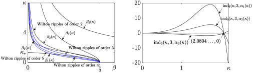
Figure 15. Left panel: domains of Wilton ripples of order $2$, $3$, $4$, and $5$; Right panel: graphs of ${\rm ind}_{9}(\kappa,3,\alpha_{i}(\kappa))$ (6.33) for $i=1,2,3$. We see ${\rm ind}_{9}(\kappa,3,\alpha_{1,2}(\kappa))>0$ when $0<\kappa<2.0804\ldots$ and ${\rm ind}_{9}(\kappa,3,\alpha_{3}(\kappa))>0$ when $\kappa>2.0804\ldots$.

We now discuss the expansions (6.23) for $j=5,6$. When $g_{1}$, $g_{2}$ are given by (6.30), in contrast to the case when they are given by (6.29), $g_{2}$ is a quadratic function of $\alpha$ for Wilton ripples of order $M\geqslant 3$. Specifically, when $M=3$,

$${\rm ind}_{10}(\kappa,3,\alpha)=a(\kappa,3)\alpha^{2}+b(\kappa,3)\alpha+c(\kappa,3)$$ (6.34)

and when $M\geqslant 4$,

$${\rm ind}_{10}(\kappa,M,\alpha)=a(\kappa,M)\alpha^{2}+c(\kappa,M).$$ (6.35)

That is the $\alpha$-order term does not appear in the formula of ${\rm ind}_{10}(\kappa,M,\alpha)$ for $M\geqslant 4$. When $M=3$, for we have found $\alpha$ takes the value of one of the real zeros of the cubic polynomial (2.20), it is feasible to investigate ${\rm ind}_{10}$ (6.34) at $(\kappa,3,\alpha_{i}(\kappa))$. For general $M\geqslant 4$, as we noted in Section 2.2.2, $\alpha$ is hard to obtain for large $M$. It is then unrealistic to fully investigate ${\rm ind}_{10}$ (6.35) at $(\kappa,M,\alpha_{i}(\kappa))$ for $i=1,\ldots,M$. However, since there is no $\alpha$-order term in (6.35), the sign of ${\rm ind}_{10}(\kappa,M,\alpha_{i}(\kappa))$ is independent of values of $\alpha_{i}(\kappa)$ provided that the sign of $a(\kappa,M)$ is the same as that of $c(\kappa,M)$. This perhaps is the most we can say about the expansions (6.23) for $j=5,6$ without knowing $\alpha$ for general Wilton ripple of order $M\geqslant 4$.

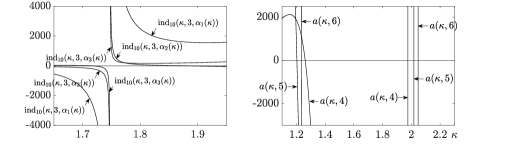
Figure 16. Left panel: graphs of ${\rm ind}_{10}(\kappa,3,\alpha_{i}(\kappa))$ (6.34) for $i=1,2,3$. We see ${\rm ind}_{10}(\kappa,3,\alpha_{1}(\kappa))>0$ when $1.8949\ldots<\kappa$, ${\rm ind}_{10}(\kappa,3,\alpha_{2}(\kappa))>0$ when $1.8949\ldots<\kappa<2.1443\ldots$, and ${\rm ind}_{10}(\kappa,3,\alpha_{3}(\kappa))>0$ when $0<\kappa<1.8313\ldots$ or $1.8949\ldots<\kappa$. The vertical asymptotic is at $\kappa=1.8949\ldots$ where $g_{1}$ (6.30) vanishes.

In FIGURE 16 left panel, we plot ${\rm ind}_{10}(\kappa,3,\alpha_{i}(\kappa))$ for $\alpha_{i}(\kappa)$ $i=1,2,3$ being the three real zeros of (2.20) in ascending order $\alpha_{1}(\kappa)<\alpha_{2}(\kappa)<0<\alpha_{3}(\kappa)$. The numerics show, for Wilton ripples of order $M=3$, the expansions (6.23), for $j=5,6$, bifurcate off the imaginary axis provided that

• $1.8949\ldots<\kappa$ when $\alpha$ takes the value $\alpha_{1}(\kappa)$,

• $1.8949\ldots<\kappa<2.1443\ldots$ when $\alpha$ takes the value $\alpha_{2}(\kappa)$,

• and $0<\kappa<1.8313\ldots$ or $1.8949\ldots<\kappa$ when $\alpha$ takes the value $\alpha_{3}(\kappa)$,

whence these waves are numerically found low-frequency unstable.

We numerically compute $a(\kappa,M)$ and $c(\kappa,M)$ in (6.35) for $M=4,5,6$ and find $c(\kappa,M)$ is positive. So ${\rm ind}_{10}>0$ provided that $a(\kappa,M)>0$. In FIGURE 16 right panel, we plot $a(\kappa,M)$ for $M=4,5,6$. The numerics show, without knowing the value of $\alpha$ in (LABEL:wiltonm_1) for Wilton ripples of order $M=4,5,6$, the expansions (6.23), for $j=5,6$, bifurcate off the imaginary axis provided that

• $\kappa<1.260\ldots$ or $1.975\ldots<\kappa$ when $M=4$,

• $\kappa<1.203\ldots$ or $2.018\ldots<\kappa$ when $M=5$,

• $\kappa<1.234\ldots$ or $2.047\ldots<\kappa$ when $M=6$,

whence these waves are numerically found low-frequency unstable.

Remark 12.

By continuity of the index function, for Wilton ripples of order $4$, ${\rm ind}_{10}(\kappa,M,\alpha)$ (6.35) shall be numerically found positive for waves with $\kappa$ slightly greater than $1.260\ldots$. However, as noted above, without knowing $\alpha$, one cannot find the critical $\kappa$’s where sign of (6.35) switches.

6.2.2. Wilton ripples of order $2$

We now turn to the discussion for Wilton ripples of order $2$. Because $\mu_{1}\neq 0$ (2.17), some entries of $\mathbf{a}^{(0,1)}$ are none-zero comparing to (6.19). This difference in the matrix $\mathbf{a}^{(0,1)}$ causes changes in the expansion of $\delta_{j}$, for $j=1,2$ (see (LABEL:expansion_wilton2)).

Lemma 6.14.

Computations show for Wilton ripples of order $2$

$$\mathbf{a}^{(0,1)}(T;0)=\begin{pmatrix}a^{(0,1)}_{11}&a^{(0,1)}_{11}&a^{(0,1)}_{13}&0&a^{(0,1)}_{15}&0\\ -a^{(0,1)}_{11}&-a^{(0,1)}_{11}&a^{(0,1)}_{13}&0&0&-a^{(0,1)}_{15}\\ 0&0&0&0&0&0\\ a^{(0,1)}_{41}&-a^{(0,1)}_{41}&a^{(0,1)}_{43}&0&a^{(0,1)}_{45}&-a^{(0,1)}_{45}\\ a^{(0,1)}_{51}&0&a^{(0,1)}_{53}&0&a^{(0,1)}_{55}&0\\ 0&-a^{(0,1)}_{51}&a^{(0,1)}_{53}&0&0&-a^{(0,1)}_{55}\end{pmatrix},$$ (6.36)

In particular, $a^{(0,1)}_{11}$, $a^{(0,1)}_{12}$, $a^{(0,1)}_{21}$, $a^{(0,1)}_{22}$, $a^{(0,1)}_{51}$, $a^{(0,1)}_{62}$, $a^{(0,1)}_{15}$, $a^{(0,1)}_{26}$, $a^{(0,1)}_{55}$, and $a^{(0,1)}_{66}$ are not zeros and formulas for entries $a^{(0,1)}_{11}$ and $a^{(0,1)}_{55}$ which will be used in Theorem 6.15 are given in Appendix G. Because $\mathbf{a}^{(0,0)}$, $\mathbf{a}^{(1,0)}$, and $\mathbf{a}^{(2,0)}$ are computed merely by the constant wave, we find (6.17), (6.18), and (6.27) also follow.

Proof.

$a^{(0,1)}_{11}(T)$ can be computed by

$$a^{(0,1)}_{11}(T)= e^{-i\kappa T}\Big{\langle}\int_{0}^{T}e^{i\kappa x}\mathbf{B}^{(0,1)}(x;0)e^{-i\kappa x}\boldsymbol{\phi}_{1}(0)~{}dx,\boldsymbol{\psi}_{1}(0)\Big{\rangle}$$

$$= \Big{\langle}\int_{0}^{T}\mathbf{B}^{(0,1)}(x;0)\boldsymbol{\phi}_{1}(0)~{}dx,\boldsymbol{\psi}_{1}(0)\Big{\rangle},$$

where $\mathbf{B}^{(0,1)}$ is given by (C.2), $\boldsymbol{\phi}_{1}(0)$ is given by (3.20), and $\boldsymbol{\psi}_{1}(0)$ is given by (3.44) with $j=1$. Terms in $\mathbf{B}^{(0,1)}(x;0)\boldsymbol{\phi}_{1}(0)$ (C.2) integrate to zero except for those containing $\mu_{1}$. Hence, $a^{(0,1)}_{11}(T)\neq 0$. Similar computation can be made for other entries. ∎

The periodic Evans function $\Delta(\delta,p\kappa+\gamma;\varepsilon)$ (3.9) can be expanded as

$$\Delta(\delta,p\kappa+\gamma;\varepsilon)= \sum_{l=0}^{6}d^{(l,6-l,0)}\delta^{l}\gamma^{6-l}+\sum_{l=0}^{6}d^{(l,6-l,1)}\delta^{l}\gamma^{6-l}\varepsilon$$ (6.37)

$$+\mathchoice{{\scriptstyle\mathcal{O}}}{{\scriptstyle\mathcal{O}}}{{\scriptscriptstyle\mathcal{O}}}{\scalebox{0.7}{$\scriptscriptstyle\mathcal{O}$}}((|\delta|+|\gamma|)^{6}+|\varepsilon|).$$

Again, the corresponding Weierstrass polynomial is $6$ order. Inserting

$$\delta_{j}(k_{j}(0)+\gamma,\varepsilon)=\delta^{(1,0)}_{j}\gamma+\delta^{(2,0)}_{j}\gamma^{2}+\delta^{(\frac{m}{s},\frac{n}{t})}_{j}\gamma^{\frac{m}{s}}\varepsilon^{\frac{n}{t}}+\cdots.$$

into (6.37), upon inspection, we obtain $\frac{m}{s}=1$ and $\frac{n}{t}=\frac{1}{2}$. Because $\delta^{(1,0)}_{j}$ $\delta^{(2,0)}_{j}$ can be computed merely by the constant wave, i.e., the dispersion relation, (6.26) also follows. To proceed, substituting

$$\delta_{j}(k_{j}(0)+\gamma,\varepsilon)$$ (6.38)

$$= \delta^{(1,0)}_{j}\gamma+\delta^{(2,0)}_{j}\gamma^{2}+\delta^{(1,\frac{1}{2})}_{j}\gamma\varepsilon^{\frac{1}{2}}+\cdots,\quad\text{for $j=1,2,5,6$,}$$

into (6.37) and evaluating at (6.26), the coefficient of $\gamma^{6}\varepsilon$ reads, for $j=1,2$,

$$-T^{4}(a^{(1,0)}_{11}-a^{(1,0)}_{55})^{2}\big{(}-(a^{(1,0)}_{11})^{2}+2a^{(1,0)}_{11}a^{(1,0)}_{33}$$ (6.39)

$$-(a^{(1,0)}_{33})^{2}+Ta^{(2,0)}_{34}\big{)}(a^{(1,0)}_{11})^{-6}\big{(}(a^{(1,0)}_{11})^{4}(\delta^{(1,\frac{1}{2})}_{j})^{2}$$

$$-Ta^{(0,1)}_{11}(T(a^{(1,0)}_{11})^{2}-2Ta^{(2,0)}_{11}+2a^{(1,0)}_{13}a^{(1,0)}_{41})\big{)}$$

and, for $j=5,6$,

$$-T^{4}(a^{(1,0)}_{11}-a^{(1,0)}_{55})^{2}\big{(}-(a^{(1,0)}_{33})^{2}+2a^{(1,0)}_{33}a^{(1,0)}_{55}$$ (6.40)

$$-(a^{(1,0)}_{55})^{2}+Ta^{(2,0)}_{34}\big{)}(a^{(1,0)}_{55})^{-6}\big{(}(a^{(1,0)}_{55})^{4}(\delta^{(1,\frac{1}{2})}_{j})^{2}$$

$$-Ta^{(0,1)}_{55}(T(a^{(1,0)}_{55})^{2}-2Ta^{(2,0)}_{55}+2a^{(1,0)}_{53}a^{(1,0)}_{45})\big{)}.$$

Theorem 6.15 (Spectral instability near $0\in\mathbb{C}$ at $\gamma\varepsilon^{\frac{1}{2}}$ order).

The $\kappa$-Wilton ripples of order $2$ of sufficiently small amplitude is spectrally unstable in the vicinity of $0\in\mathbb{C}$ provided that either

$${\rm ind}_{11}(\kappa)$$ (6.41)

$$:= a^{(0,1)}_{11}\big{(}T(a^{(1,0)}_{11})^{2}-2Ta^{(2,0)}_{11}+2a^{(1,0)}_{13}a^{(1,0)}_{41}\big{)}(a^{(1,0)}_{11})^{-4}$$

$$= -\kappa^{2}(4e^{2\kappa}+e^{4\kappa}+1)(42e^{2\kappa}+75e^{4\kappa}-212e^{6\kappa}+75e^{8\kappa}+42e^{10\kappa}$$

$$-11e^{12\kappa}+144\kappa^{2}e^{2\kappa}+144\kappa^{2}e^{4\kappa}+144\kappa^{2}e^{8\kappa}+144\kappa^{2}e^{10\kappa}$$

$$+120\kappa e^{2\kappa}+48\kappa e^{4\kappa}-48\kappa e^{8\kappa}-120\kappa e^{10\kappa}-11)$$

$$\cdot\big{(}1152\alpha\pi(e^{2\kappa}-1)^{2}(e^{2\kappa}+1)^{4}(e^{4\kappa}+1)\big{)}^{-1}$$

or

$${\rm ind}_{12}(\kappa)$$ (6.42)

$$:= a^{(0,1)}_{55}\big{(}T(a^{(1,0)}_{55})^{2}-2Ta^{(2,0)}_{55}+2a^{(1,0)}_{53}a^{(1,0)}_{45}\big{)}(a^{(1,0)}_{55})^{-4}$$

$$= -\kappa^{2}e^{-8\kappa}(4e^{2\kappa}+e^{4\kappa}+1)(32e^{2\kappa}+64e^{4\kappa}-32e^{6\kappa}$$

$$-82e^{8\kappa}-32e^{10\kappa}+64e^{12\kappa}+32e^{14\kappa}-23e^{16\kappa}+576\kappa^{2}e^{4\kappa}$$

$$-576\kappa^{2}e^{8\kappa}+576\kappa^{2}e^{12\kappa}+336\kappa e^{4\kappa}-384\kappa e^{6\kappa}+384\kappa e^{10\kappa}$$

$$-336\kappa e^{12\kappa}-23)\cdot\big{(}4608\alpha\pi\,{\rm sh}(4\kappa)^{2}(e^{4\kappa}+1)\big{)}^{-1},$$

where $\alpha$ is a root of (2.17), is positive.

Proof.

Solving (LABEL:eqn:g_wilton2_1) for $\delta^{(1,\frac{1}{2})}_{j}$, $j=1,2$ yields $(\delta^{(1,\frac{1}{2})}_{j})^{2}={\rm ind}_{11}(\kappa)T$. Hence, the expansion (LABEL:expansion_wilton2), for $j=1,2$, bifurcates off the imaginary axis provided that ${\rm ind}_{11}(\kappa)>0$. Similar argument can be made for $j=5,6$. ∎

Notice that the factor $\alpha$ appearing in the denominator of ${\rm ind}_{11}(\kappa)$ is given by one of the two roots of (2.17). Because the two roots have opposite sign, if the $\kappa$-wave with $\alpha=(8\,{\rm ch}(2\kappa))^{-\frac{1}{2}}$ is stable at the $\gamma\varepsilon^{\frac{1}{2}}$ order, the $\kappa$-wave with $\alpha=-(8\,{\rm ch}(2\kappa))^{-\frac{1}{2}}$ must be unstable at $\gamma\varepsilon^{\frac{1}{2}}$ order and vice versa. Furthermore, notice that the factor $\big{(}T(a^{(1,0)}_{11})^{2}-2Ta^{(2,0)}_{11}+2a^{(1,0)}_{13}a^{(1,0)}_{41}\big{)}$ in ${\rm ind}_{11}(\kappa)$ (LABEL:def:ind_11) also appears in $g_{2}$ (5.57) for capillary-gravity wave. Indeed, computation shows

$${\rm ind}_{11}(\kappa)=-\frac{\kappa^{2}(4e^{2\kappa}+e^{4\kappa}+1)^{3}}{288\alpha\pi(e^{2\kappa}-1)^{2}(e^{2\kappa}+1)^{6}(e^{4\kappa}+1)}{\rm ind}_{5,2}(\kappa)$$

where ${\rm ind}_{5,2}(\kappa)$ is given by evaluating ${\rm ind}_{5,2}(\beta,\kappa)$ (appearing in $\mathrm{ind}_{1}(\beta,\kappa)$ (5.58)) (E.2) on (LABEL:wilton_con) with $M=2$, the domain of Wilton ripples of order $2$. By the discussion 2 for the modulational stability diagram, ${\rm ind}_{5,2}(\beta,\kappa)$ is zero on the $\beta_{2}(\kappa)$-curve (see FIGURE 14 left panel). And the $\beta_{2}(\kappa)$-curve intersects the domain of Wilton ripples of order $2$, $\beta_{3}(\kappa)$-curve, at $(\beta_{*},\kappa_{*})=(0.19678\ldots,1.28523\ldots)$.

As for ${\rm ind}_{12}(\kappa)$, we can show by a computer-assisted proof, analogous to the proof of Lemma 2.1 that ${\rm ind}_{12}(\kappa)\alpha$ is always positive.

Let $(\beta_{*},\kappa_{*})=(0.19678\ldots,1.28523\ldots)$ be the point where the domain of Wilton ripples of order $2$, the $\beta_{3}(\kappa)$- curve, intersects the $\beta_{2}(\kappa)$- curve (see FIGURE 14 left panel). For the $\kappa$-wave with $\alpha=(8\,{\rm ch}(2\kappa))^{-\frac{1}{2}}$, the expansion (LABEL:expansion_wilton2), for $j=1,2$, is unstable at $\gamma\varepsilon^{\frac{1}{2}}$ order provided that $\kappa>\kappa_{*}$ and stable at $\gamma\varepsilon^{\frac{1}{2}}$ order provided that $\kappa<\kappa_{*}$. For the $\kappa$-wave with $\alpha=-(8\,{\rm ch}(2\kappa))^{-\frac{1}{2}}$, the expansion (LABEL:expansion_wilton2), for $j=1,2$, is stable at $\gamma\varepsilon^{\frac{1}{2}}$ order provided that $\kappa>\kappa_{*}$ and unstable at $\gamma\varepsilon^{\frac{1}{2}}$ order provided that $\kappa<\kappa_{*}$. For the $\kappa$-wave with $\alpha=(8\,{\rm ch}(2\kappa))^{-\frac{1}{2}}$, the expansion (LABEL:expansion_wilton2), for $j=5,6$, is always unstable at $\gamma\varepsilon^{\frac{1}{2}}$ order. For the $\kappa$-wave with $\alpha=-(8\,{\rm ch}(2\kappa))^{-\frac{1}{2}}$, the expansion (LABEL:expansion_wilton2), for $j=5,6$, is always stable at $\gamma\varepsilon^{\frac{1}{2}}$ order.

Appendix A Expansion for Wilton ripples

When $M=2$, at the order of $\varepsilon^{2}$, we collect

$$\begin{aligned} \phi_{2}(x,y)=&\alpha^{2}\kappa\,{\rm sh}(2\kappa)y\,{\rm s}(4\kappa x)\,{\rm sh}(2\kappa y)+\alpha\kappa\,{\rm sh}(\kappa)y\,{\rm s}(3\kappa x)\,{\rm sh}(2\kappa y)\\ &+\tfrac{1}{2}\alpha\kappa\,{\rm sh}(2\kappa)y\,{\rm s}(3\kappa x)\,{\rm sh}(\kappa y)+\tfrac{1}{2}\kappa\,{\rm sh}(\kappa)y\,{\rm s}(2\kappa x)\,{\rm sh}(\kappa y)\\ &+\alpha\kappa\,{\rm sh}(\kappa)y\,{\rm s}(\kappa x)\,{\rm sh}(2\kappa y)-\tfrac{1}{2}\alpha\kappa\,{\rm sh}(2\kappa)y\,{\rm s}(\kappa x)\,{\rm sh}(\kappa y)\\ &-\frac{\alpha^{2}\kappa(2\,{\rm ch}(4\kappa)-4\,{\rm ch}(2\kappa)+5)}{16\,{\rm sh}(\kappa)^{4}}\,{\rm s}(4\kappa x)\,{\rm ch}(4\kappa y)\\ &-\frac{\alpha\kappa(\,{\rm ch}(2\kappa)+9\,{\rm ch}(2\kappa)^{2}+8)}{4(\,{\rm ch}(2\kappa)-1)^{2}}\,{\rm s}(3\kappa x)\,{\rm ch}(3\kappa y)\\ &+c_{1}\,{\rm s}(2\kappa x)\,{\rm ch}(2\kappa y)-\alpha\kappa(2+3\,{\rm sh}(\kappa)^{2})\,{\rm s}(\kappa x)\,{\rm ch}(\kappa y),\\ \eta_{2}(x)=&-\frac{\alpha^{2}\kappa(4\,{\rm sh}(4\kappa)+\,{\rm sh}(8\kappa))}{8(\,{\rm ch}(2\kappa)-1)^{2}}\,{\rm c}(4\kappa x)\\ &-\frac{3\alpha\kappa(16\,{\rm ch}(2\kappa)+7\,{\rm ch}(4\kappa)+2\,{\rm ch}(6\kappa)+11)}{32\,{\rm sh}(\kappa)^{3}}\,{\rm c}(3\kappa x)\\ &+\tfrac{1}{4}\,{\rm sh}(2\kappa)(\kappa+4c_{1})\,{\rm c}(2\kappa x)\end{aligned}$$ (A.1)

where $c_{1}$ is determined upon solving (2.1a)-(2.1e) (2.2) at the order of $\varepsilon^{3}$. Solving at the order of $\varepsilon^{3}$, we obtain

$$\begin{aligned} c_{1}=&-\kappa(687\,{\rm sh}(\kappa)^{2}+2363\,{\rm sh}(\kappa)^{4}+4530\,{\rm sh}(\kappa)^{6}+4988\,{\rm sh}(\kappa)^{8}\\ &+3000\,{\rm sh}(\kappa)^{10}+768\,{\rm sh}(\kappa)^{12}+90)\\ &\cdot\big{(}128\,{\rm ch}(2\kappa)^{2}\,{\rm sh}(\kappa)^{4}(5\,{\rm sh}(\kappa)^{2}+2\,{\rm sh}(\kappa)^{4}+3)\big{)}^{-1},\\ \mu_{2}=&\kappa^{3}(\,{\rm ch}(2\kappa)+2)(16398\,{\rm ch}(2\kappa)+11611\,{\rm ch}(4\kappa)+6805\,{\rm ch}(6\kappa)\\ &+3002\,{\rm ch}(8\kappa)+1213\,{\rm ch}(10\kappa)+325\,{\rm ch}(12\kappa)+32\,{\rm ch}(14\kappa)\\ &+8998)\big{(}1536\,{\rm ch}(2\kappa)^{2}\,{\rm sh}(2\kappa)(\,{\rm ch}(2\kappa)-1)^{2}(\,{\rm ch}(2\kappa)+1)\\ &\cdot(2\,{\rm ch}(2\kappa)+1)\big{)}^{-1},\end{aligned}$$ (A.2)

and we omit the formulas for $\phi_{3},\;\eta_{3},\;q_{3}$. When $M\geqslant 3$, at the order of $\varepsilon^{2}$, we collect

$$\phi_{2}(x,y)$$ (A.3)

$$= \tfrac{1}{2}M\alpha^{2}\kappa\,{\rm sh}(M\kappa)y\,{\rm s}(2M\kappa x)\,{\rm sh}(M\kappa y)$$

$$+\tfrac{1}{2}M\alpha\kappa\,{\rm sh}(\kappa)y\,{\rm s}((M+1)\kappa x)\,{\rm sh}(M\kappa y)$$

$$+\tfrac{1}{2}\alpha\kappa\,{\rm sh}(M\kappa)y\,{\rm s}((M+1)\kappa x)\,{\rm sh}(\kappa y)$$

$$+\tfrac{1}{2}M\alpha\kappa\,{\rm sh}(\kappa)y\,{\rm s}((M-1)\kappa x)\,{\rm sh}(M\kappa y)$$

$$-\tfrac{1}{2}\alpha\kappa\,{\rm sh}(M\kappa)y\,{\rm s}((M-1)\kappa x)\,{\rm sh}(\kappa y)$$

$$+\tfrac{1}{2}\kappa\,{\rm sh}(\kappa)y\,{\rm s}(2\kappa x)\,{\rm sh}(\kappa y)$$

$$+3\alpha^{2}\kappa M(\,{\rm sh}(\kappa)-M^{2}\,{\rm sh}(\kappa)-2M^{2}\,{\rm ch}(M\kappa)^{2}\,{\rm sh}(\kappa)$$

$$+2M\,{\rm ch}(M\kappa)\,{\rm sh}(M\kappa)\,{\rm ch}(\kappa))\big{(}8(M^{2}\,{\rm sh}(\kappa)-\,{\rm sh}(\kappa)$$

$$+\,{\rm ch}(M\kappa)^{2}\,{\rm sh}(\kappa)+2M^{2}\,{\rm ch}(M\kappa)^{2}\,{\rm sh}(\kappa)$$

$$-3M\,{\rm ch}(M\kappa)\,{\rm sh}(M\kappa)\,{\rm ch}(\kappa))\big{)}^{-1}\,{\rm s}(2M\kappa x)\,{\rm ch}(2M\kappa y)$$

$$-\big{(}\alpha\kappa(3M-2\,{\rm ch}(2M\kappa)+3M^{3}\,{\rm ch}(2\kappa)+2M^{4}\,{\rm ch}(2\kappa)$$

$$-3M\,{\rm ch}(2M\kappa)-M^{3}\,{\rm ch}(2M\kappa)-3M^{3}-2M^{4}+M\,{\rm ch}(2\kappa)$$

$$+2M^{3}\,{\rm sh}(2\kappa)\,{\rm sh}(2M\kappa)-M\,{\rm ch}(2\kappa)\,{\rm ch}(2M\kappa)$$

$$-2M\,{\rm sh}(2\kappa)\,{\rm sh}(2M\kappa)+M^{3}\,{\rm ch}(2\kappa)\,{\rm ch}(2M\kappa)+2)\big{)}$$

$$\cdot\big{(}2(3M-2\,{\rm ch}(2M\kappa)+M^{2}\,{\rm ch}(2(M+1)\kappa)+3M^{2}\,{\rm ch}(2\kappa)$$

$$+2M^{3}\,{\rm ch}(2\kappa)-3M\,{\rm ch}(2M\kappa)-M\,{\rm ch}(2(M+1)\kappa)$$

$$-M^{2}\,{\rm ch}(2M\kappa)-3M^{2}-2M^{3}+M\,{\rm ch}(2\kappa)+2)\big{)}^{-1}$$

$$\cdot\,{\rm s}((M+1)\kappa x)\,{\rm ch}((M+1)\kappa y)$$

$$-\alpha\kappa\big{(}3M+2\,{\rm ch}(2M\kappa)+3M^{3}\,{\rm ch}(2\kappa)-2M^{4}\,{\rm ch}(2\kappa)$$

$$-3M\,{\rm ch}(2M\kappa)-M^{3}\,{\rm ch}(2M\kappa)-3M^{3}+2M^{4}+M\,{\rm ch}(2\kappa)$$

$$-2M^{3}\,{\rm sh}(2\kappa)\,{\rm sh}(2M\kappa)-M\,{\rm ch}(2\kappa)\,{\rm ch}(2M\kappa)$$

$$+2M\,{\rm sh}(2\kappa)\,{\rm sh}(2M\kappa)+M^{3}\,{\rm ch}(2\kappa)\,{\rm ch}(2M\kappa)-2\big{)}$$

$$\cdot\big{(}2(3M+2\,{\rm ch}(2M\kappa)-M^{2}c(2(M-1))-3M^{2}\,{\rm ch}(2\kappa)$$

$$+2M^{3}\,{\rm ch}(2\kappa)-3M\,{\rm ch}(2M\kappa)-Mc(2(M-1))$$

$$+M^{2}\,{\rm ch}(2M\kappa)+3M^{2}-2M^{3}+M\,{\rm ch}(2\kappa)-2)\big{)}^{-1}$$

$$\cdot\,{\rm s}((M-1)\kappa x)\,{\rm ch}((M-1)\kappa y)$$

$$-3\kappa(2\,{\rm sh}(M\kappa)+\,{\rm ch}(2\kappa)\,{\rm sh}(M\kappa)-M^{2}\,{\rm sh}(M\kappa)$$

$$-M\,{\rm sh}(2\kappa)\,{\rm ch}(M\kappa))\big{(}4(4\,{\rm sh}(M\kappa)+2\,{\rm ch}(2\kappa)\,{\rm sh}(M\kappa)$$

$$-M^{2}\,{\rm sh}(M\kappa)+M^{2}\,{\rm ch}(2\kappa)\,{\rm sh}(M\kappa)-3M\,{\rm sh}(2\kappa)\,{\rm ch}(M\kappa))\big{)}^{-1}$$

$$\cdot\,{\rm s}(2\kappa x)\,{\rm ch}(2\kappa y)$$

$$\eta_{2}(x)$$ (A.4)

$$= -\alpha^{2}\kappa M\,{\rm ch}(M\kappa)\,{\rm sh}(M\kappa)\,{\rm sh}(\kappa)(M^{2}-1)(\,{\rm ch}(2M\kappa)+2)$$

$$\cdot\big{(}4(M^{2}\,{\rm sh}(\kappa)-\,{\rm sh}(\kappa)+\,{\rm ch}(M\kappa)^{2}\,{\rm sh}(\kappa)+2M^{2}\,{\rm ch}(M\kappa)^{2}\,{\rm sh}(\kappa)$$

$$-3M\,{\rm ch}(M\kappa)\,{\rm sh}(M\kappa)\,{\rm ch}(\kappa))\big{)}^{-1}\,{\rm c}(2M\kappa x)$$

$$-2\alpha\kappa(M^{2}-1)\big{(}\,{\rm ch}(M\kappa)^{3}\,{\rm sh}(\kappa)-\,{\rm ch}(M\kappa)\,{\rm sh}(\kappa)$$

$$+M^{2}\,{\rm sh}(M\kappa)\,{\rm ch}(\kappa)^{3}-M^{2}\,{\rm sh}(M\kappa)\,{\rm ch}(\kappa)$$

$$-2M\,{\rm ch}(M\kappa)^{2}\,{\rm sh}(M\kappa)\,{\rm ch}(\kappa)-2M\,{\rm ch}(M\kappa)\,{\rm ch}(\kappa)^{2}\,{\rm sh}(\kappa)$$

$$+2M\,{\rm ch}(M\kappa)^{2}\,{\rm sh}(M\kappa)\,{\rm ch}(\kappa)^{3}+2M\,{\rm ch}(M\kappa)^{3}\,{\rm ch}(\kappa)^{2}\,{\rm sh}(\kappa)\big{)}$$

$$\cdot\big{(}3M-2\,{\rm ch}(2M\kappa)+M^{2}\,{\rm ch}(2(M+1)\kappa)+3M^{2}\,{\rm ch}(2\kappa)$$

$$+2M^{3}\,{\rm ch}(2\kappa)-3M\,{\rm ch}(2M\kappa)-M\,{\rm ch}(2(M+1)\kappa)$$

$$-M^{2}\,{\rm ch}(2M\kappa)-3M^{2}-2M^{3}+M\,{\rm ch}(2\kappa)+2\big{)}^{-1}\,{\rm c}((M+1)\kappa x)$$

$$-2\alpha\kappa(M^{2}-1)\big{(}\,{\rm ch}(M\kappa)^{3}\,{\rm sh}(\kappa)-\,{\rm ch}(M\kappa)\,{\rm sh}(\kappa)$$

$$-M^{2}\,{\rm sh}(M\kappa)\,{\rm ch}(\kappa)^{3}+M^{2}\,{\rm sh}(M\kappa)\,{\rm ch}(\kappa)$$

$$-2M\,{\rm ch}(M\kappa)^{2}\,{\rm sh}(M\kappa)\,{\rm ch}(\kappa)+2M\,{\rm ch}(M\kappa)\,{\rm ch}(\kappa)^{2}\,{\rm sh}(\kappa)$$

$$+2M\,{\rm ch}(M\kappa)^{2}\,{\rm sh}(M\kappa)\,{\rm ch}(\kappa)^{3}-2M\,{\rm ch}(M\kappa)^{3}\,{\rm ch}(\kappa)^{2}\,{\rm sh}(\kappa)\big{)}$$

$$\cdot\big{(}3M+2\,{\rm ch}(2M\kappa)-M^{2}\,{\rm ch}(2(M-1)\kappa)-3M^{2}\,{\rm ch}(2\kappa)$$

$$+2M^{3}\,{\rm ch}(2\kappa)-3M\,{\rm ch}(2M\kappa)-M\,{\rm ch}(2(M-1)\kappa)$$

$$+M^{2}\,{\rm ch}(2M\kappa)+3M^{2}-2M^{3}+M\,{\rm ch}(2\kappa)-2\big{)}^{-1}\,{\rm c}((M-1)\kappa x)$$

$$+\kappa\,{\rm sh}(M\kappa)\,{\rm ch}(\kappa)\,{\rm sh}(\kappa)(M^{2}-1)(2\,{\rm ch}(\kappa)^{2}+1)\big{(}4\,{\rm sh}(M\kappa)$$

$$+8\,{\rm sh}(M\kappa)\,{\rm ch}(\kappa)^{2}-4M^{2}\,{\rm sh}(M\kappa)+4M^{2}\,{\rm sh}(M\kappa)\,{\rm ch}(\kappa)^{2}$$

$$-12M\,{\rm ch}(M\kappa)\,{\rm ch}(\kappa)\,{\rm sh}(\kappa)\big{)}^{-1}\,{\rm c}(2\kappa x).$$

Solving at the order of $\varepsilon^{3}$, we obtain $q_{3}=0$ and, for $M\geqslant 4$,

$$\mu_{2}(\kappa,M,\alpha)=\mu_{2,2}(\kappa,M)\alpha^{2}+\mu_{2,0}(\kappa,M)$$ (A.5)

where $\mu_{2,0}(\kappa,M)$ is given by (2.13) evaluated at $\beta=\beta(\kappa,M)$ (LABEL:wilton_con) and $\mu_{2,2}(\kappa,M)$ is given by

$$\mu_{2,2}(\kappa,M)=$$ (A.6)

$$M^{2}\Big{(}-2\kappa^{3}M^{10}\,{\rm sh}(M\kappa)\,{\rm sh}(\kappa)^{5}(\,{\rm sh}(\kappa)^{2}+1)-\kappa^{3}M^{9}\,{\rm ch}(M\kappa)\,{\rm ch}(\kappa)$$

$$\cdot(\,{\rm ch}(\kappa)^{2}-1)^{2}(\,{\rm ch}(M\kappa)^{2}\,{\rm ch}(\kappa)^{2}-5\,{\rm ch}(\kappa)^{2}+2\,{\rm ch}(M\kappa)^{4}\,{\rm ch}(\kappa)^{2}$$

$$+\,{\rm ch}(M\kappa)^{2}+1)+\kappa^{3}M^{8}\,{\rm sh}(M\kappa)\,{\rm sh}(\kappa)^{3}(2\,{\rm sh}(M\kappa)^{2}-12\,{\rm sh}(M\kappa)^{4}$$

$$+16\,{\rm sh}(\kappa)^{2}+15\,{\rm sh}(\kappa)^{4}+23\,{\rm sh}(M\kappa)^{2}\,{\rm sh}(\kappa)^{2}+20\,{\rm sh}(M\kappa)^{2}\,{\rm sh}(\kappa)^{4}$$

$$-14\,{\rm sh}(M\kappa)^{4}\,{\rm sh}(\kappa)^{2}-2\,{\rm sh}(M\kappa)^{4}\,{\rm sh}(\kappa)^{4})-\kappa^{3}M^{7}\,{\rm ch}(M\kappa)\,{\rm ch}(\kappa)$$

$$\cdot(\,{\rm ch}(\kappa)^{2}-1)(16\,{\rm ch}(\kappa)^{2}-34\,{\rm ch}(\kappa)^{4}-37\,{\rm ch}(M\kappa)^{2}\,{\rm ch}(\kappa)^{2}$$

$$+73\,{\rm ch}(M\kappa)^{2}\,{\rm ch}(\kappa)^{4}-29\,{\rm ch}(M\kappa)^{4}\,{\rm ch}(\kappa)^{4}+\,{\rm ch}(M\kappa)^{6}\,{\rm ch}(\kappa)^{2}$$

$$-2\,{\rm ch}(M\kappa)^{2}+9\,{\rm ch}(M\kappa)^{4}+\,{\rm ch}(M\kappa)^{6}+2)-\kappa^{3}M^{6}\,{\rm sh}(M\kappa)\,{\rm sh}(\kappa)$$

$$\cdot(14\,{\rm sh}(\kappa)^{4}-16\,{\rm sh}(M\kappa)^{6}+6\,{\rm sh}(\kappa)^{6}+30\,{\rm sh}(M\kappa)^{2}\,{\rm sh}(\kappa)^{2}$$

$$+103\,{\rm sh}(M\kappa)^{2}\,{\rm sh}(\kappa)^{4}+23\,{\rm sh}(M\kappa)^{4}\,{\rm sh}(\kappa)^{2}+61\,{\rm sh}(M\kappa)^{2}\,{\rm sh}(\kappa)^{6}$$

$$+84\,{\rm sh}(M\kappa)^{4}\,{\rm sh}(\kappa)^{4}-31\,{\rm sh}(M\kappa)^{6}\,{\rm sh}(\kappa)^{2}+56\,{\rm sh}(M\kappa)^{4}\,{\rm sh}(\kappa)^{6}$$

$$-14\,{\rm sh}(M\kappa)^{6}\,{\rm sh}(\kappa)^{4})-2\kappa^{3}M^{5}\,{\rm ch}(M\kappa)\,{\rm ch}(\kappa)(12\,{\rm ch}(\kappa)^{2}-17\,{\rm ch}(\kappa)^{4}$$

$$+\,{\rm ch}(\kappa)^{6}+7\,{\rm ch}(M\kappa)^{2}\,{\rm ch}(\kappa)^{4}-7\,{\rm ch}(M\kappa)^{4}\,{\rm ch}(\kappa)^{2}+17\,{\rm ch}(M\kappa)^{2}\,{\rm ch}(\kappa)^{6}$$

$$-17\,{\rm ch}(M\kappa)^{6}\,{\rm ch}(\kappa)^{2}-22\,{\rm ch}(M\kappa)^{4}\,{\rm ch}(\kappa)^{6}+22\,{\rm ch}(M\kappa)^{6}\,{\rm ch}(\kappa)^{4}$$

$$-12\,{\rm ch}(M\kappa)^{2}+17\,{\rm ch}(M\kappa)^{4}-\,{\rm ch}(M\kappa)^{6})+\kappa^{3}M^{4}\,{\rm sh}(M\kappa)\,{\rm sh}(\kappa)$$

$$\cdot(14\,{\rm sh}(M\kappa)^{4}+6\,{\rm sh}(M\kappa)^{6}-16\,{\rm sh}(\kappa)^{6}+30\,{\rm sh}(M\kappa)^{2}\,{\rm sh}(\kappa)^{2}$$

$$+23\,{\rm sh}(M\kappa)^{2}\,{\rm sh}(\kappa)^{4}+103\,{\rm sh}(M\kappa)^{4}\,{\rm sh}(\kappa)^{2}-31\,{\rm sh}(M\kappa)^{2}\,{\rm sh}(\kappa)^{6}$$

$$+84\,{\rm sh}(M\kappa)^{4}\,{\rm sh}(\kappa)^{4}+61\,{\rm sh}(M\kappa)^{6}\,{\rm sh}(\kappa)^{2}-14\,{\rm sh}(M\kappa)^{4}\,{\rm sh}(\kappa)^{6}$$

$$+56\,{\rm sh}(M\kappa)^{6}\,{\rm sh}(\kappa)^{4})+\kappa^{3}M^{3}\,{\rm ch}(M\kappa)\,{\rm ch}(\kappa)(\,{\rm ch}(M\kappa)^{2}-1)$$

$$\cdot(9\,{\rm ch}(\kappa)^{4}-2\,{\rm ch}(\kappa)^{2}+\,{\rm ch}(\kappa)^{6}-37\,{\rm ch}(M\kappa)^{2}\,{\rm ch}(\kappa)^{2}$$

$$+73\,{\rm ch}(M\kappa)^{4}\,{\rm ch}(\kappa)^{2}+\,{\rm ch}(M\kappa)^{2}\,{\rm ch}(\kappa)^{6}-29\,{\rm ch}(M\kappa)^{4}\,{\rm ch}(\kappa)^{4}$$

$$+16\,{\rm ch}(M\kappa)^{2}-34\,{\rm ch}(M\kappa)^{4}+2)-\kappa^{3}M^{2}\,{\rm sh}(M\kappa)^{3}\,{\rm sh}(\kappa)$$

$$\cdot(16\,{\rm sh}(M\kappa)^{2}+15\,{\rm sh}(M\kappa)^{4}+2\,{\rm sh}(\kappa)^{2}-12\,{\rm sh}(\kappa)^{4}+23\,{\rm sh}(M\kappa)^{2}\,{\rm sh}(\kappa)^{2}$$

$$-14\,{\rm sh}(M\kappa)^{2}\,{\rm sh}(\kappa)^{4}+20\,{\rm sh}(M\kappa)^{4}\,{\rm sh}(\kappa)^{2}-2\,{\rm sh}(M\kappa)^{4}\,{\rm sh}(\kappa)^{4})$$

$$+\kappa^{3}M\,{\rm ch}(M\kappa)\,{\rm ch}(\kappa)(\,{\rm ch}(M\kappa)^{2}-1)^{2}(\,{\rm ch}(\kappa)^{2}+\,{\rm ch}(M\kappa)^{2}\,{\rm ch}(\kappa)^{2}$$

$$+2\,{\rm ch}(M\kappa)^{2}\,{\rm ch}(\kappa)^{4}-5\,{\rm ch}(M\kappa)^{2}+1)+2\kappa^{3}\,{\rm sh}(M\kappa)^{5}\,{\rm sh}(\kappa)$$

$$\cdot(\,{\rm sh}(M\kappa)^{2}+1)\Big{)}\cdot\Big{(}4\,{\rm ch}(\kappa)(M^{2}-1)^{2}(\,{\rm ch}(\kappa)^{2}-1)\big{(}-M^{6}(\,{\rm sh}(M\kappa)$$

$$-2\,{\rm sh}(M\kappa)\,{\rm ch}(\kappa)^{2}+\,{\rm sh}(M\kappa)\,{\rm ch}(\kappa)^{4})+M^{5}(2\,{\rm ch}(M\kappa)\,{\rm ch}(\kappa)^{3}\,{\rm sh}(\kappa)$$

$$+2\,{\rm ch}(M\kappa)^{3}\,{\rm ch}(\kappa)\,{\rm sh}(\kappa)-2\,{\rm ch}(M\kappa)^{3}\,{\rm ch}(\kappa)^{3}\,{\rm sh}(\kappa)$$

$$-2\,{\rm ch}(M\kappa)\,{\rm ch}(\kappa)\,{\rm sh}(\kappa))-M^{4}(2\,{\rm sh}(M\kappa)\,{\rm ch}(\kappa)^{2}-\,{\rm ch}(M\kappa)^{4}\,{\rm sh}(M\kappa)$$

$$-3\,{\rm sh}(M\kappa)+\,{\rm sh}(M\kappa)\,{\rm ch}(\kappa)^{4}+5\,{\rm ch}(M\kappa)^{2}\,{\rm sh}(M\kappa)\,{\rm ch}(\kappa)^{2}$$

$$-5\,{\rm ch}(M\kappa)^{2}\,{\rm sh}(M\kappa)\,{\rm ch}(\kappa)^{4}+\,{\rm ch}(M\kappa)^{4}\,{\rm sh}(M\kappa)\,{\rm ch}(\kappa)^{2})$$

$$+M^{3}(4\,{\rm ch}(M\kappa)\,{\rm ch}(\kappa)^{3}\,{\rm sh}(\kappa)-4\,{\rm ch}(M\kappa)^{3}\,{\rm ch}(\kappa)\,{\rm sh}(\kappa)$$

$$+4\,{\rm ch}(M\kappa)^{5}\,{\rm ch}(\kappa)\,{\rm sh}(\kappa)-4\,{\rm ch}(M\kappa)^{3}\,{\rm ch}(\kappa)^{3}\,{\rm sh}(\kappa))$$

$$+M^{2}(2\,{\rm ch}(M\kappa)^{2}\,{\rm sh}(M\kappa)-3\,{\rm sh}(M\kappa)+\,{\rm ch}(M\kappa)^{4}\,{\rm sh}(M\kappa)$$

$$-\,{\rm sh}(M\kappa)\,{\rm ch}(\kappa)^{4}+5\,{\rm ch}(M\kappa)^{2}\,{\rm sh}(M\kappa)\,{\rm ch}(\kappa)^{2}+\,{\rm ch}(M\kappa)^{2}\,{\rm sh}(M\kappa)\,{\rm ch}(\kappa)^{4}$$

$$-5\,{\rm ch}(M\kappa)^{4}\,{\rm sh}(M\kappa)\,{\rm ch}(\kappa)^{2})+M(2\,{\rm ch}(M\kappa)^{5}\,{\rm ch}(\kappa)\,{\rm sh}(\kappa)$$

$$-4\,{\rm ch}(M\kappa)^{3}\,{\rm ch}(\kappa)\,{\rm sh}(\kappa)+2\,{\rm ch}(M\kappa)\,{\rm ch}(\kappa)\,{\rm sh}(\kappa))+\,{\rm sh}(M\kappa)$$

$$-2\,{\rm ch}(M\kappa)^{2}\,{\rm sh}(M\kappa)+\,{\rm ch}(M\kappa)^{4}\,{\rm sh}(M\kappa)\big{)}\Big{)}^{-1}.$$

And, for $M=3$, there is an additional $\alpha$-order term in the formula of $\mu_{2}(\kappa,3,\alpha)$, namely,

$$\mu_{2}(\kappa,3,\alpha)=\mu_{2,2}(\kappa,3)\alpha^{2}+\mu_{2,1}(\kappa)\alpha+\mu_{2,0}(\kappa,3),$$ (A.7)

where

$$\mu_{2,1}(\kappa)= -3\kappa^{3}\,{\rm ch}(\kappa)^{3}\big{(}108\,{\rm ch}(\kappa)^{6}-18\,{\rm ch}(\kappa)^{4}+351\,{\rm ch}(\kappa)^{8}$$

$$-4194\,{\rm ch}(\kappa)^{10}+8856\,{\rm ch}(\kappa)^{12}\big{)}$$

$$\cdot\big{(}8\,{\rm sh}(\kappa)^{5}(4\,{\rm sh}(\kappa)^{2}+3)^{2}(6\,{\rm sh}(\kappa)^{2}+7)\big{)}^{-1}.$$

We omit the formulas for $\phi_{3},\;\eta_{3},\;\ldots$.

Appendix B Proof of Lemma 3.3

Let $\lambda\in{\rm spec}(\mathcal{L}(\varepsilon))$, and suppose that $\mathbf{u}=\begin{pmatrix}\phi\\ u\\ \eta\\ z\end{pmatrix}\in L^{\infty}(\mathbb{R};Y)$, by abuse of notation, is a nontrivial solution of (3.2) satisfying $\mathbf{u}(x+T)=e^{ikT}\mathbf{u}(x)$ for all $x\in\mathbb{R}$ for some $k\in\mathbb{R}$. Notice that (3.2) remains invariant under

$$\lambda\mapsto\lambda^{*}\quad\text{and}\quad\mathbf{u}\mapsto\mathbf{u}^{*},$$

and $\mathbf{u}^{*}(x+T)=e^{-ikT}\mathbf{u}^{*}(x)$ for all $x\in\mathbb{R}$, where the asterisk denotes complex conjugation. Thus $\lambda^{*}\in{\rm spec}(\mathcal{L}(\varepsilon))$. Also, notice that (3.2) remains invariant under

$$\lambda\mapsto-\lambda\quad\text{and}\quad\begin{pmatrix}\phi(x)\\ u(x)\\ \eta(x)\\ z(x)\end{pmatrix}\mapsto\begin{pmatrix}-\phi(-x)\\ u(-x)\\ \eta(-x)\\ -z(-x)\end{pmatrix}=:\mathbf{u}_{-}(x),$$

and $\mathbf{u}_{-}(x+T)=e^{-ikT}\mathbf{u}_{-}(x)$ for all $x\in\mathbb{R}$. Thus $-\lambda\in{\rm spec}(\mathcal{L}(\varepsilon))$. This completes the proof.

Appendix C Expansion of $\mathbf{B}(x;\sigma,\delta,\epsilon)$

Throughout the section, let $\mathbf{u}=\begin{pmatrix}\phi\\ u\\ \eta\\ z\end{pmatrix}$. Recalling (3.54), we use (2.2), (3.2), (3.3), (3.6), (3.7), (3.8), (3.8), (3.9), and make straightforward calculations to show that

$$\mathbf{B}^{(1,0)}(x;\sigma)\mathbf{u} =\begin{pmatrix}-y^{2}z/(2\beta)\\ -\eta\\ 0\\ (\phi(1)+i\sigma\eta)/\mu_{0}\end{pmatrix}\quad\text{and}$$ (C.1)

$$\mathbf{B}^{(2,0)}(x;\sigma)\mathbf{u} =\begin{pmatrix}0\\ 0\\ 0\\ \eta/(2\mu_{0})\end{pmatrix}.$$

Notice that $\mathbf{B}^{(m,0)}$, $m\geqslant 1$, do not involve $x$.

Let $\mathbf{B}^{(0,1)}(x;\sigma)\mathbf{u}=\begin{pmatrix}(\mathbf{B}^{(0,1)}(x;\sigma)\mathbf{u})_{1}\\ (\mathbf{B}^{(0,1)}(x;\sigma)\mathbf{u})_{2}\\ (\mathbf{B}^{(0,1)}(x;\sigma)\mathbf{u})_{3}\\ (\mathbf{B}^{(0,1)}(x;\sigma)\mathbf{u})_{4}\end{pmatrix}$, and we make straightforward calculations to show that

$$\begin{aligned} (\mathbf{B}^{(0,1)}(x;\sigma)\mathbf{u})_{1}&=\left({\phi_{1}}_{xx}(1)-2{\eta_{1}}_{x}\right)\phi+2y{\eta_{1}}_{x}\phi_{y}+{\eta_{1}}_{x}\phi(0)\\ &\quad+\left({\phi_{1}}_{x}(1)-\eta_{1}\right)u-{\eta_{1}}_{xx}\int_{0}^{y}y^{\prime}u(y^{\prime})dy^{\prime}\\ &\quad+\tfrac{2i\sigma y^{2}{\eta_{1}}_{x}-y^{2}{\phi_{1}}_{xy}(1)}{2}\eta+\tfrac{2y{\phi_{1}}_{y}-y^{2}{\phi_{1}}_{y}(1)-i\sigma y^{2}{\phi_{1}}_{x}(1)}{2\beta}z,\\ (\mathbf{B}^{(0,1)}(x;\sigma)\mathbf{u})_{2}&=\left({\phi_{1}}_{x}(1)+\eta_{1}\right)\phi_{yy}-{\eta_{1}}_{x}u+\tfrac{y{\phi_{1}}_{xy}}{\beta}z\\ &\quad+\left(i\sigma\eta_{1}-{\phi_{1}}_{y}(1)+2{\phi_{1}}_{yy}\right)\eta,\\ (\mathbf{B}^{(0,1)}(x;\sigma)\mathbf{u})_{3}&=0,\\ (\mathbf{B}^{(0,1)}(x;\sigma)\mathbf{u})_{4}&=-\tfrac{i\sigma(\mu_{0}{\phi_{1}}_{x}(1)-\mu_{0}\eta_{1}+\mu_{1})}{\mu_{0}^{2}}\phi(1)+\tfrac{\mu_{0}{\phi_{1}}_{x}(1)+\mu_{1}}{\mu_{0}^{2}}u(1)\\ &\quad+\tfrac{i\sigma{\eta_{1}}_{x}}{\mu_{0}}\int_{0}^{1}yu(y)dy+\tfrac{\sigma(i\mu_{0}{\phi_{1}}_{y}(1)-\sigma\mu_{0}\eta_{1}+\mu_{1}\sigma)}{2\mu_{0}^{2}}\eta\\ &\quad+\tfrac{-{\phi_{1}}_{y}(1)}{\beta\mu_{0}}z,\end{aligned}$$ (C.2)

where $$\phi_{1} \eta_{1}$$ and are in (2.4), and, likewise,

$$\begin{aligned} (\mathbf{B}^{(1,1)}(x;\sigma)\mathbf{u})_{1}&=y^{2}{\eta_{1}}_{x}\eta-\tfrac{y^{2}{\phi_{1}}_{x}(1)}{2\beta}z,\\ (\mathbf{B}^{(1,1)}(x;\sigma)\mathbf{u})_{2}&=\eta_{1}\eta,\\ (\mathbf{B}^{(1,1)}(x;\sigma)\mathbf{u})_{3}&=0,\\ (\mathbf{B}^{(1,1)}(x;\sigma)\mathbf{u})_{4}&=\tfrac{\mu_{0}\eta_{1}-\mu_{0}{\phi_{1}}_{x}(1)-\mu_{1}}{\mu_{0}^{2}}\phi(1)+\tfrac{{\eta_{1}}_{x}}{\mu_{0}}\int_{0}^{1}yu(y)dy\\ &\quad+\tfrac{\mu_{0}{\phi_{1}}_{y}(1)-2i\sigma\mu_{1}+2i\mu_{0}\sigma\eta_{1}}{2\mu_{0}^{2}}\eta.\end{aligned}$$ (C.3)

Additionally, we calculate that

$$(\mathbf{B}^{(0,2)}(x;\sigma)\mathbf{u})_{1}$$ (C.4)

$$= +\big{(}{\phi_{2}}_{xx}(1)-{\phi_{1}}_{y}(1){\eta_{1}}_{xx}-3{\eta_{1}}_{x}{\eta_{1}}_{xx}-2{\eta_{2}}_{x}-{\phi_{1}}_{xy}(1){\eta_{1}}_{x}$$

$$+{\phi_{1}}_{x}(1){\phi_{1}}_{xx}(1)+2\eta_{1}{\eta_{1}}_{x}\big{)}\phi+\left(2y{\eta_{2}}_{x}-2y\eta_{1}{\eta_{1}}_{x}\right)\phi_{y}$$

$$+\left({\eta_{2}}_{x}-\eta_{1}{\eta_{1}}_{x}\right)\phi(0)+\big{(}{\phi_{2}}_{x}(1)-\eta_{2}-{\phi_{1}}_{x}(1)\eta_{1}-3{\eta_{1}}_{x}^{2}/2$$

$$+{\phi_{1}}_{x}(1)^{2}+\eta_{1}^{2}+y^{2}{\eta_{1}}_{x}^{2}-{\phi_{1}}_{y}(1){\eta_{1}}_{x}\big{)}u$$

$$+\left(-{\phi_{1}}_{x}(1){\eta_{1}}_{xx}-{\eta_{2}}_{xx}\right)\int_{0}^{y}y^{\prime}u(y^{\prime})dy^{\prime}$$

$$+\big{(}2\phi_{1}{\eta_{1}}_{x}-y^{2}{\phi_{2}}_{xy}(1)/2-2{\eta_{1}}_{x}\phi_{1}(\cdot,0)+i\sigma y^{2}{\eta_{2}}_{x}-3y{\phi_{1}}_{y}{\eta_{1}}_{x}$$

$$-y^{2}{\phi_{1}}_{x}(1){\phi_{1}}_{xy}(1)/2+2y^{2}{\phi_{1}}_{y}(1){\eta_{1}}_{x}+y^{2}\eta_{1}{\phi_{1}}_{xy}(1)$$

$$+i\sigma y^{2}{\phi_{1}}_{x}(1){\eta_{1}}_{x}-i\sigma y^{2}\eta_{1}{\eta_{1}}_{x}\big{)}\eta+\Big{(}y{\phi_{2}}_{y}-y^{2}{\phi_{2}}_{y}(1)/2$$

$$-\int_{0}^{y}{y^{\prime}}^{2}{\phi_{1}}_{xy^{\prime}}dy^{\prime}{\eta_{1}}_{x}-i\sigma y^{2}{\phi_{2}}_{x}(1)/2+y{\phi_{1}}_{x}(1){\phi_{1}}_{y}-2y\eta_{1}{\phi_{1}}_{y}$$

$$-i\sigma y^{2}{\phi_{1}}_{x}(1)^{2}/2-y^{2}{\phi_{1}}_{x}(1){\phi_{1}}_{y}(1)/2+y^{2}{\phi_{1}}_{y}(1)\eta_{1}$$

$$+i\sigma y^{2}{\phi_{1}}_{y}(1){\eta_{1}}_{x}/2\Big{)}z/\beta,$$

$$(\mathbf{B}^{(0,2)}(x;\sigma)\mathbf{u})_{2}$$

$$= \left({\phi_{2}}_{x}(1)+\eta_{2}-{\phi_{1}}_{x}(1)\eta_{1}-3{\eta_{1}}_{x}^{2}/2-\eta_{1}^{2}-{\phi_{1}}_{y}(1){\eta_{1}}_{x}\right)\phi_{yy}$$

$$+\left(\eta_{1}{\eta_{1}}_{x}-{\eta_{2}}_{x}\right)u+\big{(}3{\phi_{1}}_{y}(1)\eta_{1}-i\sigma\eta_{1}^{2}-{\phi_{2}}_{y}(1)+i\sigma\eta_{2}$$

$$-6\eta_{1}{\phi_{1}}_{yy}-y{\eta_{1}}_{x}{\phi_{1}}_{xy}+2{\phi_{2}}_{yy}\big{)}\eta$$

$$+\big{(}y{\phi_{2}}_{xy}-y\eta_{1}{\phi_{1}}_{xy}-y^{2}{\eta_{1}}_{x}{\phi_{1}}_{yy}-y{\phi_{1}}_{y}{\eta_{1}}_{x}\big{)}z/\beta,$$

$$(\mathbf{B}^{(0,2)}(x;\sigma)\mathbf{u})_{3}=3{\eta_{1}}_{x}^{2}z/(2\beta),$$

$$(\mathbf{B}^{(0,2)}(x;\sigma)\mathbf{u})_{4}$$

$$= i\big{(}\mu_{1}^{2}\sigma-\mu_{0}^{2}\sigma{\phi_{2}}_{x}(1)+\mu_{0}^{2}\sigma\eta_{2}-\mu_{0}\mu_{2}\sigma+3\mu_{0}^{2}\sigma{\eta_{1}}_{x}^{2}/2+\mu_{0}^{2}\sigma{\phi_{1}}_{y}(1){\eta_{1}}_{x}$$

$$-\mu_{0}^{2}\sigma{\phi_{1}}_{x}(1)\eta_{1}+\mu_{0}\mu_{1}\sigma{\phi_{1}}_{x}(1)-\mu_{0}\mu_{1}\sigma\eta_{1}\big{)}\mu_{0}^{-3}\phi(1)$$

$$+\left(\mu_{0}^{2}{\phi_{2}}_{x}(1)+\mu_{0}\mu_{2}-\mu_{1}^{2}-\mu_{0}\mu_{1}{\phi_{1}}_{x}(1)\right)\mu_{0}^{-3}u(1)$$

$$+i\sigma\big{(}\mu_{0}{\eta_{2}}_{x}-\mu_{1}{\eta_{1}}_{x}+\mu_{0}\eta_{1}{\eta_{1}}_{x}\big{)}\mu_{0}^{-2}\int_{0}^{1}yu(y)dy$$

$$+\big{(}\mu_{0}\mu_{2}\sigma^{2}-\mu_{1}^{2}\sigma^{2}+i\sigma\mu_{0}^{2}{\phi_{2}}_{y}(1)-\mu_{0}^{2}\sigma^{2}\eta_{2}-i\sigma\mu_{0}^{2}{\phi_{1}}_{y}(1)\eta_{1}$$

$$-i\sigma\mu_{0}\mu_{1}{\phi_{1}}_{y}(1)+\mu_{0}\mu_{1}\sigma^{2}\eta_{1}\big{)}\mu_{0}^{-3}\eta/2+\big{(}\mu_{1}{\phi_{1}}_{y}(1)-\mu_{0}{\phi_{2}}_{y}(1)$$

$$+\mu_{0}{\phi_{1}}_{x}(1){\phi_{1}}_{y}(1)+\mu_{0}{\phi_{1}}_{y}(1)\eta_{1}\big{)}\mu_{0}^{-2}\beta^{-1}z.$$

We do not include the formulas of $\mathbf{B}^{(m,n)}(\sigma)$, $m+n\geqslant 3$.

Appendix D $\mathbf{a}^{(m,n)}$ for non-resonant capillary-gravity waves

$$\begin{aligned} a^{(1,0)}_{11}&=\frac{-4\pi\,{\rm sh}(2\kappa)(\beta\kappa^{2}+1)}{\kappa(2\kappa-\,{\rm sh}(2\kappa)+2\beta\kappa^{3}+\beta\kappa^{2}\,{\rm sh}(2\kappa))},\\ a^{(1,0)}_{13}&=\frac{4i\pi\,{\rm sh}(\kappa)(\beta\kappa^{2}+1)}{\kappa^{2}(2\kappa-\,{\rm sh}(2\kappa)+2\beta\kappa^{3}+\beta\kappa^{2}\,{\rm sh}(2\kappa))},\\ a^{(1,0)}_{33}&=\frac{2\pi\,{\rm sh}(\kappa)(\beta\kappa^{2}+1)}{\kappa(\,{\rm sh}(\kappa)-\kappa\,{\rm ch}(\kappa)+\beta\kappa^{2}\,{\rm sh}(\kappa))},\\ a^{(1,0)}_{41}&=\frac{-2\pi\,{\rm ch}(\kappa)\,{\rm sh}(\kappa)}{\kappa\,{\rm sh}(\kappa)-\kappa^{2}\,{\rm ch}(\kappa)+\beta\kappa^{3}\,{\rm sh}(\kappa)},\end{aligned}$$ (D.1)

$$\begin{aligned} a^{(0,1)}_{13}&=\frac{-2\pi\,{\rm sh}(\kappa)(\beta\kappa^{2}+1)(2\,{\rm sh}(\kappa)^{2}+\beta\kappa^{2}+3)}{\,{\rm ch}(\kappa)(2\kappa-\,{\rm sh}(2\kappa)+2\beta\kappa^{3}+\beta\kappa^{2}\,{\rm sh}(2\kappa))},\\ a^{(0,1)}_{41}&=-i\pi(4\,{\rm ch}(\kappa)-4\,{\rm ch}(\kappa)^{3}+\kappa\,{\rm sh}(\kappa)+\beta\kappa^{3}\,{\rm sh}(\kappa)\\ &\quad+2\kappa\,{\rm ch}(\kappa)^{2}\,{\rm sh}(\kappa))\big{(}\,{\rm sh}(\kappa)-\kappa\,{\rm ch}(\kappa)+\beta\kappa^{2}\,{\rm sh}(\kappa)\big{)}^{-1},\end{aligned}$$ (D.2)

$$\begin{aligned} a^{(2,0)}_{11}&=\frac{{a^{(1,0)}_{11}}^{2}}{2}+4i\pi\,{\rm sh}(2\kappa)e^{2\kappa}(\beta\kappa^{2}+1)\big{(}-\kappa^{5}(e^{2\kappa}-1)(6e^{4\kappa}\\ &\quad-3e^{8\kappa}+16\kappa^{2}e^{2\kappa}-16\kappa^{2}e^{4\kappa}+16\kappa^{2}e^{6\kappa}+24\kappa e^{2\kappa}-24\kappa e^{6\kappa}\\ &\quad-3)\beta^{3}-\kappa^{3}(3\kappa-10e^{2\kappa}-20e^{4\kappa}+20e^{6\kappa}+10e^{8\kappa}-10e^{10\kappa}\\ &\quad-72\kappa^{2}e^{2\kappa}-16\kappa^{3}e^{2\kappa}+88\kappa^{2}e^{4\kappa}-88\kappa^{2}e^{6\kappa}+72\kappa^{2}e^{8\kappa}\\ &\quad-16\kappa^{3}e^{8\kappa}-61\kappa e^{2\kappa}+58\kappa e^{4\kappa}+58\kappa e^{6\kappa}-61\kappa e^{8\kappa}+3\kappa e^{10\kappa}\\ &\quad+10)\beta^{2}-\kappa(6\kappa-3e^{2\kappa}-6e^{4\kappa}+6e^{6\kappa}+3e^{8\kappa}-3e^{10\kappa}\\ &\quad-80\kappa^{2}e^{2\kappa}-32\kappa^{3}e^{2\kappa}+96\kappa^{2}e^{4\kappa}-96\kappa^{2}e^{6\kappa}+80\kappa^{2}e^{8\kappa}\end{aligned}$$ (D.3)

$$-32\kappa^{3}e^{8\kappa}-34\kappa e^{2\kappa}+28\kappa e^{4\kappa}+28\kappa e^{6\kappa}-34\kappa e^{8\kappa}$$

$$\quad+6\kappa e^{10\kappa}+3)\beta+e^{2\kappa}-2e^{4\kappa}-2e^{6\kappa}+e^{8\kappa}+e^{10\kappa}+16\kappa^{2}e^{2\kappa}$$

$$\quad+16\kappa^{2}e^{8\kappa}+24\kappa e^{2\kappa}-40\kappa e^{4\kappa}+40\kappa e^{6\kappa}-24\kappa e^{8\kappa}+1\big{)}$$

$$\quad\cdot\big{(}\kappa(\kappa-e^{2\kappa}+\beta\kappa^{2}+\kappa e^{2\kappa}-\beta\kappa^{2}e^{2\kappa}+1)(4\kappa e^{2\kappa}-\beta\kappa^{2}$$

$$\quad-e^{4\kappa}+4\beta\kappa^{3}e^{2\kappa}+\beta\kappa^{2}e^{4\kappa}+1)^{3}\big{)}^{-1},$$

$$a^{(2,0)}_{34} =\frac{2\pi(e^{4\kappa}-1)(\beta\kappa^{2}+1)}{(\kappa-e^{2\kappa}+\beta\kappa^{2}+\kappa e^{2\kappa}-\beta\kappa^{2}e^{2\kappa}+1)^{2}},$$

$$\begin{aligned} a^{(1,1)}_{31}&=-i\pi\,{\rm sh}(2\kappa)(\beta\kappa^{2}+1)\big{(}3\kappa-4e^{2\kappa}+4e^{6\kappa}-2e^{8\kappa}-2\kappa^{2}e^{2\kappa}\\ &\quad+8\kappa^{3}e^{4\kappa}+2\kappa^{2}e^{6\kappa}+6\beta\kappa^{2}+\beta\kappa^{3}-8\kappa e^{2\kappa}+10\kappa e^{4\kappa}\\ &\quad-8\kappa e^{6\kappa}+3\kappa e^{8\kappa}-12\beta\kappa^{2}e^{2\kappa}-8\beta\kappa^{3}e^{2\kappa}-6\beta\kappa^{4}e^{2\kappa}\\ &\quad+14\beta\kappa^{3}e^{4\kappa}+12\beta\kappa^{2}e^{6\kappa}-8\beta\kappa^{3}e^{6\kappa}+8\beta\kappa^{5}e^{4\kappa}-6\beta\kappa^{2}e^{8\kappa}\\ &\quad+6\beta\kappa^{4}e^{6\kappa}+\beta\kappa^{3}e^{8\kappa}+2\big{)}\cdot\big{(}(\kappa-e^{2\kappa}+\beta\kappa^{2}+\kappa e^{2\kappa}\\ &\quad-\beta\kappa^{2}e^{2\kappa}+1)^{2}\cdot(4\kappa e^{2\kappa}-\beta\kappa^{2}-e^{4\kappa}+4\beta\kappa^{3}e^{2\kappa}\\ &\quad+\beta\kappa^{2}e^{4\kappa}+1)\big{)}^{-1},\\ a^{(1,1)}_{14}&=2\pi(e^{2\kappa}-1)(\beta\kappa^{2}+1)^{2}(e^{4\kappa}+2\kappa e^{2\kappa}-1)\big{(}\kappa-e^{2\kappa}-e^{4\kappa}\\ &\quad+e^{6\kappa}+4\kappa^{2}e^{2\kappa}+4\kappa^{2}e^{4\kappa}-\beta\kappa^{3}-\beta^{2}\kappa^{4}+5\kappa e^{2\kappa}-5\kappa e^{4\kappa}\\ &\quad-\kappa e^{6\kappa}+\beta^{2}\kappa^{4}e^{2\kappa}+4\beta^{2}\kappa^{5}e^{2\kappa}+\beta^{2}\kappa^{4}e^{4\kappa}-4\beta^{2}\kappa^{5}e^{4\kappa}\\ &\quad-\beta^{2}\kappa^{4}e^{6\kappa}+7\beta\kappa^{3}e^{2\kappa}+4\beta\kappa^{4}e^{2\kappa}-7\beta\kappa^{3}e^{4\kappa}+4\beta\kappa^{4}e^{4\kappa}\\ &\quad+\beta\kappa^{3}e^{6\kappa}+1\big{)}^{-1},\end{aligned}$$ (D.4)

$$\begin{aligned} a^{(0,2)}_{11}&=-i\kappa\pi(e^{2\kappa}-1)\big{(}2\kappa^{6}(4e^{2\kappa}+e^{4\kappa}+1)(\kappa-32e^{2\kappa}+64e^{4\kappa}\\ &\quad-32e^{6\kappa}+32\kappa^{2}e^{4\kappa}-6\kappa e^{2\kappa}+6\kappa e^{6\kappa}-\kappa e^{8\kappa})\beta^{3}\\ &\quad+\kappa^{4}(1216e^{6\kappa}-224e^{2\kappa}-352e^{4\kappa}-13\kappa-352e^{8\kappa}\\ &\quad-224e^{10\kappa}-32e^{12\kappa}+64\kappa^{2}e^{2\kappa}+430\kappa^{2}e^{4\kappa}+1120\kappa^{2}e^{6\kappa}\\ &\quad+430\kappa^{2}e^{8\kappa}+64\kappa^{2}e^{10\kappa}+2\kappa^{2}e^{12\kappa}+2\kappa^{2}-72\kappa e^{2\kappa}\\ &\quad-153\kappa e^{4\kappa}+153\kappa e^{8\kappa}+72\kappa e^{10\kappa}+13\kappa e^{12\kappa}-32)\beta^{2}\\ &\quad+\kappa^{2}(\kappa-160e^{2\kappa}-368e^{4\kappa}+1088e^{6\kappa}-368e^{8\kappa}-160e^{10\kappa}\\ &\quad-16e^{12\kappa}+62\kappa^{2}e^{2\kappa}+479\kappa^{2}e^{4\kappa}+1220\kappa^{2}e^{6\kappa}+479\kappa^{2}e^{8\kappa}\\ &\quad+62\kappa^{2}e^{10\kappa}+\kappa^{2}e^{12\kappa}+\kappa^{2}-36\kappa e^{2\kappa}-75\kappa e^{4\kappa}+75\kappa e^{8\kappa}\\ &\quad+36\kappa e^{10\kappa}-\kappa e^{12\kappa}-16)\beta+16\kappa-144e^{4\kappa}+256e^{6\kappa}\\ &\quad-144e^{8\kappa}+16e^{12\kappa}+16\kappa^{2}e^{2\kappa}+104\kappa^{2}e^{4\kappa}+320\kappa^{2}e^{6\kappa}\end{aligned}$$ (D.5)

$$\quad+104\kappa^{2}e^{8\kappa}+16\kappa^{2}e^{10\kappa}+8\kappa^{2}e^{12\kappa}+8\kappa^{2}+32\kappa e^{2\kappa}+32\kappa e^{4\kappa}$$

$$\quad-32\kappa e^{8\kappa}-32\kappa e^{10\kappa}-16\kappa e^{12\kappa}+16\big{)}\cdot\big{(}32\kappa^{6}e^{2\kappa}(e^{4\kappa}+4\kappa e^{2\kappa}$$

$$\quad-1)(3e^{2\kappa}-3e^{4\kappa}-e^{6\kappa}+1)\beta^{3}+16\kappa^{4}e^{2\kappa}(2e^{4\kappa}-3e^{2\kappa}-2\kappa$$

$$\quad+2e^{6\kappa}-3e^{8\kappa}+e^{10\kappa}+8\kappa^{2}e^{2\kappa}+40\kappa^{2}e^{4\kappa}+40\kappa^{2}e^{6\kappa}+8\kappa^{2}e^{8\kappa}$$

$$\quad+2\kappa e^{2\kappa}+52\kappa e^{4\kappa}-52\kappa e^{6\kappa}-2\kappa e^{8\kappa}+2\kappa e^{10\kappa}+1)\beta^{2}$$

$$\quad+16\kappa^{2}e^{2\kappa}(3\kappa+6e^{2\kappa}-8e^{4\kappa}-8e^{6\kappa}+6e^{8\kappa}+2e^{10\kappa}+4\kappa^{2}e^{2\kappa}$$

$$\quad+44\kappa^{2}e^{4\kappa}+44\kappa^{2}e^{6\kappa}+4\kappa^{2}e^{8\kappa}+9\kappa e^{2\kappa}+54\kappa e^{4\kappa}-54\kappa e^{6\kappa}$$

$$\quad-9\kappa e^{8\kappa}-3\kappa e^{10\kappa}+2)\beta-16e^{2\kappa}(e^{2\kappa}-1)^{2}(\kappa-e^{2\kappa}-e^{4\kappa}+e^{6\kappa}$$

$$\quad+4\kappa^{2}e^{2\kappa}+4\kappa^{2}e^{4\kappa}+5\kappa e^{2\kappa}-5\kappa e^{4\kappa}-\kappa e^{6\kappa}+1)\big{)}^{-1}.$$

Appendix E Modulational stability indices

Substitute (D.1), (D.2), (D.3), (D.4), and (D.5) in (5.57), after simplification, we find

$$\begin{aligned} g_{1}&=\frac{4\pi^{2}(e^{2\kappa}-1)(\beta\kappa^{2}+1)}{\kappa^{2}\#_{1}^{2}\#_{2}}{\rm ind}_{5,1},\\ g_{2}&=\frac{\kappa\pi}{256e^{4\kappa}\,{\rm sh}(2\kappa)(e^{2\kappa}+1)(\beta\kappa^{2}+1)^{2}\#_{1}^{2}\#_{2}}\frac{{\rm ind}_{5,2}{\rm ind}_{5,3}}{{\rm ind}_{5,4}},\\ \end{aligned}$$ (E.1)

where

$$\begin{aligned} &{\rm ind}_{5,1}\\ =&\kappa^{4}(3e^{4\kappa}+4\kappa e^{2\kappa}-3)^{2}\beta^{2}+2\kappa^{2}(2\kappa-6e^{4\kappa}+3e^{8\kappa}+16\kappa^{2}e^{4\kappa}\\ &-12\kappa e^{2\kappa}+12\kappa e^{6\kappa}-2\kappa e^{8\kappa}+3)\beta+4\kappa-2e^{4\kappa}+e^{8\kappa}\\ &+16\kappa^{2}e^{4\kappa}-4\kappa e^{8\kappa}+1,\\ &{\rm ind}_{5,2}\\ =&\kappa^{4}(6e^{4\kappa}-3e^{8\kappa}+16\kappa^{2}e^{2\kappa}-16\kappa^{2}e^{4\kappa}+16\kappa^{2}e^{6\kappa}+24\kappa e^{2\kappa}\\ &-24\kappa e^{6\kappa}-3)\beta^{2}+2\kappa^{2}(6e^{4\kappa}-3e^{8\kappa}+16\kappa^{2}e^{2\kappa}-16\kappa^{2}e^{4\kappa}\\ &+16\kappa^{2}e^{6\kappa}+16\kappa e^{2\kappa}-16\kappa e^{6\kappa}-3)\beta+e^{8\kappa}-2e^{4\kappa}+16\kappa^{2}e^{2\kappa}\\ &-16\kappa^{2}e^{4\kappa}+16\kappa^{2}e^{6\kappa}+8\kappa e^{2\kappa}-8\kappa e^{6\kappa}+1,\end{aligned}$$ (E.2)

$${\rm ind}_{5,3}$$

$$= 2\kappa^{8}(4e^{2\kappa}+e^{4\kappa}+1)(42e^{2\kappa}-9e^{4\kappa}-84e^{6\kappa}-9e^{8\kappa}+42e^{10\kappa}$$

$$+9e^{12\kappa}+16\kappa^{2}e^{4\kappa}+416\kappa^{2}e^{6\kappa}+16\kappa^{2}e^{8\kappa}-24\kappa e^{2\kappa}-240\kappa e^{4\kappa}$$

$$+240\kappa e^{8\kappa}+24\kappa e^{10\kappa}+9)\beta^{4}+\kappa^{6}(8\kappa-188e^{2\kappa}-28e^{4\kappa}+188e^{6\kappa}$$

$$+142e^{8\kappa}+188e^{10\kappa}-28e^{12\kappa}-188e^{14\kappa}-43e^{16\kappa}+80\kappa^{2}e^{4\kappa}$$

$$+2880\kappa^{2}e^{6\kappa}+12512\kappa^{2}e^{8\kappa}+2880\kappa^{2}e^{10\kappa}+80\kappa^{2}e^{12\kappa}+168\kappa e^{2\kappa}$$

$$-112\kappa e^{4\kappa}-3384\kappa e^{6\kappa}+3384\kappa e^{10\kappa}+112\kappa e^{12\kappa}-168\kappa e^{14\kappa}$$

$$-8\kappa e^{16\kappa}-43)\beta^{3}+4\kappa^{4}(3\kappa-135e^{2\kappa}-314e^{4\kappa}+135e^{6\kappa}+636e^{8\kappa}$$

$$+135e^{10\kappa}-314e^{12\kappa}-135e^{14\kappa}-4e^{16\kappa}+48\kappa^{2}e^{4\kappa}+720\kappa^{2}e^{6\kappa}$$

$$+4224\kappa^{2}e^{8\kappa}+720\kappa^{2}e^{10\kappa}+48\kappa^{2}e^{12\kappa}+66\kappa e^{2\kappa}+498\kappa e^{4\kappa}$$

$$+138\kappa e^{6\kappa}-138\kappa e^{10\kappa}-498\kappa e^{12\kappa}-66\kappa e^{14\kappa}-3\kappa e^{16\kappa}-4)\beta^{2}$$

$$+\kappa^{2}(36\kappa-132e^{2\kappa}-892e^{4\kappa}+132e^{6\kappa}+1686e^{8\kappa}+132e^{10\kappa}$$

$$-892e^{12\kappa}-132e^{14\kappa}+49e^{16\kappa}+272\kappa^{2}e^{4\kappa}+960\kappa^{2}e^{6\kappa}+9824\kappa^{2}e^{8\kappa}$$

$$+960\kappa^{2}e^{10\kappa}+272\kappa^{2}e^{12\kappa}+48\kappa e^{2\kappa}+1560\kappa e^{4\kappa}+2736\kappa e^{6\kappa}$$

$$-2736\kappa e^{10\kappa}-1560\kappa e^{12\kappa}-48\kappa e^{14\kappa}-36\kappa e^{16\kappa}+49)\beta+32\kappa$$

$$+64e^{2\kappa}-144e^{4\kappa}-64e^{6\kappa}+208e^{8\kappa}-64e^{10\kappa}-144e^{12\kappa}$$

$$+64e^{14\kappa}+40e^{16\kappa}+128\kappa^{2}e^{4\kappa}+2048\kappa^{2}e^{8\kappa}+128\kappa^{2}e^{12\kappa}+128\kappa e^{4\kappa}$$

$$+768\kappa e^{6\kappa}-768\kappa e^{10\kappa}-128\kappa e^{12\kappa}-32\kappa e^{16\kappa}+40,$$

$${\rm ind}_{5,4}$$

$$= -2\kappa^{2}(4e^{2\kappa}+e^{4\kappa}+1)\beta+(e^{2\kappa}-1)^{2},$$

and

$$\#_{1} =4\kappa e^{2\kappa}-\beta\kappa^{2}-e^{4\kappa}+4\beta\kappa^{3}e^{2\kappa}+\beta\kappa^{2}e^{4\kappa}+1,$$

$$\#_{2} =\kappa-e^{2\kappa}+\beta\kappa^{2}+\kappa e^{2\kappa}-\beta\kappa^{2}e^{2\kappa}+1.$$

Appendix F $\mathbf{a}^{(m,n)}$ for Wilton ripples of order $\geqslant 3$

The left upper $4$ by $4$ block matrices of $\mathbf{a}^{(1,0)}$ and $\mathbf{a}^{(2,0)}$ are given by evaluating (D.1) (D.3) at the domain of Wilton ripples of order $M$ (LABEL:wilton_con). Furthermore,

$$\begin{aligned} a_{45}^{(1,0)}&=-\frac{\pi e^{-2\kappa}(4e^{2\kappa}-4e^{6\kappa}-e^{8\kappa}+1)}{\kappa(2\kappa-3e^{4\kappa}+8\kappa e^{2\kappa}+2\kappa e^{4\kappa}+3)},\\ a_{53}^{(1,0)}&=\frac{6i\pi e^{2\kappa}(e^{4\kappa}-1)}{\kappa^{2}(8e^{2\kappa}-8e^{6\kappa}+e^{8\kappa}+24\kappa e^{4\kappa}-1)},\\ a_{55}^{(1,0)}&=-\frac{12\pi(e^{8\kappa}-1)}{\kappa(8e^{2\kappa}-8e^{6\kappa}+e^{8\kappa}+24\kappa e^{4\kappa}-1)},\end{aligned}$$ (F.1)

$$\begin{aligned} &a_{13}^{(0,1)}\\ =&-\pi(M^{2}-1)(\,{\rm sh}(\kappa)-M^{2}\,{\rm sh}(\kappa)-\,{\rm ch}(M\kappa)^{2}\,{\rm sh}(\kappa)\\ &+M^{2}\,{\rm ch}(M\kappa)^{2}\,{\rm sh}(\kappa)-2M^{2}\,{\rm ch}(\kappa)^{2}\,{\rm sh}(\kappa)\\ &+2M^{2}\,{\rm ch}(M\kappa)^{2}\,{\rm ch}(\kappa)^{2}\,{\rm sh}(\kappa)-2M\,{\rm ch}(M\kappa)\,{\rm sh}(M\kappa)\,{\rm ch}(\kappa)^{3}\\ &+2M\,{\rm ch}(M\kappa)\,{\rm sh}(M\kappa)\,{\rm ch}(\kappa))\big{(}M(\,{\rm ch}(M\kappa)\,{\rm sh}(\kappa)\\ &-M\,{\rm sh}(M\kappa)\,{\rm ch}(\kappa))(\kappa\,{\rm sh}(M\kappa)-\kappa M^{2}\,{\rm sh}(M\kappa)\\ &-2M\,{\rm ch}(M\kappa)\,{\rm sh}(\kappa)^{2}+\,{\rm sh}(M\kappa)\,{\rm ch}(\kappa)\,{\rm sh}(\kappa)\\ &+M^{2}\,{\rm sh}(M\kappa)\,{\rm ch}(\kappa)\,{\rm sh}(\kappa))\big{)}^{-1},\\ &a_{41}^{(0,1)}\\ =&4i\pi\alpha M\,{\rm sh}(\kappa)(-M\,{\rm ch}(\kappa)\,{\rm ch}(M\kappa)^{2}+\,{\rm sh}(M\kappa)\,{\rm sh}(\kappa)\,{\rm ch}(M\kappa)\\ &+M\,{\rm ch}(\kappa))\big{(}\,{\rm sh}(M\kappa)\,{\rm sh}(\kappa)-M^{2}\,{\rm sh}(M\kappa)\,{\rm sh}(\kappa)\\ &+\kappa M^{2}\,{\rm sh}(M\kappa)\,{\rm ch}(\kappa)-\kappa M\,{\rm ch}(M\kappa)\,{\rm sh}(\kappa)\big{)}^{-1}\\ &-i\pi\,{\rm sh}(\kappa)(4M\,{\rm ch}(M\kappa)+\kappa\,{\rm sh}(M\kappa)-\kappa M^{2}\,{\rm sh}(M\kappa)\\ &-4M\,{\rm ch}(M\kappa)\,{\rm ch}(\kappa)^{2}-2\kappa M^{2}\,{\rm sh}(M\kappa)\,{\rm ch}(\kappa)^{2}\\ &+4M^{2}\,{\rm sh}(M\kappa)\,{\rm ch}(\kappa)\,{\rm sh}(\kappa)+2\kappa M\,{\rm ch}(M\kappa)\,{\rm ch}(\kappa)\,{\rm sh}(\kappa))\\ &\cdot\big{(}\,{\rm sh}(M\kappa)\,{\rm sh}(\kappa)-M^{2}\,{\rm sh}(M\kappa)\,{\rm sh}(\kappa)+\kappa M^{2}\,{\rm sh}(M\kappa)\,{\rm ch}(\kappa)\\ &-\kappa M\,{\rm ch}(M\kappa)\,{\rm sh}(\kappa)\big{)}^{-1},\\ &a_{43}^{(0,1)}\\ =&-2\pi\alpha\Big{(}(\,{\rm sh}(M\kappa)-\kappa M\,{\rm ch}(M\kappa))\kappa^{-1}+\,{\rm sh}(M\kappa)(\,{\rm sh}(M\kappa)\,{\rm sh}(\kappa)\\ &-M^{2}\,{\rm sh}(M\kappa)\,{\rm sh}(\kappa)-\kappa M^{2}\,{\rm sh}(M\kappa)\,{\rm ch}(\kappa)+\kappa M\,{\rm ch}(M\kappa)\,{\rm sh}(\kappa))\\ &\quad\cdot\big{(}\kappa(\,{\rm sh}(M\kappa)\,{\rm sh}(\kappa)-M^{2}\,{\rm sh}(M\kappa)\,{\rm sh}(\kappa)+\kappa M^{2}\,{\rm sh}(M\kappa)\,{\rm ch}(\kappa)\\ &-\kappa M\,{\rm ch}(M\kappa)\,{\rm sh}(\kappa))\big{)}^{-1}\Big{)}-2\pi(\,{\rm sh}(\kappa)-\kappa\,{\rm ch}(\kappa))\kappa^{-1}\\ &-2\pi\,{\rm sh}(\kappa)(\,{\rm sh}(M\kappa)\,{\rm sh}(\kappa)-M^{2}\,{\rm sh}(M\kappa)\,{\rm sh}(\kappa)\\ &-\kappa M^{2}\,{\rm sh}(M\kappa)\,{\rm ch}(\kappa)+\kappa M\,{\rm ch}(M\kappa)\,{\rm sh}(\kappa))\big{(}\kappa(\,{\rm sh}(M\kappa)\,{\rm sh}(\kappa)\\ &-M^{2}\,{\rm sh}(M\kappa)\,{\rm sh}(\kappa)+\kappa M^{2}\,{\rm sh}(M\kappa)\,{\rm ch}(\kappa)-\kappa M\,{\rm ch}(M\kappa)\,{\rm sh}(\kappa))\big{)}^{-1},\\ &a_{45}^{(0,1)}\\ =&4i\pi M\,{\rm sh}(M\kappa)\,{\rm sh}(\kappa)(\,{\rm ch}(M\kappa)\,{\rm sh}(\kappa)-M\,{\rm sh}(M\kappa)\,{\rm ch}(\kappa))\\ &\cdot\big{(}\,{\rm sh}(M\kappa)\,{\rm sh}(\kappa)-M^{2}\,{\rm sh}(M\kappa)\,{\rm sh}(\kappa)+\kappa M^{2}\,{\rm sh}(M\kappa)\,{\rm ch}(\kappa)\\ &-\kappa M\,{\rm ch}(M\kappa)\,{\rm sh}(\kappa)\big{)}^{-1}-i\pi\alpha M(4\,{\rm ch}(M\kappa)\,{\rm sh}(\kappa)\\ &-4\,{\rm ch}(M\kappa)^{3}\,{\rm sh}(\kappa)+4M\,{\rm sh}(M\kappa)^{3}\,{\rm ch}(\kappa)+2\kappa M^{2}\,{\rm ch}(M\kappa)\,{\rm ch}(\kappa)\\ &+2\kappa M\,{\rm sh}(M\kappa)^{3}\,{\rm sh}(\kappa)-\kappa M^{3}\,{\rm sh}(M\kappa)\,{\rm sh}(\kappa)\\ &-2\kappa M^{2}\,{\rm ch}(M\kappa)^{3}\,{\rm ch}(\kappa)+3\kappa M\,{\rm sh}(M\kappa)\,{\rm sh}(\kappa))\big{(}\,{\rm sh}(M\kappa)\,{\rm sh}(\kappa)\\ &\quad-M^{2}\,{\rm sh}(M\kappa)\,{\rm sh}(\kappa)+\kappa M^{2}\,{\rm sh}(M\kappa)\,{\rm ch}(\kappa)-\kappa M\,{\rm ch}(M\kappa)\,{\rm sh}(\kappa)\big{)}^{-1},\end{aligned}$$ (F.2)

$$a_{53}^{(0,1)}$$

$$= \alpha M\pi(M^{2}-1)(\,{\rm sh}(M\kappa)+2\,{\rm ch}(M\kappa)^{2}\,{\rm sh}(M\kappa)-\,{\rm sh}(M\kappa)\,{\rm ch}(\kappa)^{2}$$

$$-M^{2}\,{\rm sh}(M\kappa)+M^{2}\,{\rm sh}(M\kappa)\,{\rm ch}(\kappa)^{2}-2\,{\rm ch}(M\kappa)^{2}\,{\rm sh}(M\kappa)\,{\rm ch}(\kappa)^{2}$$

$$-2M\,{\rm ch}(M\kappa)\,{\rm ch}(\kappa)\,{\rm sh}(\kappa)+2M\,{\rm ch}(M\kappa)^{3}\,{\rm ch}(\kappa)\,{\rm sh}(\kappa))$$

$$\cdot\big{(}(\,{\rm ch}(M\kappa)\,{\rm sh}(\kappa)-M\,{\rm sh}(M\kappa)\,{\rm ch}(\kappa))(\kappa M^{3}\,{\rm sh}(\kappa)-\kappa M\,{\rm sh}(\kappa)$$

$$+\,{\rm ch}(M\kappa)\,{\rm sh}(M\kappa)\,{\rm sh}(\kappa)-2M\,{\rm sh}(M\kappa)^{2}\,{\rm ch}(\kappa)$$

$$+M^{2}\,{\rm ch}(M\kappa)\,{\rm sh}(M\kappa)\,{\rm sh}(2\kappa))\big{)}^{-1}.$$

Appendix G $\mathbf{a}^{(m,n)}$ for Wilton ripples of order $2$

$$\begin{aligned} a_{11}^{(0,1)}&=-\frac{3i\kappa\pi\,{\rm sh}(2\kappa)(5e^{2\kappa}+5e^{4\kappa}+e^{6\kappa}+1)}{4\alpha\,{\rm ch}(2\kappa)(9e^{2\kappa}-9e^{4\kappa}-e^{6\kappa}+12\kappa e^{2\kappa}+12\kappa e^{4\kappa}+1)},\\ a_{55}^{(0,1)}&=\frac{3i\kappa\pi(4e^{2\kappa}-4e^{6\kappa}-e^{8\kappa}+1)}{2\alpha(8e^{2\kappa}-8e^{6\kappa}+e^{8\kappa}+24\kappa e^{4\kappa}-1)}.\end{aligned}$$ (G.1)

References

- [1] Richard Barakat and Agnes Houston, Nonlinear periodic capillary-gravity waves on a fluid of finite depth, Journal of Geophysical Research (1896-1977) 73 (1968), no. 20, 6545–6554.
- [2] T. Brooke Benjamin, Instability of periodic wavetrains in nonlinear dispersive systems, Proc. R. Soc. Lond. A 299 (1967), no. 1456, 59–76.
- [3] Massimiliano Berti, Alberto Maspero, and Paolo Ventura, Full description of Benjamin-Feir instability of Stokes waves in deep water, Invent. Math. 230 (2022), no. 2, 651–711. MR 4493325
- [4] by same author, Benjamin–feir instability of stokes waves in finite depth, Archive for Rational Mechanics and Analysis 247 (2023), no. 5, 91.
- [5] Thomas J. Bridges and Alexander Mielke, A proof of the Benjamin-Feir instability, Arch. Rational Mech. Anal. 133 (1995), no. 2, 145–198. MR 1367360
- [6] B. Buffoni and M. D. Groves, A multiplicity result for solitary gravity-capillary waves in deep water via critical-point theory, Arch. Ration. Mech. Anal. 146 (1999), no. 3, 183–220. MR 1720395
- [7] B. Buffoni, M. D. Groves, and J. F. Toland, A plethora of solitary gravity-capillary water waves with nearly critical bond and froude numbers, Philosophical Transactions: Mathematical, Physical and Engineering Sciences 354 (1996), no. 1707, 575–607.
- [8] Gong Chen and Qingtang Su, Nonlinear modulational instabililty of the Stokes waves in 2D full water waves, Comm. Math. Phys. 402 (2023), no. 2, 1345–1452. MR 4627323
- [9] Ryan P. Creedon, Bernard Deconinck, and Olga Trichtchenko, High-frequency instabilities of stokes waves, Journal of Fluid Mechanics 937 (2022), A24.
- [10] Bernard Deconinck and Katie Oliveras, The instability of periodic surface gravity waves, J. Fluid Mech. 675 (2011), 141–167. MR 2801039
- [11] V. D. Djordjevic and L. G. Redekopp, On two-dimensional packets of capillary-gravity waves, Journal of Fluid Mechanics 79 (1977), no. 4, 703–714.
- [12] Marc Francius and Christian Kharif, Three-dimensional instabilities of periodic gravity waves in shallow water, J. Fluid Mech. 561 (2006), 417–437. MR 2266187
- [13] R. A. Gardner, On the structure of the spectra of periodic travelling waves, J. Math. Pures Appl. (9) 72 (1993), no. 5, 415–439. MR 1239098
- [14] Robert A. Gardner, Spectral analysis of long wavelength periodic waves and applications, J. Reine Angew. Math. 491 (1997), 149–181. MR 1476091
- [15] M. D. Groves and A. Mielke, A spatial dynamics approach to three-dimensional gravity-capillary steady water waves, Proceedings of the Royal Society of Edinburgh Section A: Mathematics 131 (2001), no. 1, 83–136.
- [16] Mariana Haragus and Arnd Scheel, Finite-wavelength stability of capillary-gravity solitary waves, Comm. Math. Phys. 225 (2002), no. 3, 487–521. MR 1888871
- [17] Vera Mikyoung Hur and Zhao Yang, Unstable stokes waves, Archive for Rational Mechanics and Analysis 247 (2023), no. 4, 62.
- [18] Gérard Iooss and Klaus Kirchgässner, Water waves for small surface tension: an approach via normal form, Proceedings of the Royal Society of Edinburgh Section A: Mathematics 122 (1992), no. 3-4, 267–299.
- [19] M. C. W. Jones, Small amplitude capillary-gravity waves in a channel of finite depth, Glasgow Mathematical Journal 31 (1989), no. 2, 142–160.
- [20] Mark Jones and John Toland, Symmetry and the bifurcation of capillary-gravity waves, Archive for Rational Mechanics and Analysis 96 (1986), no. 1, 29–53.
- [21] Michael Selwyn Longuet-Higgins, The instabilities of gravity waves of finite amplitude in deep water i. superharmonics, Proceedings of the Royal Society of London. A. Mathematical and Physical Sciences 360 (1978), no. 1703, 471–488.
- [22] by same author, The instabilities of gravity waves of finite amplitude in deep water ii. subharmonics, Proceedings of the Royal Society of London. A. Mathematical and Physical Sciences 360 (1978), no. 1703, 489–505.
- [23] R. S. MacKay and P. G. Saffman, Stability of water waves, Proc. Roy. Soc. London Ser. A 406 (1986), no. 1830, 115–125. MR 853684
- [24] John W. McLean, Instabilities of finite-amplitude gravity waves on water of finite depth, Journal of Fluid Mechanics 114 (1982), 331–341.
- [25] by same author, Instabilities of finite-amplitude water waves, Journal of Fluid Mechanics 114 (1982), 315–330.
- [26] Alexander Mielke, Reduction of quasilinear elliptic equations in cylindrical domains with applications, Math. Methods Appl. Sci. 10 (1988), no. 1, 51–66. MR 929221
- [27] Huy Q. Nguyen and Walter A. Strauss, Proof of modulational instability of stokes waves in deep water, Communications on Pure and Applied Mathematics 76 (2023), no. 5, 1035–1084.
- [28] David P. Nicholls and Fernando Reitich, On analyticity of travelling water waves, Proc. R. Soc. Lond. Ser. A Math. Phys. Eng. Sci. 461 (2005), no. 2057, 1283–1309. MR 2147749
- [29] Pascal Noble, Luis Miguel Rodrigues, and Changzhen Sun, Spectral instability of small-amplitude periodic waves of the electronic euler–poisson system, Nonlinearity 36 (2023), no. 9, 4615.
- [30] Myunghyun Oh and Björn Sandstede, Evans functions for periodic waves on infinite cylindrical domains, J. Differential Equations 248 (2010), no. 3, 544–555. MR 2557905
- [31] John Reeder and Marvin Shinbrot, On wilton ripples, ii: Rigorous results, Archive for Rational Mechanics and Analysis 77 (1981), no. 4, 321–347.
- [32] S.M. Rump, INTLAB - INTerval LABoratory, Developments in Reliable Computing (Tibor Csendes, ed.), Kluwer Academic Publishers, Dordrecht, 1999, http://www.tuhh.de/ti3/rump/, pp. 77–104.
- [33] George Gabriel Stokes, On the theory of oscillatory waves, Trans. Camb. Philos. Soc. 8 (1847), 441–455.
- [34] by same author, Mathematical and physical papers. Volume 1, Cambridge Library Collection, Cambridge University Press, Cambridge, 2009, Reprint of the 1880 original. MR 2858161
- [35] J. F. Toland and M. C. W. Jones, The bifurcation and secondary bifurcation of capillary-gravity waves, Proceedings of the Royal Society of London. Series A, Mathematical and Physical Sciences 399 (1985), no. 1817, 391–417.
- [36] Olga Trichtchenko, Bernard Deconinck, and Jon Wilkening, The instability of wilton ripples, Wave Motion 66 (2016), 147–155.
- [37] Jean-Marc Vanden-Broeck, Gravity–capillary free-surface flows, Cambridge Monographs on Mechanics, Cambridge University Press, 2010.
- [38] G. B. Whitham, Non-linear dispersion of water waves, J. Fluid Mech. 27 (1967), 399–412. MR 208903
- [39] J. R. Wilton, Lxxii. on ripples, The London, Edinburgh, and Dublin Philosophical Magazine and Journal of Science 29 (1915), no. 173, 688–700.
- [40] V. E. Zakharov and L. A. Ostrovsky, Modulation instability: the beginning, Phys. D 238 (2009), no. 5, 540–548. MR 2591296