Unified Hierarchical Relationship Between Thermodynamic Tradeoff Relations

Abstract

Recent years have witnessed a surge of discoveries in the studies of thermodynamic inequalities: the thermodynamic uncertainty relation (TUR) and the entropic bound (EB) provide a lower bound on the entropy production (EP) in terms of nonequilibrium currents; the classical speed limit (CSL) expresses the lower bound on the EP using the geometry of probability distributions; the power-efficiency (PE) tradeoff dictates the maximum power achievable for a heat engine given the level of its thermal efficiency. In this study, we show that there exists a unified hierarchical structure encompassing all of these bounds, with the fundamental inequality given by a novel extension of the TUR (XTUR) that incorporates the most general range of current-like and state-dependent observables. By selecting more specific observables, the TUR and the EB follow from the XTUR, and the CSL and the PE tradeoff follow from the EB. Our derivations cover both Langevin and Markov jump systems, with the first proof of the EB for the Markov jump systems and a more generalized form of the CSL. We also present concrete examples of the EB for the Markov jump systems and the generalized CSL.

I Introduction

The basis of thermodynamics lies in its fundamental inequalities. At their origin was the question of how much work a heat engine can do, which led to the discovery of the Carnot efficiency—a universal cap on the thermal efficiency for all heat engines [1]. However, deeper explorations resulted in the discovery of an even more profound inequality, the second law of thermodynamics, which indicates the inevitable direction of evolution for all macroscopic thermodynamic systems [2]. This fundamental inequality, besides incorporating the Carnot bound as a corollary, lays down a versatile framework for generating a plethora of more specific inequalities, such as Le Châtelier’s principle [[Foraformulationoftheprincipleasathermodynamicinequality, seethediscussioninpages210--214of]Callen1985] and Landauer’s principle [4]. In this context, clarifying the logical connections among various universal inequalities has always been a pivotal part of thermodynamics.

In traditional thermodynamics, the scope of inequalities has been limited to those whose saturation necessitates quasistatic processes. However, in recent years, researchers have unveiled a range of thermodynamic inequalities that can be saturated even during general nonequilibrium processes. These newly discovered inequalities offer nontrivial, tighter bounds on entropy production (EP) that cannot be derived from the conventional thermodynamic second law. These novel inequalities can be categorized into four distinct classes.

First, the thermodynamic uncertainty relation (TUR) states that EP is bounded from below by the ratio of a function of some mean current-like observable to the variance of the same observable. Initially discovered for biomolecular processes [5], soon the TUR has been derived for Markov jump systems [6, 7, 8, 9], both overdamped [10, 11, 12, 13] and underdamped Langevin systems [14, 15], and even open quantum systems [16, 17, 18]. In the steady state without any reversible currents, the lower bound of the TUR has a particularly simple form (the inverse of the relative fluctuation); but, in other cases, the inequality typically involves nontrivial derivatives of the mean current whose empirical measurement is not always straightforward.

Second, the entropic bound (EB) establishes a lower bound for EP based on the square of the mean value of a current-like observable. While this bound has been demonstrated for both overdamped and underdamped Langevin systems [19], its validity has not been proven for Markov jump systems. The EB differs from the TUR in that the EB’s lower bound is solely expressed in terms of the mean current without any derivatives applied to it for any nonsteady processes. This characteristic may make the EB more accessible to empirical verification, although it comes at the expense of losing an explicit upper bound on the precision of the current-like observable. As a result, the TUR and the EB have been treated as independent inequalities, without either being shown to be more fundamental than the other.

Third, the power–efficiency (PE) tradeoff shows that the power of a heat engine cannot exceed a quadratic function of its efficiency. This upper bound reaches zero at both the Carnot and zero efficiency points, precluding the existence of a finite-size heat engine that sustains positive power at Carnot efficiency. Initially, the PE tradeoff was proven as an independent inequality, unrelated to the TUR or the EB [20, 21].

Lastly, the classical speed limit (CSL) states that the EP rate is bounded from below by the square of the speed at which the system crosses the “distance” between the initial and the final probability distributions [22, 23]. Initially conceived as the classical counterpart of the quantum speed limit (QSL) [24], recent studies formulate the CSL using the measure of distance between probability distributions borrowed from information geometry and optimal transport theory [25, 26, 27]. Thus, the CSL provides a novel geometric perspective on the issues of irreversibility and dissipation.

The crucial inquiry pertains to whether these relationships are distinct, independent inequalities, or if they can be incorporated within a single unified theoretical framework. Indeed, numerous studies have tried to establish connections among these tradeoff relations. For instance, in the case of a steady-state heat engine, the PE tradeoff can be derived using the TUR [28]. Similarly, for a heat engine described by Langevin equations with a time-dependent protocol, the PE tradeoff can be viewed as a consequence of the EB [19]. Efforts have also been made to find a unified framework for the TUR and the CSL. A recent study derived the CSL from a short-time version of the unified thermodynamic-kinetic uncertainty relation [29], yet the derivation’s applicability is limited to step-wise protocols. Other works, such as Refs. [30, 31], proposed a general information-geometric inequality that encompasses the TUR and the CSL as its consequence. However, the resulting TUR in Ref. [30] demonstrates the exponential TUR, while Ref. [31] reveals a kinetic uncertainty relation (KUR) rather than the conventional TUR. Although Ref. [32] verified the equivalence between the short-time TUR and the EB, there has been no discussion concerning the finite-time TUR and the EB. Despite these attempts, a unified theory that successfully combines all these relationships remains elusive.

In this study, we establish a unified hierarchical framework encompassing all tradeoff relations for both Langevin and Markov jump systems. This is achieved by deriving an extended version of the TUR (XTUR) applicable to both types of systems. Then, as depicted in Fig. 1, all the inequalities listed above are connected by a hierarchical structure originating from the XTUR. In this hierarchy, the higher-level inequalities are applicable to a broader range of observables, whereas more specific assumptions about the observables are required to derive the lower-level inequalities. Of particular significance is the central role of the EB in this hierarchical framework, serving as the intermediary between the XTUR and the lowest-level tradeoff relations. Furthermore, this hierarchical structure provides a useful guide for establishing novel thermodynamic inequalities, such as the EB for Markov jump systems and a generalized form of the CSL.

The rest of this paper is organized as follows. First, we introduce the notations used in this paper and summarize the main results (Sec. II). Then, we prove the XTUR for the most general types of observables (Sec. III). This is followed by the derivations of the EB from the XTUR (Sec. IV), the generalized CSL from the EB (Sec. V), and the PE tradeoff from the EB (Sec. VI). After presenting concrete examples of the EB for Markov jump systems and the generalized CSL (Sec. VII), we conclude with a discussion of the possible future works (Sec. VIII).

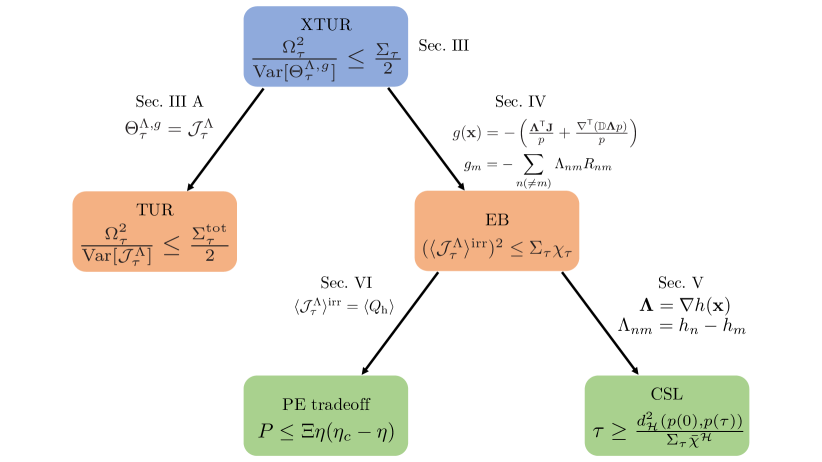
Figure 1: The hierarchical relationship among various thermodynamic tradeoff relations. Each box corresponds to an inequality, and each arrow illustrates the hierarchical connection between the inequalities it joins, along with the associated information specifying the conditions for deducing lower-level bounds.

II Notations and the main results

In this section, we present the key thermodynamic inequalities and their hierarchical relationship applicable to both Langevin and Markov jump systems. To facilitate this exploration, we begin by introducing the notations utilized throughout the paper.

II.1 Notations for Langevin systems

We consider an $N$-dimensional system whose state is described by the vector $\mathbf{x}=(x_{1},x_{2},\cdots,x_{N})^{\textsf{T}}$. Given a drift force $\mathbf{A}=(A_{1},A_{2},\cdots,A_{N})^{\textsf{T}}$ and a Gaussian white noise $\boldsymbol{\xi}=(\xi_{1},\xi_{2},\cdots,\xi_{N})^{\textsf{T}}$, the Langevin equation can be written as

$$\dot{\mathbf{x}}(t)=\mathbf{A}(\mathbf{x},\omega t)+\mathbb{B}(\mathbf{x},\omega t)\bullet\boldsymbol{\xi}(t)\;,$$ (1)

where $\omega$ is a parameter controlling the speed of the protocol, $\bullet$ denotes the Itô product, the noise satisfies $\langle\xi_{i}(t)\rangle=0$ and $\langle\xi_{i}(t)\xi_{j}(t^{\prime})\rangle=\delta_{ij}\delta(t-t^{\prime})$, and $\frac{1}{2}\mathbb{B}(\mathbf{x},\omega t)\,\mathbb{B}^{\textsf{T}}\!(\mathbf{x},\omega t)\equiv\mathbb{D}(\mathbf{x},\omega t)$ is a position-dependent diffusion matrix. The drift force can be divided into reversible and irreversible parts as $A_{i}=sf_{i}^{\text{rev}}(\mathbf{x},\omega t)+f_{i}^{\text{irr}}(\mathbf{x},\omega t)$, where $s$ is a parameter controlling the magnitude of the reversible drift. The two force components satisfy

$$f_{i}^{\text{rev}}(\boldsymbol{\epsilon}\mathbf{x},\omega t) =-\epsilon_{i}f_{i}^{\text{rev}}(\mathbf{x},\omega t)\;,$$

$$f_{i}^{\text{irr}}(\boldsymbol{\epsilon}\mathbf{x},\omega t) =\epsilon_{i}f_{i}^{\text{irr}}(\mathbf{x},\omega t)\;,$$ (2)

where we use the notation $\boldsymbol{\epsilon}\mathbf{x}\equiv(\epsilon_{1}x_{1},\epsilon_{2}x_{2},\cdots,\epsilon_{N}x_{N})$, with $\epsilon_{i}$ being the parity of variable $x_{i}$ under time reversal. Note that $s$ and $\omega$ are auxiliary variables that can be set to unity in the final step.

The equivalent Fokker-Planck equation is

$$\partial_{t}p(\mathbf{x},t;s,\omega)=-\nabla^{\textsf{T}}\left[\mathbf{J}^{\text{rev}}(\mathbf{x},t;s,\omega)+\mathbf{J}^{\text{irr}}(\mathbf{x},t;s,\omega)\right]\;,$$ (3)

where $\mathbf{J}^{\text{rev}}$ and $\mathbf{J}^{\text{irr}}$ are reversible and irreversible probability currents defined as

$$\mathbf{J}^{\text{rev}}=s\boldsymbol{f}^{\text{rev}}(\mathbf{x},\omega t)\,p(\mathbf{x},t;s,\omega)\;,$$

$$\mathbf{J}^{\text{irr}}=\left\{\boldsymbol{f}^{\text{irr}}(\mathbf{x},\omega t)-\left[\nabla^{\textsf{T}}\mathbb{D}(\mathbf{x},\omega t)\right]^{\textsf{T}}\right\}p(\mathbf{x},t;s,\omega)\;,$$ (4)

respectively, with the gradient $\nabla\equiv(\partial_{x_{1}},\partial_{x_{2}},\cdots,\partial_{x_{N}})^{\textsf{T}}$. The total probability current is then $\mathbf{J}\equiv\mathbf{J}^{\text{rev}}+\mathbf{J}^{\text{irr}}$. With these, the mean total EP can be written as

$$\Sigma_{\tau}^{\rm tot}=\int_{0}^{\tau}dt\int d\mathbf{x}\;\frac{{\mathbf{J}^{\rm irr}}^{\textsf{T}}\mathbb{D}^{-1}(\mathbf{x},\omega t)\mathbf{J}^{\rm irr}}{p(\mathbf{x},t;s,\omega)}.$$ (5)

For the brevity of notation, we shall henceforth omit the function arguments when there is no risk of confusion.

In this study, we consider both current-like and state-dependent observables, which take the forms

$$\mathcal{J}_{\tau}^{\Lambda}(\Gamma)\equiv\int_{0}^{\tau}dt\,\boldsymbol{\Lambda}^{\textsf{T}}\!(\mathbf{x}(t),\omega t;s)\circ\dot{\mathbf{x}}(t)\;,$$

$$\mathcal{K}_{\tau}^{g}(\Gamma)\equiv\int_{0}^{\tau}dt\,g(\mathbf{x}(t),\omega t;s)\;,$$ (6)

respectively. Here $\Gamma\equiv\{\mathbf{x}(t)\}$ denotes a stochastic trajectory, and $\circ$ stands for the Stratonovich product. In general, one can measure the composite observable $\Theta_{\tau}^{\Lambda,g}(\Gamma)$ involving these two:

$$\Theta_{\tau}^{\Lambda,g}(\Gamma)\equiv\mathcal{J}_{\tau}^{\Lambda}(\Gamma)+\mathcal{K}_{\tau}^{g}(\Gamma)\;.$$ (7)

Using the identity $\langle\boldsymbol{\Lambda}^{\textsf{T}}\circ\dot{\mathbf{x}}\rangle=\int d\mathbf{x}\,\boldsymbol{\Lambda}^{\textsf{T}}{\textbf{J}}$, the mean current-like observable can be separated into reversible and irreversible components as

$$\langle\mathcal{J}_{\tau}^{\Lambda}\rangle=\int_{0}^{\tau}dt\int d\mathbf{x}\,\boldsymbol{\Lambda}^{\textsf{T}}\mathbf{J}=\langle\mathcal{J}_{\tau}^{\Lambda}\rangle^{\rm rev}+\langle\mathcal{J}_{\tau}^{\Lambda}\rangle^{\rm irr}\;,$$ (8)

where $\langle\mathcal{J}_{\tau}^{\Lambda}\rangle^{\rm rev}\equiv\int_{0}^{\tau}dt\int d\mathbf{x}\,\boldsymbol{\Lambda}^{\textsf{T}}\mathbf{J}^{\rm rev}$ and $\langle\mathcal{J}_{\tau}^{\Lambda}\rangle^{\rm irr}\equiv\int_{0}^{\tau}dt\int d\mathbf{x}\,\boldsymbol{\Lambda}^{\textsf{T}}\mathbf{J}^{\rm irr}$.

II.2 Notations for Markov jump systems

Here we consider a continuous-time Markov jump process within a discrete state space $S$. The transition rate from state $m$ to $n$ at time $t$ is denoted by $R_{nm}(\omega t)$, where $\omega$ is the speed of the protocol. Then, the master equation of the system is given by

$$\dot{p}_{n}(t;\omega)=\sum_{m(\neq n)}j_{nm}(t;\omega)\;,$$ (9)

where $p_{n}(t;\omega)$ is the probability of finding the system in state $n\in S$ at time $t$, and $j_{nm}(t;\omega)=R_{nm}(\omega t)p_{m}(t;\omega)-R_{mn}(\omega t)p_{n}(t;\omega)$ is the net probability current from state $m$ to $n$. The mean total EP of this system is given by

$$\Sigma_{\tau}^{\rm tot}=\int_{0}^{\tau}dt\sum_{n>m}j_{nm}\ln\frac{R_{nm}p_{m}}{R_{mn}p_{n}}\;.$$ (10)

Moreover, we can define the mean pseudo-EP

$$\Sigma_{\tau}^{\text{ps}}\equiv\int_{0}^{\tau}dt\sum_{n\neq m}\frac{j_{nm}^{2}}{a_{nm}}\;,$$ (11)

where $a_{nm}=R_{nm}p_{m}+R_{mn}p_{n}$ is the dynamical activity between states $m$ and $n$. Using the log-mean inequality, one can prove

$$\Sigma^{\text{ps}}_{\tau}\leq\Sigma^{\text{tot}}_{\tau}\,.$$ (12)

Consider a trajectory of this Markov jump system, through which a total of $M$ jumps occur during the time interval $[0,\tau]$, with the $i$-th jump taking place at time $t_{i}$ for $i=1,2,\cdots,M$. For this trajectory, let us define $N_{nm}(t)$, the number of jumps from state $m$ to $n$ up to time $t$, and $\eta_{n}(t)\equiv\delta_{x(t),n}$, where $x(t)$ is the state of the system at time $t$. Note that these two observables satisfy $\langle\dot{N}_{nm}(t)\rangle=R_{nm}(\omega t)p_{m}(t;\omega)$ and $\langle\eta_{n}\rangle=p_{n}(t;\omega)$. Then, the current-like and the state-dependent observables can be written as

$$\mathcal{J}_{\tau}^{\Lambda}(\Gamma)\equiv\int_{0}^{\tau}dt\sum_{n\neq m}\Lambda_{nm}(\omega t)\dot{N}_{nm}(t)\;,~{}~{}~{}(\Lambda_{nm}=-\Lambda_{mn})$$

$$\mathcal{K}_{\tau}^{g}(\Gamma)\equiv\int_{0}^{\tau}dt\sum_{n}\eta_{n}(t)g_{n}(\omega t)\;,$$ (13)

respectively. Just as in the case of Langevin systems, one can measure the composite observable $\Theta_{\tau}^{\Lambda,g}(\Gamma)\equiv\mathcal{J}_{\tau}^{\Lambda}(\Gamma)+\mathcal{K}_{\tau}^{g}(\Gamma)$.

II.3 Main results

Our primary finding is a unified hierarchical framework integrating the four major thermodynamic inequalities (TUR, EB, CSL, and PE tradeoff) applicable to both Langevin and Markov jump systems. This hierarchy is depicted in Fig. 1. Each arrow in the figure, accompanied by its specifics, indicates how the lower-level inequality is deduced from the the one above it by constraining the associated observable. The reader is cautioned that, throughout this study, all expressions are given in units where the Boltzmann constant is equal to one.

At the apex of the hierarchy is the extended thermodynamic uncertainty relation (XTUR), which serves as the thermodynamic tradeoff relation for the most general class of the composite observable $\Theta_{\tau}^{\Lambda,g}(\Gamma)$. It is formulated as

$$\frac{\Omega_{\tau}^{2}}{\text{Var}[\Theta_{\tau}^{\Lambda,g}]}\leq\frac{\Sigma_{\tau}}{2}\;,$$ (14)

where $\Sigma_{\tau}$ can be either $\Sigma_{\tau}^{\rm tot}$ or $\Sigma_{\tau}^{\rm ps}$, and $\Omega_{\tau}$ is defined as

$$\Omega_{\tau}\equiv\hat{O}_{\tau}\langle\Theta_{\tau}^{\Lambda,g}\rangle-\langle\mathcal{K}_{\tau}^{g}\rangle+\left\langle\Theta_{\tau}^{s\partial_{s}\Lambda,s\partial_{s}g}\right\rangle\;,$$ (15)

with the operator $\hat{O}_{t}\equiv t\partial_{t}-s\partial_{s}-\omega\partial_{\omega}$ for both Langevin and Markov jump systems. We note that the terms associated with $s\partial_{s}$ in Eq. (15) vanish for systems with only even-parity variables since $s=0$ there. A derivation of Eq. (14) is given in Sec. III.

We stress that the XTUR represents the most comprehensive version of the TUR in the following sense: it provides an upper bound on the precision of the general composite observable even when the system involves odd-parity variables (including both momentum-like and force-like [33] ones) and time-dependent protocols. In contrast, prior research has predominantly focused on TURs for only current-like observables. While a handful of studies have ventured into deriving TURs for composite observables [34, 9, 35], their outcomes are restricted to the steady state and even-parity variables.

Starting from the XTUR, two other tradeoff relations are derived by restricting the form of the state-dependent observable. First, the conventional TUR for only current-like observables is readily obtained by setting the state-dependent observable to zero ($g=0$) within the XTUR, i.e., $\Theta_{\tau}^{\Lambda,g}(\Gamma)=\mathcal{J}_{\tau}^{\Lambda}(\Gamma)$ as shown in Fig. 1 and Sec. III. Alternatively, by selecting a state-dependent observable satisfying

$$g(\mathbf{x}) =-\left[\frac{\boldsymbol{\Lambda}^{\textsf{T}}\mathbf{J}}{p}+\frac{\nabla^{\textsf{T}}(\mathbb{D}\boldsymbol{\Lambda}p)}{p}\right]$$ (Langevin), (16)

$$g_{m} =-\sum_{n\neq m}\Lambda_{nm}R_{nm}$$ (Markov jump), (17)

where $p=p(\mathbf{x},t;s,\omega)$ is the probability density function, then the XTUR reduces to the EB

$$(\langle\mathcal{J}_{\tau}^{\Lambda}\rangle^{\rm irr})^{2}\leq\Sigma_{\tau}\chi_{\tau}\;,$$ (18)

where $\chi_{\tau}=\int_{0}^{\tau}dt\int d\mathbf{x}\langle\boldsymbol{\Lambda}^{\textsf{T}}\mathbb{D}\boldsymbol{\Lambda}\rangle$ for Langevin systems and $\chi_{\tau}=\frac{1}{2}\int_{0}^{\tau}dt\sum_{n<m}\Lambda_{nm}^{2}a_{nm}$ for Markov jump systems. This clarifies the relationship between the TUR and the EB: they are two different manifestations of a common higher-level tradeoff relation, the XTUR.

It is worth noting that, compared to the TUR, the EB offers a more experimentally accessible approach for estimating EP [32]. This can be attributed to the following two reasons. First, the EB inequality can always be saturated for arbitrary nonequilibrium processes, whereas this is not generally true for the TUR, as we discuss in Sec. III. Thus, while the accurate EP estimation can be made in the EB framework, the same level of accuracy is not guaranteed for the TUR method. Second, the EB lacks any differential operators, which the TUR must incorporate in the presence of odd-parity variables or time-dependent protocols. Empirical measurements of derivatives are often challenging, if not practically unfeasible. Thus, when dealing with time-dependent protocols or odd-parity variables, the EB offers a more feasible experimental framework than the TUR for EP estimation.

Now, proceeding further down the hierarchy, the absence of differential operators in the EB facilitates connections with the two lower-level thermodynamic tradeoff relations. The first of these is the CSL. By focusing on the overdamped Langevin systems with $\boldsymbol{\Lambda}=\nabla h(\mathbf{x})$ or the Markov jump systems with $\Lambda_{nm}=h_{n}-h_{m}$, and taking the supremum of Eq. (18) over a function space $\mathcal{H}$ of $h$, we obtain the following CSL:

$$\tau\geq\frac{d_{\mathcal{H}}^{2}(p(0),p(\tau))}{\Sigma_{\tau}\bar{\chi}^{\mathcal{H}}}\;,$$ (19)

where $d_{\mathcal{H}}(p,q)$ is the integral probability metric (IPM), which is a measure of distance between two distributions $p$ and $q$, and $\bar{\chi}^{\mathcal{H}}$ is the time average of the supremum of $\chi_{\tau}$. See Sec. V for details. From Eq. (19), we can derive a broad range of CSLs reported in the literature, such as the original CSL for Markov jump systems, Eq. (77) [22], the CSL involving the Wasserstein distance, Eq. (73), and the tighter CSL, Eq. (80) [36].

Finally, the other lower-level corollary of the EB is the PE tradeoff relation. For the case of Langevin systems, Dechant and Sasa have demonstrated that the PE tradeoff can be deduced from the EB for both steady-state and cyclic heat engines [19]. Meanwhile, Pietzonka and Seifert derived the PE tradeoff from the TUR, but solely for steady-state heat engines [28]. As for cyclic heat engines, however, establishing a link between the PE tradeoff and the TUR appears to be unattainable, primarily due to the inclusion of differential operators in the TUR formulation. In Sec. VI, we show that the EB makes it possible to derive the PE tradeoff for Markov jump systems, encompassing both steady-state and cyclic heat engines.

III XTUR

In this section, we present a derivation of the XTUR, situated at the apex of the hierarchy, for both Langevin and Markov jump systems. Following that, we delve into the equality condition of the XTUR, showing that it is achievable for the general nonequilibrium processes. Finally, we discuss the connection between the XTUR and the TUR.

III.1 XTUR for Langevin systems

Adapting a previously developed method [11, 14], the XTUR is derived by applying the Cramér–Rao inequality in conjunction with the perturbed dynamics described by the following Fokker-Planck equation:

$$\partial_{t}p_{\theta}=-\nabla^{\textsf{T}}\left[\mathbf{J}_{\theta}^{\text{rev}}+(1+\theta)\mathbf{J}_{\theta}^{\text{irr}}\right]\;,$$ (20)

where $\mathbf{J}_{\theta}^{\text{rev}}$ and $\mathbf{J}_{\theta}^{\text{irr}}$ are given by

$$\mathbf{J}_{\theta}^{\text{rev}}=s\mathbf{f}^{\text{rev}}p_{\theta}\;,\,\quad\mathbf{J}_{\theta}^{\text{irr}}=\left(\mathbf{f}^{\text{irr}}-\left[\nabla^{\textsf{T}}\mathbb{D}\right]^{\textsf{T}}\right)p_{\theta}\,.$$ (21)

In other words, the evolution of $p_{\theta}$ is achieved by multiplying the perturbation factor $1+\theta$ solely to the irreversible component of Eq. (3). It is straightforward to check that the solution of Eq. (20) is related to that of Eq. (3) by $p_{\theta}(\mathbf{x},t;s,\omega)=p(\mathbf{x},t_{\theta};s_{\theta},\omega_{\theta})$, where $t_{\theta}\equiv(1+\theta)t$, $s_{\theta}\equiv s/(1+\theta)$, and $\omega_{\theta}\equiv\omega/(1+\theta)$. Note that this scaling perturbation amounts to changing the drift vector $\mathbf{A}$ to $\mathbf{A}_{\theta}$ in the original Langevin dynamics described by Eq. (1) as follows:

$$\dot{\mathbf{x}}=\mathbf{A}_{\theta}+\mathbb{B}\bullet\boldsymbol{\xi}\;,~{}~{}~{}{\rm where}~{}~{}\mathbf{A}_{\theta}\equiv\mathbf{A}+\theta\frac{\mathbf{J}_{\theta}^{\text{irr}}}{p_{\theta}}\;.$$ (22)

Within this perturbation scheme, the XTUR is derived by taking $\theta=0$ in the Cramér–Rao inequality

$$\frac{(\partial_{\theta}\langle\Theta_{\tau}^{\Lambda,g}\rangle_{\theta})^{2}}{\text{Var}_{\theta}[\Theta_{\tau}^{\Lambda,g}]}\leq\mathcal{I}(\theta)\;,$$ (23)

where $\langle\cdots\rangle_{\theta}$ denotes the average over trajectories of the perturbed dynamics, and $\mathcal{I}(\theta)\equiv\langle-\partial_{\theta}^{2}\ln\mathcal{P}_{\theta}(\Gamma)\rangle_{\theta}$ represents the Fisher information associated with the path probability $\mathcal{P}_{\theta}(\Gamma)$ of the perturbed dynamics.

Evaluating the Fisher information at $\theta=0$ leads to

$$\mathcal{I}(0)=\frac{1}{2}\left(\Sigma^{\text{tot}}_{\tau}+\mathcal{B}\right)\;,$$ (24)

where the term $\mathcal{B}$ is determined by the dependence of the initial distribution on $s$ and $\omega$ (for details, see Appendix A.1). Opting for an initial distribution dependent on $s$ or $\omega$ yields a positive $\mathcal{B}$ [14]. In contrast, choosing an initial distribution independent of $s$ and $\omega$ leads to $\mathcal{B}=0$. There are some cases where a positive $\mathcal{B}$ leads to a tighter inequality (for a detailed explanation, see Appendix B); however, the case of $\mathcal{B}=0$ is more accessible to empirical measurement. Moreover, as discussed in Sec. IV, $\mathcal{B}=0$ allows us to derive the EB from the XTUR. Henceforth in this study, we adopt an initial distribution independent of $s$ and $\omega$, and thus, $\mathcal{B}=0$.

Evaluation of $\partial_{\theta}\langle\Theta_{\tau}^{\Lambda,g}\rangle_{\theta}\big{|}_{\theta=0}$ requires the calculations of both $\partial_{\theta}\langle\mathcal{J}_{\tau}^{\Lambda}\rangle_{\theta}\big{|}_{\theta=0}$ and $\partial_{\theta}\langle\mathcal{K}_{\tau}^{g}\rangle_{\theta}\big{|}_{\theta=0}$, which are given by

$$\partial_{\theta}\langle\mathcal{J}_{\tau}^{\Lambda}\rangle_{\theta}\big{|}_{\theta=0} =\hat{O}_{\tau}\langle\mathcal{J}_{\tau}^{\Lambda}\rangle+\int_{0}^{\tau}dt~{}\langle(s\partial_{s}\boldsymbol{\Lambda}^{\textsf{T}})\circ\dot{\textbf{x}}\rangle\;,$$

$$\partial_{\theta}\langle\mathcal{K}_{\tau}^{g}\rangle_{\theta}\big{|}_{\theta=0} =\hat{O}_{\tau}\langle\mathcal{K}_{\tau}^{g}\rangle-\langle\mathcal{K}_{\tau}^{g}\rangle+\int_{0}^{\tau}dt~{}\langle s\partial_{s}g\rangle\;.$$ (25)

Detailed derivations are presented in Appendix A.2. Adding these two equations results in

$$\partial_{\theta}\langle\Theta_{\tau}^{\Lambda,g}\rangle_{\theta}\big{|}_{\theta=0}=\hat{O}_{\tau}\langle\Theta_{\tau}^{\Lambda,g}\rangle-\langle\mathcal{K}_{\tau}^{g}\rangle+\left\langle\Theta_{\tau}^{s\partial_{s}\Lambda,s\partial_{s}g}\right\rangle,$$ (26)

where $\Theta_{\tau}^{s\partial_{s}\Lambda,s\partial_{s}g}=\int_{0}^{\tau}dt\,[(s\partial_{s}\boldsymbol{\Lambda}^{\textsf{T}})\circ\dot{\textbf{x}}+s\partial_{s}g]$. The right-hand side of Eq. (26) is none other than $\Omega_{\tau}$ written in Eq. (15). Substituting Eq. (24) with $\mathcal{B}=0$ and Eq. (26) into Eq. (23), we finally obtain the XTUR (14).

We now turn to the issue of when the XTUR inequality saturates. Given that the XTUR is derived from the Cramér–Rao inequality, its equality condition corresponds directly to that of the Cramér–Rao inequality. As shown in Eq. (18) of Ref. [11], the equality condition is

$$\Theta_{\tau}^{\Lambda,g}(\Gamma)-\langle\Theta_{\tau}^{\Lambda,g}\rangle_{\theta}=k(\theta)\partial_{\theta}\ln\mathcal{P}_{\theta}(\Gamma)\;,$$ (27)

where $k(\theta)$ is an arbitrary factor. For $\theta=0$, as detailed in Appendix A.3, this condition reduces to

$$\int_{0}^{\tau}dt\left\{{\mathbf{C}}_{1}^{\textsf{T}}\circ\dot{\mathbf{x}}(t)+{C}_{2}\right\}-\int_{0}^{\tau}dt\int d\mathbf{x}\,{C}_{3}=0$$ (28)

where ${\mathbf{C}}_{1}$, ${C}_{2}$, and ${C}_{3}$ are defined as

$${\mathbf{C}}_{1} \equiv\boldsymbol{\Lambda}-\frac{k(0)}{2}\frac{\mathbb{D}^{-1}\mathbf{J}^{\text{irr}}}{p}~{},$$

$${C}_{2} \equiv g+\frac{k(0)}{2}\left(\frac{{\mathbf{J}^{\text{irr}}}^{\mathsf{T}}\mathbb{D}^{-1}\mathbf{J}}{p^{2}}+\frac{\nabla^{\textsf{T}}\mathbf{J}^{\text{irr}}}{p}\right),$$

$${C}_{3} \equiv\boldsymbol{\Lambda}^{\textsf{T}}\mathbf{J}+gp~{}.$$ (29)

Since Eq. (28) must hold for all trajectories, the equality condition is satisfied only when $\textbf{C}_{1}={C}_{2}={C}_{3}=0$. The condition for $\mathbf{\Lambda}$ and $g$ to achieve $\textbf{C}_{1}=0$ and ${C}_{2}=0$ are

$$\boldsymbol{\Lambda}^{\rm eq} =\frac{k(0)}{2}\frac{\mathbb{D}^{-1}{\mathbf{J}}^{\text{irr}}}{p}~{},$$

$$g^{\rm eq} =-\frac{k(0)}{2}\left[\frac{{\mathbf{J}^{\text{irr}}}^{\textsf{T}}\mathbb{D}^{-1}{\mathbf{J}}}{p^{2}}+\frac{\nabla^{\textsf{T}}{\mathbf{J}}^{\text{irr}}}{p}\right]\;.$$ (30)

Interestingly, these $\boldsymbol{\Lambda}^{\rm eq}$ and $g^{\rm eq}$ also make $\int d{\textbf{x}}\,C_{3}$ vanish. Thus, Eq. (III.1) is the equality condition of the XTUR. It is worth noting that the equality condition cannot be met in the conventional TUR only with current-like observables (i.e., $g=0$), as $g^{\rm eq}$ is generally nonzero.

Finally, we discuss the connection between the XTUR and the previously discovered TURs. First, for overdamped systems without odd-parity variables, we can set $s=0$. For these systems, if we consider only current-like observables, then $g=0$. In this case, the XTUR is reduced to the Koyuk–Seifert TUR [12]

$$\frac{[(\tau\partial_{\tau}-\omega\partial_{\omega})\langle\mathcal{J}_{\tau}^{\Lambda}\rangle]^{2}}{\text{Var}[\mathcal{J}_{\tau}^{\Lambda}]}\leq\frac{\Sigma^{\text{tot}}_{\tau}}{2}\;,$$ (31)

which holds for overdamped processes driven by any time-dependent protocol. Alternatively, if we set $g=-\boldsymbol{\Lambda}^{\textsf{T}}{\mathbf{J}}/p$ for overdamped processes, the XTUR in the steady state becomes the relative TUR (RTUR) proposed by Dechant and Sasa [34], which is given by

$$\frac{\langle\mathcal{J}_{\tau}^{\Lambda}\rangle_{\text{ss}}^{2}}{\text{Var}_{\text{ss}}(\mathcal{J}_{\tau}^{\Lambda}+\mathcal{K}_{\tau}^{g})}\leq\frac{\Sigma^{\text{tot}}_{\tau}}{2}\;.$$ (32)

The XTUR can also be simplified to the TURs for underdamped Langevin dynamics. For the $N$-dimensional underdamped dynamics with position $\mathbf{x}=(x_{1},\cdots,x_{N})^{\textsf{T}}$ and momentum $\mathbf{p}=(p_{1},\cdots,p_{N})^{\textsf{T}}$, Eq. (1) can be rewritten as

$$\dot{x}_{i}=s\frac{p_{i}}{m_{i}}\;,$$

$$\dot{p_{i}}=sf_{i}^{\text{rev}}(\mathbf{x},\mathbf{p},\omega t)+f_{i}^{\text{irr}}(\mathbf{x},\mathbf{p},\omega t)-\frac{\gamma_{i}}{m_{i}}p_{i}+\xi_{i}\;,$$ (33)

where $m_{i}$, $\gamma_{i}$, and $\xi_{i}$ are the mass, the friction coefficient, and the Gaussian white noise corresponding to component $i$, respectively, with $\langle\xi_{i}(t)\xi_{j}(t^{\prime})\rangle=2\gamma_{i}T_{i}\delta_{ij}\delta(t-t^{\prime})$. We note that, in the underdamped dynamics, the diffusion matrix $\mathbb{D}$ is singular; however, one can directly apply our approach by simply replacing $\mathbb{D}^{-1}$ with the Moore–Penrose pseudoinverse. For the current-like observable defined as

$$\mathcal{J}_{\tau}^{\Lambda}(\Gamma)=\int_{0}^{\tau}dt\,\boldsymbol{\Lambda}(\mathbf{x},\mathbf{p},\omega t)\circ\dot{\mathbf{x}}\;,$$ (34)

it is straightforward to show that the XTUR reduces to the underdamped TUR

$$\frac{\Omega_{\tau}^{2}}{\text{Var}[\mathcal{J}_{\tau}^{\Lambda}]}\leq\frac{\Sigma^{\text{tot}}_{\tau}}{2}\;,$$ (35)

where $\Omega_{\tau}=\hat{O}_{\tau}\langle\mathcal{J}_{\tau}^{\Lambda}\rangle$. While this expression is analogous to the result of Ref. [14], there are a couple of notable differences. First, the term $\mathcal{B}$, dependent on the initial distribution, is absent due to our choice of an initial distribution independent of $s$ and $\omega$, as discussed earlier in this section. Second, while $\Omega_{\tau}$ in Ref. [14] involves a partial derivative with respect to the spatial rescaling parameter, no such term can be found in Eq. (35). This stems from the rescaling by $s$ of the inertia term $p_{i}/m_{i}$ in Eq. (III.1), which was not considered in Ref. [14].

III.2 XTUR for Markov jump systems

The method for deriving the XTUR presented above can also be adapted to Markov jump processes. For this purpose, we consider a perturbed Markov jump dynamics characterized by a modified transition rate $R_{nm}^{\theta}(\omega t)$, with its corresponding master equation expressed as

$$\dot{p}_{n}^{\theta}(t;\omega)=\sum_{m(\neq n)}j_{nm}^{\theta}(t;\omega)\,,$$ (36)

where $j_{nm}^{\theta}(t;\omega)=R_{nm}^{\theta}(\omega t)p_{m}^{\theta}(t;\omega)-R_{mn}^{\theta}(\omega t)p_{n}^{\theta}(t;\omega)$. Motivated by the approaches of Refs. [9, 29], we set the perturbed transition rate as $R_{nm}^{\theta}=R_{nm}e^{\theta K_{nm}^{\theta}}$ for $n\neq m$ and $R^{\theta}_{nn}=-\sum_{m(\neq n)}R^{\theta}_{mn}$ with respect to the original rate $R_{nm}$, where

$$K_{nm}^{\theta}(t;\omega)\equiv\frac{R_{nm}p_{m}^{\theta}-R_{mn}p_{n}^{\theta}}{R_{nm}p_{m}^{\theta}+R_{mn}p_{n}^{\theta}}\;.$$ (37)

Using the antisymmetry $K_{nm}^{\theta}=-K_{mn}^{\theta}$, we can show

$$R_{nm}p_{m}^{\theta}K_{nm}^{\theta}-R_{mn}p_{n}^{\theta}K_{mn}^{\theta}=R_{nm}p_{m}^{\theta}-R_{mn}p_{n}^{\theta}.$$ (38)

Then, for small $\theta$, Eq. (36) can be expanded as

$$\dot{p}_{n}^{\theta}= (1+\theta)\sum_{m(\neq n)}\left[R_{nm}(\omega t)p_{m}^{\theta}(t;\omega)-R_{mn}(\omega t)p_{n}^{\theta}(t;\omega)\right]$$

$$+O(\theta^{2})~{}.$$ (39)

One can readily check that the solution of this equation is given by $p_{n}^{\theta}(t;\omega)=p_{n}(t_{\theta};\omega_{\theta})+O(\theta^{2})$, where $p_{n}$ is the probability distribution of the original dynamics.

Similar to the approach of the previous section, in order to evaluate the Cramér–Rao inequality (23) at $\theta=0$, it is necessary to compute the Fisher information, $\partial_{\theta}\langle\mathcal{J}_{\tau}^{\Lambda}\rangle_{\theta}\big{|}_{\theta=0}$, and $\partial_{\theta}\langle\mathcal{K}_{\tau}^{g}\rangle_{\theta}\big{|}_{\theta=0}$. First, choosing the $\theta$-independent initial distribution, the Fisher information at $\theta=0$ is given by

$$\mathcal{I}(0)=\frac{1}{2}\Sigma_{\tau}^{\text{ps}}\leq\frac{1}{2}\Sigma_{\tau}^{\text{tot}}\;,$$ (40)

whose detailed derivation is presented in Appendix A.4. Note that the inequality originates from Eq. (12). Next, the mean current-like observable in the perturbed dynamics is obtained as

$$\langle\mathcal{J}_{\tau}^{\Lambda}\rangle_{\theta} =\int_{0}^{\tau}dt\sum_{n\neq m}\Lambda_{nm}(\omega t)p^{\theta}_{m}(t;\omega)R^{\theta}_{nm}(t;\omega)$$

$$=\int_{0}^{\tau}dt\sum_{n<m}\Lambda_{nm}(\omega t)j^{\theta}_{nm}(t;\omega)\;.$$ (41)

By expanding the probability current as $j_{nm}^{\theta}(t;\omega)=(1+\theta)j_{nm}(t_{\theta},\omega_{\theta})+O(\theta^{2})$, where $j_{nm}$ is the probability current of the original dynamics, we have

$$\langle\mathcal{J}_{\tau}^{\Lambda}\rangle_{\theta} =\int_{0}^{\tau_{\theta}}dt\sum_{n<m}\ \Lambda_{nm}\left(\omega_{\theta}t\right)j_{nm}\left(t;\omega_{\theta}\right)+O(\theta^{2})$$

$$=\langle\mathcal{J}_{\tau_{\theta}}^{\Lambda}\rangle|_{\omega=\omega_{\theta}}+O(\theta^{2})\;.$$ (42)

Therefore, we finally arrive at

$$\partial_{\theta}\langle\mathcal{J}_{\tau}^{\Lambda}\rangle_{\theta}\big{|}_{\theta=0}=\hat{O}_{\tau}\langle\mathcal{J}_{\tau}^{\Lambda}\rangle\;.$$ (43)

Similarly, we can prove that

$$\langle\mathcal{K}_{\tau}^{g}\rangle_{\theta} =\int_{0}^{\tau}dt\sum_{m}g_{m}(\omega t)p^{\theta}_{m}(t;\omega)$$

$$=\frac{1}{1+\theta}\int_{0}^{\tau_{\theta}}dt\sum_{m}\ g_{m}(\omega_{\theta}t)p_{m}\left(t;\omega_{\theta}\right)+O(\theta^{2})$$

$$=\left.\frac{1}{1+\theta}\langle\mathcal{K}_{\tau_{\theta}}^{g}\rangle\right|_{\omega=\omega_{\theta}}+O(\theta^{2})\;,$$ (44)

which leads to

$$\partial_{\theta}\langle\mathcal{K}_{\tau}^{g}\rangle_{\theta}\big{|}_{\theta=0}=(\hat{O}_{\tau}-1)\langle\mathcal{K}_{\tau}^{g}\rangle\;.$$ (45)

Plugging Eqs. (40), (43), and (45) into the Cramér–Rao inequality (23) yields the XTUR (14). Note that the terms associated with the operator $s\partial_{s}$ in the XTUR for Markov jump processes should vanish due to the lack of odd-parity variables.

The equality condition of the XTUR with $\Sigma_{\tau}=\Sigma_{\tau}^{\mathrm{ps}}$ for Markov jump systems is also identical to that of the Cramér–Rao inequality (27). From Eq. (II.2), the left-hand side of Eq. (27) at $\theta=0$ can be written as

$$\Theta_{\tau}^{\Lambda,g} (\Gamma)-\langle\Theta_{\tau}^{\Lambda,g}\rangle=\int_{0}^{\tau}dt\left(\sum_{n\neq m}\Lambda_{nm}\dot{N}_{nm}+\sum_{n}\eta_{n}g_{n}\right)$$

$$-\int_{0}^{\tau}dt\left(\sum_{n\neq m}\Lambda_{mn}p_{n}R_{mn}+\sum_{n}p_{n}g_{n}\right)\,.$$ (46)

By using the expression for the path probability (A.4), the right-hand side of Eq. (27) at $\theta=0$ can be evaluated as

$$\partial_{\theta}\ln\mathcal{P}_{\theta}(\Gamma)\big{|}_{\theta=0}$$

$$=-\int_{0}^{\tau}dt\sum_{n\neq m}\eta_{n}R_{mn}K_{mn}^{\theta=0}+\int_{0}^{\tau}dt\sum_{n\neq m}K_{nm}^{\theta=0}\dot{N}_{nm}\;.$$ (47)

Therefore, the equality condition can be rewritten as

$$0 =\int_{0}^{\tau}dt\sum_{n\neq m}\dot{N}_{nm}\left\{\Lambda_{nm}-k(0)K_{nm}^{\theta=0}\right\}$$

$$+\int_{0}^{\tau}dt\sum_{n}\eta_{n}\left\{g_{n}+k(0)\sum_{m(\neq n)}R_{mn}K_{mn}^{\theta=0}\right\}$$

$$-\int_{0}^{\tau}dt\sum_{n}p_{n}\left(\sum_{m(\neq n)}\Lambda_{mn}R_{mn}+g_{n}\right)\;.$$ (48)

Given that Eq. (III.2) holds for all trajectories, its every integrand must be identically zero. This condition is met when the observables satisfy $\Lambda_{nm}=\Lambda_{nm}^{\mathrm{eq}}$ and $g_{n}=g_{n}^{\mathrm{eq}}$, where

$$\Lambda_{nm}^{\rm eq}\equiv k(0)K_{nm}^{\theta=0},~{}~{}~{}g_{n}^{\rm eq}\equiv-k(0)\sum_{m(\neq n)}R_{mn}K_{mn}^{\theta=0}.$$ (49)

This is not attainable when all observables are current-like. Additionally, the condition ensures the saturation of the XTUR only when $\Sigma_{\tau}=\Sigma_{\tau}^{\rm ps}$. For the XTUR with $\Sigma_{\tau}=\Sigma_{\tau}^{\rm tot}$ to be saturated, the equality $\Sigma_{\tau}^{\rm ps}=\Sigma_{\tau}^{\rm tot}$ must hold, which is in general not fulfilled by $\Lambda_{nm}^{\rm eq}$ and $g_{n}^{\rm eq}$.

IV EB from XTUR

In this section, we show that the EB is derived from the XTUR by choosing a specific type of observables for both Langevin and Markov jump systems.

IV.1 Langevin systems

Converting the Stratonovich product to the Itô product according to Eq. (107), we can decompose the current-like observable $\mathcal{J}_{\tau}^{\Lambda}$ into two components:

$$\mathcal{J}_{\tau}^{\Lambda}(\Gamma) =\int_{0}^{\tau}dt\,\boldsymbol{\Lambda}^{\textsf{T}}\circ\dot{\mathbf{x}}$$

$$=\int_{0}^{\tau}dt\,\boldsymbol{\Lambda}^{\textsf{T}}\bullet\dot{\mathbf{x}}+\int_{0}^{\tau}dt\,\text{tr}\,[\mathbb{D}\nabla\boldsymbol{\Lambda}^{\textsf{T}}]\;.$$ (50)

If we set $g$ in the state-dependent observable as

$$g^{\rm EB}(\mathbf{x},\omega t;s)=-\boldsymbol{\Lambda}^{\textsf{T}}(s\mathbf{f}^{\text{rev}}+\mathbf{f}^{\text{irr}})-\text{tr}\,[\mathbb{D}\nabla\boldsymbol{\Lambda}^{\textsf{T}}]\;,$$ (51)

then the composite observable becomes

$$\Theta_{\tau}^{\Lambda,g^{\rm EB}}(\Gamma)=\int_{0}^{\tau}dt\,\boldsymbol{\Lambda}^{\textsf{T}}\mathbb{B}(\mathbf{x},\omega t)\bullet\boldsymbol{\xi}(t)\;.$$ (52)

Using the Gaussian statistics of $\boldsymbol{\xi}(t)$, it is straightforward to show that $\langle\Theta_{\tau}^{\Lambda,g^{\rm EB}}\rangle=0$ and

$$\text{Var}(\Theta_{\tau}^{\Lambda,g^{\rm EB}})=\left\langle\left(\Theta_{\tau}^{\Lambda,g^{\rm EB}}\right)^{2}\right\rangle=2\int_{0}^{\tau}dt\,\langle\boldsymbol{\Lambda}^{\textsf{T}}\mathbb{D}\boldsymbol{\Lambda}\rangle\;.$$ (53)

In addition, using $\langle\Theta_{\tau}^{\Lambda,g^{\rm EB}}\rangle=0$ in Eq. (7), we have

$$\langle\mathcal{K}_{\tau}^{g^{\rm EB}}\rangle=-\langle\mathcal{J}_{\tau}^{\Lambda}\rangle.$$ (54)

Meanwhile, using the relations $s\mathbf{f}^{\text{rev}}+\mathbf{f}^{\text{irr}}=\mathbf{J}/p+(\nabla^{\textsf{T}}\mathbb{D}p)^{\textsf{T}}/p$ and

$$\nabla^{\textsf{T}}[\mathbb{D}\boldsymbol{\mathbf{V}}p]=\text{tr}\,[\mathbb{D}\nabla\mathbf{V}^{\textsf{T}}]\,p+\mathbf{V}^{\textsf{T}}(\nabla^{\textsf{T}}\mathbb{D}p)^{\textsf{T}}$$ (55)

that holds for any $N$-dimensional vector $\mathbf{V}$, from Eq. (51) we obtain

$$s\partial_{s}g^{\rm EB}=-\frac{(s\partial_{s}\boldsymbol{\Lambda}^{\textsf{T}})\mathbf{J}}{p}-\frac{1}{p}\nabla^{\textsf{T}}[\mathbb{D}(s\partial_{s}\boldsymbol{\Lambda})p]-\frac{\boldsymbol{\Lambda}^{\textsf{T}}\mathbf{J}^{\rm rev}}{p}.$$ (56)

Then, utilizing Eq. (56), the third term in Eq. (15) is evaluated as

$$\left\langle\Theta_{\tau}^{s\partial_{s}\Lambda,s\partial_{s}g^{\rm EB}}\right\rangle =\int_{0}^{\tau}dt\,\int d\mathbf{x}\,(s\partial_{s}\boldsymbol{\Lambda}^{\textsf{T}}\mathbf{J}+s\partial_{s}g^{\rm EB}p)$$

$$=-\int_{0}^{\tau}dt\,\int d\mathbf{x}\,\boldsymbol{\Lambda}^{\textsf{T}}\mathbf{J}^{\text{rev}}\;.$$ (57)

Combining Eqs. (54) and (IV.1), $\Omega_{\tau}$ in Eq. (15) becomes

$$\Omega_{\tau} =\int_{0}^{\tau}dt\int d\mathbf{x}\,\boldsymbol{\Lambda}^{\textsf{T}}\mathbf{J}-\int_{0}^{\tau}dt\int d\mathbf{x}\,\boldsymbol{\Lambda}^{\textsf{T}}\mathbf{J}^{\text{rev}}$$

$$=\int_{0}^{\tau}dt\int d\mathbf{x}\,\boldsymbol{\Lambda}^{\textsf{T}}\mathbf{J}^{\text{irr}}=\langle\mathcal{J}_{\tau}^{\Lambda}\rangle^{\text{irr}}\;.$$ (58)

Finally, putting Eqs. (53) and (IV.1) into the XTUR yields the EB (18). Note that Eq. (51) for $g^{\rm EB}$ can be transformed into the form shown in Eq. (16) using Eq. (55).

IV.2 Markov jump systems

Noting that the EB for Markov jump systems has not previously been established, we first prove it without relying on any other thermodynamic inequalities. Starting with the definition of the current-like observable for Markov jump systems, shown in Eq. (II.2), we derive the EB as follows:

$$\langle\mathcal{J}_{\tau}^{\Lambda}\rangle^{2} =\left(\int_{0}^{\tau}dt\sum_{n<m}\Lambda_{nm}j_{nm}\right)^{2}$$

$$\leq\frac{1}{2}\int_{0}^{\tau}dt\sum_{n<m}\Lambda_{nm}^{2}a_{nm}\times 2\int_{0}^{\tau}dt\sum_{n<m}\frac{j_{nm}^{2}}{a_{nm}}$$

$$=\chi_{\tau}\Sigma^{\text{ps}}_{\tau}\leq\chi_{\tau}\Sigma^{\text{tot}}_{\tau}\;,$$ (59)

where $\chi_{\tau}\equiv\frac{1}{2}\int_{0}^{\tau}dt\sum_{n<m}\Lambda_{nm}^{2}a_{nm}$. For the inequalities in the second and the third lines, the Cauchy–Schwarz inequality and Eq. (12) are used, respectively.

Now, we show that Eq. (IV.2) can be derived from the XTUR for Markov jump systems. Towards this aim, we set the function $g$ as

$$g_{m}^{\rm EB}=-\sum_{n(\neq m)}\Lambda_{nm}R_{nm}\;.$$ (60)

Then, the composite observable $\Theta_{\tau}^{\Lambda,g^{\rm EB}}=\mathcal{J}_{\tau}^{\Lambda}+\mathcal{K}_{\tau}^{g^{\rm EB}}$ takes the form

$$\Theta_{\tau}^{\Lambda,g^{\rm EB}}=\int_{0}^{\tau}dt\sum_{n\neq m}\Lambda_{nm}(\omega t)\,[\dot{N}_{nm}(t)-\eta_{m}(t)R_{nm}(\omega t)]\;.$$ (61)

Using the relations $\langle\dot{N}_{nm}\rangle=R_{nm}p_{m}$ and $\langle\eta_{n}\rangle=p_{n}$, we obtain $\langle\Theta_{\tau}^{\Lambda,g^{\rm EB}}\rangle=0$, which implies $\langle\mathcal{J}_{\tau}^{\Lambda}\rangle=-\langle\mathcal{K}_{\tau}^{g^{\rm EB}}\rangle$. Moreover, we can derive

$$\text{Var}(\Theta_{\tau}^{\Lambda,g^{\rm EB}})=\int_{0}^{\tau}dt\sum_{n\neq m}\Lambda_{nm}^{2}R_{nm}p_{m}=2\chi_{\tau}\,,$$ (62)

as detailed in Appendix A.5. Combining these results with the XTUR (14) for $\Sigma_{\tau}=\Sigma_{\tau}^{\mathrm{ps}}$, we arrive at the EB as given in Eq. (IV.2).

V CSL from EB

In this section, we show how the CSL can be derived from the EB. To achieve this, we first introduce the integral probability metric (IPM) [37, 38, 39], which quantifies the statistical difference between two probability distributions. Then the CSL is derived by applying the IPM within the EB framework.

V.1 Integral Probability Metric (IPM)

The IPM is a metric quantifying the distance between two probability distributions. For any pair of distributions $p$ and $q$, the IPM is defined as

$$d_{\mathcal{H}}(p,q)=\sup_{h\in\mathcal{H}}\left|\langle h\rangle_{p}-\langle h\rangle_{q}\right|\;,$$ (63)

where $\mathcal{H}$ represents a set of functions with some specific properties, and $\langle h\rangle_{p}$ and $\langle h\rangle_{q}$ are the expectation values of the function $h$ with respect to $p$ and $q$, respectively.

There are some notable examples of the IPM. First, when $\mathcal{H}$ is a set of functions bounded within the range $[-1,1]$, the IPM is equal to twice the total variation distance [39], i.e., $d_{\mathcal{H}}(p,q)=2d_{\text{TV}}(p,q)$, where

$$d_{\text{TV}}(p,q) \equiv\frac{1}{2}\sum_{x\in\Omega}|p(x)-q(x)|$$

$$=\frac{1}{2}\sup_{h\in[-1,1]}|\langle h\rangle_{p}-\langle h\rangle_{q}|\;.$$ (64)

Second, we consider the case where $\mathcal{H}$ is the set of Lipschitz-$1$ functions, defined as $\text{Lip}_{1}\equiv\{h|d(x,y)\geq|h(x)-h(y)|,\,\forall x,y\}$, where $d(x,y)$ represents the distance between $x$ and $y$. In this case, due to the Kantorovich–Rubinstein duality [40, 41], the IPM coincides with the Wasserstein-$1$ distance

$$d_{\text{Lip}_{1}}(p,q)=\mathcal{W}_{1}(p,q)\;,$$ (65)

which is widely used in the context of the optimal transport problem [40, 41, 42]. For the continuous random variables, the Wasserstein-$1$ distance is defined as

$$\mathcal{W}_{1}(p,q)\equiv\inf_{\pi(\mathbf{x},\mathbf{y})\in\Phi(p,q)}\int d\mathbf{x}\,d\mathbf{y}\,d(\mathbf{x},\mathbf{y})\,\pi(\mathbf{x},\mathbf{y})\;,$$ (66)

where $\Phi(p,q)$ stands for the set of all joint probability distributions $\pi(\mathbf{x},\mathbf{y})$ whose marginals are given by $\int d\mathbf{y}\,\pi=p$ and $\int d\mathbf{x}\,\pi=q$. For Langevin systems, $d(\mathbf{x},\mathbf{y})$ is typically taken to be the Euclidean distance $|\mathbf{x}-\mathbf{y}|$. Meanwhile, for discrete random variables, the definition changes to

$$\mathcal{W}_{1}(p,q)\equiv\inf_{\pi_{nm}\in\Phi(p,q)}\sum_{n,m}d_{nm}\pi_{nm}\;,$$ (67)

where $\Phi(p,q)$ is the set of all joint probability distributions $\pi_{nm}$ which satisfies $\sum_{m}\pi_{nm}=p_{n}$ and $\sum_{n}\pi_{nm}=q_{m}$. For Markov jump systems, the distance $d_{nm}$ is typically set to be the length of the shortest path between states $n$ and $m$ in the graph representation of possible transitions. See Appendix A.6 for more details about the Wasserstein-1 distance on graphs.

V.2 CSL for Langevin systems

Employing the IPM introduced above, the CSL (19) can be deduced from the EB (18) by appropriately limiting the associated observable to a specific form. Since the CSL has been studied for systems without odd-parity variables, here we focus on the overdamped Langevin systems.

We start by defining $\mathcal{D}$ as the set of functions that are continuous and almost everywhere differentiable in $\mathbb{R}^{N}$. Let $\mathcal{H}$ be a subset of $\mathcal{D}$. Then, for any function $h\in\mathcal{H}$, $\nabla h(\mathbf{x})$ exists everywhere except for a measure-zero subset $V_{h}\subset\mathbb{R}^{N}$. With this in mind, we choose the current-like observable satisfying

$$\boldsymbol{\Lambda}=\begin{cases}\nabla h(\mathbf{x}),~{}\ &\text{if $\mathbf{x}\in\mathbb{R}^{N}\backslash V_{h}$,}\\ \boldsymbol{\Lambda}_{0}(\mathbf{x}),~{}\ &\text{if $\mathbf{x}\in V_{h}$,}\end{cases}$$ (68)

where $\boldsymbol{\Lambda}_{0}$ is an arbitrary vector field. Then the mean value of the current-like observable is given by

$$\langle\mathcal{J}_{\tau}^{\Lambda}\rangle =\int_{0}^{\tau}dt\int_{\mathbb{R}^{N}\backslash V_{h}}d\mathbf{x}\,(\nabla^{\textsf{T}}h)\,\mathbf{J}+\int_{0}^{\tau}dt\int_{V_{h}}d\mathbf{x}\,\boldsymbol{\Lambda}_{0}^{\textsf{T}}\mathbf{J}$$

$$=\int_{0}^{\tau}dt\int_{\mathbb{R}^{N}}d\mathbf{x}\,h(\mathbf{x})\,\partial_{t}p(\mathbf{x},t)$$

$$=\langle h\rangle_{p(\tau)}-\langle h\rangle_{p(0)}\;,$$ (69)

where $\langle h\rangle_{p(t)}\equiv\int d\mathbf{x}\,h(\mathbf{x})p(\mathbf{x},t)$. Integration by parts and $\partial_{t}p=-\nabla\cdot\mathbf{J}$ have been used to obtain the second equality, along with the fact that $V_{h}$ is a measure-zero set and does not contribute to the integral. Using this result in Eq. (18) and taking the supremum over $h\in\mathcal{H}$, the EB transforms into

$$d^{2}_{\mathcal{H}}(p(0),p(\tau))\leq\Sigma^{\text{tot}}_{\tau}\chi^{\mathcal{H}}_{\tau}\;,$$ (70)

where $\chi^{\mathcal{H}}_{\tau}\equiv\sup_{h\in\mathcal{H}}\int_{0}^{\tau}dt\int_{\mathbb{R}^{N}\backslash V_{h}}d\mathbf{x}\,p\nabla h^{T}\mathbb{D}\nabla h$ is a constant that depends on the choice of $\mathcal{H}$. Since $\chi^{\mathcal{H}}_{\tau}$ is a time-extensive quantity, we can define its time average $\bar{\chi}^{\mathcal{H}}\equiv\chi^{\mathcal{H}}_{\tau}/\tau$. Then, Eq. (70) can be rewritten in the standard CSL form as

$$\tau\geq\frac{d_{\mathcal{H}}^{2}(p(0),p(\tau))}{\Sigma_{\tau}^{\rm tot}\bar{\chi}^{\mathcal{H}}}\;.$$ (71)

By choosing a proper $\mathcal{H}$, various CSLs can be derived from this inequality. For example, let us take $\mathcal{H}=\text{Lip}_{1}\subset\mathcal{D}$. Then, as stated in Eq. (65), $d_{\text{Lip}_{1}}$ corresponds to the Wasserstein-$1$ distance. As for $\chi_{\tau}^{\text{Lip}_{1}}$, since every $h\in\text{Lip}_{1}$ satisfies $|\nabla h(\mathbf{x})|\leq 1$, we obtain

$$\chi_{\tau}^{\text{Lip}_{1}} =\sup_{h\in\text{Lip}_{1}}\int_{0}^{\tau}dt\int_{\mathbb{R}^{N}\backslash V_{h}}d\mathbf{x}\,p\nabla h^{T}\mathbb{D}\nabla h$$

$$\leq\int_{0}^{\tau}dt\int d\mathbf{x}\,\rho[\mathbb{D}(\mathbf{x},\omega t)]\,p(\mathbf{x},t)=\int_{0}^{\tau}dt\,\langle\rho[\mathbb{D}]\rangle\;,$$ (72)

where $\rho(\mathbb{A})$ is the largest absolute eigenvalue of the matrix $\mathbb{A}$. Then, the CSL can be rewritten as

$$\tau\geq\frac{\mathcal{W}_{1}^{2}(p(0),p(\tau))}{\Sigma_{\tau}^{\rm tot}\overline{\langle\rho(\mathbb{D})\rangle}}\;,$$ (73)

where $\overline{\langle\rho(\mathbb{D})\rangle}\equiv\frac{1}{\tau}\int_{0}^{\tau}dt\,\langle\rho(\mathbb{D})\rangle$. If the diffusion matrix is uniform in $\mathbf{x}$ and $t$, we can replace $\overline{\langle\rho(\mathbb{D})\rangle}$ with $\rho(\mathbb{D})$. Or, if the diffusion matrix is an identity matrix multiplied by time-dependent temperature $T(\mathbf{x},t)$, then $\overline{\langle\rho(\mathbb{D})\rangle}=\frac{1}{\tau}\int_{0}^{\tau}dt\,\langle T(\mathbf{x},t)\rangle$, where $\langle T(\mathbf{x},t)\rangle=\int d\mathbf{x}\,T(\mathbf{x},t)\,p(\mathbf{x},t)$.

It is worth highlighting that the CSL presented in Eq. (73), a novel contribution of this study, is generally applicable to systems featuring a diffusion matrix which is neither diagonal nor uniform in $\mathbf{x}$ and $t$. This is distinct from the previous CSLs for overdamped Langevin systems, which focused on systems immersed a single heat bath at fixed temperature [43, 25, 44, 27]. Additionally, we emphasize our use of the Wasserstein-$1$ distance instead of the Wasserstein-$2$ distance employed in previous works [43, 25, 44, 27]. The difference is rooted in the fact that the Wasserstein-$1$ distance belongs to the category of the IPM, while the Wasserstein-$2$ distance does not.

V.3 CSL for Markov jump systems

The CSL for Markov jump systems can also be derived from the EB when the associated current-like observable meets the gradient condition $\Lambda_{nm}=h_{n}-h_{m}\equiv\nabla h_{nm}$. Then, its ensemble average satisfies

$$\langle\mathcal{J}_{\tau}^{\nabla h}\rangle =\int_{0}^{\tau}dt\sum_{n>m}(h_{n}-h_{m})j_{nm}=\int_{0}^{\tau}dt\sum_{n\neq m}h_{n}j_{nm}$$

$$=\int_{0}^{\tau}dt\sum_{n}h_{n}\dot{p}_{n}(t)=\langle h\rangle_{p(\tau)}-\langle h\rangle_{p(0)}\;,$$ (74)

where $\dot{p}_{n}(t)=\sum_{m(\neq n)}j_{nm}$ has been used for the third equality, and $\langle h\rangle_{p(t)}\equiv\sum_{n}h_{n}p_{n}\!(t)$. Using this relation, the EB (18) for $\Sigma_{\tau}=\Sigma_{\tau}^{\mathrm{ps}}$ reduces to

$$d^{2}_{\mathcal{H}}(p(0),p(\tau))\leq\Sigma^{\text{ps}}_{\tau}\chi_{\tau}^{\mathcal{H}}\;,$$ (75)

where $\chi_{\tau}^{\mathcal{H}}\equiv\frac{1}{2}\sup_{h\in\mathcal{H}}\int_{0}^{\tau}dt\sum_{n<m}(h_{n}-h_{m})^{2}a_{nm}$. Since $\Sigma^{\text{ps}}_{\tau}\leq\Sigma^{\text{tot}}_{\tau}$, once again we obtain Eq. (71), proving that the CSL for Markov jump systems can also be formulated in the same form.

For concreteness, let us examine the case of $\mathcal{H}=\mathcal{H}_{1}\equiv\{h_{n}|h_{n}\in[-1,1]\}$. Then, as discussed above Eq. (V.1), $d_{\mathcal{H}}$ is related to the total variation distance. Besides, since $|h_{n}-h_{m}|\leq 2$ for all $n$ and $m$, we obtain

$$\chi_{\tau}^{\mathcal{H}_{1}}\leq 2\int_{0}^{\tau}dt\sum_{n<m}a_{nm}=2\mathcal{A}_{\tau}\;,$$ (76)

where $\mathcal{A}_{\tau}$ is the dynamical activity. Denoting its time average as $\bar{\mathcal{A}}\equiv\mathcal{A}_{\tau}/\tau$, Eq. (75) implies

$$\tau\geq\frac{d_{\text{TV}}^{2}(p(0),p(\tau))}{\Sigma_{\tau}^{\rm tot}\bar{\mathcal{A}}/2}\;,$$ (77)

which reproduces the original CSL derived in Ref. [22].

Another CSL, recently discovered [36] and proven to be tighter than Eq. (77), can also be derived from Eq. (75). Let $f(x)$ be the inverse function of $f^{-1}(x)=x\tanh x$. Then, Eqs. (75) and (76) lead to the following inequalities:

$$\frac{d_{\mathcal{H}_{1}}^{2}}{2\mathcal{A}_{\tau}}\leq\frac{d_{\mathcal{H}_{1}}^{2}}{\chi_{\tau}^{\mathcal{H}_{1}}}\leq\Sigma^{\text{ps}}_{\tau}\leq\frac{(\Sigma_{\tau}^{\text{tot}})^{2}}{2\mathcal{A}_{\tau}}f\left(\frac{\Sigma_{\tau}^{\text{tot}}}{2\mathcal{A}_{\tau}}\right)^{-2}\;.$$ (78)

The final inequality can be derived using Eq. (10) of Ref. [29]. These yield $f(\Sigma_{\tau}^{\text{tot}}/2\mathcal{A_{\tau}})\leq\Sigma_{\tau}^{\text{tot}}/d_{\mathcal{H}_{1}}$, which in turn implies

$$\frac{\Sigma_{\tau}^{\text{tot}}}{2\mathcal{A}_{\tau}}\leq f^{-1}\left(\frac{\Sigma_{\tau}^{\text{tot}}}{d_{\mathcal{H}_{1}}}\right)=\frac{\Sigma_{\tau}^{\text{tot}}}{d_{\mathcal{H}_{1}}}\tanh\left(\frac{\Sigma_{\tau}^{\text{tot}}}{d_{\mathcal{H}_{1}}}\right)\;.$$ (79)

Finally, using $d_{\mathcal{H}_{1}}=2d_{\text{TV}}$, we arrive at

$$\tau\geq\frac{d_{\text{TV}}}{\bar{\mathcal{A}}\tanh\left(\frac{\Sigma_{\tau}^{\text{tot}}}{2d_{\text{TV}}}\right)}\;,$$ (80)

reproducing the tighter CSL proven in Ref. [36].

Yet another application of Eq. (75) is the CSL for Markov jump systems in terms of the Wasserstein distance. To show this, we select $\mathcal{H}=\textrm{Lip}_{1}$, which equates $d_{\mathcal{H}}$ to the Wasserstein-1 distance, as stated in Eq. (65). For Markov jump systems, $\textrm{Lip}_{1}$ can be expressed as

$$\text{Lip}_{1}=\left\{h_{n}|1\geq|h_{n}-h_{m}|\,\,\text{for all }(n,m)\in E\right\}\;,$$ (81)

where $E$ denotes the set of all state pairs joined by allowed transitions. A detailed proof is provided in Appendix A.6. Using the above property of $\text{Lip}_{1}$, it is straightforward to obtain

$$\chi^{\text{Lip}_{1}}_{\tau}\leq\frac{1}{2}\int_{0}^{\tau}dt\sum_{n<m}a_{nm}=\frac{1}{2}\mathcal{A}_{\tau}\;.$$ (82)

Combining these results with Eq. (75), we derive

$$\tau\geq\frac{\mathcal{W}_{1}^{2}(p(0),p(\tau))}{\Sigma_{\tau}^{\rm tot}\bar{\mathcal{A}}/2}\;.$$ (83)

As was done for the case of the original CSL discussed above, a tighter version of the above CSL, namely

$$\tau\geq\frac{\mathcal{W}_{1}}{\bar{\mathcal{A}}\tanh\left(\frac{\Sigma_{\tau}^{\rm tot}}{2\mathcal{W}_{1}}\right)}\;,$$ (84)

can be derived using inequalities similar to Eq. (78). This result is equivalent to Eq. (57) of Ref. [26] and Eq. (129) of Ref. [27]. As discussed in [27], Eq. (84) is generally saturable for any graphs, while Eq. (80) can be saturated only for fully-connected graphs.

These derivations provide clear evidence that Eq. (75), essentially the EB for a specific class of current-like observables, is a foundational CSL from which follows a broad range of CSLs reported in the literature.

VI PE tradeoff from EB

Consider a heat engine that operates between hot and cold heat reservoirs characterized by the temperatures $T_{\rm h}$ and $T_{\rm c}$ $(T_{\rm h}>T_{\rm c})$, respectively. Let $Q_{\rm h}$ denote the heat absorbed from the hot reservoir, $Q_{\rm c}$ the heat dissipated into the cold reservoir, and $W$ the work extracted from the engine. Then, the PE tradeoff relation can be expressed as [21]

$$P\leq\Xi\eta(\eta_{\rm C}-\eta)\,,$$ (85)

where $P$ is the power of the engine, $\Xi$ a system-dependent constant, $\eta\equiv\langle W\rangle/\langle Q_{\rm h}\rangle$ the efficiency of the engine, and $\eta_{\rm C}=1-T_{\rm c}/T_{\rm h}$ the Carnot efficiency. This relation dictates that it is impossible to achieve $\eta_{\rm C}$ and finite power simultaneously, even though an irreversible process can sometimes achieve $\eta_{\rm C}$ [45, 46]. This tradeoff relation has been proven for both steady-state and cyclic engines in Langevin systems using the EB [19]. It has also been derived using the TUR [28], but solely for the steady-state engines and not for the cyclic engines. In this section, we establish the PE tradeoff for both steady-state and cyclic engines in Markov jump systems using the EB.

To achieve this goal, we consider a heat engine consisting of discrete $N$ states in contact with two heat reservoirs, each characterized by a temperature denoted as $T_{k}$ ($k\in\{{\rm h},{\rm c}\}$). The energy associated with each state is represented as $E_{n}(t)$ ($n\in\{1,2,\ldots,N\}$). The transition rate from state $n$ to state $m$ under the influence of heat reservoir $k$ is expressed as $R_{mn}^{k}(\omega t)$, which satisfies the local detailed balance condition: $R_{mn}^{k}e^{-E_{n}/T_{k}}=R_{nm}^{k}e^{-E_{m}/T_{k}}$. The master equation governing this system is given by

$$\dot{p}_{n}=\sum_{m(\neq n),k}j_{nm}^{k}\;,$$ (86)

where $j_{nm}^{k}=R_{nm}^{k}p_{m}-R_{mn}^{k}p_{n}$. We are interested in the current-like observables expressed as

$$\mathcal{J}_{\tau}^{\Delta E,k}=\int_{0}^{\tau}dt\sum_{n\neq m}\Delta E_{nm}\dot{N}_{nm}^{k}\,,$$ (87)

where $\Delta E_{nm}=E_{n}-E_{m}$, and $N_{nm}^{k}$ is the number of jumps from state $m$ to $n$ under the influence of reservoir $k$ until time $t$. Then, we can readily identify $\mathcal{J}_{\tau}^{\Delta E,{\rm h}}=Q_{\rm h}$ and $\mathcal{J}_{\tau}^{\Delta E,{\rm c}}=-Q_{\rm c}$. Choosing $Q_{\rm h}$ as the observable appearing in the EB, we obtain

$$\langle Q_{\rm h}\rangle^{2}\leq\tau\bar{\chi}^{\rm h}\Sigma_{\tau}^{\rm tot},$$ (88)

where $\bar{\chi}^{\rm h}=\frac{1}{2\tau}\int_{0}^{\tau}dt\sum_{n\neq m}\Delta E_{nm}^{2}a_{nm}^{\rm h}$ with $a_{nm}^{\rm h}=R_{nm}^{\rm h}p_{n}+R_{mn}^{\rm h}p_{m}$. When the engine is in the periodic state, we choose $\tau$ to be the period of a cycle. Then, since the energy of the system does not change after each cycle, we have $\Sigma_{\tau}^{\rm tot}=\langle Q_{\rm c}\rangle/T_{\rm c}-\langle Q_{\rm h}\rangle/T_{\rm h}=(\eta_{\rm C}-\eta)\langle Q_{\rm h}\rangle/T_{\rm c}$. Using this expression in Eq. (88) and multiplying both sides of the inequality by $\eta=\langle W\rangle/\langle Q_{\rm h}\rangle$, we finally derive

$$P\leq\frac{\bar{\chi}^{\rm h}}{T_{\rm c}}\eta(\eta_{\rm C}-\eta),$$ (89)

where $P=\langle W\rangle/\tau$. It is straightforward to adapt this proof to the same inequality for steady-state engines. We stress that Eq. (89) is an equivalent of the PE tradeoff relation shown in Eq. (85), but extended to both cyclic and steady-state engines built using Markov jump systems.

For completeness, we note that the PE tradeoff for Langevin systems can also be derived from the EB by choosing the heat from the hot reservoir as the observable of interest, as previously shown in Ref. [19]. Thus, the EB provides a reliable starting point for deducing the PE tradeoff for a broad range of engines. In contrast, to our knowledge, it seems impossible to derive the PE tradeoff for cyclic engines starting from the TUR.

VII Examples

In this section, we present concrete illustrations of two tradeoff relations derived in this study: the EB for Markov jumps systems and the CSL for the Langevin systems subject to an inhomogeneous temperature field.

VII.1 EB for two-level batteries

As an example of the EB for Markov jump systems, we consider a charging-discharging process utilizing a two-level system, as depicted in Fig. 2(a). The energy of each state is denoted by $E_{i}(t)$ for $i=1,2$. During the charging process with duration $\tau_{\rm c}$, $E_{1}(t)>E_{2}(t)$ is maintained so that the particle tends to escape state $1$ to charge state $2$. Conversely, in the discharging process with duration $\tau_{\rm d}$, $E_{1}(t)<E_{2}(t)$ is maintained so that the particle is discharged from state $2$, releasing the energy $E_{2}(t)-E_{1}(t)$ via each transition. For simplicity, we assume that $E_{2}(t)$ is kept constant at $\Delta$, while $E_{1}(t)=2\Delta$ during the charging process and $E_{1}(t)=0$ during the discharging process. Then, keeping the local detailed balance, the transition rates are given by

$$R_{21}(t) =\frac{\mu(t)}{1+e^{-\beta[E_{1}(t)-\Delta]}}\,,$$

$$R_{12}(t) =\frac{\mu(t)e^{-\beta[E_{1}(t)-\Delta]}}{1+e^{-\beta[E_{1}(t)-\Delta]}}\;,$$ (90)

where $\beta$ is the inverse temperature, and $\mu(t)$ controls the overall rate of transitions. Suppose we are concerned with quantifying the speed of the charging-discharging process. This can be quantified by the current-like observable $\mathcal{J}_{\tau}^{\Lambda}$ satisfying $\Lambda_{nm}(t)=\text{sgn}[E_{m}(t)-E_{n}(t)]$, which counts the excess number of charging and discharging transitions compared to the number of opposite transitions hindering the process.

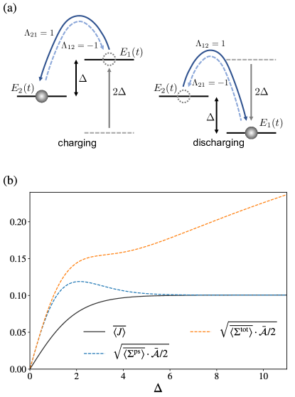
Figure 2: (a) Schematic illustration of the charging-discharging process. During the charging phase, the energy level of state 1 is increased, charging the battery by prompting the particle to jump to state 2. In contrast, during the discharging phase, the energy level of state 1 is decreased below that of state 2, resulting in battery discharge. In each phase, $\Delta$ represents the energy gap between the two states. (b) Verification of the EB (91) for the charging-discharging process. The black solid line depicts the mean charging-discharging speed. The dashed curves represent the EBs set by the mean EP and the mean pseudo-EP.

Since $\Lambda_{nm}^{2}=1$ within this setup, $\chi_{\tau}$ in the EB (IV.2) reduces to the dynamical activity $\mathcal{A}_{\tau}$. Then, the EB is rewritten as $\langle\mathcal{J}_{\tau}\rangle\leq\sqrt{\mathcal{A}_{\tau}\Sigma_{\tau}/2}$. In the periodic state, we can define the mean charging-discharging speed as $\overline{\langle J\rangle}\equiv\langle\mathcal{J}_{\tau_{\rm c}+\tau_{\rm d}}^{\Lambda}\rangle/(\tau_{\rm c}+\tau_{\rm d})$, the mean EP as $\overline{\langle\Sigma^{\text{tot}}\rangle}\equiv\langle\Sigma_{\tau_{\rm c}+\tau_{\rm d}}^{\text{tot}}\rangle/(\tau_{\rm c}+\tau_{\rm d})$, the mean pseudo-EP as $\overline{\langle\Sigma^{\text{ps}}\rangle}\equiv\langle\Sigma_{\tau_{\rm c}+\tau_{\rm d}}^{\text{ps}}\rangle/(\tau_{\rm c}+\tau_{\rm d})$, and the mean dynamical activity as $\bar{\mathcal{A}}\equiv\mathcal{A}_{\tau_{\rm c}+\tau_{\rm d}}/(\tau_{\rm c}+\tau_{\rm d})$. Using these definitions, we obtain the upper bounds on the charging-discharging speed

$$\overline{\langle J\rangle}\leq\sqrt{\overline{\langle\Sigma^{\text{ps}}\rangle}\bar{\mathcal{A}}/2}\leq\sqrt{\overline{\langle\Sigma^{\text{tot}}\rangle}\bar{\mathcal{A}}/2}\;.$$ (91)

The behaviors of $\overline{\langle J\rangle}$, $\sqrt{\overline{\langle\Sigma^{\text{ps}}\rangle}\bar{\mathcal{A}}/2}$, and $\sqrt{\overline{\langle\Sigma^{\text{tot}}\rangle}\bar{\mathcal{A}}/2}$ as functions of the energy gap $\Delta$ are shown in Fig. 2(b) for $\tau_{\rm c}=\tau_{\rm d}=10$, $\mu(t)=1$, and $\beta=1$. Besides their consistency with the inequalities of Eq. (91), two points merit attention. First, the difference between the two upper bounds is negligible for small $\Delta$, which corresponds to the near-equilibrium regime. Second, the charging-discharging speed saturates to the tighter upper bound set by the pseudo-EP for large $\Delta$. This behavior stems from the equality condition of the tighter upper bound, which is given by

$$\Lambda_{nm}^{\rm eq}=\frac{p_{m}R_{nm}-p_{n}R_{mn}}{p_{m}R_{nm}+p_{n}R_{mn}}\;.$$ (92)

In the limit of large $\Delta$, since the transitions become almost totally irreversible, this quantity becomes either $1$ or $-1$ for every transition until the occupation probability of the higher energy level reaches zero. For transitions occurring afterwards, the quantity may have different values, but such transitions negligibly contribute to the physical quantities. Hence, the observable with $\Lambda_{nm}(t)=\Lambda_{nm}^{\rm eq}$ is practically equal to our chosen observable with $\Lambda_{nm}(t)=\text{sgn}[E_{m}(t)-E_{n}(t)]$, thus ensuring the saturation of the tighter bound. In contrast, the weaker bound by the total EP cannot be saturated in this regime, as the discrepancy between the EP and the pseudo-EP increases as the system moves farther away from equilibrium.

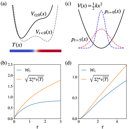
Figure 3: (a) Illustration of the tilted double-well potential and the nonuniform temperature field. The dashed and the solid lines represent the potential for $t<0$ and $t\geq 0$, respectively. The colormap below the potential indicates the temperature field, which is colder (hotter) on the left (right). (b) Verification of the CSL (73) for the process depicted in (a). (c) Illustration of the probability distribution (dashed curves) broadening within a harmonic potential (solid curve) as temperature increases with time. (d) Verification of the CSL (73) for the process depicted in (c).

VII.2 CSL in Langevin systems subjected to inhomogeneous temperature field

To illustrate the CSL in a nonuniform temperature field, we consider a one-dimensional Brownian particle trapped in either a single-well or a double-well potential [36]. Its equation of motion is given by

$$\gamma\dot{x}=-\frac{\partial V(x,t)}{\partial x}+\sqrt{2\gamma T(x,t)}\bullet\xi(t)\;,$$ (93)

where $\xi(t)$ is a Gaussian white noise satisfying $\langle\xi(t)\rangle=0$ and $\langle\xi(t)\xi(t^{\prime})\rangle=\delta(t-t^{\prime})$. We note that the spatial inhomogeneity in the noise amplitude stems only from the temperature field $T(x,t)$ and not from the constant friction coefficient $\gamma$, in which case the Itô description of the multiplicative noise is indeed appropriate in the overdamped limit, as discussed in Ref. [47].

We verify the CSL for two different processes of the system. The first example concerns the relaxation of the Brownian particle when the potential $V(x)$ and the temperature field $T(x)$ are abruptly changed. More specifically, we consider the potential

$$V(x) =V_{\text{DW}}(x)+\Theta_{\text{tilt}}\frac{x}{x_{m}}\,,$$ (94)

where $V_{\text{DW}}(x)=E_{b}[\left(x/x_{m}\right)^{4}-2\left(x/x_{m}\right)^{2}]$ is a double-well potential, and $\Theta_{\text{tilt}}$ controls the magnitude of the linear tilting potential. This potential has widely been used to investigate the finite-time Landauer principle [48, 36] governing the entropic cost of erasing one bit of information. Meanwhile, the temperature field is given by

$$T(x) =T_{0}\left(1+\delta\tanh\frac{x}{x_{T}}\right)\,,$$ (95)

where $\delta$ and $x_{T}$ control the magnitude and the length scale of temperature change across the system, respectively. For $t<0$, both $\Theta_{\textrm{tilt}}$ and $\delta$ are set to zero, letting the particle equilibrate in the bare double-well potential $V_{\text{DW}}(x)$ to the uniform temperature field $T(x)=T_{0}=1$. Then, at $t=0$, we set $\Theta_{\rm tilt}=2$ and $\delta=0.5$, switching on the tilting potential and the nonuniform temperature field, as illustrated in Fig. 3(a). This protocol amounts to erasing one bit of information encoded by the Brownian particle by tuning both the potential and the temperature field. Given the other parameters fixed at $\gamma=1$, $x_{m}=1$, $x_{T}=0.2$, and $E_{b}=1$, Fig. 3(b) verifies the CSL stated in Eq. (73), where $\overline{\langle T\rangle}\equiv\frac{1}{\tau}\int_{0}^{\tau}dt\langle T(x,t)\rangle$ plays the role of $\overline{\langle\rho(\mathbb{D})\rangle}$. Thus, Eq. (73) provides a way to study the finite-time Landauer principle involving the local heating as well as the potential manipulation.

The next example pertains to the Brownian particle confined in a harmonic potential $V(x)=\frac{1}{2}kx^{2}$ with the temperature of the heat bath changing in time as

$$T(t)=\begin{cases}T_{0}&\text{for $t<0$}\;,\\ T_{0}(1+t/\tau_{\rm T})&\text{for $t\geq 0$}\;.\end{cases}$$ (96)

This means that the particle distribution becomes broader as time goes by, as illustrated in Fig. 3(c). Choosing $k=1$ and $\tau_{\rm T}=1/4$, in Fig. 3(d) we demonstrate the validity of the CSL stated in Eq. (73).

VIII Conclusion

Through this study, we have unveiled the hierarchical connections among various thermodynamic tradeoff relations, encompassing the TUR, the EB, the CSL, and the PE tradeoff. This hierarchy commences with the XTUR, which deals with the most general types of observables. All the other tradeoff relations stem from the XTUR by imposing specific constraints upon the associated observable. When state-dependent observables are excluded, the XTUR simplifies to the TUR. On the other hand, choosing state-dependent observables as described in Eqs. (51) and (60) transforms the XTUR into the EB. Further down the hierarchy, focusing on the systems without odd-parity variables, the CSL and the PE tradeoff follow from the EB by employing the heat current and the IPM as the associated current-like observable, respectively.

This hierarchy offers a fundamental and comprehensive perspective on the landscape of significant thermodynamic inequalities that have emerged in the field of nonequilibrium thermodynamics over the past decade. In particular, the structure indicates that the TUR, the EB, the CSL, and the PE tradeoff can all be categorized under a single class of thermodynamic relations, which we might call the XTUR class. Hence, if future research uncovers another thermodynamic inequality, one critical task will be to ascertain whether this new relation falls within the XTUR class or deviates from it. The latter case would suggest that the inequality is truly new and may open up the avenue towards a hitherto unexplored realm of thermodynamics.

For the future research, it is highly desirable to extend our theory to open quantum systems [49, 50, 51, 52, 53, 54, 16, 17, 23, 18, 27]. Over the past decade, numerous thermodynamic tradeoff relations have also emerged in the quantum domain, such as the quantum TURs [16, 17, 18, 31] and the quantum speed limits [54, 23, 27, 31]. However, these relations have largely been investigated as independent properties. Therefore, a critical forthcoming task is to establish a unified hierarchical framework for these tradeoff relations governing open quantum systems. This will facilitate a deeper understanding of quantum thermodynamics and its applications.

Acknowledgments. — The authors thank Su-Chan Park for fruitful discussions. This research has been supported by the POSCO Science Fellowship of POSCO TJ Park Foundation (E.K. and Y.B.), KIAS Individual Grant No. PG064901 (J.S.L.), and an appointment to the JRG Program at the APCTP through the Science and Technology Promotion Fund and Lottery Fund of the Korean Government (J.-M.P.). This was also supported by the Korean Local Governments - Gyeongsangbuk-do Province and Pohang City (J.-M.P.).

Appendix A Detailed derivations

A.1 Fisher information in Langevin systems, Eq. (24)

When the system follows the modified Langevin dynamics governed by Eq. (22), its path probability satisfies [55]

$$\mathcal{P}_{\theta}[\Gamma]=\mathcal{N}p(0)\,e^{-\frac{1}{4}\int_{0}^{\tau}dt\,(\dot{\mathbf{x}}-\mathbf{A}_{\theta})^{\textsf{T}}\bullet\mathbb{D}^{-1}\bullet(\dot{\mathbf{x}}-\mathbf{A}_{\theta})},$$ (97)

where $\mathcal{N}$ is the normalization constant, and $p(0)\equiv p(\textbf{x},0;s,\omega)$ is the initial probability distribution. Then, we have

$$\partial^{2}_{\theta}\ln\mathcal{P}_{\theta}=\frac{1}{2}\int_{0}^{\tau}dt\,\partial^{2}_{\theta}\mathbf{A}_{\theta}^{\textsf{T}}\mathbb{D}^{-1}\bullet(\dot{\mathbf{x}}-\mathbf{A}_{\theta})$$

$$\,\,\,\,\,\,\,\,-\frac{1}{2}\int_{0}^{\tau}dt\,\partial_{\theta}\mathbf{A}_{\theta}^{\textsf{T}}\mathbb{D}^{-1}\partial_{\theta}\mathbf{A}_{\theta}+\frac{\partial_{\theta}^{2}p(0)}{p(0)}-\frac{\{\partial_{\theta}p(0)\}^{2}}{p(0)^{2}}.$$ (98)

Using $\partial_{\theta}\mathbf{A}_{\theta}\big{|}_{\theta=0}=\mathbf{J}^{\text{irr}}/p$ and $\langle\dot{\textbf{x}}-\textbf{A}_{\theta}\rangle_{\theta}=0$, the Fisher information at $\theta=0$ is obtained as

$$\mathcal{I}(0) =\langle-\partial^{2}_{\theta}\ln\mathcal{P}_{\theta}\rangle_{\theta=0}$$

$$=\frac{1}{2}\int_{0}^{\tau}dt\int d\mathbf{x}\,\frac{{\mathbf{J}^{\text{irr}}}^{\textsf{T}}\mathbb{D}^{-1}\mathbf{J}^{\text{irr}}}{p}$$

$$\qquad+\left\langle\left[(s\partial_{s}+\omega\partial_{\omega})\ln p(0)\right]^{2}\right\rangle=\frac{1}{2}\left(\Sigma^{\text{tot}}_{\tau}+\mathcal{B}\right)\;,$$ (99)

where $\mathcal{B}=2\langle\left[(s\partial_{s}+\omega\partial_{\omega})\ln p(0)\right]^{2}\rangle$. If we choose an initial distribution independent of $s$ and $\omega$, then $\mathcal{B}=0$.

A.2 Evaluation of $\partial_{\theta}\langle\mathcal{J}_{\tau}^{\Lambda}\rangle|_{\theta=0}$ and $\partial_{\theta}\langle\mathcal{K}_{\tau}^{g}\rangle|_{\theta=0}$, Eq. (III.1)

We begin by evaluating $\partial_{\theta}\langle\mathcal{J}_{\tau}^{\Lambda}\rangle|_{\theta=0}$. Through direct substitution, we can show that the total probability current $\mathbf{J}_{\theta}\equiv\mathbf{J}_{\theta}^{\rm rev}+(1+\theta)\mathbf{J}_{\theta}^{\rm irr}$ of the modified dynamics governed by Eq. (22) is related to the original current by $\mathbf{J}_{\theta}({\textbf{x}},t;s,\omega)=(1+\theta)\mathbf{J}({\textbf{x}},t_{\theta};s_{\theta},\omega_{\theta})$. Using this relation, the mean of $\mathcal{J}_{\tau}^{\Lambda}$ in the modified dynamics is obtained as

$$\langle\mathcal{J}_{\tau}^{\Lambda}\rangle_{\theta} =\int_{0}^{\tau}dt\int d\mathbf{x}\,\boldsymbol{\Lambda}^{\textsf{T}}({\textbf{x}},\omega t;s)\mathbf{J}_{\theta}({\textbf{x}},t;s,\omega)$$

$$=\int_{0}^{\tau}dt\int d\mathbf{x}\,(1+\theta)\boldsymbol{\Lambda}^{\textsf{T}}({\textbf{x}},\omega t;s)\mathbf{J}({\textbf{x}},t_{\theta};s_{\theta},\omega_{\theta})$$

$$=\int_{0}^{\tau_{\theta}}dt\int d\mathbf{x}\,\boldsymbol{\Lambda}^{\textsf{T}}\left({\textbf{x}},\omega_{\theta}t;s\right)\mathbf{J}({\textbf{x}},t;s_{\theta},\omega_{\theta})\;.$$ (100)

The Taylor expansion $\boldsymbol{\Lambda}(\mathbf{x},\omega_{\theta}t;s)=\boldsymbol{\Lambda}(\mathbf{x},\omega_{\theta}t;s_{\theta})+\theta s_{\theta}\partial_{s}\boldsymbol{\Lambda}(\mathbf{x},\omega_{\theta}t;s)|_{s=s_{\theta}}+O(\theta^{2})$ yields

$$\langle\mathcal{J}_{\tau}^{\Lambda}\rangle_{\theta} =\langle\mathcal{J}_{\tau_{\theta}}^{\Lambda}\rangle|_{s=s_{\theta},\omega=\omega_{\theta}}$$

$$+\theta\int_{0}^{\tau_{\theta}}dt\,s_{\theta}\partial_{s}\boldsymbol{\Lambda}^{\textsf{T}}|_{s=s_{\theta}}\mathbf{J}({\textbf{x}},t;s_{\theta},\omega_{\theta})+O(\theta^{2}).$$ (101)

Differentiating both sides of this equation with respect to $\theta$ and setting $\theta=0$, we arrive at

$$\partial_{\theta}\langle\mathcal{J}_{\tau}^{\Lambda}\rangle_{\theta}\big{|}_{\theta=0} =\hat{O}_{\tau}\langle\mathcal{J}_{\tau}^{\Lambda}\rangle+\int_{0}^{\tau}dt~{}\langle(s\partial_{s}\boldsymbol{\Lambda}^{\textsf{T}})\circ\dot{\textbf{x}}\rangle\,.$$ (102)

Now, we turn to the evaluation of $\partial_{\theta}\langle\mathcal{K}_{\tau}^{g}\rangle|_{\theta=0}$. The mean of $\mathcal{K}_{\tau}^{g}$ in the modified dynamics satisfies

$$\langle\mathcal{K}_{\tau}^{g}\rangle_{\theta} =\int_{0}^{\tau}dt\int d\mathbf{x}\,g(\mathbf{x},\omega t;s)p_{\theta}(\mathbf{x},t;s,\omega)$$

$$=\frac{1}{1+\theta}\int_{0}^{\tau_{\theta}}dt\int d\mathbf{x}\,g(\omega_{\theta}t;s)p(t;s_{\theta},\omega_{\theta})\,.$$ (103)

Proceeding with the Taylor expansion $g(\mathbf{x},\omega_{\theta}t;s)=g(\mathbf{x},\omega_{\theta}t;s_{\theta})+\theta s_{\theta}\partial_{s}g(\mathbf{x},\omega_{\theta}t;s)|_{s=s_{\theta}}+O(\theta^{2})$, we obtain

$$\langle\mathcal{K}_{\tau}^{g}\rangle_{\theta} =\frac{1}{1+\theta}\langle\mathcal{K}_{\tau_{\theta}}\rangle|_{s=s_{\theta},\omega=\omega_{\theta}}$$

$$+\theta\int_{0}^{\tau}dt\,s_{\theta}\partial_{s}g|_{s=s_{\theta}}p(t;s_{\theta},\omega_{\theta})+O(\theta^{2})\,.$$ (104)

Differentiating both sides with respect to $\theta$, we finally derive

$$\partial_{\theta}\langle\mathcal{K}_{\tau}^{g}\rangle_{\theta}\big{|}_{\theta=0} =\hat{O}_{\tau}\langle\mathcal{K}_{\tau}^{g}\rangle-\langle\mathcal{K}_{\tau}^{g}\rangle+\int_{0}^{\tau}dt~{}\langle s\partial_{s}g\rangle\;.$$ (105)

A.3 XTUR saturation for Langevin systems, Eq. (28)

From the definition of $\Theta_{\tau}^{\Lambda,g}$, the left-hand side of Eq. (27) at $\theta=0$ can be written as

$$\Theta_{\tau}^{\Lambda,g}(\Gamma)-\langle\Theta_{\tau}^{\Lambda,g}\rangle= \int_{0}^{\tau}dt\left(\boldsymbol{\Lambda}^{\textsf{T}}\circ\dot{{\textbf{x}}}+g\right)$$

$$-\int_{0}^{\tau}dt\int d{\textbf{x}}\left(\boldsymbol{\Lambda}^{\textsf{T}}{\textbf{J}}+gp\right)\,.$$ (106)

To compute the right-hand side of Eq. (27), we must use the conversion relationship between the Stratonovich and the Itô products

$$\mathbf{h}^{\textsf{T}}(\mathbf{x},t)\circ d\mathbf{x}=\mathbf{h}^{\textsf{T}}(\mathbf{x},t)\bullet d\mathbf{x}+\text{tr}[\mathbb{D}\nabla\mathbf{h}^{\textsf{T}}(\mathbf{x},t)]\,dt\;,$$ (107)

which holds for an arbitrary function $\mathbf{h}(\mathbf{x},t)$. Here, we have used the relation $d\mathbf{x}=\mathbf{A}dt+\mathbb{B}\bullet d\mathbf{W}$, where $\mathbf{W}$ stands for the Wiener process. To derive this formula, one starts from the definition of the Stratonovich product

$$h_{i}(\mathbf{x},t)\circ dx_{i}=\frac{1}{2}\left[h_{i}(\mathbf{x}+d\mathbf{x},t+dt)+h_{i}(\mathbf{x},t)\right]dx_{i}\;.$$ (108)

Keeping the terms up to the order of $dt$, the right-hand side can be expanded as

$$h_{i}(\mathbf{x},t)\circ dx_{i}=h_{i}(\mathbf{x},t)\bullet dx_{i}+\frac{1}{2}\sum_{j}\partial_{x_{j}}h_{i}(\mathbf{x},t)dx_{i}dx_{j}\;.$$ (109)

Using $dx_{i}dx_{j}=\sum_{k,l}\mathbb{B}_{ik}\mathbb{B}_{jl}dW_{k}dW_{l}+O(dt^{3/2})$ and the heuristic Itô rule $dW_{k}dW_{l}=\delta_{kl}dt$, this simplifies to

$$h_{i}(\mathbf{x},t)\circ dx_{i}=h_{i}(\mathbf{x},t)\bullet dx_{i}+\sum_{j}\mathbb{D}_{ij}\partial_{x_{j}}h_{i}(\mathbf{x},t)dt\;.$$ (110)

Summing this equation side by side over $i$, we derive the conversion formula shown in Eq. (107).

Using Eqs. (97),  (107), and (22), we can rewrite Eq. (27) at $\theta=0$ as

$$\partial_{\theta}\log\mathcal{P}_{\theta}(\Gamma)\big{|}_{\theta=0}$$

$$=\frac{1}{2}\int_{0}^{\tau}dt~{}\frac{{\mathbf{J}^{\text{irr}}}^{\textsf{T}}}{p}\mathbb{D}^{-1}\bullet(\dot{\mathbf{x}}-\mathbf{A})$$

$$=\frac{1}{2}\int_{0}^{\tau}dt~{}\frac{{\mathbf{J}^{\text{irr}}}^{\textsf{T}}}{p}\mathbb{D}^{-1}\circ\dot{\mathbf{x}}-\frac{1}{2}\int_{0}^{\tau}dt~{}\text{tr}\left[\mathbb{D}\nabla\left(\frac{{\mathbf{J}^{\text{irr}}}^{\textsf{T}}}{p}\mathbb{D}^{-1}\right)\right]$$

$$~{}~{}~{}-\frac{1}{2}\int_{0}^{\tau}dt\left[\frac{{\mathbf{J}^{\text{irr}}}^{\textsf{T}}\mathbb{D}^{-1}\{\mathbf{J}+(\nabla^{\textsf{T}}\mathbb{D}p)^{\textsf{T}})\}}{p^{2}}\right]\;.$$ (111)

Here we note that

$$\textrm{tr}\left[\mathbb{D}\nabla\left(\frac{{\mathbf{J}^{\text{irr}}}^{\textsf{T}}}{p}\mathbb{D}^{-1}\right)\right]=\mathbb{D}_{ij}\partial_{x_{j}}\!\left[\frac{J^{\text{irr}}_{k}(\mathbb{D}^{-1})_{ki}}{p}\right]$$

$$=\left[\partial_{x_{j}}(\mathbb{D}^{-1})_{ki}\right]\mathbb{D}_{ij}\frac{J^{\text{irr}}_{k}}{p}+\nabla^{\textsf{T}}\left(\frac{\mathbf{J}^{\text{irr}}}{p}\right)$$

$$=-\frac{{\mathbf{J}^{\text{irr}}}^{\textsf{T}}\mathbb{D}^{-1}}{p}(\nabla^{\textsf{T}}\mathbb{D})^{\textsf{T}}-\frac{\nabla p^{\textsf{T}}\mathbf{J}^{\text{irr}}}{p^{2}}+\frac{\nabla^{\textsf{T}}\mathbf{J}^{\text{irr}}}{p}$$

$$=-\frac{{\mathbf{J}^{\text{irr}}}^{\textsf{T}}\mathbb{D}^{-1}(\nabla^{\textsf{T}}\mathbb{D}p)^{\textsf{T}}}{p^{2}}+\frac{\nabla^{\textsf{T}}\mathbf{J}^{\text{irr}}}{p}\;.$$ (112)

For the third equality in Eq. (A.3), $\mathbb{D}_{ij}\partial_{x_{j}}(\mathbb{D}^{-1})_{ki}=-(\mathbb{D}^{-1})_{ki}\partial_{x_{j}}\mathbb{D}_{ij}$ has been used since $\partial_{x_{j}}[(\mathbb{D}^{-1})_{ki}\mathbb{D}_{ij}]=\partial_{x_{j}}\delta_{kj}=0$. By substituting the outcome of Eq. (A.3) into Eq. (A.3), we arrive at

$$\partial_{\theta}\log\mathcal{P}_{\theta}(\Gamma)\big{|}_{\theta=0}$$

$$=\frac{1}{2}\int_{0}^{\tau}dt\left(\frac{{\mathbf{J}^{\text{irr}}}^{\textsf{T}}}{p}\mathbb{D}^{-1}\circ\dot{\mathbf{x}}-\frac{{\mathbf{J}^{\text{irr}}}^{\textsf{T}}\mathbb{D}^{-1}\mathbf{J}}{p^{2}}-\frac{\nabla^{\textsf{T}}\mathbf{J}^{\text{irr}}}{p}\right)\;.$$ (113)

Finally, plugging Eqs. (A.3) and (A.3) into Eq. (27), we obtain the equality condition stated in Eq. (28).

A.4 Fisher information in Markov jump systems, Eq. (40)

When the system follows the modified Markov jump process satisfying Eq. (36), then its path probability is given by [56, 57]

$$\mathcal{P}[\Gamma] =p_{n_{0}}(0)\exp\bigg{[}\int_{0}^{\tau}dt\sum_{n}\eta_{n}(t)R_{nn}^{\theta}(\omega t)$$

$$~{}~{}~{}~{}~{}~{}~{}~{}~{}~{}~{}~{}~{}+\int_{0}^{\tau}dt\sum_{n\neq m}\ln R^{\theta}_{nm}(\omega t)\dot{N}_{nm}\bigg{]}\;,$$ (114)

where $p_{n_{0}}(0)$ represents the initial-state distribution, set to be independent of the perturbing parameters. Note that the first and the second terms in the exponent correspond to the sums of the staying and the transition probabilities, respectively. Then, the Fisher information satisfies

$$\mathcal{I}(\theta)=-\langle\partial^{2}_{\theta}\log\mathcal{P}[\Gamma]\rangle_{\theta}$$

$$=-\int_{0}^{\tau}dt\sum_{n}p^{\theta}_{n}\partial^{2}_{\theta}R^{\theta}_{nn}-\int_{0}^{\tau}dt\sum_{n\neq m}p^{\theta}_{m}R^{\theta}_{nm}\partial^{2}\ln R^{\theta}_{nm}$$

$$=\int_{0}^{\tau}dt\sum_{n\neq m}\left(p_{m}^{\theta}\partial^{2}_{\theta}R^{\theta}_{nm}-p^{\theta}_{m}R^{\theta}_{nm}\partial^{2}_{\theta}\ln R^{\theta}_{nm}\right)$$

$$=\int_{0}^{\tau}dt\sum_{n\neq m}p^{\theta}_{m}R^{\theta}_{nm}(\partial_{\theta}\ln R^{\theta}_{nm})^{2}\;.$$ (115)

Hence, the Fisher information at $\theta=0$ is obtained as

$$\mathcal{I}(0) =\int_{0}^{\tau}dt\sum_{n\neq m}p_{m}R_{nm}(K_{nm}^{\theta=0})^{2}$$

$$=\frac{1}{2}\int_{0}^{\tau}dt\sum_{n\neq m}a_{nm}(K_{nm}^{\theta=0})^{2}=\frac{1}{2}\Sigma_{\tau}^{\text{ps}}\;.$$ (116)

A.5 Variance of the current-like observable
in Markov jump processes, Eq. (62)

The number of jumps from state $m$ to state $n$ during an infinitesimal time interval $dt$, namely $\dot{N}_{nm}dt=N_{nm}(t+dt)-N_{nm}(t)$, can be factorized as $\eta_{m}(t)T_{nm}(t)dt$, where $T_{nm}(t)dt$ denotes the number of jump from state $m$ to state $n$ provided that the system is in the state $m$ at time $t$. Here, $T_{nm}(t)dt=1$ with probability $R_{nm}(t)dt$ and $T_{nm}dt=0$ with probability $1-R_{nm}(t)dt$, which implies $\langle T_{nm}(t)dt\rangle=\langle[T_{nm}(t)dt]^{2}\rangle=R_{nm}(t)dt$. Since the jumps are independent of each other, we have

$$\langle[T_{nm}(t)-R_{nm}(t)][T_{n^{\prime}m^{\prime}}(t^{\prime})-R_{n^{\prime}m^{\prime}}(t^{\prime})]\rangle$$

$$=R_{nm}(t)\delta_{nn^{\prime}}\delta_{mm^{\prime}}\delta(t-t^{\prime}).$$ (117)

Therefore, using Eq. (61), the variance of the composite observable $\Theta_{\tau}^{\Lambda,g^{\rm EB}}$ is calculated as

$$\text{Var}(\Theta_{\tau}^{\Lambda,g^{\rm EB}})=\langle(\Theta_{\tau}^{\Lambda,g^{\rm EB}})^{2}\rangle$$

$$=\int_{0}^{\tau}dt\int_{0}^{\tau}dt^{\prime}\sum_{n\neq m}\sum_{n^{\prime}\neq m^{\prime}}\Lambda_{nm}(\omega t)\Lambda_{n^{\prime}m^{\prime}}(\omega t^{\prime})$$

$$\times\langle\eta_{m}(t)\eta_{m^{\prime}}(t^{\prime})[T_{nm}(t)-R_{nm}(t)][T_{n^{\prime}m^{\prime}}(t^{\prime})-R_{n^{\prime}m^{\prime}}(t^{\prime})]\rangle.$$ (118)

Note that $\eta_{m}(t)$ and $T_{nm}(t)$ are independent of each other, allowing the factorization of the ensemble average to $\langle\eta_{m}(t)\eta_{m^{\prime}}(t^{\prime})\rangle\langle[T_{nm}(t)-R_{nm}(t)][T_{n^{\prime}m^{\prime}}(t^{\prime})-R_{n^{\prime}m^{\prime}}(t^{\prime})]\rangle$. Therefore, using Eq.(A.5), we obtain

$$\text{Var}(\Theta_{\tau}^{\Lambda,g^{\rm EB}}) =\int_{0}^{\tau}dt\sum_{n\neq m}\Lambda_{nm}(\omega t)^{2}\langle\eta_{m}(t)^{2}\rangle R_{nm}(\omega t)$$

$$=\int_{0}^{\tau}dt\sum_{n\neq m}\Lambda_{nm}(\omega t)^{2}p_{m}(t)R_{nm}(\omega t).$$ (119)

A.6 Wasserstein-1 distance on graphs
and derivation of Eq. (81)

We start with a brief overview of the theory of optimal transport on graphs [27]. Let $\mathcal{G}(V,E)$ represent an undirected graph, where $V$ denotes the set of all states, and $E$ the set of all state pairs joined by allowed transitions. For any given path $P$, $\text{len}(P)$ denotes its length, defined as the number of edges belonging to the path. Using this notation, the shortest-path distance between states $n$ and $m$, denoted as $d_{nm}$, can be expressed as $d_{nm}\equiv\min_{P}{\text{len}(P)}$. Notably, $d_{nm}$ serves as a metric applicable to the graph $\mathcal{G}(V,E)$. In this context, the Wasserstein-1 distance between two distributions, $p$ and $q$, on the graph $\mathcal{G}(V,E)$ is defined as

$$\mathcal{W}_{1}(p,q)\equiv\min_{\pi_{nm}\in\Phi(p,q)}\sum_{n,m}d_{nm}\pi_{nm}\;,$$ (120)

where $\Phi(p,q)$ represents a set of joint probability distributions $\pi_{nm}$ that adhere to the constraints $\sum_{m}\pi_{nm}=p_{n}$ and $\sum_{n}\pi_{nm}=q_{m}$. From the Kantorovich-Rubinstein duality [40, 41], we can recast the Wasserstein-1 distance in a dual formulation as

$$\mathcal{W}_{1}(p,q)=\sup_{h\in\text{Lip}_{1}}\sum_{n}h_{n}(p_{n}-q_{n})\;,$$ (121)

where $\text{Lip}_{1}$ denotes the set of Lipschitz functions on the graph $\mathcal{G}(V,E)$ defined by

$$\text{Lip}_{1}\equiv\left\{h_{n}|d_{nm}\geq|h_{n}-h_{m}|\,\,\text{for all }n,m\in V\right\}\;.$$ (122)

With this knowledge, we aim to prove Eq. (81), which states that the above is equivalent to

$$\text{Lip}_{1}=\left\{h_{n}|1\geq|h_{n}-h_{m}|\,\,\text{for all }(n,m)\in E\right\}\;.$$ (123)

To facilitate our discussion, we introduce the notations

$$L\equiv\left\{h_{n}|d_{nm}\geq|h_{n}-h_{m}|\,\,\text{for all }n,m\in V\right\}\;,$$

$$L^{\prime}\equiv\left\{h_{n}|1\geq|h_{n}-h_{m}|\,\,\text{for all }(n,m)\in E\right\}\;.$$ (124)

If $h\in L^{\prime}$, then $|h_{x}-h_{y}|\leq 1$ for all $(x,y)\in E$. Therefore,

$$|h_{n}-h_{m}| \leq|h_{n}-h_{x_{1}}|+|h_{x_{1}}-h_{x_{2}}|+\cdots+|h_{x_{k}}-h_{m}|$$

$$\leq\text{len}(P)\;,$$ (125)

where $P=(n,x_{1},\cdots,x_{k},m)$ denotes a path connecting $n$ and $m$. Minimizing the path length over all paths connecting $n$ and $m$ in Eq. (A.6) leads to the inequality $|h_{n}-h_{m}|\leq d_{nm}$, which imples $h\in L$. This proves $L^{\prime}\subseteq L$. Conversely, if $h\in L$, it is straightforward to see that $|h_{x}-h_{y}|\leq 1$ for all $(x,y)\in E$. Thus $h\in L^{\prime}$, proving $L\subseteq L^{\prime}$. Consequently, $L=L^{\prime}$, proving Eq. (81).

Appendix B Effect of $\mathcal{B}$ on TUR tightness

Throughout our discussions, we selected an initial distribution independent of both $s$ and $\omega$. For Langevin systems, this means fixing $\mathcal{B}=0$ in Eq. (24). Nevertheless, it is in principle possible to make the initial distribution depend on $s$ or $\omega$, which allows nonzero $\mathcal{B}$. Following this scheme, the XTUR (14) is modified to

$$\frac{\Omega_{\tau}^{2}}{\text{Var}[\Theta_{\tau}^{\Lambda,g}]}\leq\frac{\Sigma_{\tau}^{\rm tot}+\mathcal{B}}{2}\;.$$ (126)

Setting $g=0$, thus $\Theta_{\tau}^{\Lambda,g}=\mathcal{J}^{\Lambda}_{\tau}$, yields the modified version of the underdamped TUR (35)

$$\frac{\left[(t\partial_{t}-s\partial_{s}-\omega\partial_{\omega})\langle\mathcal{J}_{\tau}^{\Lambda}\rangle\right]^{2}}{\text{Var}[\mathcal{J}_{\tau}^{\Lambda}]}\leq\frac{\Sigma^{\text{tot}}_{\tau}+\mathcal{B}}{2}\;.$$ (127)

Then, it is natural to ask how the presence or absence of $\mathcal{B}$ affects the tightness of the bound set by the TUR. To put it more precisely, we define

$$\mathcal{Q}_{a}\equiv\frac{\text{Var}(\mathcal{J}^{\Lambda}_{\tau})}{\left[(t\partial_{t}-s\partial_{s}-\omega\partial_{\omega})\langle\mathcal{J}_{\tau}^{\Lambda}\rangle\right]^{2}}(\Sigma_{\tau}^{\rm tot}+\mathcal{B})$$ (128)

for the initial condition that depends on $s$ or $\omega$, and

$$\mathcal{Q}_{b}\equiv\frac{\text{Var}(\mathcal{J}^{\Lambda}_{\tau})}{\left[(t\partial_{t}-s\partial_{s}-\omega\partial_{\omega})\langle\mathcal{J}_{\tau}^{\Lambda}\rangle\right]^{2}}\Sigma_{\tau}^{\rm tot}$$ (129)

for the initial condition that does not depend on $s$ and $\omega$. According to the TUR, these two $\mathcal{Q}$ factors both satisfy $\mathcal{Q}_{a,b}\geq 2$. Thus, our question boils down to which $\mathcal{Q}$ factor comes closer to the lower bound $2$.

To explore this issue on a concrete basis, we set up an analytically tractable model. More specifically, we consider an underdamped Brownian particle on a one-dimensional ring subjected to a constant driving force, as described by the Langevin equation

$$\dot{x} =s\frac{p}{m}\,,~{}~{}~{}~{}\dot{p}=sf-\frac{\gamma}{m}p+\xi\;,$$ (130)

where $\langle\xi(t)\rangle=0$ and $\langle\xi(t)\xi(t^{\prime})\rangle=2T\delta(t-t^{\prime})$. We focus on the steady state, so that the initial distribution must be given in the form

$$P^{\text{ss}}(p;s)=\frac{1}{\sqrt{2\pi mT}}\exp\left[{-\frac{1}{2mT}\left(p-\frac{smf}{\gamma}\right)^{2}}\right]\;.$$ (131)

Now, let us specify two initial distributions that lead to different forms of the TUR. The first is the $s$-dependent initial distribution $P_{a}\equiv P^{\text{ss}}(p;s)$, and the second is the $s$-independent counterpart $P_{b}\equiv P^{\text{ss}}(p;s=1)$. Given these, let us denote by $\langle\cdots\rangle_{a}$ and $\langle\cdots\rangle_{b}$ the ensemble averages with respect to the initial distributions $P_{a}$ and $P_{b}$, respectively. Then, taking $s=1$ in the end for fair comparison, the $\mathcal{Q}$ factors are given by

$$\mathcal{Q}_{a,b}\equiv\left.\frac{\text{Var}(\mathcal{J}_{\tau}^{\Lambda})}{\left[(\tau\partial_{\tau}-s\partial_{s})\langle\mathcal{J}_{\tau}^{\Lambda}\rangle_{a,b}\right]^{2}}\left(\Sigma_{\tau}^{\rm tot}+\mathcal{B}_{a,b}\right)\right|_{s=1}\;,$$ (132)

where

$$\mathcal{B}_{a} =2\left\langle\frac{f^{2}}{\gamma^{2}T^{2}}\left(p-\frac{smf}{\gamma}\right)^{2}\right\rangle_{a}=\frac{2s^{2}mf^{2}}{\gamma^{2}T}\;,$$

$$\mathcal{B}_{b} =0\;.$$ (133)

To proceed further, we choose the particle displacement $\mathcal{J}_{\tau}^{1}=\int_{0}^{\tau}dt\,\dot{x}=\int_{0}^{\tau}dt\,s\frac{p}{m}=x(\tau)-x(0)$ as the current-like observable of interest. Using the formal solution for the particle’s momentum

$$p(t) =\frac{smf}{\gamma}+\left[p(0)-\frac{smf}{\gamma}\right]e^{-\frac{\gamma}{m}t}$$

$$\qquad+\sqrt{2\gamma T}\int_{0}^{t}dt^{\prime}\,e^{-\frac{\gamma}{m}(t-t^{\prime})}\xi\;,$$ (134)

the mean of the observable for each initial distribution is computed as

$$\langle\mathcal{J}_{\tau}^{1}\rangle_{a}=\frac{s^{2}\tau f}{\gamma}\,,$$

$$\langle\mathcal{J}_{\tau}^{1}\rangle_{b}=\frac{s^{2}\tau f}{\gamma}+s(1-s)\left(1-e^{-\gamma\tau/m}\right)\frac{fm}{\gamma^{2}}\;,$$ (135)

from which follow

$$(\tau\partial_{\tau}-s\partial_{s})\langle\mathcal{J}_{\tau}^{1}\rangle_{a}\big{|}_{s=1}=-\frac{\tau f}{\gamma}\,,$$

$$(\tau\partial_{\tau}-s\partial_{s})\langle\mathcal{J}_{\tau}^{1}\rangle_{b}\big{|}_{s=1}=-\frac{\tau f}{\gamma}+\left(1-e^{-\gamma\tau/m}\right)\frac{fm}{\gamma^{2}}\;.$$ (136)

Meanwhile, as detailed in Ref. [14], we have

$$\left.\Sigma_{\tau}^{\text{tot}}\right|_{s=1} =\tau f^{2}/T\gamma,$$

$$\left.\text{Var}(\mathcal{J}^{1}_{\tau})\right|_{s=1} =\frac{2\tau T}{\gamma}\left[1-\frac{m}{\tau\gamma}\left(1-e^{-\gamma\tau/m}\right)\right]\;.$$ (137)

Using Eqs. (B)–(B) in Eq. (132), the $\mathcal{Q}$ factors are obtained as

$$\mathcal{Q}_{a}=2\left(1+\frac{2\tau_{0}}{\tau}\right)\left[1-\frac{\tau_{0}}{\tau}(1-e^{-\tau/\tau_{0}})\right]\,,$$

$$\mathcal{Q}_{b}=\frac{2}{1-\frac{\tau_{0}}{\tau}(1-e^{-\tau/\tau_{0}})}\;,$$ (138)

where $\tau_{0}\equiv\gamma/m$. With these, it is straightforward to show $\mathcal{Q}_{b}\geq\mathcal{Q}_{a}\geq 2$. These inequalities are verified in Fig. 4, which plots the $\mathcal{Q}$ factors as the observation time $\tau$ is varied. In the long-time regime, both $\mathcal{Q}$ factors approach each other and converge to $2$. In the short-time regime, however, their behaviors differ significantly: while $Q_{b}$ diverges to infinity, $Q_{a}$ converges again to $2$, thus saturating the TUR. This demonstrates that the $s$-dependent initial distribution results in a tighter bound compared to the $s$-independent initial distribution.

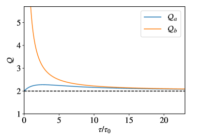
Figure 4: Behaviors of $\mathcal{Q}_{a}$ and $\mathcal{Q}_{b}$, obtained in Eq. (B), as the observation time $\tau$ is varied. The dashed line at $\mathcal{Q}=2$ corresponds to the TUR saturation.

Beyond this specific example, it is difficult to prove in general whether the same inequalities hold for the general Langevin systems. But at least, when the observation time is short ($\tau\ll 1$), we can show that $\mathcal{Q}_{b}\geq\mathcal{Q}_{a}\geq 2$ holds for more general cases involving current-like observables of the form $\mathcal{J}_{\tau}^{\Lambda}(\Gamma)=\int_{0}^{\tau}dt\,\Lambda(x,p)\circ\dot{x}$. Towards this end, we first compute

$$\langle\mathcal{J}_{\tau}^{\Lambda}\rangle=\int_{0}^{\tau}dt\int dxdp\,\frac{s}{m}p\Lambda(x,p)P(x,p,t;s,\omega)\;.$$ (139)

When $\tau\ll 1$, we can use the expansion

$$(\tau\partial_{\tau}-s\partial_{s}-\omega\partial_{\omega})\langle\mathcal{J}_{\tau}^{\Lambda}\rangle$$

$$\quad=\partial_{\tau}[(\tau\partial_{\tau}-s\partial_{s}-\omega\partial_{\omega})\langle\mathcal{J}_{\tau}^{\Lambda}\rangle]\big{|}_{\tau=0}\tau+O(\tau^{2})\;.$$ (140)

Using these, the denominator of the $\mathcal{Q}$ factor satisfies

$$\partial_{\tau}[(\tau\partial_{\tau}-s\partial_{s}-\omega\partial_{\omega})\langle\mathcal{J}_{\tau}^{\Lambda}\rangle]\big{|}_{\tau=0}$$

$$\quad=-\int dxdp\,\Lambda(x,p)\,s(s\partial_{s}+\omega\partial_{\omega})P(x,p,0;s,\omega)\;.$$ (141)

This vanishes when the initial distribution is independent of $s$ and $\omega$; otherwise, it is generally finite. This indicates that the denominator of the $\mathcal{Q}$ factor is $O(\tau^{4})$ in the former case and $O(\tau^{2})$ in the latter. The other observables in the $\mathcal{Q}$ factor typically scale as $\text{Var}(\mathcal{J}_{\tau}^{\Lambda})\sim\tau^{2}$, $\Sigma_{\tau}^{\text{tot}}\sim\tau$, and $\mathcal{B}\sim\tau^{0}$ for $\tau\ll 1$. Combining these scaling behaviors, we obtain $\mathcal{Q}_{a}\sim\tau^{0}$ for nonzero $\mathcal{B}$ and $\mathcal{Q}_{b}\sim\tau^{-1}$ for vanishing $\mathcal{B}$. Thus, when $\tau\ll 1$, we conclude that the TUR with nonzero $\mathcal{B}$ is tighter than the TUR with vanishing $\mathcal{B}$.

References

- Carnot [1824] S. Carnot, Reflections on the motive power of fire, and on machines fitted to develop that power (Bachelier, Paris, 1824).
- Clausius [1879] R. Clausius, The mechanical theory of heat, 2nd ed. (Macmillan & Co., London, 1879).
- Callen [1985] H. B. Callen, Thermodynamics and an Introduction to Thermostatics, 2nd ed. (Wiley, New York, 1985).
- Landauer [1961] R. Landauer, IBM journal of research and development 5, 183 (1961).
- Barato and Seifert [2015] A. C. Barato and U. Seifert, Phys. Rev. Lett. 114, 158101 (2015).
- Gingrich et al. [2016] T. R. Gingrich, J. M. Horowitz, N. Perunov, and J. L. England, Phys. Rev. Lett. 116, 120601 (2016).
- Horowitz and Gingrich [2017] J. M. Horowitz and T. R. Gingrich, Phys. Rev. E 96, 020103 (2017).
- Liu et al. [2020] K. Liu, Z. Gong, and M. Ueda, Phys. Rev. Lett. 125, 140602 (2020).
- Shiraishi [2021] N. Shiraishi, J. Stat. Phys. 185, 19 (2021).
- Dechant and ichi Sasa [2018] A. Dechant and S. ichi Sasa, J. Stat. Mech.: Theor. Exp. 2018, 063209 (2018).
- Hasegawa and Van Vu [2019] Y. Hasegawa and T. Van Vu, Phys. Rev. E 99, 062126 (2019).
- Koyuk and Seifert [2020] T. Koyuk and U. Seifert, Phys. Rev. Lett. 125, 260604 (2020).
- Park and Park [2021] J.-M. Park and H. Park, Phys. Rev. Research 3, 043005 (2021).
- Lee et al. [2021] J. S. Lee, J.-M. Park, and H. Park, Phys. Rev. E 104, L052102 (2021).
- Kwon and Lee [2022] C. Kwon and H. K. Lee, New J. Phys. 24, 013029 (2022).
- Hasegawa [2020] Y. Hasegawa, Phys. Rev. Lett. 125, 050601 (2020).
- Hasegawa [2021] Y. Hasegawa, Phys. Rev. Lett. 126, 010602 (2021).
- Van Vu and Saito [2022] T. Van Vu and K. Saito, Phys. Rev. Lett. 128, 140602 (2022).
- Dechant and Sasa [2018] A. Dechant and S.-i. Sasa, Phys. Rev. E 97, 062101 (2018).
- Brandner and Seifert [2015] K. Brandner and U. Seifert, Phys. Rev. E 91, 012121 (2015).
- Shiraishi et al. [2016] N. Shiraishi, K. Saito, and H. Tasaki, Phys. Rev. Lett. 117, 190601 (2016).
- Shiraishi et al. [2018] N. Shiraishi, K. Funo, and K. Saito, Phys. Rev. Lett. 121, 070601 (2018).
- Van Vu and Hasegawa [2021] T. Van Vu and Y. Hasegawa, Phys. Rev. Lett. 126, 010601 (2021).
- Deffner and Campbell [2017] S. Deffner and S. Campbell, J. Phys. A: Math. Theor. 50, 453001 (2017).
- Nakazato and Ito [2021] M. Nakazato and S. Ito, Phys. Rev. Res. 3, 043093 (2021).
- Dechant [2022] A. Dechant, J. Phys. A: Math. Theor. 55, 094001 (2022).
- Van Vu and Saito [2023] T. Van Vu and K. Saito, Phys. Rev. X 13, 011013 (2023).
- Pietzonka and Seifert [2018] P. Pietzonka and U. Seifert, Phys. Rev. Lett. 120, 190602 (2018).
- Vo et al. [2022] V. T. Vo, T. Van Vu, and Y. Hasegawa, J. Phys. A: Math. Theor. 55, 405004 (2022).
- Vo et al. [2020] V. T. Vo, T. Van Vu, and Y. Hasegawa, Phys. Rev. E 102, 062132 (2020).
- Hasegawa [2023] Y. Hasegawa, Nat. Commun. 14, 2828 (2023).
- [32] S. Lee, D.-K. Kim, J.-M. Park, W. K. Kim, H. Park, and J. S. Lee, arXiv:2207.05961 [cond-mat.stat-mech] .
- Shankar and Marchetti [2018] S. Shankar and M. C. Marchetti, Phys. Rev. E 98, 020604 (2018).
- Dechant and Sasa [2021a] A. Dechant and S.-i. Sasa, Phys. Rev. Res. 3, L042012 (2021a).
- Dechant and Sasa [2021b] A. Dechant and S.-i. Sasa, Phys. Rev. X 11, 041061 (2021b).
- Lee et al. [2022] J. S. Lee, S. Lee, H. Kwon, and H. Park, Phys. Rev. Lett. 129, 120603 (2022).
- Zolotarev [1984] V. M. Zolotarev, Theor. Probab. Appl. 28, 278 (1984).
- Müller [1997] A. Müller, Adv. Appl. Probab. 29, 429–443 (1997).
- Sriperumbudur et al. [2012] B. K. Sriperumbudur, K. Fukumizu, A. Gretton, B. Schölkopf, and G. R. G. Lanckriet, Electron. J. Statist. 6, 1550 (2012).
- Villani [2009] C. Villani, Optimal Transport: Old and New, Vol. 338 (Springer, 2009).
- Santambrogio [2015] F. Santambrogio, Optimal Transport for Applied Mathematicians (Birkäuser Cham, 2015).
- Arjovsky et al. [2017] M. Arjovsky, S. Chintala, and L. Bottou, in Proceedings of the 34th International Conference on Machine Learning, Proceedings of Machine Learning Research, Vol. 70, edited by D. Precup and Y. W. Teh (PMLR, 2017) pp. 214–223.
- [43] A. Dechant and Y. Sakurai, arXiv:1912.08405 [cond-mat.stat-mech] .
- Ito [2023] S. Ito, Info. Geo. 2023, https://doi.org/10.1007/s41884 (2023).
- Lee and Park [2017] J. S. Lee and H. Park, Sci. Rep. 7, 10725 (2017).
- Lee et al. [2019] J. S. Lee, S. H. Lee, J. Um, and H. Park, J. Korean Phys. Soc. 75, 948 (2019).
- Durang et al. [2015] X. Durang, C. Kwon, and H. Park, Phys. Rev. E 91, 062118 (2015).
- Proesmans et al. [2020] K. Proesmans, J. Ehrich, and J. Bechhoefer, Phys. Rev. Lett. 125, 100602 (2020).
- Horowitz [2012] J. M. Horowitz, Phys. Rev. E 85, 031110 (2012).
- Horowitz and Parrondo [2013] J. M. Horowitz and J. M. R. Parrondo, New J. Phys. 15, 085028 (2013).
- Manzano et al. [2015] G. Manzano, J. M. Horowitz, and J. M. R. Parrondo, Phys. Rev. E 92, 032129 (2015).
- Manzano et al. [2018] G. Manzano, J. M. Horowitz, and J. M. R. Parrondo, Phys. Rev. X 8, 031037 (2018).
- Shiraishi and Saito [2019] N. Shiraishi and K. Saito, J. Stat. Phys. 174, 433 (2019).
- Funo et al. [2019] K. Funo, N. Shiraishi, and K. Saito, New J. Phys. 21, 013006 (2019).
- Onsager and Machlup [1953] L. Onsager and S. Machlup, Phys. Rev. 91, 1505 (1953).
- Esposito and Van den Broeck [2010] M. Esposito and C. Van den Broeck, Phys. Rev. Lett. 104, 090601 (2010).
- Seifert [2012] U. Seifert, Rep. Prog. Phys. 75, 126001 (2012).