Auxiliary master equation approach to the Anderson-Holstein impurity problem out of equilibrium
Abstract
We introduce a method based on auxiliary master equation for solving the problem of an impurity with local electron-electron and electron-phonon interaction embedded between two conduction leads with a finite bias voltage. The Anderson-Holstein Hamiltonian is transformed to a corresponding Lindblad equation with a reduced set of sites providing an optimal approximation of the hybridization function. The problem is solved in the superfermion representation using configuration interaction for fermions and bosons. The phonon basis is shifted and rotated with the intention of permitting a low phonon basis cutoff even in the strong-coupling regime. We benchmark this approach with the numerical renormalization group in equilibrium, finding excellent agreement. We observe, however, that the rotation brings no advantage beyond the bare shift. This is even more apparent out of equilibrium, where issues in convergence with respect to the size of the phononic Hilbert space occur only in the rotated basis. As an application of the method, we explore the evolution of the phononic peak in the differential conductance spectra with changing phonon frequency.
I Introduction
Molecular electronics is the endeavor of using single molecules as components in ultra-miniaturized circuits, making use of their particular electronic and vibration properties [1, 2, 3, 4, 5, 6, 7, 8, 9, 10, 11, 12, 13, 14]. Non-equilibrium properties of single molecules can be probed by embedding molecules in gaps between electrodes [15], in mechanically controlled break junctions [16], as well as using scanning tunneling spectroscopy [17, 18]. In these setups it is possible to apply bias voltages that are large compared to characteristic energy scales of the problem, such as inter-level spacing, phonon frequency, and electron-electron repulsion. Spectroscopic measurements are, however, difficult to interpret because the strongly-interacting problems are difficult to solve reliably and accurately out of equilibrium. A number of theoretical tools has been developed in the past [19, 20, 21, 22, 23, 24, 25, 26, 27], but no method has emerged yet as the ultimate solution applicable to all parameter domains.
In this work we present the auxiliary master equation approach for the Anderson-Holstein impurity problem [28, 29, 30, 31, 32, 33]. This Hamiltonian is the minimal description of a molecule with a single low-energy orbital with effective on-site electron-electron repulsion and with the coupling between the on-site charge and the displacement of a local vibration mode, embedded between two metallic conduction leads. The goal is to solve this problem in the regime of sizable electron-electron (e-e) and electron-phonon (e-ph) coupling for large bias voltages and to calculate the differential conductance, which is the main experimentally measurable quantity that provides information on the excitations in the system.
The paper is structured as follows. In Sec. II we start by discussing the basic idea of the auxiliary master equation approach (AMEA). We continue by briefly reviewing our implementation of configuration interaction (CI) for the electrons in Sec. II.5.1, and discuss in more detail the CI treatment of phonons in Sec. II.5.2. In Sec. III we first elaborate on the choice of method parameters. Then we benchmark the conductance against the numerical renormalisation group in equilibrium in Sec. III.2, and show conductance results out of equilibrium in Sec. III.3.
II Model and Method
II.1 Non-equilibrium Green’s functions
We use the Keldysh formalism [34, 35, 36, 37, 38, 39]. The time contour from to and back again leads to a matrix structure for including all time combinations, i.e. both times on the upper contour, one above and one below, etc. Since we are only interested in the steady state, we can take advantage of time translation invariance and fix one time argument of the Green’s functions to zero. This allows us to work directly in the frequency domain instead of time domain. The general form of a Green’s function is then
| (1) |
where . Throughout this paper, underlined quantities represent a structure in Keldysh space. In equilibrium, can be determined from via the fluctuation-dissipation theorem as
| (2) |
with
| (3) |
II.2 Physical impurity model
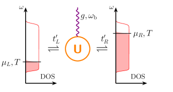
The physical setup consists of an impurity, two electronic reservoirs and one local phonon mode, as depicted in Fig. 1. The respective Hamiltonian may be split up as
| (4) |
is the Hamiltonian of the impurity,
| (5) |
with Hubbard interaction , on-site energy , creation (annihilation) operator () of a fermion at the impurity site with spin , particle number operator , electron-phonon interaction strength , and phonon frequency . The leads are described by
| (6) |
with dispersion and creation (annihilation) operator () of a fermion in the left and right lead, , labeled by momentum . The coupling between the impurity and the bath is given by
| (7) |
where is the coupling strength between the leads and the impurity, and is the number of points. Whenever not mentioned otherwise we have .
Alternatively, the environment may be be described in terms of Green’s functions by defining the hybridization function [40]
| (8) |
where are the Green’s functions of the decoupled leads. (The subscript here stands for “physical”, to distinguish this hybridization function from the auxiliary function to be defined in the next section.) To fully define the problem, one needs to specify the band properties. We chose a flat density of states smoothed around the edges so that
| (9) |
where is the Fermi-Dirac distribution, a fictitious temperature, and the half band-width. The smoothing is introduced to avoid a sharp change that would reduce the quality of reproducing the environment within AMEA; merely quantifies the degree of smoothing. The parameters are set to and throughout this paper. Whenever not mentioned otherwise, the coupling between the reservoir and the impurity is set to (which gives ).
Since the uncoupled leads themselves are in equilibrium, the Keldysh part of their Green’s function can be calculated using the fluctuation-dissipation theorem, Eqs. (2),(3). If not stated otherwise, the chemical potentials of the right and left reservoir are given as , i.e., describes the voltage drop across the impurity.
II.3 Auxiliary impurity model
Since the physical model is defined in an infinitely large Hilbert space, one has to find a way of approximating it for numerical computations on a reduced set of sites. The basic idea of the AMEA is to set the parameters of the Lindblad equation so as to reproduce the physical hybridization function [41].
The Lindblad equation is given as
| (10) |
where is the fermionic creation (annihilation) operator, is the density matrix, and describe the dissipative contributions, and is the unitary part, given as
| (11) |
We define , and the indices and can assume integer values from to , where is the number of bath sites. In this paper we only consider cases in which . This number of bath sites already allows for a large number of parameters, which can be seen when considering that the matrices are only restricted to be positive semidefinite. In other words, the number of parameters used to fit to increases quadratically in . In Ref. 41 it is furthermore explicitly shown that suffices to reproduced a flat density of states accurately.
The part of denoted as is equivalent to . describes the coupling between the auxiliary reservoirs and the impurity, i.e. its parameters are set by . All the other contributions appearing in Eq. (11) are determined in a fitting procedure, which we will discuss in the following.
The auxiliary hybridization function is defined through
| (12) |
where is given [41] by
| (13) |
and as
| (14) |
A note on notation: Bold quantities indicate the structure in the space of auxiliary levels, lower case indicates the decoupled setup, upper case contains the coupling, and the index indicates the non-interacting case.
Given the physical hybridization function , one defines a cost function
| (15) |
which must be minimized to obtain the parameters leading to the optimal approximation of the physical hybridization function.
In this paper we set the weight function to , with . This range suffices to capture the hybridization function appropriately, since our flat density of states ranges from to , and decays exponentially outside this region. A more detailed discussion about the fitting procedure can be found in Ref. 41.
II.4 Superfermion representation
For computational reasons, one may transform the Lindblad equation into the superfermion representation [42]. In this form the Lindbladian becomes a matrix and the density matrix a vector. In this section we will briefly sketch the basic ideas of this procedure, roughly following Ref. [42], see also [43, 44].
We introduce the left vacuum 111The left vacuum is always a left eigenstate with eigenvalue zero for arbitrary Lindbladians in superfermion representation. Furthermore it is important when calculating observables, since it corresponds to taking the trace of the density matrix it is multiplied with. defined as
| (16) |
where and run over all states in the respective Hilbert spaces. Here we doubled the Hilbert space by introducing the ”tilde” space.
Then we apply the density matrix on the left vacuum
| (17) |
This yields a vector in the doubled Hilbert space that contains all information of the density matrix. As the next step, the Lindbladian must also be transformed accordingly. The aim is to replace all density matrices appearing in with . Therefore, we calculate and whenever is next to we can use Eq. (17). To achieve this, one uses the tilde-conjugation rules, given as
| (18) |
since the creation and annihilation operators, once transferred into the tilde space, commute with the density matrix 222The density matrix has an even number of normal-space operators. and anticommute (fermionic) or commute (bosonic) with the normal-space operators. The Lindbladian then takes the form
| (19) |
with the matrix
| (20) |
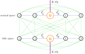
where , and . As defined in Sec. II.3, the impurity site is indexed . Fig. 2 shows the Lindblad setup in its superfermion form 333Ref. 41 shows that under usage of all available parameters, as is the case here, the geometry has no influence on the result. This justifies our choice here., where the blue lines represent the unitary contributions () and the green ones the dissipative contributions (). Furthermore, since the Lindbladian in Eq. (19) is not a superoperator anymore, it does not carry the double hat. This also allows to easily distinguish between superoperators and operators in superfermion space.
As can be deduced from Eq. (19), normal and tilde fermionic particles are always created and annihilated simultaneously, therefore their difference is conserved, i.e.,
| (21) |
This is valid for both spins separately, since angular momentum is also conserved.
Since the left vacuum is always a left eigenstate of the Lindbladian with eigenvalue zero, it lies in the subspace . This can be observed from Eq. (16), since all fermionic states have by definition the same number of normal and tilde electrons. Since the corresponding right eigenvector is the steady state, it is restricted to the same subspace.
The fermionic Green’s functions can be expressed in the Lehmann representation. For positive times () the greater () and lesser () component are given as
| (22) |
where and are the left and right eigenvectors of the Lindbladian and the corresponding eigenvalues. From this all other fermionic Green’s functions of interest, as well as the self energy (), can be obtained:
| (23) |
For bosonic Green’s functions there exist similar expressions as Eqs. (22) and (23). Computationally, we calculate the steady state using the biconjugate gradient method, and the Green’s function using the Bi-Lanczos scheme [48]. The basis used to express is obtained as described in the next section.
II.5 Configuration Interaction
The most straightforward basis choice for is in terms of and operators. Then one can perform the calculation using the full many-body Lindbladian using a cutoff in the number of included phonons. The resulting matrix grows exponentially in the system size , therefore we rotate the bosonic and fermionic single particle operators with the aim of cutting off the fermionic states in a controlled way, and obtaining a reduced cutoff in the bosonic states. This is discussed in the following subsections, where we roughly follow Ref. 49.
II.5.1 Electrons
The treatment of electrons in the AMEA using CI is explained in detail in Ref. 50. Here we will only give a brief overview of the main steps. We start by defining
| (24) |
where and . Here (and thereby ) takes into account the electron-electron and electron-phonon (the origin of the phononic term will become clear in the following, see Sec. II.5.2) interaction on a mean field level.
The matrix is in principle the same for both spins, since there is no magnetic term in the Lindbladian. We showed in Ref. 50 that choosing a spin-dependent (magnetised) Hartree-Fock term reduces the error originating from the basis cutoff we introduce within CI. The respective mean field (Hartree-Fock) Lindbladian reads
| (25) |
In our previous paper we fixed and to introduce an artificial magnetisation. The exact values for do not have a strong influence on the shape of the impurity Green’s function, as long as it is far enough from , but not too far (roughly in the range 0.6-0.9). Since not all the results we show here are particle-hole symmetric, we compute the total Hartree-Fock electron occupation self-consistently using Eq. (25) and introduce a magnetisation as , .
The non-Hermitian matrix can be diagonalised straightforwardly as
| (26) |
where () are the right (left) eigenvectors of , and its eigenvalues. In this basis, the Hartree-Fock Lindbladian reads
| (27) |
The new operators are defined as and , which obey fermionic anticommutation relations. However, the creation and annihilation operators are not hermitian conjugates of each other, i.e. .
The steady state of the non-interacting Lindbladian can be found by identifying which operators annihilate it. In other words, we must have
| (28) |
because anything else would imply a divergent state, as becomes apparent when considering
| (29) |
For computational reasons we furthermore perform a particle-hole transformation
| (30) |
with components
| (31) |
From this we get . Starting from the Hartree-Fock steady state as a reference state, we can create a subspace of excited states by applying operator pairs,
| (32) |
which is equivalent to
| (33) |
with and taking all values resulting in non-vanishing states, which obey the conservation rules, namely , where is a spin-dependent constant. For the steady state we have and for the Green’s functions and .
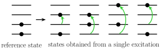
The state in Eq. (32) corresponds to a single ”particle-hole” excitation, and can be graphically interpreted as depicted in Fig. 3 (shown in the basis). By applying more such pairs in sequence, one obtains higher excitations. In this paper we always use a basis created by up to three particle-hole excitations (referred to in the literature as CISDT).
Eventually Eq. (19) is transformed into the basis, such that the fermionic contributions to the matrix elements in the many-body Lindblad matrix can be calculated in this subspace.
II.5.2 Phonons
When including phonons, the Hilbert space becomes in principle infinite, so that one has to introduce a cutoff in the maximum phonon number. The larger the cutoff, the better the approximation for observables, but at the cost of higher memory usage and longer computation times. By choosing an advantageous single particle basis, the number of bosonic particles can be kept low while still obtaining accurate results.
One starts by introducing an offset to the bosonic operators, which corresponds to the NECI* shift introduced in Ref. [49], whose treatment we roughly follow below. This shifts the number of phonons in the new vacuum to the amount corresponding to the mean-field electron occupation, i.e., without taking into account the effect of electronic fluctuations:
| (34) |
The corresponding Lindblad term in the superfermion representation then reads
| (35) |
In the next step one ”rotates” the phononic basis, i.e., one introduces a linear transformation between the ”tilde” and ”non-tilde” phononic creation and annihilation operator, as first introduced in Ref. 49. This transformation is obtained by the exact solution of an auxiliary Lindblad equation acting on the isolated phonon level
| (36) |
this equation can be obtained exactly by eliminating the “fermionic reservoir” from the isolated phonon level within the weak-coupling () regime with the Born-Markov-Secular approximation [51, 52]. In this case, the ratio can be written in terms a suitable fermionic density density correlation function, and in the equilibrium case can be inferred from the relation
| (37) |
With this we rewrite the impurity Lindbladian as
| (38) |
with being the superfermion version of given as
| (39) |
contains the mean-field on-site energies felt by the electrons due to the e-e and e-ph coupling and considers the thermalization effect the electrons have on the phonons. then contains corrections beyond the mean-field level felt by the electrons, as well as corrections to the thermalization effect the electrons have on the phonons.
In the case of the electrons, we used the matrices diagonalising to transform the electronic single particle operators. For the phonons we proceed in a similar way, where we start by rewriting
| (40) |
where
| (41) |
and are the right eigenvectors of . For convenience we define
| (42) |
such that
| (43) |
In the -basis the Lindbladian is diagonal, therefore the steady state is given by a single Fock state, which is simultaneously the vacuum in this basis () 444Also the left vacuum becomes the vacuum, i.e. , which it remains for arbitrary Lindbladians in this basis.. This state contains the thermalizing effect the electrons have on the phonons, making it a good choice for a reference state 555Which is of importance if one restricts the Hilbert space, otherwise any arbitrary reference state would be equally good. to build the phononic basis from:
| (44) |
We define the cutoff value for the number of included phonons per site as ”” (Number of phonons), i.e., , with integers. To transform Eq. (35) in the basis we use
| (45) |
which follows from Eqs. (40) and (42). With this in its final version reads
| (46) |
III Results
.
III.1 Method parameters
In equilibrium, the parameters and can be calculated straightforwardly from the temperature of the system. Only the ratio appears in equations, thus there is actually a single free parameter that is fixed by . Out of equilibrium, we need to choose an effective temperature felt by the phonons, which is, however, not defined unambiguously. Two approaches were considered: a) fitting the Fermi function () to the non-equilibrium distribution (), b) enforcing . Comparing the results obtained from both procedures showed that fitting works better. Here we calculate the non-equilibrium distribution from Eq. (25), i.e., for the mean-field case. This is computationally much less costly than performing an iterative many-body calculation to obtain this parameter.
III.2 Comparison with the NRG in equilibrium
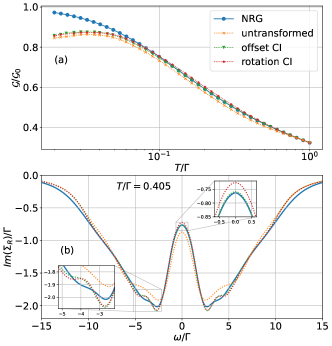
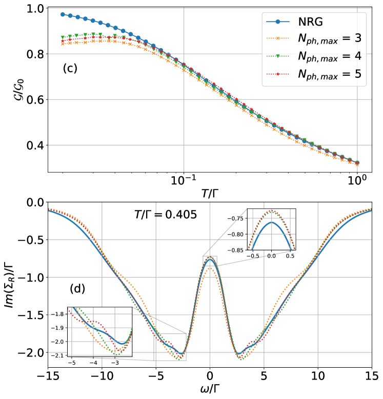
As a benchmark of the approach presented here, we compare our results with NRG in the equilibrium case, where the latter is known to be very accurate, especially in the low-energy regions. First, we investigate how the transformation of the phononic basis introduced in Sec. II.5.2 affects the accuracy of the calculation. More specifically, we compare the results obtained without any transformation, with only the offset (”offset CI”), Eq. (34), and with both, the offset and the rotation (”rotation CI”), Eqs. (45) and (34). We plot the zero-bias conductance as a function of temperature, which gives us insight into the effect of the transformations at low energies over a wide temperature range. While the conductance mainly probes the low-energy region, we address higher energies by evaluating . From the Meir-Wingreen formula [55] one obtains the conductance as
| (47) |
for the case of proportional coupling. Here, are also referred to as the ”lead self-energies”. We have unless otherwise specified (this follows from our definition of in eq. (9) and our default values for , as given in Sec. II.2).
The Numerical Renormalization Group (NRG) [56, 57, 58] is well known for capturing the equilibrium properties very accurately. Therefore, we use the results obtained from NRG Ljubljana 666http://nrgljubljana.ijs.si/ as a reference for the equilibrium case 777The NRG calculations have been performed using the discretization parameter , with twist averaging over four discretization grids, keeping up to 10000 spin multiplets in truncation, and using broadening parameter . The final spectral functions have been computed using the self-energy trick.. Both the offset CI and the rotation CI results compare very well with NRG and perform significantly better than the results obtained without any transformation, as can be seen in the conductance results in Fig. 4(a). Considering a maximum allowed deviation of 3% with respect to the NRG, temperatures down to 0.05 can be reached for with both CI transformations. The offset CI performs marginally better.
The self energies of the offset and rotation CI are also almost on top of each other, see Fig. 4(b). They mostly coincide with the NRG self energy, except close to the phononic feature, which is more pronounced for the CI methods. We have compared the self energies at a temperature which is close to the one obtained for non-equilibrium at , using the procedure discussed in Sec. III.1.
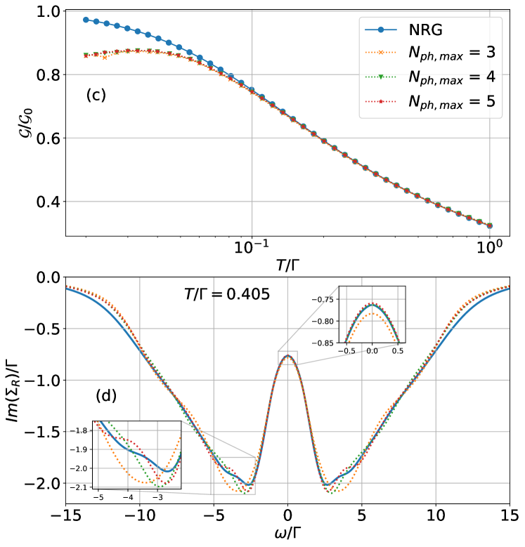
With increasing phonon cutoff, we expect convergence of all observables. We investigate the cutoff dependence by again plotting the zero-bias conductance as a function of temperature as well as the self energy, see Fig. 5. The plots shows that the convergence behavior of the offset CI at low energies is superior. In the self energy, however, close to the phononic feature both approaches have trouble reaching full convergence.
III.3 Non-equilibrium results
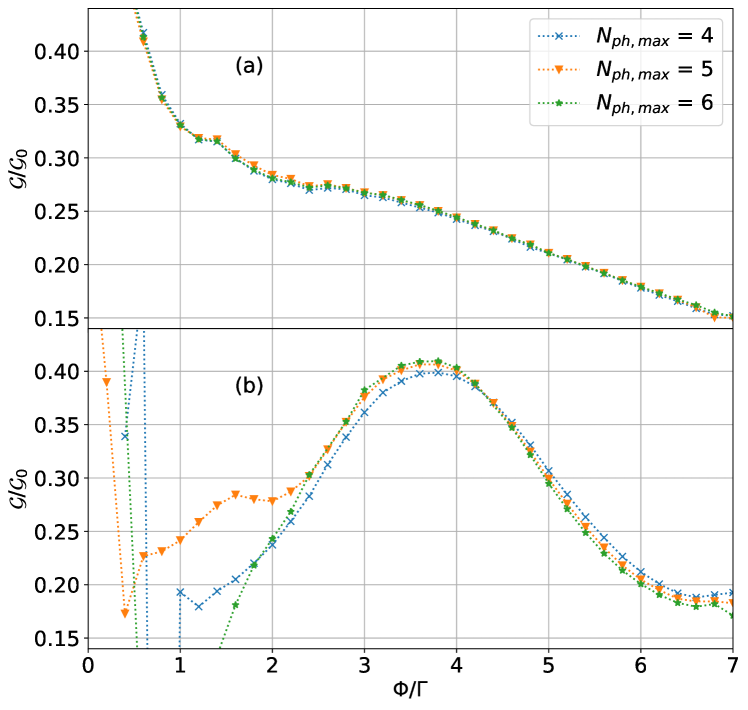
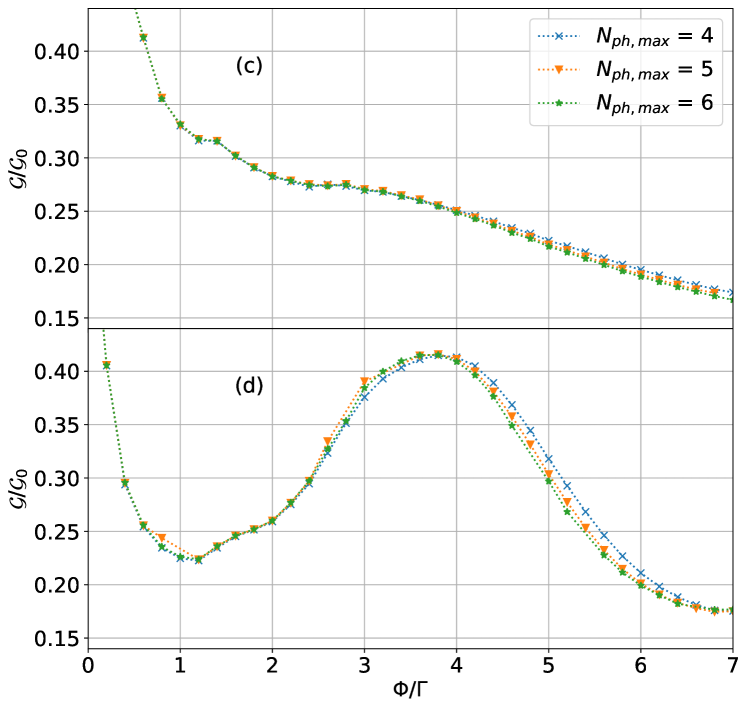
Having shown that in equilibrium the offset CI performs better than the rotation CI, especially at low energies, we now study if this is the case also in non-equilibrium. We consider the differential conductance as a function of applied voltage, and start by investigating the convergence behavior as a function of the number of included phonons. We considered several values of the system-environment coupling () which we describe in terms of (see Eq. (47)) for easier notation. Decreasing is observed to give rise to a phononic feature at the phonon frequency.
Both transformations converge rapidly for stronger system-environment coupling. In the case of weaker coupling, which is when the phononic feature appears, the rotation CI fails at low voltages, and does not converge at the phonon frequency. The offset CI on the other hand converges almost immediately over the full voltage range. Therefore, especially in non-equilibrium, the rotation does not prove to be advantageous. We expect that a (possibly partial) Lang-Firsov transformation [61, 62, 63] would bring improvements; this will be implemented in future work.
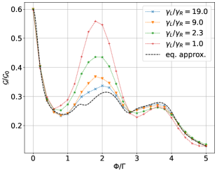
We also investigated the transition from very asymmetric lead coupling () to the symmetric case. We use the offset CI here, since it proved to be superior to the rotation CI. For , the finite-bias conductance can be obtained using from a zero-bias calculation888This can be seen in the following way: In general, changing the voltage leads to a different Keldysh component of the hybridization function, which then alters at the impurity. However, provided the lead in which the chemical potential is changed is weakly coupled, does not change with , and consequently neither does . Then the second term in Eq. (47) becomes zero, and the first only contains .. Figure 7 shows the nonlinear conductance for a range of using the offset CI. The finite bias is applied by choosing and . For large asymmetry we see that the conductance is very close to the one obtained by the equilibrium approximation with . As we approach equal coupling of the leads, the non-equilibrium effects become apparent and the shape of the conductance curve changes significantly. The vibrational features are expected at , while the Coulomb peak is expected at [65, 19, 24].
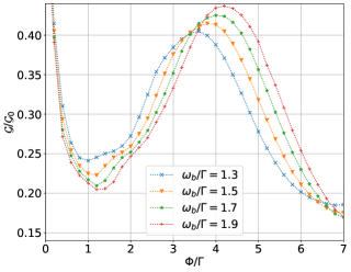
Finally, we investigate the effect the phonon frequency has on the phononic feature in the fermionic spectrum, as well as on the Hubbard peak. Again we use the offset CI. Figure 8 shows that the feature moves with , as one would expect, and that it is slowly ”absorbed” in the Hubbard peak. The Hubbard peak itself is shifted to higher bias, since increasing decreases the phononic attraction felt by the electrons.
In conclusion, we showed that the method discussed in Ref. [49] doesn’t seem to provide any improvement of the accuracy of the CI calculation with respect to a simple shift in the phononic operators. This is the case especially in non-equilibrium, but also in equilibrium where the phonons have a well-defined temperature. Nevertheless, the equilibrium results presented coincide well with NRG, and the offset CI converges well in non-equilibrium as the phononic Hilbert space is increased.
IV Conclusion
We have presented a solver for the Anderson-Holstein problem out of equilibrium. After mapping the Hamiltonian to an auxiliary impurity model in the form of a Lindblad equation and passing to the superfermion representation, we tackled the resulting problem using configuration interaction approach. In the electron sector we use a basis extending up to three particle-hole excitations, while in the phonon sector we attempted to optimize the basis using a shift and rotation, as introduced in Ref [49]. The method was benchmarked against the numerical renormalization group results in equilibrium, then tested out of equilibrium. We find that in equilibrium the shift as well as the additional rotation allow for high accuracy, using only a small phononic Hilbert space. However, the rotation as discussed in Ref. [49], any advantage beyond purely shifting the operators, and in some cases it even introduces instabilities. Therefore, taking into account the effects of the fluctuationg fermionic density on the phonon field doesn’t seem to provide any advantage in the parameter region we have been considering. This becomes even more apparent in non-equilibrium, where the rotation leads to convergence problems in the number of phonons for some parameter regimes. Using the shifted operators, on the other hand, gives quickly converging results. We also use the offset CI to show the propagation of the phononic feature, as well as the Hubbard peak, due to changing phonon frequency. Our solver is thus capable of tackling the problem in the very demanding regime of large bias and strong interactions using only a shift in the phononic operators. Further improvements would consist of implementing the Lang-Firsov transformation. This could potentially lead to a capable solver for interpreting experimental bias spectra.
Acknowledgements.
This research was funded by the Austrian Science Fund (Grant No. P 33165-N) and by NaWi Graz. The results have been obtained using the Vienna Scientific Cluster and the L/A-Cluster Graz. To compute the many-body Lindblad matrix we use the QuSpin library [66]References
- Jaklevic and Lambe [1966] R. C. Jaklevic and J. Lambe, Molecular vibration spectra by electron tunneling, Phys. Rev. Lett. 17, 1139 (1966).
- Lambe and Jaklevic [1968] J. Lambe and R. C. Jaklevic, Molecular vibration spectra by inelastic electron tunneling, Phys. Rev. 165, 821 (1968).
- Aviram and Ratner [1974] A. Aviram and M. A. Ratner, Molecular rectifiers, Chem. Phys. Lett. 29, 277 (1974).
- Reed et al. [1997] M. A. Reed, C. Zhou, C. J. Muller, T. P. Burgin, and J. M. Tour, Conductance of a molecular junction, Science 278, 252 (1997).
- Chen et al. [1999] J. Chen, M. A. Reed, A. M. Rawlett, , and J. M. Tour, Large on-off ratios and negative differential resistance in a molecular electronic device, Science 286, 1550 (1999).
- Nitzan [2001] A. Nitzan, Electron transmission through molecules and molecular interfaces, Ann. Rev. Phys. Chem. 52, 681 (2001).
- Donhauser et al. [2001] Z. J. Donhauser, B. A. Mantooth, K. F. Kelly, L. A. Bumm, J. D. Monnell, J. J. Stapleton, D. W. P. Jr., A. M. Rawlett, D. L. Allara, J. M. Tour, and P. S. Weiss, Conductance switching in single molecule through conformational changes, Science 292, 2303 (2001).
- Zhitenev et al. [2002] N. B. Zhitenev, H. Meng, and Z. Bao, Conductance of small molecular junctions, Physical Review Letters 88, 10.1103/physrevlett.88.226801 (2002).
- Qiu et al. [2003] X. H. Qiu, G. V. Nazin, and W. Ho, Vibrationally resolved fluorescence excited with submolecular precision, Science 299, 542 (2003).
- Yu et al. [2004] L. H. Yu, Z. K. Keane, J. W. Ciszek, L. Cheng, M. P. Stewart, J. M. Tour, and D. Natelson, Inelastic electron tunneling via molecular vibrations in single-molecule transistors, Phys. Rev. Lett. 93, 266802 (2004).
- Galperin et al. [2007a] M. Galperin, M. A. Ratner, and A. Nitzan, Molecular transport junctions: vibrational effects, J. Phys.: Condens. Matter 19, 103201 (2007a).
- Zimbovskaya and Pederson [2011] N. A. Zimbovskaya and M. R. Pederson, Electron transport through molecular junctions, Physics Reports 509, 1 (2011).
- Song et al. [2011] H. Song, M. A. Reed, and T. Lee, Single molecule electronic devices, Adv. Materials 23, 1583 (2011).
- Aradhya and Venkataraman [2013] S. V. Aradhya and L. Venkataraman, Single-molecule junctions beyond electronic transport, Nature Nanotechnology 8, 399 (2013).
- Park et al. [2000] H. Park, J. Park, A. K. L. Lim, E. H. Anderson, A. P. Alivisatos, and P. L. McEuen, Nanomechanical oscillations in a single-c60 transistor, Nature 407, 57 (2000).
- Agraït et al. [2003] N. Agraït, A. L. Yeyati, and J. M. van Ruitenbeek, Quantum properties of atomic-sized conductors, Phys. Rep. 377, 81 (2003).
- Stipe et al. [1998] B. C. Stipe, M. A. Rezaei, and W. Ho, Single-molecule vibrational spectroscopy and microscopy, Science 280, 1732 (1998).
- Moresco [2004] F. Moresco, Manipulation of large molecules by low-temperature stm: model systems for molecular electronics, Phys. Rep. 399, 175 (2004).
- Paaske and Flensberg [2005] J. Paaske and K. Flensberg, Vibrational sidebands and the kondo effect in molecular transistors, Physical Review Letters 94, 10.1103/physrevlett.94.176801 (2005).
- Picano et al. [2023] A. Picano, F. Grandi, P. Werner, and M. Eckstein, Stochastic semiclassical theory for nonequilibrium electron-phonon coupled systems, Phys. Rev. B 108, 035115 (2023).
- Galperin et al. [2007b] M. Galperin, A. Nitzan, and M. A. Ratner, Inelastic effects in molecular junctions in the coulomb and kondo regimes: Nonequilibrium equation-of-motion approach, Physical Review B 76, 10.1103/physrevb.76.035301 (2007b).
- Werner and Millis [2007] P. Werner and A. J. Millis, Efficient dynamical mean field simulation of the holstein-hubbard model, Phys. Rev. Lett. 99, 146404 (2007).
- Eickhoff et al. [2020] F. Eickhoff, E. Kolodzeiski, T. Esat, N. Fournier, C. Wagner, T. Deilmann, R. Temirov, M. Rohlfing, F. S. Tautz, and F. B. Anders, Inelastic electron tunneling spectroscopy for probing strongly correlated many-body systems by scanning tunneling microscopy, Phys. Rev. B 101, 125405 (2020).
- Roura-Bas et al. [2013] P. Roura-Bas, L. Tosi, and A. A. Aligia, Nonequilibrium transport through magnetic vibrating molecules, Physical Review B 87, 10.1103/physrevb.87.195136 (2013).
- Roura-Bas et al. [2016] P. Roura-Bas, L. Tosi, and A. A. Aligia, Replicas of the kondo peak due to electron-vibration interaction in molecular transport properties, Phys. Rev. B 93, 115139 (2016).
- Laakso et al. [2014] M. A. Laakso, D. M. Kennes, S. G. Jakobs, and V. Meden, Functional renormalization group study of the anderson–holstein model, New Journal of Physics 16, 023007 (2014).
- Chen et al. [2020] F. Chen, M. I. Katsnelson, and M. Galperin, Nonequilibrium dual-boson approach, Phys. Rev. B 101, 235439 (2020).
- Holstein [1959] T. Holstein, Studied of polaron motion: Part i. the molecular-crystal model, Ann. Phys. 8, 325 (1959).
- Anderson [1961] P. W. Anderson, Localized magnetic states in metals, Phys. Rev. 124, 41 (1961).
- Newns [1969] D. M. Newns, Self-consistend model of hydrogen chemisorption, Phys. Rev. 178, 1123 (1969).
- Jeon et al. [2003] G. S. Jeon, T.-H. Park, and H.-Y. Choi, Numerical renormalization-group study of the symmetric Anderson-Holstein model: Phonon and electron spectral functions, Phys. Rev. B 68, 045106 (2003).
- Hewson and Meyer [2002] A. C. Hewson and D. Meyer, Numerical renormalization group study of the anderson-holstein model, J. Phys. - Condens. Mat. 14, 427 (2002).
- Cornaglia et al. [2004] P. S. Cornaglia, H. Ness, and D. R. Grempel, Many-body effects on the transport properties of single-molecule devices, Phys. Rev. Lett. 93, 147201 (2004).
- Schwinger [1961] J. Schwinger, Brownian motion of a quantum oscillator, J. Math. Phys. 2, 407 (1961).
- Kadanoff and Baym [1962] L. P. Kadanoff and G. Baym, Quantum Statistical Mechanics: Green’s Function Methods in Equilibrium and Nonequilibrium Problems (Addison-Wesley, Redwood City, CA, 1962).
- Keldysh [1965] L. V. Keldysh, Diagram technique for nonequilibrium processes, Sov. Phys. JETP 20, 1018 (1965).
- Rammer and Smith [1986] J. Rammer and H. Smith, Quantum field-theoretical methods in transport theory of metals, Rev. Mod. Phys. 58, 323 (1986).
- Haug and Jauho [1998] H. Haug and A.-P. Jauho, Quantum Kinetics in Transport and Optics of Semiconductors (Springer, Heidelberg, 1998).
- Wagner [1991] M. Wagner, Expansions of nonequilibrium green’s functions, Phys. Rev. B 44, 6104 (1991).
- Economou [2006] E. N. Economou, Green’s Functions in Quantum Physics (Springer, Heidelberg, 2006).
- Dorda et al. [2017] A. Dorda, M. Sorantin, W. von der Linden, and E. Arrigoni, Optimized auxiliary representation of non-markovian impurity problems by a lindblad equation, New J. Phys. 19, 063005 (2017).
- Dzhioev and Kosov [2011] A. A. Dzhioev and D. S. Kosov, Super-fermion representation of quantum kinetic equations for the electron transport problem, J. Chem. Phys. 134, 044121 (2011).
- Dorda et al. [2014] A. Dorda, M. Nuss, W. von der Linden, and E. Arrigoni, Auxiliary master equation approach to non – equilibrium correlated impurities, Phys. Rev. B 89, 165105 (2014).
- Arrigoni and Dorda [2018] E. Arrigoni and A. Dorda, Master equations versus keldysh green’s functions for correlated quantum systems out of equilibrium, in Out-of-Equilibrium Physics of Correlated Electron Systems, Springer Series in Solid-State Sciences, Vol. 191, edited by R. Citro and F. Mancini (Springer International Publishing, Cham, Switzerland, 2018) Chap. 4, pp. 121–188.
- Note [1] The left vacuum is always a left eigenstate with eigenvalue zero for arbitrary Lindbladians in superfermion representation. Furthermore it is important when calculating observables, since it corresponds to taking the trace of the density matrix it is multiplied with.
- Note [2] The density matrix has an even number of normal-space operators.
- Note [3] Ref. \rev@citealpdo.so.17 shows that under usage of all available parameters, as is the case here, the geometry has no influence on the result. This justifies our choice here.
- C. [1950] L. C., An Iteration Method for the Solution of the Eigenvalue Problem of Linear Differential and Integral Operators., Journal of Research of the National Bureau of Standards 45, 255 (1950).
- Dzhioev and Kosov [2014] A. A. Dzhioev and D. S. Kosov, Nonequilibrium configuration interaction method for transport in correlated quantum systems, Journal of Physics A: Mathematical and Theoretical 47, 095002 (2014).
- Werner et al. [2023] D. Werner, J. Lotze, and E. Arrigoni, Configuration interaction based nonequilibrium steady state impurity solver, Phys. Rev. B 107, 075119 (2023).
- Schaller [2014] G. Schaller, Open Quantum Systems Far from Equilibrium, Lecture notes in physics (Springer, Heidelberg, 2014).
- Breuer and Petruccione [2009] H.-P. Breuer and F. Petruccione, The Theory of Open Quantum Systems (Oxford University Press, Oxford, England, 2009).
- Note [4] Also the left vacuum becomes the vacuum, i.e. , which it remains for arbitrary Lindbladians in this basis.
- Note [5] Which is of importance if one restricts the Hilbert space, otherwise any arbitrary reference state would be equally good.
- Meir and Wingreen [1992] Y. Meir and N. S. Wingreen, Landauer formula for the current through an interacting electron region, Phys. Rev. Lett. 68, 2512 (1992).
- Wilson [1975] K. G. Wilson, The renormalization group: Critical phenomena and the kondo problem, Rev. Mod. Phys. 47, 773 (1975).
- Bulla et al. [2008] R. Bulla, T. A. Costi, and T. Pruschke, Numerical renormalization group method for quantum impurity systems, Rev. Mod. Phys. 80, 395 (2008).
- Zitko and Pruschke [2009] R. Zitko and T. Pruschke, Energy resolution and discretization artefacts in the numerical renormalization group, Phys. Rev. B 79, 085106 (2009).
- Note [6] Http://nrgljubljana.ijs.si/.
- Note [7] The NRG calculations have been performed using the discretization parameter , with twist averaging over four discretization grids, keeping up to 10000 spin multiplets in truncation, and using broadening parameter . The final spectral functions have been computed using the self-energy trick.
- Koch et al. [2011] T. Koch, J. Loos, A. Alvermann, and H. Fehske, Non – equilibrium transport through molecular junctions in the quantum regime, Phys. Rev. B 84, 125131 (2011).
- Loos et al. [2009] J. Loos, T. Koch, A. Alvermann, A. R. Bishop, and H. Fehske, Phonon affected transport through molecular quantum dots, J. Phys. Condens. Matter 21, 395601 (2009).
- Hohenadler and von der Linden [2007] M. Hohenadler and W. von der Linden, Lang – firsov approaches to polaron physics: From variational methods to unbiased quantum monte carlo simulations, in Polarons in Advanced Materials, Springer Series in Materials Science, Vol. 103, edited by A. S. Alexandrov (Canopus/Springer Publishing, 2007).
- Note [8] This can be seen in the following way: In general, changing the voltage leads to a different Keldysh component of the hybridization function, which then alters at the impurity. However, provided the lead in which the chemical potential is changed is weakly coupled, does not change with , and consequently neither does . Then the second term in Eq. (47\@@italiccorr) becomes zero, and the first only contains .
- Mitra et al. [2004] A. Mitra, I. Aleiner, and A. J. Millis, Phonon effects in molecular transistors: Quantal and classical treatment, Physical Review B 69, 10.1103/physrevb.69.245302 (2004).
- Weinberg et al. [2023] P. Weinberg, M. Schmitt, and M. Bukov, Computer simulations, http://quspin.github.io/QuSpin/ (2023), [Online; accessed Oct-2023].