Max $s,t$-Flow Oracles and Negative Cycle Detection
in Planar Digraphs

Abstract

We study the maximum $s,t$-flow oracle problem on planar directed graphs where the goal is to design a data structure answering max $s,t$-flow value (or equivalently, min $s,t$-cut value) queries for arbitrary source-target pairs $(s,t)$. For the case of polynomially bounded integer edge capacities, we describe an exact max $s,t$-flow oracle with truly subquadratic space and preprocessing, and sublinear query time. Moreover, if $(1-\epsilon)$-approximate answers are acceptable, we obtain a static oracle with near-linear preprocessing and $\widetilde{O}(n^{3/4})$ query time and a dynamic oracle supporting edge capacity updates and queries in $\widetilde{O}(n^{6/7})$ worst-case time.

To the best of our knowledge, for directed planar graphs, no (approximate) max $s,t$-flow oracles have been described even in the unweighted case, and only trivial tradeoffs involving either no preprocessing or precomputing all the $n^{2}$ possible answers have been known.

One key technical tool we develop on the way is a sublinear (in the number of edges) algorithm for finding a negative cycle in so-called dense distance graphs. By plugging it in earlier frameworks, we obtain improved bounds for other fundamental problems on planar digraphs. In particular, we show:

1. a deterministic $O(n\log(nC))$ time algorithm for negatively-weighted SSSP in planar digraphs with integer edge weights at least $-C$. This improves upon the previously known bounds in the important case of weights polynomial in $n$.

2. an improved $O(n\log{n})$ bound on finding a perfect matching in a bipartite planar graph.

1 Introduction

Single-source shortest paths (with negative weights allowed) and maximum flow are among the most fundamental computational problems on directed graphs. The best known strongly polynomial $\widetilde{O}(nm)$ time bounds for these problems [Bel58, FJ56, GN80, ST83] have stood for decades. The scaling framework [EK72, Gab85] made it apparent that this quadratic barrier can be overcome in a relaxed weakly polynomial model, where the magnitude $\log{C}$ of the largest numeric value $C$ (such as the maximum absolute weight/capacity of an edge) is also used to measure the size of an instance. That is, a graph algorithm is weakly polynomial-time if it runs in time polynomial in $n$, $m$, and $\log{C}$. Weakly polynomial-time algorithms typically assume integer data to guarantee that exact solutions are computed. In particular, [Gab85] showed an $O(mn^{3/4}\log{C})$ algorithm for single-source shortest paths with integer weights (and more general problems such as minimum-cost bipartite matching). That method has been subsequently refined to run in time $\widetilde{O}(m\sqrt{n}\log{C})$ [GT89, Gol95]. Later, a similar subquadratic bound has been obtained also for the maximum flow problem by Goldberg and Rao [GR98]. These algorithms, developed in the previous century, remain the best deterministic combinatorial algorithms for these problems to date.

Recent years have brought impressive progress on single-source shortest paths and maximum flow in the weakly polynomial regime with integer data. The usage of the interior-point method (IPM) for solving linear programs [Kar84] along with dynamic algebraic data structures proved very powerful for solving fundamental polynomial-time graph problems and ultimately led to very efficient ${\widetilde{O}((m+n^{3/2})\log{C})}$ [vdBLL⁺21] and $O(m^{1+o(1)}\log^{2}{C})$ time [CKL⁺22, vdBCK⁺23] algorithms for the minimum-cost flow problem, which generalizes both the SSSP and maximum flow problems. Even more recently, [BNW22] developed a randomized algorithm for the negatively-weighted SSSP problem exclusively that is purely combinatorial in nature and runs (with the tweaks of [BCF23] applied) in $O(m\log^{2}{n}\log{(nC)}\log\log{n})$ expected time.

The focus of this paper is on algorithms for planar digraphs. Planarity-exploiting near-optimal strongly polynomial algorithms have been known for both single-source shortest paths and maximum flow. Fakcharoenphol and Rao [FR06] gave the first near-optimal $O(n\log^{3}{n})$-time algorithm for negative cycle detection and SSSP in planar digraphs. This has been subsequently improved by [KMW10, MW10] and the current best known bound is $O(n\log^{2}{n}/\log\log{n})$. Maximum $s,t$-flow on planar digraphs can be computed in $O(n\log{n})$ time [BK09, Eri10]. The multiple-source multiple-sink case of max-flow is not easily reducible to the single-source single-sink case while preserving planarity, and the best known upper bound for that case is $O(n\log^{3}{n})$ [BKM⁺17]. All these state-of-the-art algorithms for planar graphs are combinatorial and deterministic.

Since planarity enables efficient strongly polynomial algorithms for shortest paths and maximum flow, the study of weakly polynomial-time algorithms for these problems in the planar case has been rather limited. To the best of our knowledge, the combinatorial scaling framework has only been applied to unit-capacity minimum-cost flow problems on planar graphs [AKLR20, KS19, LR19], but the achieved bounds were still a polynomial factor away from linear. Recently, an algebraic IPM-based near-linear randomized algorithm for planar min-cost flow has been proposed [DGG⁺22].

In this paper we apply the combinatorial scaling framework to the maximum $s,t$-flow oracle problem and the negative-weights single-source shortest paths problem on planar digraphs.

1.1 Our contribution

1.1.1 Max $s,t$-flow oracles

We consider the following max $s,t$-flow oracle problem. Given a planar digraph ${G=(V,E)}$, preprocess it into a data structure supporting max $s,t$-flow value (or, equivalently, min $s,t$-cut capacity) queries for arbitrary pairs $s,t\in V\times V$. One extreme trivial solution for this problem is to skip preprocessing and answer queries using the state-of-the-art $O(n\log{n})$-time max $s,t$-flow algorithms for planar digraphs [BK09, Eri10]. Another extreme approach is to store all the possible $O(n^{2})$ answers and read the stored result in $O(1)$ time upon query. [ŁNSW12] showed that computing all-pairs max $s,t$-flow values in planar graphs takes near-optimal $\widetilde{O}(n^{2})$ time. They also showed that in planar digraphs there might be $\Theta(n^{2})$ distinct max $s,t$-flow values (as opposed to general undirected graphs, where there may be at most $n-1$ max-flow values) and asked whether constant-time queries are possible after subquadratic preprocessing. Nussbaum [Nus14, Section 9.1.3] relaxed this open question and asked whether sublinear query time is possible after subquadratic preprocessing. Of course, ideally, we would like to support queries in $\widetilde{O}(1)$ time after $\widetilde{O}(n)$-time preprocessing. This is in fact possible in undirected planar graphs [BSW15], where min $s,t$-cuts have much more convenient structure compared to directed planar graphs. However, for the directed case, no non-trivial preprocessing/query tradeoffs have been described to date even for the case when the input graph is unweighted and/or we only seek constant-factor approximate query answers.

First of all, we give an affirmative answer to the open problem posed in [Nus14] in the important case of integer weights which also covers unweighted graphs.

Theorem 1.1.

Let $G=(V,E)$ be a planar digraph with integer edge capacities in $[1,C]$ and let $r\in[1,n]$. In $\widetilde{O}(nr)$ time one can construct an $\widetilde{O}(nr)$-space data structure that, for any query pair $(s,t)\in V\times V$, computes the max $s,t$-flow (or min $s,t$-cut) value in $G$ in $\widetilde{O}(n^{3/2}/r^{3/4}\cdot\log^{2}{C})$ time.

Note that the data structure of Theorem 1.1 achieves both truly subquadratic preprocessing/space and sublinear query time whenever $r=n^{\delta}$ satisfies $\delta\in(2/3,1)$. It can also be used for computing max $s,t$-flow values for some $k$ specified source-sink pairs faster than using the aforementioned trivial tradeoffs following from [BK09, Eri10, ŁNSW12] unless $k=\widetilde{O}(n^{2/3})$ or $k=\widetilde{\Omega}(n^{5/4})$. By suitably choosing the parameter $r=n^{2/7}k^{4/7}$, we obtain the following.

Corollary 1.2.

Let $G=(V,E)$ be a planar digraph with integer edge capacities in $[1,C]$ and let$k\in[n^{2/3},n^{5/4}]$ be an integer. One can compute exact max $s_{i},t_{i}$-flow values for $k$ source/sink pairs $(s_{1},t_{1}),\ldots,(s_{k},t_{k})\in V\times V$ in $G$ in $\widetilde{O}(n^{9/7}k^{4/7}\log^{2}{C})$ time.

It is worth noting that [ŁNSW12] in fact showed a near-linear time algorithm computing max $s,t$-flow values for $n$ pairs $(s,t)$, where the source $s$ is fixed (that is, common to all pairs) and $t\in V$ is arbitrary. In comparison, the algorithm of Corollary 1.2 can handle $n$ arbitrary source-sink pairs in $\widetilde{O}(n^{13/7})$ time in the case of $\operatorname{poly}(n)$-bounded integer edge capacities. Achieving subquadratic time for general integer-weighted sparse graphs is unlikely (conditionally on SETH) even in the single-source all-sinks case [AWY18, KT18].

On the way to obtaining the exact oracle of Theorem 1.1, we show a significantly more efficient feasible $\lambda$-$s,t$-flow oracle. The oracle is given a parameter $\lambda\in[1,nC]$ upon construction and is only required to support querying whether there exists a flow between a specified source/sink pair of value precisely (or, equivalently, at least) $\lambda$. Note that for $\lambda$ fixed to $1$, the problem is equivalent to the reachability oracle problem on planar digraphs, for which an optimal solution has been shown in [HRT15]. In unweighted digraphs, if $\lambda$ is fixed to be an integer more than $1$, the problem is called the $\lambda$-reachability oracle problem. A near-optimal $2$-reachability oracle for planar digraphs is known [IKP21]. To the best of our knowledge, no non-trivial $\lambda$-reachability oracle for planar digraphs and arbitrary $\lambda\geq 3$ has been described so far. We show an oracle with near-linear preprocessing (and space) and sublinear query time for an arbitrary parameter $\lambda$.

Theorem 1.3.

Let $G$ be a planar digraph with integer edge capacities in $[1,C]$ and let $\lambda\in[1,nC]$ be an integer. In $\widetilde{O}(n)$ time one can construct a data structure that can test, for any given query source/sink pair $(s,t)$ whether there exists an $s,t$-flow of value $\lambda$ in $G$ in $\widetilde{O}(n^{3/4}\log{C})$ time.

Using standard methods, the feasible flow oracle can be extended in two natural ways. First, by using $O(\log{(nC)}/\epsilon)$ copies of the data structure, it can be turned into an $(1-\epsilon)$-approximate max $s,t$-flow oracle with near-linear preprocessing and sublinear query time. Formally, we have:

Corollary 1.4.

Let $G$ be a planar digraph with integer capacities in $[1,C]$. In $\widetilde{O}(n\log{(C)}/\epsilon)$ time one can construct an $\widetilde{O}(n\log{(C)}/\epsilon)$-space data structure that, for any query source/sink pair $(s,t)$, estimates the max $s,t$-flow value in $G$ up to a factor $1-\epsilon$ in $\widetilde{O}(n^{3/4}\cdot\log{C}\cdot\log{(\log(C)/\epsilon)})$ time.

By following the same approach that has been previously used to convert the static distance oracles into dynamic distance oracles for planar graphs [FR06, Kle05, KMNS17], we obtain a dynamic approximate max $s,t$-flow oracle supporting edge capacity updates.

Theorem 1.5.

Let $G$ be a planar digraph with integer edge capacities in $[1,C]$. There exists a dynamic $(1-\epsilon)$-approximate max $s,t$-flow oracle with $\widetilde{O}(n^{6/7}\cdot\log{C}\cdot\log{(\log{(C)}/\epsilon)})$ query time that supports edge capacity updates in $\widetilde{O}(n^{6/7}\log{(C)}/\epsilon)$ worst-case time.

To the best of our knowledge, no other dynamic max $s,t$-flow oracles with sublinear update and query bounds for planar directed graphs have been described so far. Exact dynamic max $s,t$-flow oracles with sublinear update and query time have been previously developed only for planar undirected graphs [INSW11]. It is worth noting that [Kar21] gave a dynamic algorithm maintaining $(1-\epsilon)$-approximate max $s,t$-flow value in a planar digraph for a single fixed pair $s,t$ in $\widetilde{O}(n^{2/3}\log{(C)}/\epsilon)$ amortized time per update. Whereas the algorithm of [Kar21] also exploits the connection between the feasible flow problem and negative cycle detection, it crucially relies on the fact that a single value is maintained and its update bound is inherently amortized.

Let us remark that all the proposed max $s,t$-flow oracles can be easily extended to report a certifying $s,t$-cut-set $F\subseteq E$ after answering the query (i.e., an $s,t$-cut-set of capacity less than $\lambda$ in the case of the feasible flow oracle, an $(1+\epsilon)$-approximate min $s,t$-cut-set in the approximate oracle, and exact min $s,t$-cut-set in the exact oracle) in near-optimal $\widetilde{O}(|F|)$ extra time.

Reduction to negative cycle detection in DDGs.

The key tool that we develop to enable sublinear-time queries in max-flow oracles is a new algorithm for finding a negative cycle in so-called dense distance graphs (DDGs) [FR06] that constitute a fundamental concept in the area of planar graph algorithms.

Roughly speaking, a dense distance graph $\mathrm{DDG}(\mathcal{R})$ associated with an $r$-division $\mathcal{R}$ with few holes [KMS13] of a plane digraph $G$ is a certain graph with $O(n/\sqrt{r})$ vertices and $O(n)$ edges allowing efficient shortest paths computations. [FR06] famously developed an implementation of Dijsktra‘s algorithm on a dense distance graph running in $\widetilde{O}(n/\sqrt{r})$ time, and an implementation of the Bellman-Ford algorithm (accepting also negative edges) running in $\widetilde{O}(n^{2}/r)$ time. While both are faster than their respective general-graph implementations for any $r=\operatorname{poly}{n}$, the latter never runs in time sublinear in the graph size since $r\leq n$.

Based on scaling techniques [GT89, GHKT17, KS19] we give a deterministic algorithm for finding a negative cycle in $\mathrm{DDG}(\mathcal{R})$ in $\widetilde{O}(n^{3/2}/r^{3/4})$ time in the case of polynomial integer weights (see Theorem 4.3). Crucially, this bound is truly sublinear in $n$ for a sufficiently large choice of $r$.

Our max $s,t$-flow oracles use negative cycle detection on dense distance graphs in a fairly black-box manner. As a result, obtaining a faster algorithm for that subproblem (ideally, matching the $\widetilde{O}(n/\sqrt{r})$ Dijkstra bound of [FR06]) – formulated with no connection to flows – will lead to more efficient max $s,t$-flow oracles for planar digraphs. This is an especially promising further research direction given the recent randomized near-linear combinatorial SSSP algorithm [BNW22, BCF23].

1.1.2 Negatively-weighted SSSP

Our new algorithm finding a negative cycle in a dense distance graph, plugged in the earlier framework [KMW10], leads to the fastest known algorithm for negative cycle detection and single-source shortest paths in integer-weighted planar digraphs. Formally, we prove:

Theorem 1.6.

Let $G$ be a planar digraph with integer edge weights in $[-C,\infty)$. One can either detect a negative cycle in $G$ or compute a feasible price function of $G$ in $O(n\log{(nC)})$ time.

It is well-known that computing a feasible price function of a graph reduces the SSSP problem to a non-negatively weighted instance, which can be in turn solved in $O(m+n\log{n})$ time using Dijkstra‘s algorithm. For planar digraphs, an even faster linear-time algorithm is known [HKRS97].

For the important case $C=\operatorname{poly}{n}$, our SSSP algorithm runs in $O(n\log{n})$ time. This improves upon the state-of-the-art strongly polynomial $O(n\log^{2}{n}/\log\log{n})$ bound of [MW10]. Like all the previous shortest paths algorithms for planar graphs – and in contrast to the recent breakthrough combinatorial result for general graphs [BNW22] – our algorithm is also deterministic.

As shown by [MN95], routing a feasible flow respecting given vertex demands in a plane digraph reduces to solving a (negatively-weighted) SSSP problem in the dual graph. We thus obtain:

Corollary 1.7.

Let $G$ be a planar digraph with integer edge capacities no larger than $C$. Let $d:V(G)\to\mathbb{Z}$ be a demand vector. Then, in $O(n\log{(nC)})$ time one can compute a flow function $f:E(G)\to\mathbb{Z}_{\geq 0}$ on $G$ such that the excess of a vertex $v\in V(G)$ equals $d(v)$ (if such $f$ exists).

An important special case of the above feasible flow problem is that of finding a perfect matching in a bipartite graph (use unit-capacity edges, and demands $\pm 1$ depending on the side of a vertex).

Corollary 1.8.

A perfect matching in a bipartite planar graph $G$ can be found in $O(n\log{n})$ time.

The previous best time bound for the planar bipartite perfect matching problem was that of negative cycle detection, i.e., $O\left(n\frac{\log^{2}{n}}{\log\log{n}}\right)$ [MW10]. Our obtained bound also looks much cleaner.

1.1.3 A more general framework for solving structured transportation-like problems.

Even though all our developments are motivated by shortest paths and maximum flow applications in planar graphs, on the way to proving Theorem 1.6, we develop a fairly general framework for solving the minimum-cost circulation problem (up to additive error $\delta$) on networks $G$ with a relatively small (say $O(n)$) sum of vertex capacities and whose most of the defined edges are uncapacitated and structured in a way. One can easily observe that this setting captures the transportation problem, the minimum-cost perfect matching problem, and – crucially for our applications – the negative cycle detection problem (as observed by [Gab85]). The goal is to be able to solve the problem in time that is sublinear in the number of uncapacitated edges defined implicitly.

This general idea has been previously used by Sharathkumar and Agarwal [SA12] to obtain an $\widetilde{O}(n^{3/2}\cdot\Phi(n)\cdot\log{(C/\delta)})$ algorithm (based on [GT89]) for $\delta$-additive approximate transportation problem with sum of demands $O(n)$ on geometric networks with diameter $C$, where $\Phi(n)$ is the update/query time of a dynamic weighted nearest neighbor data structure on the input point set wrt. the used metric. For example, if the points lie on the plane, have integer coordinates, and the metric used is $L_{1}$ or $L_{\infty}$, [SA12] give an exact $\widetilde{O}(n^{3/2}\log{C})$-time algorithm for such a problem, even though the network in consideration has $\Theta(n^{2})$ defined edges.

We generalize this approach to arbitrary digraphs, where the edge costs need not form a metric. Our framework is an extension of the minimum-cost circulation algorithms in [GHKT17, KS19]. We analyze the performance of the framework wrt. the efficiency of dynamic closest pair and near neighbor graph data structures (defined precisely in Section 3) on the subgraph $G_{\infty}\subseteq G$ containing the uncapacitated edges. Intuitively, networks $G_{\infty}$ with good graph closest pair data structures are those that allow very efficient (e.g., sublinear in $|E(G_{\infty})|$) implementations of Dijkstra‘s algorithm, whereas fast near neighbor data structures allow very efficient computation of blocking flows. These data-structural abstractions are flexible enough to compose them efficiently by taking graph unions or performing the vertex-splitting transformation (Section 4.3) which is crucial for applying the framework to the negative-cycle detection problem. We note that the idea of analyzing the performance of graph algorithms in terms of abstract dynamic closest pair data structures is not new and has been described before e.g. in [CE01]. See Section 4.3 and Theorem 7.1 for details.

We believe that our generalized min-cost circulation framework is of independent interest, and can be also applied beyond planar graphs, e.g. in some more complex geometric settings. To support this claim, we now give an example of a problem where our framework is applicable. Suppose the network $G=(V,E)$ is a weighted unit disk graph on $n$ points in the plane, where every vertex except the source $s$ and sink $t$ has unit vertex capacity and $||s-t||>1$. For each $u,v\in V$, there is an implicit uncapacitated edge $uv$ with cost $||u-v||$ if $||u-v||\leq 1$. The vertices can also have costs assigned. The goal is to compute the minimum cost $s\to t$ flow of a specified value $k\leq n$. With our framework, and using known dynamic weighted nearest neighbor structures [AES99], we can compute an $\delta$-additive approximation of the min-cost $s,t$-flow of value $k$ in $G$ in truly subquadratic time (also dependent on $\log(1/\delta)$), even though $G$ may have $\Theta(n^{2})$ edges defined implicitly.

1.2 Further related work

For general undirected graphs, the max $s,t$-flow oracle problem can be solved by computing the so-called cut-equivalent tree (or, the Gomory-Hu tree) that encodes all the pairwise max-flow information [GH61]. Recently, there has been a lot of effort to compute cut-equivalent trees efficiently (e.g., [AKT21, AKT22, LPS21, Zha22]) which culminated in an almost-optimal algorithm for unweighted graphs and an $\widetilde{O}(n^{2})$-time algorithm on weighted graphs [AKL⁺22, CKL⁺22].

For general directed graphs, there is a $n^{3-o(1)}$ conditional lower bound [KT18] for the problem of computing all-pairs max-flows in weighted sparse graphs, which almost matches the obvious upper bound that follows from the recent near-optimal max-flow algorithms [CKL⁺22, vdBCK⁺23].

2 Preliminaries

In this paper we deal with directed graphs. We write $V(G)$ and $E(G)$ to denote the sets of vertices and edges of $G$, respectively. We omit $G$ when the graph in consideration is clear from the context. We write $e=uv\in E(G)$ when referring to edges of $G$. We call $u$ the tail of $e$, and $v$ the head of $e$.

The graphs we deal with are weighted, i.e., the edges have either weights or costs assigned (but not both). Following the literature, when dealing with minimum cost flow problems, we stick to the term cost, and when talking about shortest paths or negative cycles, we use the term weight. We use $w_{G}(uv)$ to denote the weight of an edge $uv$, and $c_{G}(uv)$ to denote its cost. The domain of possible edge weights/costs may vary, but will be always either stated explicitly or clear from the context. The subscript is dropped when it is clear which graphs‘s weights/costs we are referring to.

The cost or length of the path $\ell(P)$ is defined as $\ell(P)=\sum_{i=1}^{k}c(e_{i})$ or $\ell(P)=\sum_{i=1}^{k}w(e_{i})$, depending on whether edges have costs or weights assigned.

The distance $\delta_{G}(u,v)$ between the vertices $u,v\in V(G)$ is the length of the shortest, i.e., minimum-cost/minimum-length $u\to v$ path in $G$ or $\infty$, if no $u\to v$ path exists in $G$. Note that the distance is well-defined only if $G$ contains no negative cycles.

We call any function $p:V\to\mathbb{R}$ a price function on $G$. The reduced cost (reduced weight) of an edge $uv=e\in E$ wrt. $p$ is defined as $c_{p}(e):=c(e)-p(u)+p(v)$ ($w_{p}(e)=w(e)-p(u)+p(v)$, resp.). We call $p$ a feasible price function of $G$ if each $e\in E$ has non-negative reduced cost/weight wrt. $p$.

It is known that $G$ has no negative-cost/weight cycles (negative cycles, in short) iff some feasible price function $p$ for $G$ exists. If $G$ has no negative cycles, distances in $G$ are well-defined.

Fact 2.1.

Suppose $G$ has no negative cycles. Suppose $s$ can reach all vertices of $G$. Then the minus distance function $p(v):=-\delta_{G}(s,v)$ is a feasible price function of $G$.

3 Data structural abstractions and negative cycle detection

In this section we define the interface of abstract graph data structures whose operations constitute the bottleneck of our min-cost circulation algorithm that is in turn used to efficiently find negative cycles in dense distance graphs built upon $r$-divisions of planar graphs (Theorem 4.3). The missing proofs from this section can be found in Section 9.

3.1 Graph near neighbor data structure

Let $G=(V,E)$ be a directed graph with edge costs given by $w:E\to\mathbb{R}$. After some preprocessing of $G$, a graph near neighbor data structure on $G$ has the following interface.

1. Initialization with a subset $T\subseteq V$ and two mappings $p:T\to\mathbb{R}$ (vertex prices), and $\tau:V\to\mathbb{R}$ (vertex thresholds).

2. Near neighbor query: given $v\in V$, compute an incident edge $vt=e\in E$ with $t\in T$, such that

   $$w(e)+p(t)<\tau(v).$$

   If no such $e$ exists, $\perp$ is returned.

3. Deactivation of $t\in T$ removes $t$ from the subset $T$.

The total update time of the graph near neighbor data structure is defined as the total time needed for initialization and processing an arbitrary sequence of deactivations resulting in $T=\emptyset$. The query time is the time needed for processing a near neighbor query.

For a graph $H$, we denote by $T_{\mathrm{nn}}(H)=\Omega(|V(H)|)$ its total update time and by $Q_{\mathrm{nn}}(H)=\Omega(1)$ its query time. We assume that these bounds hold only after suitably preprocessing $H$ (possibly given implicitly) in time $P_{\mathrm{nn}}(H)$. The reason why preprocessing is not included in the total update time is that the preprocessing can be shared by many instantiations of the data structure.

Observation 3.1.

For a digraph $G=(V,E)$ with $n$ vertices and $m$ edges given explicitly, there exists a near neighbor data structure with $T_{\mathrm{nn}}(G)=O(m+n)$ and $Q_{\mathrm{nn}}(G)=O(1)$.

The following lemma allows composing graph near neighbor data structures efficiently.

Lemma 3.2.

Let $G_{1}=(V_{1},E_{1}),\ldots,G_{k}=(V_{k},E_{k})$ be weighted digraphs with preprocessed near neighbor data structures. There exists a near neighbor data structure for $\bigcup_{i=1}^{k}G_{i}$ that requires no further preprocessing and satisfies

$$T_{\mathrm{nn}}\left(\bigcup_{i=1}^{k}G_{i}\right) =\sum_{i=1}^{k}\left(T_{\mathrm{nn}}(G_{i})+|V_{i}|\cdot Q_{\mathrm{nn}}(G_{i})+O(|V_{i}|)\right),$$

$$Q_{\mathrm{nn}}\left(\bigcup_{i=1}^{k}G_{i}\right) =\max_{i=1}^{k}\{Q_{\mathrm{nn}}(G_{i})\}+O(1).$$

3.2 Graph closest pair data structure

Let $G=(V,E)$ be as in Section 3.1. Let $S,T\subseteq V$ and let $\alpha:S\to\mathbb{R}$ and $\beta:T\to\mathbb{R}$ be vertex weights. A graph closest pair data structure on $G$ explicitly maintains an edge $st=e^{*}\in E\cap(S\times T)$ (if exists) such that

$$d(e^{*}):=w(e^{*})+\alpha(s)+\beta(t)$$

is minimized. After preprocessing $G$ (possibly given implicitly), it has the following interface.

1. Initialization with specified sets $S,T\subseteq V$, and mappings $\alpha,\beta$.

2. Activation of $s\in V\setminus S$ so that $s$ gets inserted into $S$ (with a given value $\alpha(s)$).

3. Extraction of $t\in T$, so that $t$ gets removed from $T$.

The total update time of the graph closest pair data structure is defined as the total time needed for initialization and processing an arbitrary sequence of (at most $n-|S_{0}|$, where $S_{0}$ is the initial set $S$) activations and (at most $|T_{0}|$, where $T_{0}$ is the initial set $T$) extractions.

We denote by $T_{\mathrm{cp}}(H)=\Omega(|V(H)|)$ the total update time of a graph closest pair data structure on an appropriately preprocessed graph $H$.

Below we state some useful observations about the above closest pair abstraction.

Fact 3.3.

For a single-edge digraph $G$, there exists a graph closest pair data structure with total update time $T_{\mathrm{cp}}(G)=O(1)$.

Lemma 3.4.

[CE01] Given a feasible price function $p$ and a preprocessed graph closest pair data structure on $G$, the distances $\delta_{G}(s,\cdot)$ from any source $s$ can be computed in $\widetilde{O}\left(T_{\mathrm{cp}}(G)\right)$ time.

Proof.

We initialize a graph closest pair data structure $\mathcal{D}$ on $G$ with $S=\{s\}$, $\alpha(s):=-p(s)$, $T=V\setminus S$, $\beta(t):=p(t)$.

We simulate Dijkstra‘s algorithm on $G$ using $\mathcal{D}$. Recall that Dijkstra‘s algorithm maintains a growing set $S$ (initially $S=\{s\}$) of vertices $v$ for which distances $\delta_{G}(s,v)$ are known and repeatedly picks vertices $z$ minimizing

$$g(z):=\min_{vz=e\in E\cap(S\times(V\setminus S))}\{\delta_{G}(s,v)+(w_{G}(e)-p(v)+p(z))\},$$ (1)

and subsequently establishes that $\delta_{G}(s,z)$ equals $g(z)$ and extends $S$ with $z$. We can indeed achieve the same using the data structure $\mathcal{D}$ as follows. Whenever Dikstra‘s algorithm establishes some distance $\delta_{G}(s,a)$, we activate $a$ in $\mathcal{D}$ with $\alpha(a):=\delta_{G}(s,a)-p(a)$. For finding next $z\in T$ minimizing $g(z)$, observe that the edge $e^{*}=vz$ maintained by $\mathcal{D}$ is the one minimizing $g(z)$ over the set $T$. To maintain the invariant that $T=V\setminus S$ in $\mathcal{D}$, we simply extract $z$ from $\mathcal{D}$ after activating $z$ in $S$.

Clearly, such an implementation of Dijkstra‘s algorithm runs in $O(n)$ time plus the total update time of $\mathcal{D}$, which is $\Omega(n)$. ∎

Lemma 3.5.

Let $G_{1}=(V_{1},E_{1}),\ldots,G_{k}=(V_{k},E_{k})$ be weighted digraphs with preprocessed closest pair data structures. There exists a graph closest pair data structure for $\bigcup_{i=1}^{k}G_{i}$ with no further preprocessing required and total update time

$$T_{\mathrm{cp}}\left(\bigcup_{i=1}^{k}G_{i}\right)=\sum_{i=1}^{k}T_{\mathrm{cp}}(G_{i})+\sum_{i=1}^{k}O(|V_{i}|\log{k}).$$

3.3 Negative cycle detection

Having defined the data structural abstractions, we are now ready to state the following result giving an upper bound on the running time of a negative cycle detection algorithm in terms of the performance characteristics of the assumed graph data structures.

Theorem 3.6.

Let $G$ be a graph with integer edge weights in $[-C,\infty)$. Suppose closest pair and near neighbor data structures have been preprocessed for $G$. Then, one can test whether $G$ contains a negative cycle (and possibly find one) in

$$\widetilde{O}\left(\sqrt{n}\cdot(T_{\mathrm{cp}}(G)+T_{\mathrm{nn}}(G)+n\cdot Q_{\mathrm{nn}}(G))\log{C}\right)$$

time. If no negative cycle is detected, a feasible price function $p$ of $G$ is returned.

We give an overview of the techniques behind the algorithm of Theorem 3.6 and compare it with the previous scaling approaches in Section 4.3. A complete proof can be found in Section 7.

4 Technical overview

In this section we give an overview of the techniques used in (1) our results for planar graphs regarding negatively-weighted SSSP and max $s,t$-flow oracles and (2) our min-cost circulation framework for general graphs with efficient graph near neighbor and closest pair data structures.

4.1 Negative cycle detection in DDGs and planar digraphs

All the previous near-optimal algorithms for negative cycle detection in planar digraphs [FR06, KMW10, MW10] rely on an efficient implementation of the Bellman-Ford algorithm on so-called dense distance graphs built upon $r$-divisions with few holes.

Let us now introduce these and some other standard planar graph tools in more detail. Once again, an $r$-division [Fre87] $\mathcal{R}$ of a planar graph, for $r\in[1,n]$, is a decomposition of a planar graph $G$ into $O(n/r)$ pieces $P\subseteq G$ of size $O(r)$ such that each piece $P$ shares $O(\sqrt{r})$ vertices with other pieces. The shared vertices of a piece $P$, denoted $\partial{P}$, are called its boundary vertices. We denote by $\partial{\mathcal{R}}$ the set $\bigcup_{P\in\mathcal{R}}\partial{P}$. If additionally all pieces of $\mathcal{R}$ are connected, and the boundary vertices of each piece $P\in\mathcal{R}$ are distributed among $O(1)$ faces of $P$ (containing boundary vertices exclusively, also called the holes of $P$), we call $\mathcal{R}$ an $r$-division with few holes.

Theorem 4.1 ([KMS13]).

Let $G$ be a simple triangulated connected plane graph with $n$ vertices. For any $r\in[1,n]$, an $r$-division with few holes of $G$ can be computed in $O(n)$ time.

A dense distance graph $\mathrm{DDG}(\mathcal{R})$ built upon $\mathcal{R}$ is obtained by unioning, for each piece $P\in\mathcal{R}$, a complete weighted graph $\mathrm{DDG}(P)$ on $\partial{P}$ encoding distances between vertices $\partial{P}$ in $P$. The graph $\mathrm{DDG}(\mathcal{R})$ has $O(n/\sqrt{r})$ vertices and $O(n)$ edges. Dense distance graphs are typically constructed using the following multiple-source shortest paths data structure.

Theorem 4.2 (MSSP [CCE13, Kle05]).

Let $G=(V,E)$ be a plane digraph with a distinguished face $f$. Suppose a feasible price function on $G$ is given. Then, in $O(n\log{n})$ time one can construct a data structure that can compute $\delta_{G}(s,t)$ for any query vertices $s\in V(f)$, $t\in V$ in $O(\log{n})$ time.

A naive implementation of the Bellman-Ford algorithm on $\mathrm{DDG}(\mathcal{R})$ runs in $O(n^{2}/\sqrt{r})$ time. [FR06, KMW10, MW10] showed how to implement the Bellman-Ford algorithm on $\mathrm{DDG}(\mathcal{R})$ in $\widetilde{O}(|V(\mathrm{DDG}(\mathcal{R}))|^{2})=\widetilde{O}(n^{2}/r)$ time. Using this implementation for $r=\Theta(n)$ or even$r=n/\operatorname{polylog}{n}$, in combination with recursion, one obtains near-linear (strongly polynomial) running time, which [MW10] manage to optimize to $O(n\log^{2}{n}/\log\log{n})$. To obtain Theorem 1.6 and all the other results for planar graphs in this paper, we prove the following.

Theorem 4.3.

Let $\mathcal{R}$ be an $r$-division with few holes of a planar digraph $G$ whose edge weights are integers in $[-C,\infty)$. Given $\mathrm{DDG}(\mathcal{R})$, one can either detect a negative cycle in $\mathrm{DDG}(\mathcal{R})$ or compute its feasible price function in $\widetilde{O}\left(|V(\mathrm{DDG}(\mathcal{R}))|^{3/2}\log{C}\right)=\widetilde{O}(n^{3/2}/r^{3/4}\cdot\log{C})$ time.

Let us first explain how Theorem 3.6 implies Theorem 4.3. Let $\mathcal{R}$ be an $r$-division with few holes of $G$. It is well-known [FR06, MW10, GK18] that for $P\in\mathcal{R}$, $\mathrm{DDG}(P)$, seen as a matrix with rows and columns $\partial{P}$, can be expressed as an element-wise minimum of a number of full Monge matrices $\mathcal{M}_{1},\ldots,\mathcal{M}_{k}$ with a total of $\widetilde{O}(|\partial{P}|)$ rows and columns (counting with multiplicities). For $m_{1}\times m_{2}$ Monge matrices, [MNW18, Lemma 1] showed an efficient data structure that allows to deactivate columns and supports queries for a minimum element in a row (limited to the remaining active columns only). The data structure has total update time $\widetilde{O}(m_{1}+m_{2})$ and supports queries in $\widetilde{O}(1)$ time. Such a data structure for $\mathcal{M}_{i}$ can be used in a trivial way to implement a near neighbor data structure on a graph $G_{\mathcal{M}_{i}}$ whose edges correspond to the elements of $\mathcal{M}_{i}$, so that $T_{\mathrm{nn}}(G_{\mathcal{M}_{i}})=\widetilde{O}(|V(G_{\mathcal{M}_{i}})|)=\widetilde{O}(|\partial{P}|)$ and $Q_{\mathrm{nn}}(G_{\mathcal{M}_{i}})=\widetilde{O}(1)$. That data structure, combined with the Monge heap of [FR06], can be used to obtain a closest pair data structure on $G_{\mathcal{M}_{i}}$ with $T_{\mathrm{cp}}(G_{\mathcal{M}_{i}})=\widetilde{O}(|\partial{P}|)$. But the graphs $\bigcup_{i=1}^{k}G_{\mathcal{M}_{k}}$ and $\mathrm{DDG}(P)$ have the same distances between the vertices $\partial{P}$, and thus by Lemmas 3.5 and 3.2, we also have $T_{\mathrm{cp}}(\mathrm{DDG}(P)),T_{\mathrm{nn}}(\mathrm{DDG}(P))\in\widetilde{O}(|\partial{P}|)=\widetilde{O}(\sqrt{r})$, and $Q_{\mathrm{nn}}(\mathrm{DDG}(P))=\widetilde{O}(1)$. Applying Lemmas 3.5 and 3.2 once again, we obtain $T_{\mathrm{cp}}(\mathrm{DDG}(\mathcal{R})),T_{\mathrm{nn}}(\mathrm{DDG}(\mathcal{R}))\in\widetilde{O}(n/\sqrt{r})$ and $Q_{\mathrm{nn}}(\mathrm{DDG}(\mathcal{R}))=\widetilde{O}(1)$. By plugging these bounds in Theorem 3.6, we obtain Theorem 4.3.

Given an efficient negative cycle detection algorithm on $r$-divisions, for negative cycle detection in planar digraphs, we apply the same recursive strategy as previous works [FR06, KMW10, MW10] did. However, we reduce the graph size in the recursive calls much more aggressively. First, an $r$-division with few holes is computed in linear time for $r=n^{8/9}$. Then, the algorithm is run recursively on the individual pieces of $\mathcal{R}$. If no piece $P$ has a negative cycle fully contained in $P$, we only need to look for negative cycles going through $\partial{\mathcal{R}}=\bigcup_{P\in\mathcal{R}}\partial{P}$. To this end, $\mathrm{DDG}(\mathcal{R})$ is first built using the obtained per-piece feasible price functions and the MSSP algorithm [Kle05]. This takes $O(n\log{n})$ time. Then, the algorithm of Theorem 4.3 is run on $\mathrm{DDG}(\mathcal{R})$, which takes $\widetilde{O}(n^{3/2}/r^{3/4}\log{C})=\widetilde{O}(n^{5/6}\log{C})$ time. A feasible price function of $G$ can be computed out of the price function on $\mathrm{DDG}(\mathcal{R})$ and the individual per-piece price functions in $O(n\log{n})$ time.

The time cost $T(n)$ of this algorithm satisfies $T(n)=O(n\log{n})+\widetilde{O}(n^{5/6}\log{C})+\sum_{P\in\mathcal{R}}T(|P|)$. Intuitively, the bound $T(n)=O(n\log{n}+n\log{C})$ holds because (a) at each level of recursion, except possibly the leafmost levels, the total sum of $\widetilde{O}(n^{5/6}\log{C})$ terms is $o(n\log{C})$, and (b) by summing the $O(n\log{n})$ terms in subsequent levels of the recursion tree, we have:

$$n\log{n}+n\log{n^{8/9}}+n\log{n^{(8/9)^{2}}}+\ldots\leq n\log{n}\cdot\sum_{i=0}^{\infty}(8/9)^{i}=O(n\log{n}).$$

4.2 Max $s,t$-flow oracles

Our developments for max-flow oracles build upon a well-known reduction of the decision variant of the max $s,t$-flow problem on a planar digraph to the negative cycle detection problem. In the recent literature [Eri10, Nus14], this reduction is generally attributed to an unpublished manuscript by Venkatesan (and also appears in [JV83]). The reduction has been generalized to arbitrary vertex demands in [MN95].

Assume that each edge of $G$ comes with a reverse edge of capacity $0$. This does not influence the amounts of flow that one can send in this graph. Let $\lambda\geq 0$. Pick an arbitrary $s\to t$ path $Q_{s,t}$ in $G$. Let $G_{\lambda}$ be obtained by decreasing the capacity of each edge $e$ of $Q_{s,t}$ by $\lambda$, and increasing the capacity of the reverse of $e$ by $\lambda$.

Lemma 4.4.

There exits an $s,t$-flow of value $\lambda$ in $G$ iff the dual $G_{\lambda}^{*}$ of $G_{\lambda}$ has no negative cycles.

For some intuition behind this reduction, see Section 6.1. A full proof can be found, e.g., in [Eri10]. Note that the reduction allows binary searching for the maximum $s,t$-flow value. For example, using Theorem 1.6, for integral capacities in $[1,C]$, one can compute a maximum $s,t$-flow value in $O(n\log^{2}(nC))$ time. However, this bound is worse and less general than the best known strongly polynomial $O(n\log{n})$ bound [BK09, Eri10] achieved without applying this reduction directly. Nevertheless, the reduction is quite powerful, e.g., in the parallel setting [MN95, KS21].

Feasible flow oracle.

Let us first consider the $\lambda$-feasible flow oracle problem, where $\lambda$ is fixed and we only need to support queries about whether for a given pair $(s,t)$ the max $s,t$-flow value is at least $\lambda$. Clearly, we cannot simply find, upon query, a path $Q_{s,t}\in G$, and explicitly adjust its capacities since such a path can have length $\Theta(n)$. In order to make use of Lemma 4.4 for many distinct pairs $(s,t)$, we use it combined with a recursive decomposition $\mathcal{T}(G^{*})$ of the dual graph $G^{*}$ using cycle separators [Mil84]. Such a decomposition can be computed in linear time [KMS13]. $\mathcal{T}(G^{*})$ is a tree of connected subgraphs of $G^{*}$ rooted at $G^{*}$, has $O(\log{n})$ depth, and the total size of pieces of $\mathcal{T}(G^{*})$ is $\widetilde{O}(n)$. Moreover, every piece $H\in\mathcal{T}(G^{*})$ has at most $\widetilde{O}(\sqrt{n})$ boundary vertices $\partial{H}$ (i.e., vertices shared with pieces of $\mathcal{T}(G^{*})$ that are not ancestors nor descendants of $H$), and $\sum_{H\in\mathcal{T}(G^{*})}|\partial{H}|^{2}=\widetilde{O}(n\log{n})$.

Given the decomposition, we construct a set $\mathcal{P}$ of paths in $G$ such that for every $(s,t)$, there exists an $s\to t$ path in $G$ that can be decomposed into $O(\log{n})$ paths from $\mathcal{P}$. Specifically, the set $\mathcal{P}$ consists of small individual per-piece sets $\mathcal{P}_{H}$, $H\in\mathcal{T}(G^{*})$, such that $|\mathcal{P}_{H}|=\widetilde{O}(1)$ and for every path $Q\in\mathcal{P}_{H}$, its dual edges $Q^{*}\subseteq G^{*}$ satisfy $Q^{*}\subseteq H$. Moreover, for every pair $(s,t)$, $G^{*}$ can be efficiently decomposed into a collection $\mathcal{H}_{s,t}$ of $O(\log{n})$ pieces $H_{1},\ldots,H_{\ell}\in\mathcal{T}(G^{*})$ such that:

1. $H_{1}\cup\ldots\cup H_{\ell}=G$, and no two of these pieces are in an ancestor-descendant relationship,

2. there exist paths $Q_{1}\in\mathcal{P}_{H_{1}},\ldots,Q_{\ell}\in\mathcal{P}_{H_{\ell}}$ such that $Q_{1}\cup\ldots\cup Q_{\ell}$ forms an $s\to t$ path in $G$, which we fix as the chosen path $Q_{s,t}$ (as required by the reduction) for that pair $(s,t)$.

Next, roughly speaking, for every $H\in\mathcal{T}(G^{*})$ and $Q\in\mathcal{P}_{H}$, we preprocess a dense distance graph $\mathrm{DDG}(G^{*}_{\lambda}[H],Q)$ (defined, again, as a distance clique on $\partial{H}$) of the induced subgraph $G^{*}_{\lambda}[H]$ under the assumption that $G^{*}_{\lambda}[H]\cap Q^{*}_{s,t}=Q^{*}$. Building one such $\mathrm{DDG}(G^{*}_{\lambda}[H],Q)$ (after either finding a feasible price function of $G^{*}_{\lambda}[H]$ or detecting a negative cycle) costs $\widetilde{O}(|H|+|\partial{H}|^{2})$ time using the strongly polynomial negative cycle detection algorithm [MW10] and the MSSP algorithm [Kle05]. Since $|\mathcal{P}_{H}|=\widetilde{O}(1)$, the total time spent on preprocessing is $\widetilde{O}\left(\sum_{H\in\mathcal{T}(G^{*})}|H|+|\partial{H}|^{2}\right)=\widetilde{O}(n)$.

Given the preprocessing, the intuition behind the query algorithm is as follows. First, we compute the collection $\mathcal{H}_{s,t}=\{H_{1},\ldots,H_{\ell}\}$ as described above. For each $H_{i}\in\mathcal{H}_{s,t}$, let $Q_{i}\in\mathcal{P}_{H_{i}}$ be the required subpath of $Q_{s,t}$. Recall that to answer the query, it is enough to check if $G^{*}_{\lambda}$ contains a negative cycle. We first check whether any of the graphs $G^{*}_{\lambda}[H_{i}]$ (with $G^{*}_{\lambda}[H_{i}]\cap Q^{*}_{s,t}=Q^{*}_{i}$) contains a negative cycle, which is an information that we have precomputed. If not, then any negative cycle in $G^{*}_{\lambda}$ has to pass through a vertex from $\bigcup_{i=1}^{\ell}\partial{H_{i}}$. To check if such a negative cycle exists, we run (a variant of) the algorithm of Theorem 4.3 on the graph $\bigcup_{i=1}^{\ell}\mathrm{DDG}(G^{*}_{\lambda}[H_{i}],Q_{i})$. Since this graph has only $\widetilde{O}(n^{1/2})$ vertices, negative cycle detection takes $\widetilde{O}(n^{3/4}\log{C})$ time as desired.

Dynamic feasible/approximate max $s,t$-flow oracle.

Turning the static feasible flow and approximate max $s,t$-flow oracles into corresponding dynamic oracles requires using an $r$-division-aware version of the decomposition $\mathcal{H}_{s,t}$, in which the pieces $\mathcal{H}_{s,t}$ are only allowed to be weak descendants of some fixed $r$-division $\mathcal{R}$ drawn from the nodes of $\mathcal{T}(G^{*})$ (such $\mathcal{R}$ always exists [KMS13]). In such a case, $\mathcal{H}_{s,t}$ may have size $\widetilde{\Theta}(n/r)$, and the corresponding graph $\bigcup_{i=1}^{\ell}\mathrm{DDG}(G^{*}_{\lambda}[H_{i}],Q_{i})$ may have $\widetilde{\Theta}(n/\sqrt{r})$ vertices, so the query time gets increased to $\widetilde{O}(n^{3/2}/r^{3/4}\log{C})$. However, if some edge capacity is updated, we need to recompute the data structures for only one piece of $\mathcal{R}$ (and its descendants in $\mathcal{T}(G^{*})$), which takes $\widetilde{O}(r)$ time. Setting $r=n^{6/7}$ balances the worst-case update and query times.

Exact max $s,t$-flow oracle.

For answering exact max $s,t$-flow queries, we would like to find the maximum $\lambda\in[0,nC]$ such that $G^{*}_{\lambda}$ does not contain a negative cycle via binary search. The $r$-division-aware decomposition $\mathcal{H}_{s,t}$, nor the implied path $Q_{s,t}$, do not depend on the parameter $\lambda$. Therefore, we would be able to perform binary search in $\widetilde{O}(n^{3/2}/r^{3/4}\log^{2}{C})$ time if only we had the dense distance graphs $\mathrm{DDG}(G^{*}_{\lambda}[H_{i}],Q_{i})$ for $i=1,\ldots,\ell$ precomputed for all parameters $\lambda$ generated on-line by binary search. Unfortunately, we cannot afford to simply precompute these graphs for all the $nC$ possible parameters $\lambda$. This would be too costly even for unweighted graphs.

Recall from the reduction of Theorem 4.3 to Theorem 3.6, that for detecting a negative cycle, we actually do not need the graphs $\mathrm{DDG}(G^{*}_{\lambda}[H_{i}],Q_{i})$ themselves, but rather the associated graph closest pair and near neighbor data structures. We prove that after preprocessing a piece $H\in\mathcal{T}(G^{*})$ in $\widetilde{O}(|H^{2}|)$ time, one can construct the required data structures for $\mathrm{DDG}(G^{*}_{\lambda}[H],Q)$ (where $Q\in P_{H}$) for any given $\lambda$, so that $T_{\mathrm{cp}}(\mathrm{DDG}(G^{*}_{\lambda}[H],Q)),T_{\mathrm{nn}}(\mathrm{DDG}(G^{*}_{\lambda}[H],Q))\in\widetilde{O}(|\partial{H}|)$, and $Q_{\mathrm{nn}}(\mathrm{DDG}(G^{*}_{\lambda}[H],Q))=\widetilde{O}(1)$. As we need this preprocessing only for the pieces $H\in\mathcal{T}(G^{*})$ that are weak descendants of $\mathcal{R}$, this costs $\sum_{H\in\mathcal{T}(G^{*})}\widetilde{O}(|H|^{2})\leq\widetilde{O}(r)\cdot\sum_{H}\widetilde{O}(|H|)=\widetilde{O}(nr)$ time.

Recall that $\partial{H}$ lies on $O(1)$ holes $h^{1},\ldots,h^{k}$ of $H$. We first decompose $\mathrm{DDG}(G^{*}_{\lambda}[H],Q)$ into subgraphs that capture only shortest paths between $O(1)$ fixed pairs of holes $h^{i},h^{j}$. We prove that for given $\lambda$, $h^{i}$, and $h^{j}$, the shortest paths between the vertices $V(h^{i})$ of the hole $h^{i}$ and vertices $V(h^{j})$ of the hole $h^{j}$ all cross the path $Q$ (seen as a curve in $G^{*}_{\lambda}[H]$) almost the same number of times. More specifically, the individual net numbers of crossings (or simply the crossing numbers) of these shortest paths wrt. $Q$ differ by at most $O(1)$. Tracking crossing numbers is useful, since the length of a path $P$ with crossing number $\pi$ in $G^{*}_{\lambda}[H]$ can be seen to be the length of $P$ in $G^{*}_{0}[H]$ shifted by $\lambda\cdot\pi$. This allows us to limit our attention to constructing the required data structures for auxiliary graphs that encode minimum lengths of such paths between $V(h^{i})$ and $V(h^{j})$ in $G^{*}_{0}[H]$ that additionally have their crossing numbers wrt. $Q$ equal precisely $\pi$, where $\pi$ is a parameter chosen in $O(1)$ possible ways (which can be determined efficiently).

To solve the modified problem, we consider a graph $H^{\prime}$ obtained from $H$ by first cutting $H$ along $Q$ and then gluing $2n+1$ copies of the cut graph, numbered $-n,\ldots,n=|V(H)|$. The graph $H^{\prime}$ is conceptually similar to the infinite ’’universal cover‘‘ graph from [Eri10, Section 2.4]. The crucial property of $H^{\prime}$ is that the distance between the $0$-th copy of $u\in V(h^{i})$ and the $\pi$-th copy of $v\in V(h^{j})$ in $H^{\prime}$ equals the minimum length of a simple $u\to v$ path in $H$ with crossing number wrt. $Q$ precisely $\pi$. This way, we reduce our modified problem to constructing the required data structures for a graph encoding distances between some two holes of the much larger graph $H^{\prime}$.

Using an MSSP data structure [Kle05] built on $H^{\prime}$, we can access distances from the $0$-th copy $h_{0}^{i}$ of $h^{i}$ to any specified copy $h_{l}^{j}$ of $h^{j}$ in $\widetilde{O}(1)$ time. However, in order to construct efficient closest pair/near neighbor data structures for a graph encoding distances from $h_{0}^{i}$ to $h_{\pi}^{j}$, we need to be able to organize these distances into Monge matrices. While this is easy if $h_{0}^{i}=h_{\pi}^{j}$, it is more problematic if these holes are distinct. [MW10] deal with this general problem using additional near-linear preprocessing per each pair of holes of interest, that allows to decompose the respective distance matrix into element-wise minimum of two full (i.e., rectangular) Monge matrices. Unfortunately, in our case we need to handle $\Theta(|H|)$ pairs of holes $(h_{0}^{i},h_{l}^{j})$ (for all $j=-n,\ldots,n$), so using their approach would lead to $O(|H|^{3})$-time preprocessing per piece, which in our case would eventually prevent us from achieving subquadratic preprocessing and sublinear query time.

We develop a more involved method which allows to achieve the goal for single source hole and all target holes at once using near-linear preprocessing. However, the produced decomposition involves element-wise minimum of two so-called partial Monge matrices which are slightly more difficult to handle. Fortunately, any $m\times m$ partial Monge matrix can be decomposed into full Monge matrices with $\widetilde{O}(m)$ total rows and columns [GMW20]. Consequently, efficient closest pair and near neighbor data structures can be constructed as was the case for piecewise dense distance graphs in Theorem 4.3.

4.3 Min-cost circulations and negative cycle detection in general graphs

We use the term vertex splitting to refer to the following graph transformation: for each $v\in V$, create two vertices $v_{\textrm{in}},v_{\textrm{out}}$, and for each non-loop edge $uv=e\in E$ (i.e., $u\neq v$), replace it with an edge $u_{\textrm{out}}v_{\textrm{in}}$ of the same weight. As shown by the following lemmas (proved in Section 9), graph near-neighbor and closest pair data structures are well-behaved under vertex splitting.

Observation 4.5.

Suppose a graph near neighbor data structure has been preprocessed for $G$. If the graph $G^{\prime}=(V^{\prime},E^{\prime})$ is obtained from $G=(V,E)$ by vertex splitting, then with no additional preprocessing we have $T_{\mathrm{nn}}(G^{\prime})=O(T_{\mathrm{nn}}(G))$ and $Q_{\mathrm{nn}}(G^{\prime})=O(Q_{\mathrm{nn}}(G))$.

Lemma 4.6.

Suppose a graph closest pair data structure has been preprocessed for $G$. If the graph $G^{\prime}=(V^{\prime},E^{\prime})$ is obtained from $G=(V,E)$ by vertex splitting, then with no additional preprocessing we have and $T_{\mathrm{cp}}(G^{\prime})=\widetilde{O}(T_{\mathrm{cp}}(G))$.

Gabow [Gab85] gave an elegant vertex splitting-based reduction of the integral negative cycle detection problem to the minimum-cost perfect matching problem with acceptable additive error $O(1/n)$. In the proof of Theorem 3.6, we use a similar reduction, but instead of considering matchings, we find it more convenient to reduce to the minimum-cost circulation problem in a network satisfying the following: for each vertex $v$, the minimum $\lambda_{v}$ of the total capacity of $v$‘s incoming edges and the total capacity of $v$‘s outgoing edges satisfies $\lambda_{v}=1$. This resembles so-called ’’type 2‘‘ networks from [ET75, GHKT17], for which classical combinatorial unit-capacity flow algorithms [ET75, GHKT17] run in $O(\sqrt{n}m)$ time as opposed to $O(m^{3/2})$ time. In the reduction that we apply, the transformed graph for which we want to solve the min-cost circulation instance consists of all the edges of $G$ (uncapacitated) and $O(n)$ auxiliary unit-capacity edges.

The reduction allows us to focus on the more general min-cost circulation problem with the additional parameter $\Lambda:=\sum_{v\in V}\lambda_{v}$. For arbitrary values of $\Lambda\geq n$, in Section 8 (Theorem 7.1) we prove that a $\delta$-additive approximation of the min-cost circulation can be computed in time

$$\widetilde{O}\left(\sqrt{\Lambda}\log{(\Lambda C/\delta)}\cdot\left(T_{\mathrm{cp}}(G_{\infty})+T_{\mathrm{nn}}(G_{\infty})+m_{\mathrm{fin}}+\Lambda\cdot Q_{\mathrm{nn}}(G_{\infty})\right)\right).$$ (2)

Here, $G_{\infty}\subseteq G$ is the subgraph of $G$ containing all the uncapacitated edges, and $m_{\mathrm{fin}}$ is the number of finite-capacity edges in $G$. Recall that in the instance arising from the reduction, we have $G_{\infty}=G$, $\Lambda=n$ and $m_{\mathrm{fin}}=O(n)$, and we need additive error $\delta=O(1/n)$. This is how Theorem 3.6 follows from the bound (2) proved in Theorem 7.1.

The minimum-cost circulation algorithm of Section 8 is a modification of a simple successive shortest augmenting path algorithm for min-cost circulation in unit-capacity networks, as described in [KS19]. The outer loop of the algorithm implements the successive approximation framework of [GT90]: each iteration (called refinement) is supposed to convert a $2\epsilon$-approximate min-cost circulation into an $\epsilon$-approximate circulation. Since a trivial zero circulation is always a $\Theta(\Lambda\cdot C)$-approximate min-cost circulation, using $O(\log{(\Lambda C/\delta)})$ refinement steps, it can be turned into a circulation whose cost differs from the optimum by at most $\delta$.

In [KS19], the refinement step first converts the input circulation into a flow $f$ that is trivially minimum-cost, but violates conservation, i.e. $f$ is not a circulation. Next, it suitably rounds the edge costs $c$ in the residual network $G_{f}$ up to nearest multiple of $\epsilon$, this way obtaining a modified discretized cost function $c^{\prime}$. Then, it gradually converts $f$ into a circulation by sending flow from excess to deficit vertices in $G_{f}$ while maintaining that $f$ is minimum-cost wrt. costs $c^{\prime}$. More specifically, it simply runs $O(\sqrt{\Lambda})$ augmentation steps sending flow along a maximal set of edge-disjoint shortest paths (wrt. $c^{\prime}$) in $G_{f}$. Each such step in turn can be split into substeps (1): a single-source distances computation and (2): finding a maximal set of edge-disjoint paths consisting of edges with reduced cost $0$ using a DFS-like procedure (both can be implemented in $\widetilde{O}(m)$ time).

Compared to [KS19], our refinement procedure avoids rounding for the following reason: we want to keep the subgraph $G_{\infty}$ with unchanged costs in the residual network at all times, since we want to benefit from closest pair and near neighbor data structures for $G_{\infty}$. These data structures could have, in principle, much worse performance if applied to e.g., a subgraph of $G_{\infty}$ or $G_{\infty}$ with perturbed costs. On the other hand, without rounding, the bound $O(\sqrt{\Lambda})$ on the number of augmentation steps fails to hold due to lack of discretization of possible lengths of shortest augmenting paths. Nevertheless, we show that such a bound still holds if we (i) only increase the cost of $O(\Lambda)$ edges in $G_{f}\setminus G$ by $\epsilon$, and (ii) after computing distances in substep (1), we augment the flow through a maximal set of nearly-tight edges in substep (2), with reduced costs less than $\epsilon/2$. In substep (1), the distances can be computed using Lemma 3.4 in $\widetilde{O}(T_{\mathrm{cp}}(G_{f}))$ time. But since graph closest pair data structures can be efficiently composed under unions (Lemma 3.5) we have:

$$T_{\mathrm{cp}}(G_{f})=T_{\mathrm{cp}}(G_{\infty})+T_{\mathrm{cp}}(G_{f}\setminus G_{\infty})+\widetilde{O}(n)=T_{\mathrm{cp}}(G_{\infty})+\widetilde{O}(m_{\mathrm{fin}}+\Lambda).$$

Similarly, to implement substep (2), we show a simple procedure whose running time is dominated by the total update time $T_{\mathrm{nn}}(G_{f})$ of a graph near neighbor data structure on $G_{f}$, and performing $O(\Lambda)$ queries on such a data structure. Again, by Lemma 3.2, we get:

$$T_{\mathrm{nn}}(G_{f})+Q_{\mathrm{nn}}(G_{f})\cdot O(\Lambda)=T_{\mathrm{nn}}(G_{\infty})+Q_{\mathrm{nn}}(G_{\infty})\cdot O(\Lambda)+\widetilde{O}(m_{\mathrm{fin}}+\Lambda).$$

5 Negative-weight shortest paths in planar graphs

In this section we describe a recursive algorithm that, given a simple connected plane digraph $G$ with integral edge weights at least $-C$, either detects a negative weight cycle in $G$ or computes a feasible price function of $G$. Assume that $C\geq 2$, so that $\log{C}\geq 1$.

If $G$ has $n\leq n_{0}$ vertices, where $n_{0}$ is a constant to be set later, we solve the problem in $O(n^{2})=O(n_{0}^{2})=O(1)$ time using any strongly polynomial algorithm, e.g., Bellman-Ford. So, in the following, assume that $n$ is at least a sufficiently large constant.

Suppose $n>n_{0}$. We start by computing an embedding of $G$. We then triangulate $G$ by adding bidirectional edges of weight $nC$ inside faces whose bounding cycles have more than $3$ edges. Note that this cannot introduce any new negative cycles to $G$ and the lower bound $-C$ on the smallest weight still holds. Next, for $r<n$ to be set later, we build an $r$-division with few holes $\mathcal{R}$ of $G$. This can be done in linear time by Theorem 4.1. In the following, for $P\in\mathcal{R}$ we will use the notation $|P|$ to refer to $|V(P)|$. Note that we have $\sum_{P\in\mathcal{R}}|P|=n+O(n/\sqrt{r})$ by the definition of boundary vertices. The individual pieces $P\in\mathcal{R}$ may have non-simple (that is, whose bounding cycles are not simple cycles) holes. For simplicity, in the following part of this section we assume this is not the case and discuss how to deal with non-simple holes in Section 10.

We then solve the problem recursively for each piece $P\in\mathcal{R}$. If any of the recursive calls finds a negative cycle, $G$ has a negative cycle and we can stop. Otherwise, let $p_{P}$ be the feasible price function of the piece $P$. Observe that if $G$ has a negative cycle $O$ and none of the individual pieces $P\in\mathcal{R}$ has one, then by splitting $O$ into a sequence of maximal subpaths fully contained in some single piece, such a sequence will have length at least $2$, and thus each of the subpaths will connect two vertices of $\partial{R}$. Consequently, we can focus our attention on cycles of that kind only. The following lemma is the key to achieving sublinear time for detecting such negative cycles.

Lemma 5.1.

Suppose a feasible price function $p_{P}$ of $P\in\mathcal{R}$ is given. Then, for $\mathrm{DDG}(P)$, there exist:

• a closest pair data structure with total update time $\widetilde{O}(|\partial{P}|)$.

• a near neighbor data structure with total update time $\widetilde{O}(|\partial{P}|)$ and query time $\widetilde{O}(1)$.

Both data structures require $O((|P|+|\partial{P}|^{2})\log{|P|})$ preprocessing time.

Proof.

To obtain efficient closest pair and near neighbor data structures for $\mathrm{DDG}(P)$ we need it decomposed into Monge matrices. The following lemma states the properties of such a decomposition proved in [FR06, MW10].

Lemma 5.2 ([FR06, MW10]).

Given a feasible price function $p_{P}$ of $P$, the graph $\mathrm{DDG}(P)$ (seen as a distance matrix) can be computed and decomposed into a set $D_{P}$ of Monge matrices whose sum of numbers of rows and columns (that are subsets of $\partial{P})$ is $O(|\partial{P}|)$. For all $u,v\in\partial{P}$ we have:

• for each $\mathcal{M}\in D_{P}$ such that $\mathcal{M}_{u,v}$ is defined, $\mathcal{M}_{u,v}\geq\delta_{P}(u,v)$.

• there exists $\mathcal{M}\in D_{P}$ such that $\mathcal{M}_{u,v}$ is defined and $\mathcal{M}_{u,v}=\delta_{P}(u,v)$.

The decomposition can be computed in $O((|P|+|\partial{P}|^{2})\log{|P|})$ time.

Computing $\mathrm{DDG}(P)$ and the decomposition $D_{P}$ of Lemma 5.2 constitutes the only preprocessing for both desired data structures. As a result, preprocessing takes $O((|P|+|\partial{P}|^{2})\log{|P|})$ time.

A Monge matrix $\mathcal{M}\in D_{P}$ can be also interpreted as a directed graph $G_{\mathcal{M}}$ with vertices corresponding to the union of rows and columns of $\mathcal{M}$, and a directed edge from $r$ to $c$ of weight $\mathcal{M}_{r,c}$ if the entry $\mathcal{M}_{r,c}$ is defined.

[MNW18, Lemma 1] showed a data structure for $m_{1}\times m_{2}$ Monge matrices that allows to deactivate columns and supports queries for a minimum element in a row (limited to active columns only) and a contiguous range of columns, given only black-box oracle access to the entries of the input matrix. The data structure has total update time $\widetilde{O}(m_{1}+m_{2})$ and supports queries in $\widetilde{O}(1)$ time. Observe that such a data structure for the matrix $\mathcal{M}^{\prime}$, obtained from $\mathcal{M}$ by shifting all entries in each column $c$ by some offset $p(c)$, can be used to implement a near neighbor data structure on $G_{\mathcal{M}}$ with $T_{\mathrm{nn}}(G_{\mathcal{M}})=\widetilde{O}(|V(G_{\mathcal{M}})|)$ total update time and $Q_{\mathrm{nn}}(G_{\mathcal{M}})=\widetilde{O}(1)$ query time. To see this, note first that $\mathcal{M}^{\prime}$ is also a Monge matrix and can be accessed in $O(1)$ time. The deactivations of vertices in the near neighbor data structure correspond to deactivations of columns of $\mathcal{M}^{\prime}$. A near neighbor query can be handled using a single query for a minimum element in a row of $\mathcal{M}^{\prime}$.

Let us now discuss a closest pair data structure of $G_{\mathcal{M}}$, where $\mathcal{M}\in D_{P}$. We essentially use a variant of the Monge heap of [FR06], which we now sketch for completeness. Again, let $\mathcal{M}^{\prime\prime}$ be a Monge matrix obtained from $\mathcal{M}$ by shifting every element in a row $r$ by $\alpha(r)$, and every element in a column $c$ by $\beta(c)$. To get a desired closest pair data structure, it is enough to have a data structure for $\mathcal{M}^{\prime\prime}$ that:

1. starts with a subset of active rows $S$ and columns $T$ for which the offsets $\alpha$ and $\beta$ are known,

2. maintains some minimum entry in $\mathcal{M}^{\prime\prime}$ (limited to the active rows and columns),

3. supports activations of rows $s\notin S$ revealing $\alpha(s)$ and deactivations of columns $t\in T$.

It is well-known (see, e.g., [FR06]) that for a Monge matrix $\mathcal{M}^{\prime\prime}$, there exist such a sequence $\mathcal{S}=(r_{i},c_{i},d_{i})_{i=1}^{k}$, that:

1. for each $i$, $c_{i}\preceq d_{i}$, the row $r_{i}$ is active and contains some column minimum of each of the active columns between $c_{i}$ and $d_{i}$ (inclusive),

2. the intervals $[c_{i},d_{i}]$ are disjoint and cover all active columns of $\mathcal{M}^{\prime\prime}$, and

3. the sequences $(r_{i})_{i=1}^{k}$, $(c_{i})_{i=1}^{k}$, $(d_{i})_{i=1}^{k}$ are monotonous wrt. natural orders $\prec$ on rows and columns of $\mathcal{M}^{\prime\prime}$.

The data structure maintains such a sequence $\mathcal{S}$ subject to row activations in $\mathcal{M}^{\prime\prime}$ in a balanced binary search tree. We can even allow that $c_{i},d_{i}$ come from an initial set $T_{0}$ of columns so that a column deactivation does not break the invariants posed on $\mathcal{S}$. Additionally, for each $i$ we explicitly maintain a currently active column $\gamma_{i}$ such that $c_{i}\preceq\gamma_{i}\preceq d_{i}$ and $\mathcal{M}^{\prime\prime}_{r_{i},\gamma_{i}}$ is the minimum entry in the subrow of $r_{i}$ spanned by (active) columns in $[c_{i},d_{i}]$. The values $\mathcal{M}^{\prime\prime}_{r_{i},\gamma_{i}}$ are all stored in a sorted multiset, so that their minimum $\psi$ is maintained efficiently. This way, whenever $\gamma_{i}$ gets updated or deleted, $\psi$ is updated in $\widetilde{O}(1)$ time. Observe that $\psi$ equals, in fact, the sought minimum value in $\mathcal{M}^{\prime\prime}$ at all times.

Finally, we also build and maintain the data structure of [MNW18, Lemma 1] for the matrix $\mathcal{M}^{\prime}$ (as in the near neighbor data structure, with no row offsets $\alpha$ and all rows active, but including the column offsets $\beta$) to allow subrow minimum queries and column deactivations in $\mathcal{M}^{\prime}$.

Let us now describe how the data structure operates. The initial $\mathcal{S}$ can be constructed in $O(|V(G_{\mathcal{M}})|)$ time by finding the initial column minima of $\mathcal{M}^{\prime\prime}$ using the algorithm of [AKM⁺87].

When a column $t\in T$ is deactivated, $\mathcal{S}$ needs no updates. However, the value $\gamma_{j}$ for the unique $j$ such that $c_{i}\leq t\leq d_{j}$ might change. Such a $j$ can be located in $\widetilde{O}(1)$ time since $\mathcal{S}$ is stored in a BST. The new value $\gamma_{j}$ can be found using a single subrow minimum query to the stored data structure of [MNW18, Lemma 1] after processing the deactivation of $t$. Note that a subrow minimum value in $\mathcal{M}^{\prime\prime}$ can be obtained from a subrow minimum value in $\mathcal{M}^{\prime}$ by shifting the result by $\alpha(r_{j})$.

Now suppose a row $s$ is activated. As in [FR06], the sequence $\mathcal{S}$ is updated as follows. First, one needs to identify such columns $c^{*},d^{*}$, $c^{*}\preceq d^{*}$, that $s$ contains the minima in columns in the range $[c^{*},d^{*}]$. To find such a $c^{*}$ in $\widetilde{O}(1)$ time, one can perform binary search using the previous $\mathcal{S}$: we need to find a minimum $c^{*}$ such that if $(r_{j},c_{j},d_{j})$ satisfies $c_{j}\preceq c^{*}\preceq d_{j}$, then $\mathcal{M}_{r_{j},c^{*}}>\mathcal{M}_{s,c^{*}}$. As in [FR06], the Monge property can be used to prove that binary search indeed works in this case. Similarly, $d^{*}$ can be found in $\widetilde{O}(1)$ time. With $c^{*},d^{*}$ computed, if they exist, one needs to remove some number of elements $(r_{i},c_{i},d_{i})$ with $[c_{i},d_{i}]\subseteq[c^{*},d^{*}]$ from $\mathcal{S}$, insert $(t,c^{*},d^{*})$ at some index $l$ to $\mathcal{S}$, and possibly update the values $d_{l-1}$ and $c_{l+1}$ of the two neighboring elements of $(t,c^{*},d^{*})$ in $\mathcal{S}$. For each updated element of $\mathcal{S}$, we recompute $\gamma_{i}$ as before (or remove it). While a row activation can remove many elements from the sequence, it can cause at most one insertion into the sequence, and thus the amortized update time is $\widetilde{O}(1)$. As a result, for the closest pair data structure we get $T_{\mathrm{cp}}(G_{\mathcal{M}})=\widetilde{O}(|V(G_{\mathcal{M}})|)$.

Consider a graph $H_{P}=\bigcup_{\mathcal{M}\in D_{P}}G_{\mathcal{M}}$. By Lemma 3.5, we obtain a closest pair data structure for $H_{P}$ with

$$T_{\mathrm{cp}}(H_{P})=\widetilde{O}\left(\sum_{\mathcal{M}\in D_{P}}T_{\mathrm{cp}}(G_{\mathcal{M}})\right)=\widetilde{O}\left(\sum_{\mathcal{M}\in D_{P}}|V(G_{\mathcal{M}})|\right)=\widetilde{O}(|\partial{P}|).$$

Similarly, by Lemma 3.2 we obtain $T_{\mathrm{nn}}(H_{P})=\widetilde{O}(|\partial{P}|)$ and $Q_{\mathrm{nn}}(H_{P})=\widetilde{O}(1)$.

By Lemma 5.2, we have that $\mathrm{DDG}(P)\subseteq H_{P}$, and for each $u,v\in V(H_{P})$, the minimum weight of an edge $uv=e$ in $H_{P}$ satisfies $w_{H_{P}}(e)=w_{\mathrm{DDG}(P)}(uv)$. Since parallel edges with non-minimal weight are effectively ignored by the closest pair and near neighbor data structures, the respective data structures for $H_{P}$ can be used as corresponding data structures for $\mathrm{DDG}(P)$. Hence, we obtain $T_{\mathrm{cp}}(\mathrm{DDG}(P))=\widetilde{O}(|\partial{P}|)$, $T_{\mathrm{nn}}(\mathrm{DDG}(P))=\widetilde{O}(|\partial{P}|)$ and $Q_{\mathrm{nn}}(\mathrm{DDG}(P))=\widetilde{O}(1)$, as desired. ∎

By the definition of boundary vertices, we have that $\mathrm{DDG}(G):=\bigcup_{P\in\mathcal{R}}\mathrm{DDG}(P)$ preserves distances between the vertices of $\partial{\mathcal{R}}$ in $G$. As a result, to detect a negative cycle that goes through at least two vertices of $\partial{\mathcal{R}}$ in $G$, we can equivalently test whether the graph $\mathrm{DDG}(G)$ has a negative cycle. Note that we have $|V(\mathrm{DDG}(G))|\leq\sum_{P\in\mathcal{R}}|\partial{P}|=O(n/\sqrt{r})$.

Observe that by Lemma 5.1, the total time needed for preprocessing closest pair and near neighbor data structures through all $\mathrm{DDG}(P)$ is:

$$\sum_{P\in\mathcal{R}}O\left(|P|+|\partial{P}|^{2}\log{|P|}\right)=O(n/r)\cdot O\left(\left(r+(\sqrt{r})^{2}\right)\log{r}\right)=O(n\log{n}).$$

By applying Lemmas 3.5 and 3.2 to the data structures of Lemma 5.1, we obtain:

Corollary 5.3.

Given preprocessed closest pair and near neighbor data structures for all $P\in\mathcal{R}$, there exist closest pair and near neighbor data structures for $\mathrm{DDG}(G)$ such that:

$$T_{\mathrm{cp}}(\mathrm{DDG}(G)) =\widetilde{O}\left(\sum_{P\in\mathcal{R}}|\partial{P}|\right)=\widetilde{O}(n/\sqrt{r}),$$

$$T_{\mathrm{nn}}(\mathrm{DDG}(G)) =\widetilde{O}\left(\sum_{P\in\mathcal{R}}|\partial{P}|\right)=\widetilde{O}(n/\sqrt{r}),$$

$$Q_{\mathrm{nn}}(\mathrm{DDG}(G)) =\widetilde{O}(1).$$

As the edges of $\mathrm{DDG}(G)$ represent distances in individual pieces of $\mathcal{R}$, edge weights in $\mathrm{DDG}(G)$ are integral and their absolute values can be bounded by $O(rC)=O(nC)$. By applying Theorem 3.6 to $\mathcal{D}:=\mathrm{DDG}(G)$, we obtain that one can test for a negative cycle in $\mathrm{DDG}(G)$ (or find a feasible price function $q$ of $\mathrm{DDG}(G)$) in

$$\widetilde{O}\left(\sqrt{|V(\mathcal{D})|}\cdot(T_{\mathrm{cp}}(\mathcal{D})+T_{\mathrm{nn}}(\mathcal{D})+|V(\mathcal{D})|\cdot Q_{\mathrm{nn}}(\mathcal{D}))\cdot\log{C}\right)=\widetilde{O}\left(\frac{n^{3/2}}{r^{3/4}}\log{C}\right)$$

time. If no negative cycle in $\mathrm{DDG}(G)$ is found, we still need to find a feasible price function of $G$.

Lemma 5.4.

Given feasible price functions $p_{P}$ of all pieces $P\in\mathcal{R}$, and a feasible price function $q$ of $\mathrm{DDG}(G)$, one can compute a feasible price function $p$ of $G$ in $O(n\log{n})+\widetilde{O}(n/\sqrt{r})$ time.

Proof.

Let $G^{\prime}$ ($\mathrm{DDG}^{\prime}(G)$) be obtained from $G$ ($\mathrm{DDG}(G)$, resp.) by adding a super-source $s$ and connecting it to all vertices $v$ of $G$ ($\mathrm{DDG}(G)$, resp.) using an edge of weight $0$ if $v\in\partial{\mathcal{R}}$ and of weight $nC$ if $v\notin\partial{\mathcal{R}}$ (i.e., the auxiliary edges of weight $nC$ appear only in $G^{\prime}$). We will compute single-source distances in $G^{\prime}$ from $s$, as $p(v):=-\delta_{G^{\prime}}(s,v)$ gives a feasible price function of $G^{\prime}$, and thus also of $G$.

Observe that by Fact 3.3, Lemma 3.5 and Lemma 3.4 combined, using the price function $q$ of $\mathrm{DDG}(G)$ (extended to $s$ so that $-q(s)$ is large enough and $q$ becomes a feasible price function of $\mathrm{DDG}(G)^{\prime}$) we can compute single-source distances from $s$ on $\mathrm{DDG}^{\prime}(G)$ in $\widetilde{O}(T_{\mathrm{cp}}(\mathrm{DDG}^{\prime}(G)))=\widetilde{O}(n/\sqrt{r})$ time.

Now, for each piece $P\in\mathcal{R}$, consider a graph $P^{\prime}$ obtained from $P$ by adding the super-source $s$ with edges of weight $nC$ to all $v\in V(P)\setminus\partial{P}$, and with edges of weight $\delta_{\mathrm{DDG}^{\prime}(G)}(s,v)$ to all $v\in\partial{P}$. Let us extend the feasible price function $p_{P}$ of $P$ to a feasible price function of $P^{\prime}$ similarly as we did for $q$. Using $p_{P}$, using standard Dijkstra‘s algorithm, we compute single-source distances $\delta_{P^{\prime}}(s,v)$ to all $v\in V(P)$ and set $p(v)=-\delta_{P^{\prime}}(s,v)$. This takes $O(|P|\log{|P|})$ time. Through all pieces, we spend $O(n\log{n})$ time on this.

To prove the above algorithm computing a feasible price function $p$ of $G^{\prime}$ correct, it is enough to argue that for a piece $P\in\mathcal{R}$, we have $\delta_{P^{\prime}}(s,v)=\delta_{G^{\prime}}(s,v)$ for all $v\in V(P)$. It is clear that $\delta_{P^{\prime}}(s,v)\geq\delta_{G^{\prime}}(s,v)$ since $P^{\prime}$ is a subgraph of $G^{\prime}$ with some edges shortcutting paths in $G^{\prime}$ added. To prove $\delta_{P^{\prime}}(s,v)\leq\delta_{G^{\prime}}(s,v)$, consider a shortest path $R=s\to v$ in $G^{\prime}$. If $R$ contains no vertices of $\partial{P}$, then we have $R\subseteq P^{\prime}$ so the inequality holds. Otherwise, let $z$ be the last vertex of $\partial{P}$ appearing on $R$. Let us write $R=R_{1}R_{2}$, where $R_{1}=s\to z$ and $R_{2}=z\to v$. Note that we have $R_{2}\subseteq P^{\prime}$ so it is enough to argue that $\delta_{P^{\prime}}(s,z)$ is no more than the length of $R_{1}$. If the first edge of $R_{1}$ is $sb$, where $b\in\partial{\mathcal{R}}$, then $\delta_{\mathrm{DDG}^{\prime}(G)}(s,z)\leq\delta_{\mathrm{DDG}^{\prime}(G)}(b,z)=\delta_{G^{\prime}}(b,z)=\ell(R_{1})$. But there is an edge $sz$ of weight $\delta_{\mathrm{DDG}^{\prime}(G)}(s,z)$ in $P^{\prime}$ which proves that $\delta_{P^{\prime}}(s,z)\leq\ell(R_{1})$. So suppose the first edge of $R_{1}$ is $sy$, where $y\notin\partial{\mathcal{R}}$. But then $\ell(R_{1})=nC+\delta_{G}(y,z)\geq nC-(n-1)C=C>0$. However, we have $\delta_{P^{\prime}}(s,z)\leq\delta_{\mathrm{DDG}^{\prime}(G)}(s,z)\leq 0$ since there is a direct $0$-weight edge $sz$ in $\mathrm{DDG}^{\prime}(H)$. So $\delta_{P^{\prime}}(s,z)\leq\ell(R_{1})$ in this case as well. ∎

Let us analyze the running time $T(n)$ of the given algorithm for our choice of $r=n^{8/9}$. We have

$$T(n)=O(n\log{n})+\widetilde{O}(n^{5/6}\log{C})+\sum_{P\in\mathcal{R}}T(|P|).$$ (3)

We now proceed with a formal proof of the bound $T(n)=O(n\log{(nC)})$. Let $z\geq 1$ be a constant simultaneously larger than that hidden in the $O(n\log{n})$ term in (3), the one in the $O(r)$ piece size bound, the one in the $O(n/r)$ bound on $|\mathcal{R}|$, and the one in the $O(\sqrt{r})$ bound on $|\partial{P}|$.

Note that $\mathcal{R}$ has at least $n/(2zr)$ pieces of size at least $r/(2z)$, as otherwise the total number of vertices in pieces would be less then $(n/(2zr))\cdot zr+(zn/r)\cdot(r/2z)=n$, a contradiction.

We now prove that $T(n)\leq cn\log{(nC)}-dn^{0.9}\log{C}$ for some constants $c\geq 2$, $d>0$ by induction on $n$. Let $n_{0}$ be a constant such that for all $n\geq n_{0}$ we have (1) $16z^{2}<n^{0.01}$, (2) $z^{2}(n/\sqrt{r})(\log{n}+1)=z^{2}n^{5/9}(\log{n}+1)\leq n^{0.9}$, (3) the term $\widetilde{O}(n^{5/6}\log{C})$ is no more than $n^{0.9}\log{C}$ in the right-hand side of (3). Then for any $P\in\mathcal{R}$ we also have $|P|\leq zr\leq zn^{8/9}\leq n^{8/9+0.01}\leq n^{0.9}$.

Suppose first that $n>n_{0}$ and the bound holds for all $n^{\prime}<n$. Then we have:

$$T(n) \leq O(n\log{n})+\widetilde{O}(n^{5/6}\log{C})+\sum_{P\in\mathcal{R}}\left(c\cdot|P|(\log{|P|}+\log{C})-d\cdot|P|^{0.9}\log{C}\right)$$

$$\leq zn\log{n}+n^{0.9}\log{C}+\sum_{P\in\mathcal{R}}c\cdot|P|\left(\log n^{9/10}+\log{C}\right)-d\cdot\frac{n}{2zr}\left(\frac{r}{2z}\right)^{0.9}\log{C}$$

$$\leq zn\log{n}+n^{0.9}\log{C}+c\left(\frac{9}{10}\log{n}+\log{C}\right)\cdot\sum_{P\in\mathcal{R}}|P|-\frac{d}{4z^{2}}\frac{n}{r^{0.1}}\log{C}$$

$$\leq zn\log{n}+n^{0.9}\log{C}+c\left(\frac{9}{10}\log{n}+\log{C}\right)\cdot\left(n+z^{2}n/\sqrt{r}\right)-\frac{d}{4z^{2}}\frac{n}{r^{0.1}}\log{C}$$

$$\leq\left(z+\frac{9}{10}c\right)n\log{n}+cn\log{C}+n^{0.9}\log{C}+c\left(\frac{9}{10}\log{n}+\log{C}\right)\cdot\frac{z^{2}n}{\sqrt{r}}-\frac{d}{4z^{2}}\cdot n^{0.91}\log{C}$$

$$\leq\left(z+\frac{9}{10}c\right)n\log{n}+cn\log{C}+\left(c+1-\frac{d}{4z^{2}}n^{0.01}\right)n^{0.9}\log{C}.$$

To finish the proof we first set the constant $c=\Omega(n_{0})$ so that $z+\frac{9}{10}c\leq c$, and $cn/2$ is for $n\leq n_{0}$ at least as large as the $O(n^{2})$ bound on the running time of Bellman-Ford algorithm. We would also like to have $(c+1-\frac{d}{4z^{2}}n^{0.01})\leq-d$, which would imply the desired bound $cn\log{(nC)}-dn^{0.9}\log{C}$ for $n>n_{0}$. For that to hold, it is enough to put $d=\frac{c+1}{(n_{0}^{0.01}/4z^{2})-1}$. This way, by $n_{0}^{0.01}/4z^{2}\geq 4$, we also have $d\leq\frac{c+1}{3}\leq c/2$. We can use this to prove the base of the induction. Indeed, we have $cn\log{(nC)}-dn^{0.9}\log{C}\geq(c-d)n\log{C}\geq cn/2$, which, by the definition of $c$, is enough to cover the cost of running Bellman-Ford for $n\leq n_{0}$. We have thus proved the following.

See 1.6

6 Max $s,t$-flow oracles for planar digraphs

6.1 Reduction to a parametric negative cycle detection problem

We now refer to a well-known reduction of the decision variant of the max $s,t$-flow problem on a planar digraph to the negative cycle detection problem. In the recent literature [Eri10, Nus14], this reduction is generally attributed to an unpublished manuscript by Venkatesan (see also [JV83]).

Let us denote by $u(e)\geq 0$ the capacity of an edge $e$. Let us assume that each edge $e\in G$ has also its reverse $e^{\mathrm{R}}$ in $G$, with the same embedding as $e$, of capacity $u(e^{\mathrm{R}})=0$. This does not change the amounts of flow that can be sent between the vertices but enables the correspondence between cuts and dual cycles, and also guarantees that each connected subgraph of $G$ (and also the dual graph) is strongly connected. For a subset $F\subseteq E$, let $u(F)=\sum_{e\in F}u(e).$

Let $\lambda\geq 0$. Let us embed some $s\to t$ path $Q_{s,t}$ in $G$ – this path can be chosen in an arbitrary way, for example it can be embedded ’’almost parallel‘‘ to some of the existing $s\to t$ paths $P$ in $G$. The ’’capacity‘‘ of each edge of $Q_{s,t}$ is set to $-\lambda$, whereas its reverse capacity is set to $\lambda$. The path $Q_{s,t}$ can be likewise embedded on $P$ in $G$ without introducing new edges or faces – it is enough to increase the capacity of each edge $e\in P$ by $-\lambda$, and the capacity of $e^{\mathrm{R}}$ by $\lambda$.

Let $G_{\lambda}$ be the graph obtained this way, i.e., we have some $s\to t$ path $Q_{s,t}\subseteq G$ fixed, and $G_{\lambda}$ differs from $G$ only by edge weights on the path $Q_{s,t}$ and its reverse.

See 4.4 Whereas in the primal graph edges have capacities (as typical for max-flow problems), in the dual graph, we call them weights (as typical in the negative cycle detection problem).

The intuition behind Lemma 4.4 is as follows (see e.g., [Eri10] for a formal proof). By the max-flow-min-cut theorem, there exists a flow of value $\lambda$ in $G$ iff the minimum $s,t$-cut in $G$ has capacity $\lambda$ or more. It is well known that simple undirected $s,t$-cuts in $G$ correspond to simple cycles in the dual $G^{*}$ that contain one of the faces $s^{*},t^{*}$ inside and the other outside. However, not all directed cycles in $G^{*}$ with this property correspond to simple directed $s,t$-cuts in $G$. Directed cycles in the dual have the ’’left‘‘ and the ’’right‘‘ side (defined naturally once we fix what is the left side of a directed edge in $G^{*}$). Only simple cycles with $s^{*}$ on the left and $t^{*}$ on the right correspond to simple directed $s,t$-cuts in $G$. For any directed simple cycle $C^{*}$ in the dual, consider counting how many times $Q_{s,t}$ crosses it in the following way: if $Q_{s,t}$ crosses $C^{*}$ left to right (i.e., an edge $e\in Q_{s,t}$ satisfies $e^{*}\in E(C^{*})$), increment the counter by $1$, and if $Q_{s,t}$ crosses $C^{*}$ right to left (i.e., an edge $e\in Q_{s,t}$ satisfies $(e^{\mathrm{R}})^{*}\in E(C^{*})$) decrement the counter by $1$. One can prove (see [Eri10]):

Fact 6.1.

The final value of the counter, called the crossing number of $C^{*}$ wrt $Q_{s,t}$, is in the set $\{-1,0,1\}$.

The above actually holds for any Jordan curve $C^{*}$, not only simple cycles in the dual. Formally, for any subsets $A\subseteq E(G)$, $B\subseteq E(G^{*})$, we will use:

$$\pi_{B}(A) =|\{e\in A:e^{*}\in B\}|-|\{e\in A:(e^{R})^{*}\in B\}|,$$

$$\pi_{A}(B) =|\{e^{*}\in B:e\in A\}|-|\{e^{*}\in B:e^{R}\in A\}|.$$

With this definition, a directed dual $C^{*}$ corresponds to a simple directed $s,t$-cut if and only if $\pi_{Q_{s,t}}(C^{*})=\pi_{C^{*}}(Q_{s,t})=1$. Note that for any cycle $C^{*}$ in $G^{*}_{\lambda}$, its weight $w_{G^{*}_{\lambda}}(C^{*})$ equals $u(C)-\lambda\cdot\pi_{Q_{s,t}}(C^{*})$ (where $C=\{e\in E(G):e^{*}\in C^{*}\}$). Thus, we have $w_{G^{*}_{\lambda}}(C^{*})\geq u(C)\geq 0$ if $\pi_{Q_{s,t}}(C^{*})\leq 0$ and $w_{G^{*}_{\lambda}}(C^{*})=u(C)-\lambda$ if $\pi_{Q_{s,t}}(C^{*})=1$. Since simple $s,t$-cuts in $G_{\lambda}$ correspond precisely to simple cycles $C^{*}$ with $\pi_{Q_{s,t}}(C^{*})=1$ in $G^{*}_{\lambda}$, one can prove that there exists a negative cycle in $G^{*}_{\lambda}$ if and only if there is an $s,t$-cut with capacity less than $\lambda$ in $G$.

Note that the reduction allows binary searching for the maximum $s,t$-flow via using negative cycle detection-based tests. For example, using Theorem 1.6, for integral capacities in $[0,C]$ one can compute a maximum $s,t$-flow value in $O(n\log^{2}(nC))$ time. However, this bound is worse and less general than the best known strongly polynomial $O(n\log{n})$ bound [BK09, Eri10].

6.2 Combining the reduction with a decomposition

Even though the reduction from Section 6.1 is not the most efficient method to compute max $s,t$-flow in a planar graph, it turns out to be robust enough to allow combining it with a recursive decomposition to answer queries about max $s,t$-flow between arbitrary $(s,t)$ pairs. For any $(s,t)$ pair, we will be able to reduce the problem to $O(\log{n})$ negative cycle detection instances on graphs with $\widetilde{O}(\sqrt{n})$ vertices. In each of these graphs, we will search for a negative cycle in sublinear time (in the number of edges) even though the graph will have $\Theta(n)$ edges defined.

We will use the following recursive decomposition of a simple plane graph. Miller [Mil84] showed how to compute, in a triangulated plane graph with $n$ vertices, a simple cycle of size $2\sqrt{2}\sqrt{n}$ that separates the graph into two subgraphs, each with at most $2n/3$ vertices. Simple cycle separators can be used to recursively separate a planar graph until pieces have constant size. [KMS13] show how to obtain a complete recursive decomposition tree $\mathcal{T}(G)$ of a triangulated graph $G$ using cycle separators in $O(n)$ time. $\mathcal{T}(G)$ is a binary tree whose nodes correspond to subgraphs of $G$ (pieces), with the root being all of $G$ and the leaves being pieces of constant size. We identify each piece $P$ with the node representing it in $\mathcal{T}(G)$. We can thus abuse notation and write $P\in\mathcal{T}(G)$. The boundary vertices $\partial{P}$ of a non-leaf piece $P$ are vertices that $P$ shares with some other piece $Q\in\mathcal{T}(G)$ that is neither $P$‘s ancestor nor its descendant. We assume $P$ to inherit the embedding from $G$. The faces of $P$ that are faces of $G$ are called natural, whereas the faces of $P$ that are not natural are the holes of $P$. The construction of [KMS13] additionally guarantees that for each piece $H\in\mathcal{T}(G)$:

1. $H$ is connected and contains at least one natural face,

2. if $H$ is a non-leaf piece, then each natural face $f$ of $H$ is a face of precisely one child of $H$,

3. $H$ has $O(1)$ holes containing precisely the vertices $\partial{H}$.

Note that since the natural faces of a piece are partitioned among its children, and there are $O(1)$ holes per piece, the subtree of $\mathcal{T}(G)$ rooted at $H$ has $O(|V(H)|)$ nodes. Throughout, to avoid confusion, we use nodes when referring to $\mathcal{T}(G)$ and vertices when referring to $G$ or its subgraphs. It is well-known [BSW15, GMWW18, KMS13] that by suitably choosing cycle separators that alternate between balancing vertices, boundary vertices, and holes, one can also guarantee that (1) $\sum_{H\in\mathcal{T}(G)}|H|=O(n\log{n})$, (2) $\sum_{H\in\mathcal{T}(G)}|\partial{H}|^{2}=O(n\log{n})$, and (3) $|\partial{H}|=O(\sqrt{n})$.

To proceed, we first need to guarantee that $G$ has degree $3$. This is easily achieved by standard embedding-respecting transformations. First, we repeatedly introduce parallel $0$-capacity edges incident to vertices of degree less than $3$, until there are none. Afterwards, we replace each vertex by a cycle of sufficiently large-capacity edges. The graph $G$ grows by a constant factor only, and clearly for any pair of vertices, the max $s,t$-flow value in $G$ before the transformation equals the max $s^{\prime},t^{\prime}$-flow values between some copies $s^{\prime}$ of $s$ and $t^{\prime}$ of $t$ after the transformation. Therefore, in the following we assume that each vertex in $G$ has degree $3$.

Observe that by the degree-$3$ assumption, the dual graph $G^{*}$ is triangulated. We can thus build a recursive decomposition $\mathcal{T}(G^{*})$ of $G^{*}$ as described above.

For simplicity, let also additionally assume that the obtained decomposition satisfies the following: for each node $H\in\mathcal{T}(G^{*})$ the holes of $H$ are simple and pairwise vertex-disjoint. We discuss how to drop this assumption in Section 10.

Recall that the faces of $G^{*}$ correspond to the vertices of $G$. As a result, for a node $H\in\mathcal{T}(G^{*})$, every natural face of $H$ corresponds to some vertex of $G$. Let us denote by $W(H)$ the vertices of $G$ whose duals in $G^{*}$ are natural faces of $H$. We use $W^{*}(H)$ when referring to natural faces of $H$.

Since a piece $H\in\mathcal{T}(G^{*})$ has simple and vertex-disjoint holes, for any of $H$‘s two natural faces $f=u^{*},g=v^{*}$, corresponding to vertices $u,v\in V$ respectively, there is a chain of distinct natural faces $f=f_{1},\ldots,f_{k+1}=g$ in $H$ such that $f_{i}$ and $f_{i+1}$ share an edge $e_{i}^{*}$ in $H$. To see this, note that for each hole $h$, any two of its neighboring (natural) faces can be connected with a face chain consisting of the neihboring (natural) faces of $h$ only. Therefore, any path between two natural faces of $H$ can be transformed to avoid the holes. A chain $f_{1},\ldots,f_{k+1}$ in question corresponds to a simple path between $u\to v$ in $G$. If $H$ is a leaf piece, let us fix an arbitrary one such chain and denote by $Y_{H}[f,g]$ the corresponding $u\to v$ path $e_{1}\ldots e_{k}$ (where $e_{i}^{*}$ is the dual of $e_{i}$) in $G$.

Split faces and edges.

For each non-leaf node $H\in\mathcal{T}(G^{*})$, let us arbitrarily pick two natural split faces $f_{H,1},f_{H,2}$ of the children nodes $H_{1},H_{2}$ of $H$ satisfying the following: $f_{H,i}$ is a face of $H_{i}$ but not of $f_{H,{3-i}}$ and $f_{H,1},f_{H,2}$ are adjacent faces of $H$. To see that such a pair exists, recall that both $H_{1}$ and $H_{2}$ contain at least one natural face and the natural faces of $H$ are partitioned among $H_{1}$ and $H_{2}$. Consider a simple chain of faces of $H$ connecting a natural face of $H_{1}$ to a natural face of $H_{2}$ (that we have already argued to exist). Such a chain has to contain a natural face of $H_{1}$ followed by a natural face of $H_{2}$. We also say that $f_{H,i}$ is a sibling split face of $f_{H,3-i}$.

Denote by $e_{H}^{*}$ the common edge of $f_{H,1}$ and $f_{H,2}$, called a dual split edge. The primal split edge $e_{H}$ is such that $e_{H}^{*}$ is the dual of $e_{H}$.

Choosing and decomposing the primal $s,t$-path.

Having defined split faces, we will now fix, for any pair $(s,t)\in V\times V$, a particularly convenient simple $s\to t$ path $Q_{s,t}\subseteq G$ which is required by the reduction of Section 6.1.

We will set $Q_{s,t}$ to be the path $\Phi(G^{*},s^{*},t^{*})$ constructed using a recursive function $\Phi(H,x^{*},y^{*})$ that, given a piece $H\in\mathcal{T}(G^{*})$ and its two natural faces $x^{*},y^{*}\in W^{*}(H)$, produces a simple path $x\to y$ in $G$ whose edges‘ duals come from $E(H)$. Let $H_{1},H_{2}$ denote the children of $H$, if $H$ is non-leaf. We set:

$$\Phi(H,x^{*},y^{*})=\begin{cases}Y_{H}[x^{*},y^{*}]&\text{ if }H\text{ is a leaf piece of }\mathcal{T}(G^{*}),\\ \Phi(H_{i},x^{*},y^{*})&\text{ if $x,y\in W(H_{i})$},\\ \Phi(H_{i},x^{*},f_{H,i})\cdot e_{H}\cdot\Phi(H_{3-i},f_{H,{3-i}},y^{*})&\text{ $x\in W(H_{i})$ and $y\in W(H_{3-i})$}.\end{cases}$$ (4)

Since the sets $W(H_{1}),W(H_{2})$ are disjoint if $H_{1},H_{2}$ are children of the same parent, we have:

Fact 6.2.

For any $H\in\mathcal{T}(G^{*})$, and $x,y\in W(H)$, $\Phi(H,x^{*},y^{*})$ is a simple $x\to y$ path in $G$.

Recall that for the purpose of using the reduction of Section 6.1, ideally, we would like to be able to increase the capacities of the edges on $Q_{s,t}$ by $-\lambda$, and of the reverse edges on $Q_{s,t}$ by $\lambda$. Unfortunately, the path $Q_{s,t}$ can be in general of length $\Theta(n)$ which seems prohibitive if we want to explicitly adjust the weights upon source/sink query.

We will now prove that the possible paths $Q_{s,t}$ constructed via $\Phi(G^{*},s^{*},t^{*})$ have many subpaths in common. For any $H\in\mathcal{T}(G^{*})$, define the split set $Z(H)$ to contain all the natural faces $f$ of $H$ such that $f$ is a split face of one of $H$‘s ancestors in $\mathcal{T}(G^{*})$. We would like each element of $Z(H)$ to also record the ancestor $A$ where the split face originates from, so technically $Z(H)$ might be a multiset. Additionally, it will be convenient to assume that the faces of $Z(H)$ are not considered ordinary natural faces of $H$ since they carry more information (about the ancestor). As a result, we will assume that $W^{*}(H)\cap Z(H)=\emptyset$. However, if $x^{*}\in W^{*}(H)$, we might still say that $x^{*}$ is an ancestor split face if $Z(H)$ contains at least one element based on the face $x^{*}$. Similarly, for $z^{*}\in Z(H)$, $z^{*}$ can be projected on $W^{*}(H)$ (converted to an element of $W^{*}(H)$) by dropping the ancestor information in a trivial way.

Observe that for any $H$ we have $|Z(H)|=O(\log{n})$ since $H$ has $O(\log{n})$ ancestors and each of them contributes at most a single split face. As a result, $W^{*}(H)$ contains $O(\log{n})$ ancestor split faces. Moreover, note that for any $f_{A,i}\in Z(H)$, where $A$ is some ancestor of $H$, $f_{A,3-i}$ is not a natural face of $H$ and the dual split edge $e_{A}^{*}$ lies on the boundary of some hole of $H$. As a result, the primal split edge $e_{A}$ crosses the boundary of that hole of $H$.

The following lemma gives a decomposition of any of $\Omega(n^{2})$ possible $Q_{s,t}$ paths into a small number of subpaths coming from a set of only $\widetilde{O}(n)$ distinct paths in $G$.

Lemma 6.3.

Any path $\Phi(G^{*},s^{*},t^{*})$ can be expressed as a concatenation of $O(\log{n})$ paths, each of which is either

1. a split edge,

2. or is of the form $\Phi(H,x^{*},y^{*})$, where $x^{*},y^{*}\in W^{*}(H)$ are ancestor split faces of $H$,

3. or is of the form $\Phi(L,x^{*},y^{*})$, where $L$ is a leaf of $\mathcal{T}(G^{*})$.

Such a decomposition can be computed in $O(\log{n})$ time.

Proof.

We prove that a desired decomposition exists for all paths $\Phi(H,x^{*},y^{*})$, where $H\in\mathcal{T}(G^{*})$ and $x^{*},y^{*}\in W^{*}(H)$, by induction on the height $d$ of the subtree of $\mathcal{T}(G^{*})$ rooted at $H$. The sought decomposition will have at most $4d+1$ elements if none of $x^{*},y^{*}$ are ancestor split faces of $H$, at most $2d+1$ elements if at least one of $x^{*},y^{*}$ is an ancestor split face of $H$, and precisely $1$ element if both $x^{*},y^{*}$ are ancestor split faces of $H$. The lemma will follow as the height of $\mathcal{T}(G^{*})$ is $O(\log{n})$.

If $H$ has no children, i.e., $d=0$, then $H$ is a leaf and thus $\Phi(H,x^{*},y^{*})$ is a valid decomposition of size $1$, so the desired bound holds in all cases. So in the following assume $d\geq 1$.

If both $x^{*}$ and $y^{*}$ are ancestor split faces, we don‘t need to decompose $\Phi(H,x^{*},y^{*})$, so a decomposition of size $1\leq 2d+1$ exists. Otherwise, we apply Equation (4) and recursively decompose the right-hand side of (4).

If neither $x^{*}$ nor $y^{*}$ is an ancestor split face, then there is either one recursive call of the same kind that yields a decomposition of size $4(d-1)+1\leq 4d+1$, or two recursive calls with at least one ancestor split face that, combined, yield a decomposition of size $2\cdot(2(d-1)+1)+1=4d-1\leq 4d+1$.

Finally, let us assume that exactly one of $x^{*},y^{*}$ is an ancestor split face. Suppose that $H$ has children $H_{1},H_{2}$. If both $x^{*},y^{*}\in W^{*}(H_{i})$ for some $i$, then $\Phi(H,x^{*},y^{*})=\Phi(H_{i},x^{*},y^{*})$. Moreover, if $x^{*}$ or $y^{*}$ is an ancestor split face of $H$, then it is an ancestor split face of $H_{i}$ as well. As a result, among $x^{*},y^{*}$ there is at least one ancestor split face of $H_{i}$, so we can apply the inductive assumption and the decomposition of $\Phi(H,x^{*},y^{*})$ has length at most $2d-1\leq 2d+1$.

Otherwise, $\Phi(H,x^{*},y^{*})=\Phi(H_{i},x^{*},f_{H,i})\cdot e_{H}\cdot\Phi(H_{3-i},f_{H,{3-i}},y^{*})$. Suppose wlog. that $x^{*}$ is an ancestor split face of $H$. Then, both $x^{*},f_{H,i}$ are ancestor split faces of $H_{i}$, so the decomposition of $\Phi(H_{i},x^{*},f_{H,i})$ has size $1$. By the fact that $f_{H,{3-i}}$ is an ancestor split face of $H_{3-i}$ and the inductive assumption, the decomposition of $\Phi(H_{3-i},f_{H,{3-i}},y^{*})$ has size at most $2d-1$. So indeed there exists a decomposition of $\Phi(H,x^{*},y^{*})$ of size at most $1+1+(2(d-1)+1)=2d+1$.

Clearly, the above inductive proof can be turned into an $O(\log{n})$ time algorithm expressing $\Phi(G^{*},s^{*},t^{*})$ as desired. ∎

6.3 A feasible flow oracle

Let us first consider the problem of designing a data structure that supports queries $(s,t)$ whether the max $s,t$-flow is at least $\lambda$, where $\lambda$ is a fixed parameter given upon initialization.

6.3.1 Preprocessing

For each $H\in\mathcal{T}(G^{*})$, we will explicitly compute the $O(|Z(H)|^{2})=\widetilde{O}(1)$ paths of the form $\Phi(H,x^{*},y^{*})$, where $x^{*},y^{*}$ are ancestor split faces of $H$. Note that computing $\Phi(H,x^{*},y^{*})$ from the definition takes $O(|V(H)|)$ time. As a result, computing all these required paths explicitly takes $\sum_{H\in\mathcal{T}(G)}|Z(H)|^{2}\cdot|H|=\widetilde{O}(1)\cdot\sum_{H\in\mathcal{T}(G)}|H|=\widetilde{O}(n)$ time.

To proceed, we first need to extend the definition of $\Phi(H,x^{*},y^{*})$ from $x^{*},y^{*}\in W^{*}(H)$ to all $x^{*},y^{*}\in W^{*}(H)\cup Z(H)$. If $x^{*}\in Z(H)$ ($y^{*}\in Z(H)$), then let $(x^{\prime})^{*}$ ($(y^{\prime})^{*}$, resp.) be the sibling split face of $x^{*}$ ($y^{*}$, resp). We extend the definition naturally as follows:

$$\Phi(H,x^{*},y^{*})=\begin{cases}x^{\prime}x\cdot\Phi(H,x^{*},y^{*})\cdot yy^{\prime}&\text{ if $x^{*}\in Z(H)$, $y^{*}\in Z(H)$, }\\ \Phi(H,x^{*},y^{*})\cdot yy^{\prime}&\text{ if $x^{*}\in W^{*}(H)$, $y^{*}\in Z(H)$, }\\ x^{\prime}x\cdot\Phi(H,x^{*},y^{*})&\text{ if $x^{*}\in Z(H)$, $y^{*}\in W^{*}(H)$. }\end{cases}$$

In the right-hand side above, where needed, the faces $x^{*},y^{*}$ are projected naturally onto $W^{*}(H)$ as explained before.

For any $H\in\mathcal{T}(G^{*})$ and $x^{*},y^{*}\in Z(H)$, where $x^{*}\neq y^{*}$, we apply the following additional preprocessing. Observe that $\Phi(H,x^{*},y^{*})$ is a simple $x^{\prime}\to y^{\prime}$ path in $G$ whose all vertices but its endpoints correspond to natural faces of $H$. Moreover, the dual edges $(\Phi(H,x^{*},y^{*}))^{*}$ of $\Phi(H,x^{*},y^{*})$ satisfy $(\Phi(H,x^{*},y^{*}))^{*}\subseteq E(H)$. From the point of view of $H$, $\Phi(H,x^{*},y^{*})$ is a simple directed curve in the plane

1. originating in a hole $h_{x}$ of $H$ that contains the primal vertex $x^{\prime}$ (as embedded in $G$),

2. ending in the hole $h_{y}$ that contains the primal vertex $y^{\prime}$,

3. going only through natural faces of $H$ between leaving $h_{x}$ and entering $h_{y}$.

Let $G^{*}_{\lambda}[H](x^{*},y^{*})$ denote the edge-induced subgraph $G^{*}[H]$ such that the weight of edges $(\Phi(H,x^{*},y^{*}))^{*}$ have been increased by $-\lambda$, and their reverse edges by $\lambda$.

First, we test whether $G^{*}_{\lambda}[H](x^{*},y^{*})$ contains a negative cycle and potentially also compute a feasible price function $p$ of that graph. For this, we can either use Theorem 3.6 or the strongly polynomial algorithm of [MW10] run on that graph whose size is $O(|H|)$. Moreover, with the help of the feasible price function $p$ and the MSSP data structure, we compute the dense distance graph $\mathrm{DDG}(G^{*}_{\lambda}[H](x^{*},y^{*}))$ (with vertex set $\partial{H}$, defined analogously as in Section 5) in $\widetilde{O}(|H|+|\partial{H}|^{2})$ time. Since Lemma 5.1 only required the boundary vertices to lie on $O(1)$ faces of the piece, using Lemma 5.1, we preprocess the closest pair and near neighbor data structures for $\mathrm{DDG}(G^{*}_{\lambda}[H](x^{*},y^{*}))$ in $\widetilde{O}(|H|+|\partial{H}|^{2})$ time and space.

Finally, for each piece $H\in\mathcal{T}(G^{*})$, we also precompute and store the dense distance graph $\mathrm{DDG}(H)$ along with the closest pair and near neighbor data structures using MSSP and Lemma 5.1. This requires $\widetilde{O}(|H|+|\partial{H}|^{2})$ time and space as well.

Lemma 6.4.

Preprocessing takes $\widetilde{O}(n)$ time.

Proof.

The cost of preprocessing (through all pieces and pairs of split faces) can be bounded by:

$$\sum_{H\in\mathcal{T}(G)}\widetilde{O}\left(|Z(H)|^{2}\cdot\left(|H|+|\partial{H}|^{2}\right)\right)=\widetilde{O}(1)\cdot\sum_{H\in\mathcal{T}(G)}\left(|H|+|\partial{H}|^{2}\right)=\widetilde{O}(n).\qed$$

6.3.2 Query procedure

We are now ready to give an algorithm detecting a negative cycle in $G^{*}_{\lambda}$ given the source/sink pair $s,t$. By the reduction of Section 6.1, this is equivalent to deciding whether the max $s,t$-flow in $G$ is less than $\lambda$. Recall that we have fixed the path $Q_{s,t}$ in $G$ (as required by the reduction) to be specifically the path $\Phi(G^{*},s^{*},t^{*})$.

Similarly as before, for $H\in\mathcal{T}(G)$, $x^{*},y^{*}\in W^{*}(H)\cup Z(H)$, let $G^{*}_{\lambda}[H](x^{*},y^{*})$ denote the edge-induced subgraph $G^{*}[H]$ such that the weights of edges $(\Phi(H,x^{*},y^{*}))^{*}$ have been increased by $-\lambda$, and the weights of their reverse edges by $\lambda$.

We now define a recursive procedure $\mathtt{detect}(\lambda,H,x^{*},y^{*})$ that tests whether $G^{*}_{\lambda}[H](x^{*},y^{*})$ has a negative cycle. Equipped with this procedure, by calling $\mathtt{detect}(\lambda,G^{*},s^{*},t^{*})$, we will achieve our goal of testing whether $G^{*}_{\lambda}$ contains a negative cycle.

The procedure $\mathtt{detect}(\lambda,H,x^{*},y^{*})$ will decompose the problem in exactly the same way as definition (4) deconstructs the path $\Phi(H,x^{*},y^{*})$ (with $x^{*},y^{*}$ projected to $W^{*}(H)$) and stop recursing when we have $x^{*},y^{*}\in Z(H)$ or $H$ is a leaf. By Lemma 6.3, the recursion tree will have $O(\log{n})$ leaves and $O(\log{n})$ depth, and thus the number of recursive calls will be $O(\log{n})$.

If $\mathtt{detect}(\lambda,H,x^{*},y^{*})$ does not detect a negative cycle, it produces (pointers to) preprocessed closest pair and near neighbor data structures of a graph $D(H,x^{*},y^{*})$ with $\partial{H}\subseteq V(D(H,x^{*},y^{*}))$ such that for any $u,v\in\partial{H}$ we have

$$\delta_{D(H,x^{*},y^{*})}(u,v)=\delta_{G^{*}_{\lambda}[H](x^{*},y^{*})}(u,v),$$

and for all $u,v\in V(D(H,x^{*},y^{*}))$ we have

$$\delta_{D(H,x^{*},y^{*})}(u,v)\geq\delta_{G^{*}_{\lambda}[H](x^{*},y^{*})}(u,v).$$

In other words, $D(H,x^{*},y^{*})$ preserves the boundary-to-boundary distances of $G^{*}_{\lambda}[H](x^{*},y^{*})$, and does not underestimate any other distances in $G^{*}_{\lambda}[H](x^{*},y^{*})$. The graphs $D(H,x^{*},y^{*})$ are not constructed explicitly in principle; we define them for the purpose of analysis and we operate on the associated data structures on these graph instead.

We now proceed with describing how the procedure $\mathtt{detect}(\lambda,H,x^{*},y^{*})$ works.

1. If $H$ is a leaf, we run any negative cycle detection algorithm on $G^{*}_{\lambda}[H](x^{*},y^{*})$. Since $H$ has $O(1)$ size, this takes $O(1)$ time. If no negative cycle is found, we can put${D(H,x^{*},y^{*}):=G^{*}_{\lambda}[H](x^{*},y^{*})}$ and preprocess the required data structures for $D(H,x^{*},y^{*})$ in $O(1)$ time.

2. If $x^{*},y^{*}\in Z(H)$, we simply look up the precomputed information whether $G^{*}_{\lambda}[H](x^{*},y^{*})$ has a negative cycle. If so, we have found a negative cycle in $G^{*}_{\lambda}$ and the procedure terminates globally. Otherwise, we return the appropriate preprocessed data structures for $D(H,x^{*},y^{*})$ set to $\mathrm{DDG}(G^{*}_{\lambda}[H](x^{*},y^{*}))$.

3. Otherwise, if $x^{*},y^{*}\in W^{*}(H_{i})\cup Z(H_{i})$ for some $i$, we recurse using $\mathtt{detect}(\lambda,H_{i},x^{*},y^{*})$. Note that in this case we have

   $$G^{*}_{\lambda}[H](x^{*},y^{*})=G^{*}_{\lambda}[H_{i}](x^{*},y^{*})\cup H_{3-i}.$$ (5)

   If the recursive call does not find a negative cycle, let us set $D_{i}$ to be the graph $D(H_{i},x^{*},y^{*})$ associated with the returned data structures. Moreover, let us set $D_{3-i}:=\mathrm{DDG}(H_{3-i})$.

4. Finally, if $x^{*}\in W^{*}(H_{i})\cup Z(H)$ and $y^{*}\in W^{*}(H_{3-i})\cup Z(H_{3-i})$, then we perform recursive calls $\mathtt{detect}(H_{i},\lambda,x^{*},f_{H,i})$ and $\mathtt{detect}(H_{3-i},\lambda,f_{H,3-i},y^{*})$, where $f_{H,i}\in Z(H_{i})$ and $f_{H,3-i}\in Z(H_{3-i})$. Note that in this case we have

   $$G^{*}_{\lambda}[H](x^{*},y^{*})=G^{*}_{\lambda}[H_{i}](x^{*},f_{H,i})\cup G^{*}_{\lambda}[H_{3-i}](f_{H,3-i},y^{*}).$$ (6)

   If none of the recursive calls detects a negative cycle, let us set $D_{i}:=D(H_{i},x^{*},f_{H,i})$ and $D_{3-i}:=D(H_{3-i},f_{H,3-i},y^{*})$.

In cases $3$ and $4$, we proceed with additional computation: even though the negative cycle does not exist in the parts of $G^{*}_{\lambda}[H](x^{*},y^{*})$ processed in the recursive calls, it might still exist in $G^{*}_{\lambda}[H](x^{*},y^{*})$. But then, observe that such a cycle $C$ has to have parts in both graphs on the respective right-hand sides of (5) (in case 3) and (6) (in case 4). Since both graphs intersect only in the vertices of $\partial{H_{1}}\cup\partial{H_{2}}$, it is enough to search for such a negative cycle in $G^{*}_{\lambda}[H](x^{*},y^{*})$ that goes through at least one vertices of $\partial{H_{1}}\cup\partial{H_{2}}$. Since the graphs $D_{1},D_{2}$ preserve distances between $\partial{H_{1}}$ and $\partial{H_{2}}$, resp., in these graphs, similarly as in Section 5, we can look for a negative cycle in $D(H,x^{*},y^{*}):=D_{1}\cup D_{2}$ instead. Note that $D(H,x^{*},y^{*})$ defined this way meets the requirement that it preserves distances between $\partial{H}\subseteq\partial{H_{1}}\cup\partial{H_{2}}$ in $G^{*}_{\lambda}[H](x^{*},y^{*})$ and does not underestimate other distances $G^{*}_{\lambda}[H](x^{*},y^{*})$. The correctness of this approach follows.

Recall that from the recursive calls we get the closest pair and near neighbor data structures for $D_{1},D_{2}$, so the respective data structures for $D(H,x^{*},y^{*})$ can be obtained using Lemmas 3.5 and 3.2. Let us put $D^{*}:=D(H,x^{*},y^{*})$. We then have:

$$T_{\mathrm{cp}}(D^{*}) =T_{\mathrm{cp}}(D_{1})+T_{\mathrm{cp}}(D_{2})+\widetilde{O}\left(|\partial{H_{1}}|+|\partial{H_{2}}|\right),$$

$$T_{\mathrm{nn}}(D^{*}) =T_{\mathrm{nn}}(D_{1})+T_{\mathrm{nn}}(D_{2})+Q_{\mathrm{nn}}(D_{1})\cdot|\partial{H_{1}}|+Q_{\mathrm{nn}}(D_{2})\cdot|\partial{H_{2}}|+\widetilde{O}\left(|\partial{H_{1}}|+|\partial{H_{2}}|\right),$$

$$Q_{\mathrm{nn}}(D^{*}) =\max(Q_{\mathrm{nn}}(D_{1}),Q_{\mathrm{nn}}(D_{2}))+O(1).$$

Consequently, running the algorithm of Theorem 3.6 on the graph $D(H,x^{*},y^{*})$ takes

$$\widetilde{O}\left(\sqrt{|V(D^{*})|}\cdot(T_{\mathrm{cp}}(D^{*})+T_{\mathrm{nn}}(D^{*})+|V(D^{*})|\cdot Q_{\mathrm{nn}}(D^{*}))\log{C}\right)$$ (7)

time. The following lemma analyzes the running time of the call $\mathtt{detect}(G^{*},s^{*},t^{*})$.

Lemma 6.5.

$\mathtt{detect}(\lambda,G^{*},s^{*},t^{*})$ runs in $\widetilde{O}(n^{3/4}\log{C})$ time.

Proof.

Consider the leaves of the recursion tree. Each leaf corresponds precisely to a single element $\Phi(H,x^{*},y^{*})$ of the decomposition of $\Phi(G^{*},s^{*},t^{*})$ produced by Lemma 6.3 that is not a split edge. Consequently, there are $O(\log{n})$ leaves in the recursion tree. As the height of $\mathcal{T}(G)$ is $O(\log{n})$, there are $\widetilde{O}(1)$ recursive calls in total.

The leaf calls (i.e., cases 1 and 2 of $\mathtt{detect}$) are processed in $O(1)$ time since we have the necessary information precomputed. Note that the associated precomputed graph $D(H,x^{*},y^{*}$) (equal to either $\mathrm{DDG}(H,x^{*},y^{*})$ or $G^{*}_{\lambda}[H](x^{*},y^{*})$) has $O(|\partial{H}|)$ vertices.

Each leaf call can be seen to contribute the graph $D(H,x^{*},y^{*})$ to the graph $D^{*}$ of each of its $O(\log{n})$ ancestor calls. Each non-leaf call with a single child call (case 3), in turn, additionally contributes a single dense distance graph $\mathrm{DDG}(H_{3-i})$ to the graph $D^{*}$ of each of its $O(\log{n})$ ancestor calls. In other words, the graph $D(H,x^{*},y^{*})$ can be seen to be the union of the respective graphs $D^{*}_{L}=D(L,\cdot,\cdot)$ from $O(\log{n})$ descendant leaf calls $L$, and dense distance graphs from $\widetilde{O}(1)$ non-leaf descendant calls. By the properties of $\mathcal{T}(G^{*})$, each of these precomputed graphs $X$ whose union forms $D(H,x^{*},y^{*})$ satisfies $T_{\mathrm{cp}}(X)=\widetilde{O}(\sqrt{n})$, $T_{\mathrm{nn}}(X)=\widetilde{O}(\sqrt{n})$ and $Q_{\mathrm{nn}}(X)=\widetilde{O}(1)$. Therefore, we conclude that $D(H,x^{*},y^{*})$ has $\widetilde{O}(\sqrt{n})$ vertices.

Let us now analyze the performance of closest pair and near neighbor data structures on the used graphs $D(H,x^{*},y^{*})$. By Lemma 3.2, the quantity $Q_{\mathrm{nn}}(D(H,x^{*},y^{*}))$ can be seen to be the maximum of $Q_{\mathrm{nn}}(X)$ over all precomputed graphs $X$ contributing to $D(H,x^{*},y^{*})$, plus $\widetilde{O}(1)$. As a result, we have $Q_{\mathrm{nn}}(D(H,x^{*},y^{*}))=\widetilde{O}(1)$. $T_{\mathrm{cp}}(D(H,x^{*},y^{*}))$ can be bounded by the sum of $T_{\mathrm{cp}}(X)$ over such graphs $X$ plus a term near-linear in the total size of boundaries of all graphs in the $\widetilde{O}(1)$ descendant calls of $\mathtt{detect}(\lambda,H,x^{*},y^{*})$. As a result, we also have $T_{\mathrm{cp}}(D(H,x^{*},y^{*}))=\widetilde{O}(\sqrt{n})$. By $Q_{\mathrm{nn}}(D(H,x^{*},y^{*}))=\widetilde{O}(1)$ and a similar argument, we obtain $T_{{\mathrm{nn}}}(D(H,x^{*},y^{*}))=\widetilde{O}(\sqrt{n})$ as well. Consequently, by plugging in these bounds into (7), detecting a negative cycle in $D(H^{*},x^{*},y^{*})$ takes $\widetilde{O}(n^{3/4}\log{C})$ time. Since the total number of recursive calls is $\widetilde{O}(1)$, the lemma follows. ∎

By combining Lemmas 6.4 and 6.5, we obtain the following.

See 1.3

Remark 6.6.

The data structure of Theorem 1.3 can be also extended to report an $s,t$-cut-set $F$ of capacity less than $\lambda$ in $\widetilde{O}(|F|)=\widetilde{O}(\lambda)$ additional time, if such a cut-set exists.

Proof sketch.

If the algorithm of Theorem 3.6 used inside $\mathtt{detect}(\lambda,H,x^{*},y^{*})$ detects a negative cycle in $D(H,x^{*},y^{*})$, it can also report one such cycle $C$ in $\widetilde{O}(n^{3/4}\log{C})$ time. Recall that $D(H,x^{*},y^{*})$ is a union of dense distance graphs, so each edge of $C$ corresponds to some path between boundary vertices of a graph (say $G^{*}_{\lambda}[H](x^{*},y^{*})$ or $H_{3-i}$) from which the respective dense distance graphs is derived from. Since a DDG is constructed using MSSP, we can reuse MSSP to expand each edge $e\in C$ into an actual path $P\subseteq G^{*}$. We can even extend the dynamic tree used by MSSP (in a standard way, e.g., by enabling reporting a maximum weight edge on a tree path) so that only the $p$ positive-weight edges of $P$ are reported in $\widetilde{O}(p)$ time (recall that we added some zero-capacity reverse edges to $G$ to make use of duality). This way, an $s,t$ cut-set $F\subseteq G$ of capacity less than $\lambda$ can be reported in $\widetilde{O}(n^{3/4}\log{C}+|F|)$ time. Observe that since each edge in $F$ has capacity at least $1$, we have $|F|\leq\lambda$. ∎

6.4 An approximate max $s,t$-flow oracle

Let $\epsilon\in(0,1)$ be given. The feasible flow oracle from Theorem 1.3 can be easily converted into a $(1-\epsilon)$-approximate max $s,t$-flow oracle (or a $(1+\epsilon)$-approximate min $s,t$-cut oracle).

We simply set up feasible flow oracles for each of the values $\lambda_{j}=\lceil(1+\epsilon)^{j}\rceil$, where $j=0,\ldots,\log_{1+\epsilon}(nC)=O(\log{(nC)}/\epsilon)$. To find $(1-\epsilon)$-approximate max $s,t$-flow value, we simply binary search for (and return) the largest $\ell$ such that there exists an $s,t$-flow of value $\lambda_{\ell}$ in $G$. To this end, $O(\log(\log{(nC)}/\epsilon))=O(\log\log{(nC)}+\log{(1/\epsilon)})$ queries to feasible flow oracles are enough. If the max $s,t$-flow value is $\lambda^{*}$, then we have $\lambda^{*}<\lceil(1+\epsilon)^{\ell+1}\rceil$, which implies

$$\lambda^{*}\leq(1+\epsilon)^{\ell+1}\leq(1+\epsilon)\cdot\lceil(1+\epsilon)^{\ell}\rceil=(1+\epsilon)\cdot\lambda_{\ell}.$$

So $\lambda^{*}\geq\lambda_{\ell}\geq\frac{1}{1+\epsilon}\cdot\lambda^{*}\geq(1-\epsilon)\cdot\lambda^{*}$.

See 1.4

For approximating the min $s,t$-cut value, note that there exists an $s,t$-cut set $F$ with capacity less than $\lambda_{\ell+1}$, i.e., at most $\lceil(1+\epsilon)^{\ell+1}\rceil-1\leq\lfloor(1+\epsilon)^{\ell+1}\rfloor\leq(1+\epsilon)\cdot\lambda_{\ell}\leq(1+\epsilon)\cdot\lambda^{*}$. By Remark 6.6, we can also find such $F$ in additional $\widetilde{O}(n^{3/4}\log{C}+|F|)=\widetilde{O}(n^{3/4}\log{C}+\lambda^{*})$ time.

6.5 A dynamic feasible flow oracle

In this section we explain how to convert the static feasible flow oracle into a dynamic one that supports edge capacity updates. For this, we use a standard trick that have also been used to convert an $\widetilde{O}(\sqrt{n})$-query time static exact distance oracle into an $\widetilde{O}(n^{2/3})$ update/query time dynamic distance oracle [FR06, Kle05].

Let $r$ be a parameter to be set later. As proved by [KMS13], the recursive decomposition $\mathcal{T}(G^{*})$ admits an $r$-division. This means that one can pick a subset $\mathcal{R}$ of pieces from $\mathcal{T}(G^{*})$, such that (1) each face of $G^{*}$ is a natural face of precisely one piece $H\in\mathcal{R}$, (2) $|\mathcal{R}|=O(n/r)$, (3) for every $P\in\mathcal{T}(G)$, $|P|=O(r)$ and $|\partial{P}|=O(\sqrt{r})$. This can be done in linear time [KMS13] during the preprocessing phase. Since the bounds $|\partial{H}|=O(\sqrt{n})$ and $\sum_{H\in\mathcal{T}(G^{*})}|H|+|\partial{H}|^{2}=\widetilde{O}(n)$ still hold even if we start the decomposition process with $O(\sqrt{n})$ boundary vertices $\partial{G^{*}}$ on $O(1)$ holes of $G^{*}$, and each $P\in\mathcal{R}$ is decomposed using exactly the same procedure as $G^{*}$, for descendants $B$ of $P$ we have $|\partial{B}|=O(\sqrt{r})$, and $\sum_{P\supseteq B\in\mathcal{T}(G^{*})}|B|+|\partial{B}|^{2}=\widetilde{O}(r)$.

Suppose the decomposition of $\Phi(G^{*},s^{*},t^{*})$ from Lemma 6.3 is not allowed to have elements of the form $\Phi(H,x^{*},y^{*})$, where $x^{*},y^{*}\in Z(H)$, unless $H$ is a descendant of some piece $P\in\mathcal{R}$. If $H$ is not a descendant of some piece in $\mathcal{R}$, by further decomposing $\Phi(H,x^{*},y^{*})$ using the recursive definition (4) until we arrive at descendants $\Phi(H^{\prime},z^{*},w^{*})$ with $H^{\prime}\in\mathcal{R}$ (note that $z^{*},w^{*}\in Z(H^{\prime})$ necessarily holds in all such descendants), we end up with a decomposition of size $\widetilde{O}(n/r)$ instead of $O(\log{n})$: there are $O(n/r)$ distinct pieces in $\mathcal{R}$ and to every piece $H^{\prime}\in\mathcal{R}$ in the decomposition one can apply Lemma 6.3 to see that it decomposes into $O(\log{n})$ elements.

By modifying $\mathtt{detect}$ easily so that it obeys the above $\mathcal{R}$-aware decomposition of $\Phi(G^{*},s^{*},t^{*})$, we obtain that $\widetilde{O}(n/r)$ preprocessed graphs of the form either $\mathrm{DDG}(H^{\prime},z^{*},w^{*})$ or $\mathrm{DDG}(H^{\prime})$, where $H^{\prime}\in\mathcal{R}$, contribute to $O(\log{n})$ negative cycle detection algorithm applications on some graph $X=D(H,x^{*},y^{*})$. As a result, the total number of vertices in such graphs $X$ is $\widetilde{O}(n/r)\cdot O(\sqrt{r})=\widetilde{O}(n/\sqrt{r})$, and by a similar analysis we have $T_{\mathrm{cp}}(X)=\widetilde{O}(|V(X)|),T_{\mathrm{nn}}(X)=\widetilde{O}(|V(X)|)$, and $Q_{\mathrm{nn}}(X)=\widetilde{O}(1)$. Since the bottleneck of $\mathtt{detect}$ lies in using the algorithm behind Theorem 3.6 on such graphs $X$, $\mathtt{detect}$ requires

$$\sum_{X}\widetilde{O}\left(\sqrt{|V(X)|}\cdot|V(X)|\log{C}\right)=\widetilde{O}\left(\sqrt{\frac{n}{\sqrt{r}}}\log{C}\right)\cdot\sum_{X}\widetilde{O}(|V(X)|)=\widetilde{O}\left(\frac{n^{3/2}}{r^{3/4}}\log{C}\right).$$

Observe that although choosing a small parameter $r$ increases the running time of $\mathtt{detect}$, it causes that we only use the preprocessed data for pieces that constitute weak descendants of the pieces in $H\in\mathcal{R}$. When an edge capacity is updated, only $O(1)$ pieces of $\mathcal{R}$ containing that edge are affected, i.e., the associated preprocessed data structures of these pieces and their descendants might no longer contain correct data. At the same time, the preprocessed data structures for other pieces of $\mathcal{R}$ remain valid. Consequently, after a single edge capacity update, the possibly invalid data for an affected piece $H\in\mathcal{R}$ containing that edge and all its descendants can be recomputed from scratch in $\widetilde{O}\left(\sum_{H\supseteq B\in\mathcal{T}(G^{*})}|B|+|\partial{B}|^{2}\right)=\widetilde{O}(r)$ time. By choosing $r=n^{6/7}$, we obtain the following.

Theorem 6.7.

Let $G$ be a planar digraph with integer edge capacities in $[1,C]$ and let $\lambda\in[1,nC]$ be an integer. There exists a dynamic data structure with $\widetilde{O}(n)$ preprocessing time that can test whether there exists an $s,t$-flow of value $\lambda$ for any given query source/sink pair $(s,t)$ in $\widetilde{O}(n^{6/7}\log{C})$ time, and supports edge capacity updates in $\widetilde{O}(n^{6/7})$ time.

By proceeding analogously as in Section 6.4, the above data structure can be converted to a dynamic $(1+\epsilon)$-approximate max $s,t$-flow oracle with $\widetilde{O}(n^{6/7}\log{(C)}/\epsilon)$ worst-case update time and $\widetilde{O}(n^{6/7}\log{C}\cdot\log(\log{(C)}/\epsilon))$ query time, which proves Theorem 1.5.

6.6 An exact max $s,t$-flow oracle

In this section we show that using subquadratic space and preprocessing time one can still support exact max $s,t$-flow queries in sublinear time.

Consider the feasible flow oracle of Section 6.3 along with the $r$-division-aware modification of the procedure $\mathtt{detect}$ of Section 6.5. Note that the procedure $\mathtt{detect}$ runs in $\widetilde{O}(n^{3/2}/r^{3/4}\cdot\log{C})$ time as long as we guarantee that the relevant closest-pair and near neighbor data structures for the graph $D(H,x^{*},y^{*})$, that preserves distances between $\partial{H}$ in $G^{*}_{\lambda}[H](x^{*},y^{*})$, can be constructed in $\widetilde{O}(|\partial{H}|)$ time whenever we end up in a leaf call. In the following, we concentrate on case 2 of $\mathtt{detect}$, since case 1 can be handled in $O(1)$ time even with no preprocessing. The main goal in this section is to prove the following key lemma.

Lemma 6.8.

Let $H\in T(G^{*})$ be a piece and let $x^{*},y^{*}\in Z(H)$. After preprocessing $H$ in $\widetilde{O}(|H|^{2})$ time, for any given $\lambda$, one can construct closest pair and near neighbor data structures for $D(H,x^{*},y^{*}):=\mathrm{DDG}(G^{*}_{\lambda}[H](x^{*},y^{*}))$, as required by the procedure $\mathtt{detect}$, satisfying $T_{\mathrm{cp}}(D(H,x^{*},y^{*}))=\widetilde{O}(|\partial{H}|)$, $T_{\mathrm{nn}}(D(H,x^{*},y^{*}))=\widetilde{O}(|\partial{H}|)$, and $Q_{\mathrm{nn}}(D(H,x^{*},y^{*}))=\widetilde{O}(1)$.

Before proving Lemma 6.8, let us explain how it leads to an exact max $s,t$-flow oracle with subquadratic preprocessing/space and sublinear query time. We apply the preprocessing of Lemma 6.8 to every piece $H$ that is a weak descendant of some piece in $T(G^{*})\cap\mathcal{R}$. Recall that the sum of sizes of descendant pieces of $H$ is $\widetilde{O}(|H|)$ since $T(G^{*})$ has depth $O(\log{n})$ and no two siblings share a natural face. As a result, the preprocessing time is $\sum_{H\in\mathcal{R}}\widetilde{O}(|H|^{2})=\widetilde{O}(r)\cdot\sum_{H\in\mathcal{R}}\widetilde{O}(|H|)=\widetilde{O}(nr)$.

Observe that using the preprocessing as given in Lemma 6.8, $\mathtt{detect}(\lambda,G^{*},s^{*},t^{*})$ runs in $\widetilde{O}(n^{3/2}/r^{3/4}\log{C})$ time even if $\lambda$ is a query parameter. In order to compute the exact max $s,t$-flow value $\lambda^{*}$, we simply find it via binary search (over the interval $[0,nC]$) whose decisions are driven by the result of $\mathtt{detect}(\lambda,G^{*},s^{*},t^{*})$. This way, we obtain:

See 1.1 The remaining part of this section is devoted to proving Lemma 6.8.

Recall that so far, the only preprocessing required by the closest pair and near neighbor data structures was that of Lemma 5.1. Actually, the proof of Lemma 5.1 goes through for $\mathrm{DDG}(G^{*}_{\lambda}[H](x^{*},y^{*}))$ if we only assume the min-decomposition of $\mathrm{DDG}(G^{*}_{\lambda}[H](x^{*},y^{*}))$ into Monge matrices with a total of $\widetilde{O}(|\partial{H}|)$ rows and columns (as in Lemma 5.2) and $\widetilde{O}(1)$-time access to the edge weights of $\mathrm{DDG}(G^{*}_{\lambda}[H](x^{*},y^{*}))$. In the current setting, we need to access dense distance graphs and its decomposition into Monge matrices for an arbitrary (integer) parameter $\lambda$ between $0$ and $\lambda^{*}$, where $\lambda^{*}_{H}$ is the maximum value $\lambda$ such that $G^{*}_{\lambda}[H](x^{*},y^{*})$ contains no negative cycle. Such $\lambda^{*}_{H}$ can be computed via binary search or even in near-linear strongly polynomial time using the planar maximum flow algorithm of [BK09, Eri10] run on the dual of $G^{*}_{\lambda}[H](x^{*},y^{*})$. Unfortunately, we cannot afford to apply preprocessing of Lemma 5.1 for all possible values $\lambda$ so that all the required data is stored explicitly. Instead, we will show that after $\widetilde{O}(|H|^{2})$ preprocessing we can access the required data in $\widetilde{O}(1)$ time.

There are two challenges here. First, we need to be able to efficiently access the edges of the dense distance graph $\mathrm{DDG}(G^{*}_{\lambda}[H](x^{*},y^{*}))$ for an arbitrary parameter $\lambda$. Second, the partition of $\mathrm{DDG}(G^{*}_{\lambda}[H](x^{*},y^{*}))$ into Monge matrices might vary for different values of $\lambda$. If we used Lemma 5.2 in a black-box way for the latter task, we would need to spend a prohibitive time of $\widetilde{\Omega}(|H|)$ on computing the partition. We will show that in our case (assuming the $\widetilde{O}(|H|^{2})$ preprocessing), such a partition can be computed faster, in $\widetilde{O}(|\partial{H}|)$ time, which is sufficient for our needs.

Recall that the parameterized edges in $G^{*}_{\lambda}[H](x^{*},y^{*})$ form a path $Q$ in the dual of $G^{*}_{\lambda}[H](x^{*},y^{*})$. From the point of view of $G^{*}_{\lambda}[H](x^{*},y^{*})$, $Q$ is a curve originating in some hole $h_{Q}^{1}$ and ending in some hole $h_{Q}^{2}$ of $G^{*}_{\lambda}[H](x^{*},y^{*})$ (possibly $h_{Q}^{1}=h_{Q}^{2}$), and not crossing any other holes (in particular $h_{Q}^{1},h_{Q}^{2}$) of that graph.

For each of $O(1)$ pairs $h^{1},h^{2}$ of holes of $H$ (possibly $h^{1}=h^{2}$), we will construct separate closest pair and near neighbor data structures for a subgraph of $D(H,x^{*},y^{*})=\mathrm{DDG}(G^{*}_{\lambda}[H](x^{*},y^{*}))$ containing the edges between $V(h^{1})$ and $V(h^{2})$ (where we denote by $V(h^{i})$ the boundary vertices of $H$ lying on $h^{i}$) with total update time $\widetilde{O}\left(|V(h^{1})|+|V(h^{2})|\right)$ and query time $\widetilde{O}(1)$. By Lemmas 3.2 and 3.5, this will yield the respective data structures for $D(H,x^{*},y^{*})$.

Roughly speaking, for a pair $h^{1},h^{2}$, we will expose $O(1)$ partial Monge matrices, whose element-wise minimum encodes the distances from $V(h^{1})$ to $V(h^{2})$ in $G^{*}_{\lambda}[H](x^{*},y^{*})$, just as the decomposition of Lemma 5.2 does. However, we will spend only $\widetilde{O}\left(|V(h^{1})|+|V(h^{2})|\right)$ time on this.

6.6.1 The single-hole case

Let us first consider the easier case $h^{1}=h^{2}=h$. We will later reduce the more involved case $h^{1}\neq h^{2}$ to that case.

Let us start with the following technical lemmas on the possible net number of crossings of simple paths wrt. simple dual paths or cycles.

Lemma 6.9.

Let $G_{0}$ be a plane digraph. Let $P=u\to v$ be a simple path in $G_{0}$ such that both $u$ and $v$ lie on a single face $h$ of $G$. Let $Q_{0}\subseteq G_{0}^{*}$ be either a simple path $f\to g$ such that $h\notin V(Q_{0})\setminus\{f,g\}$, or a simple cycle in the dual $G_{0}^{*}$. Then $\pi_{Q_{0}}(P)\in\{-1,0,1\}$.

Proof.

If $Q_{0}$ is a cycle, then by Fact 6.1 we have $\pi_{Q_{0}}(P)=\pi_{P}(Q_{0})\in\{-1,0,1\}$. Otherwise, $Q_{0}$ is a simple path in $G_{0}^{*}$ with at most one edge $z$ incident to $h$. Note that one can embed an edge $vu$ inside $h$ so that it does not cross $z$. Since $P\cdot vu$ is a simple directed cycle in $G_{0}+vu$ and $Q_{0}$ is a path in $(G_{0}+vu)^{*}$, we have $\pi_{Q_{0}}(P\cdot vu)\in\{-1,0,1\}$ by Fact 6.1. But, by construction, $vu,(vu)^{R}\notin E(Q_{0})$, so $\pi_{Q_{0}}(P)=\pi_{Q_{0}}(P\cdot vu)$. ∎

Lemma 6.10.

For $u,v\in V(G_{0})$, let $P=u\to v$ be a path in $G_{0}$. Then:

1. If $u$ and $v$ lie on a single face $h$ of $G$, and $P$ is simple, then

2. If $f=g$, then $\pi(P)$ is uniquely determined by the respective sides of endpoints $u,v$ wrt. $\mathcal{C}$.

Proof.

Now let us consider the latter claim. $\mathcal{C}$ partitions $G$ into two connected parts $G_{1},G_{2}$ such that $G_{1}\cap G_{2}=\mathcal{C}$, and $G_{1}$ is to the left of $\mathcal{C}$. Note that if both $u,v$ are in $G_{i}$ for $i\in\{1,2\}$, then the crossing number of $P$ is $0$. If $u$ is in $G_{1}$, and $v$ is in $G\setminus G_{1}$, then the crossing number $\pi(P)$ is necessarily $1$. Similarly, if $u$ is in $G_{2}$, and $v$ is in $G\setminus G_{2}$, $\pi(P)\equiv-1$. ∎

The next lemma provides a construction of a certain extension $G^{\prime}$ of a plane digraph $G$, such that the shortest paths in $G^{\prime}$ encode the shortest paths $R\subseteq G$ with a given crossing number wrt. a simple dual path.

Lemma 6.11.

Let $G$ be a plane digraph with no negative cycles, and let $n=|V(G)|$. Let $P^{*}=a\to b$ be some simple path in $G^{*}$ (in particular, $a\neq b$). Then, in $O(n^{2})$ time one can construct another plane digraph $G^{\prime}$ with vertex set $V(G^{\prime})=\{v_{j}:v\in V(G),j\in\{-n,\ldots,n\}\}$ such that:

1. For any $u,v\in V$, $j\in\{-n,\ldots,n\}$, $\delta_{G^{\prime}}(u_{0},v_{j})$ equals the length of some $u\to v$ path $R\subseteq G$ with $\pi_{P^{*}}(R)=j$,

2. For any $u,v\in V$, $j\in\{-n,\ldots,n\}$, $\delta_{G^{\prime}}(u_{0},v_{j})$ is at most the length of the shortest simple $u\to v$ path $R\subseteq G$ with $\pi_{P^{*}}(R)=j$.

3. For any $S\subseteq V(G)$ such that the vertices $S$ lie on a single face $f\notin V(P^{*})\setminus\{a,b\}$ of $G$, and for any $j\in\{-n,\ldots,n\}$ the vertices $S_{j}:=\{s_{j}:s\in S\}$ lie on a single face of $G^{\prime}$. Moreover, the faces containing $S_{j}$ for distinct $j$ are either equal or vertex-disjoint.

Proof.

The graph $G^{\prime}$ is defined similarly to the infinite universal cover graph from [Eri10, Section 2.4], albeit $G^{\prime}$ is finite. It is obtained as follows: first obtain a graph $\tilde{G}$ by introducing an auxiliary vertex wherever the curve $P^{*}$ crosses the embedding of $G$, and connecting the neighboring auxiliary vertices on $P^{*}$ by auxiliary edges embedded in a way that there is a path in $\tilde{G}$ embedded exactly as $P^{*}$. Next, cut $\tilde{G}$ along the path $P^{*}$, so that the obtained graph $\tilde{G}^{\prime}$ has two copies $P^{*}_{L}$ and $P^{*}_{R}$ of $P^{*}$. Make $2n+1$ copies $\tilde{G}^{\prime}_{-n},\ldots,\tilde{G}^{\prime}_{n}$ of the graph $\tilde{G}^{\prime}$. Label the copy of a vertex $v$ in $\tilde{G}^{\prime}_{i}$ with $v_{i}$. Connect the copies into a chain by gluing the path $P^{*}_{L}$ of the copy $\tilde{G}^{\prime}_{i}$ with the path $P^{*}_{R}$ of the copy $\tilde{G}^{\prime}_{i+1}$ for all $i=-n,\ldots,n-1$. Finally, remove from the obtained graph all the (copies of) auxiliary vertices and edges except those appearing on $P^{*}_{L}$ in $\tilde{G}^{\prime}_{-n}$ and on $P^{*}_{R}$ in $\tilde{G}^{\prime}_{n}$. See Figure 1.

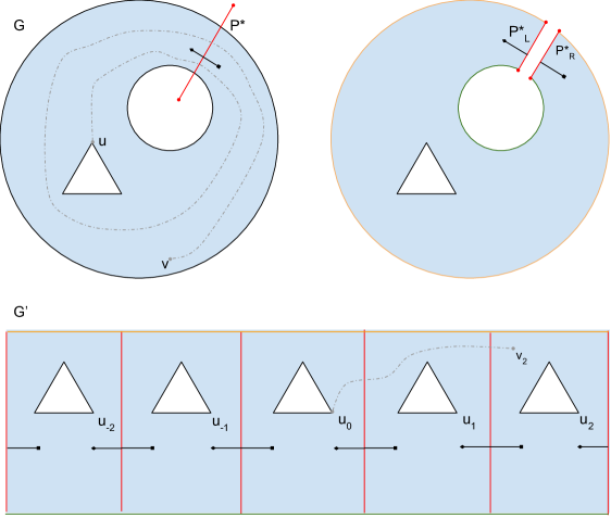
Figure 1: Construction on the graph $G^{\prime}$ from Lemma 6.11. The gray $u\to v$ path in $G$ is preserved in the graph $G^{\prime}$ in the bottom

By construction, every path $R^{\prime}=u_{0}\to v_{j}$ in $G^{\prime}$ corresponds to some path $R=u\to v$ in $G$ with $\pi_{P^{*}}(R)=j$. This implies property $1$.

For a simple path $R=u\to v$ in $G$, $R$ is preserved in $G^{\prime}$ for the following reason. Suppose $R=e_{1}\ldots e_{k}$, where $e_{i}=x_{i}y_{i}$, and denote by $c_{i}$, $i=0,\ldots,k$, the crossing number $\pi_{P^{*}}(\{e_{1},\ldots,e_{i}\})$. That is, the $c_{i}$ is the number of times $e_{1}\ldots e_{i}$ crosses $P^{*}$ left to right, minus the number of times it crosses $P^{*}$ right to left. Note that we have $|c_{i}|\leq i$ and $k\leq n$ since $R$ is simple. As a result, we have $|c_{i}|\leq n$ for all $i$. It follows that a path $R^{\prime}=u_{0}(y_{1})_{c_{1}}(y_{2})_{c_{2}}\ldots(y_{k})_{c_{k}}=u_{0}\to v_{c_{k}}$ exists in $G^{\prime}$ and has the same length as $R$ in $G$. This proves property 2.

Note that all the copies of vertices lying on faces $a$ or $b$ in $G$ lie on a single face of $G^{\prime}$. If some face $f\notin\{a,b\}$ of $G$ is not an intermediate vertex of $P^{*}$, then there are vertex-disjoint copies of $f$ in all parts $\tilde{G}^{\prime}_{i}$ of $G^{\prime}$. This proves property 3. ∎

If $h^{1}_{Q}=h^{2}_{Q}$, then $Q$ is a simple directed cycle in the dual. As discussed earlier, the crossing number $\pi_{u,v}$ of any path $u\to v$ path in $G^{*}_{\lambda}[H](x^{*},y^{*})$ wrt. $Q$ is in $\{-1,0,1\}$ and is uniquely determined by the positions (i.e., exterior or interior) of the vertices $u,v$ wrt. $Q$. As a result, we have $\delta_{G^{*}_{\lambda}[H](x^{*},y^{*})}(u,v)=\delta_{G^{*}_{0}[H](x^{*},y^{*})}(u,v)+\pi_{u,v}\cdot\lambda$. Consequently, the edge weights of $uv$ in $D(H^{*},x^{*},y^{*})$ for $u,v\in V(h)$ can be accessed in $O(1)$ time by shifting the respective weight of $\mathrm{DDG}(G^{*}_{0}[H](x^{*},y^{*}))$ by $\lambda\cdot\pi_{u,v}$. To decompose $\mathrm{DDG}(G^{*}_{\lambda}[H](x^{*},y^{*}))[V(h)]$ into Monge matrices, it is enough to use the decomposition of Lemma 5.2 $O(1)$ times, as follows. Express $V(h)=A\cup B$ so that the sets $A$ and $B$ lie on different sides of $Q$. Then, for each pair $(I,J)\in\{A,B\}^{2}$, we include in the desired decomposition the decomposition of $\mathrm{DDG}(G^{*}_{0}[H](x^{*},y^{*}))$ into Monge matrices but limited to rows $I$ and columns $J$. For each such combination $(I,J)$, the value $\pi_{u,v}$ is equal for all $(u,v)\in I\times J$. Therefore, for each Monge matrix included in our decomposition all its entries get shifted by the same value, which clearly preserves the Monge property. Observe that if $h^{1}_{Q}=h^{2}_{Q}$, this strategy works even for the more involved case of two distinct holes $h^{1}\neq h^{2}$, so we will neglect it later on in Section 6.6.2.

Let us now assume $h^{1}_{Q}\neq h^{2}_{Q}$. Since $h^{1}_{Q}\neq h^{2}_{Q}$, we can build a graph $Z^{\prime}$ from Lemma 6.11 for the graph $G:=Z=G^{*}_{0}[H](x^{*},y^{*})$ and the dual path $P^{*}:=Q$. Using one of the well-known methods, e.g. [EFL18], we enforce uniqueness of shortest paths on the graph $Z^{\prime}$ by only manipulating its edge weights and so that the original path weight can be recovered in $\widetilde{O}(1)$ time from the transformed graph. For any face $f$ of $Z$, denote by $f_{j}$ the face of $Z^{\prime}$ that contains the vertices $\{v_{j}:v\in V(f)\}$, where $v_{j}\in V(Z^{\prime})$ is defined as in Lemma 6.11.

Next, we construct an MSSP data structure on $Z^{\prime}$ with a distinguished face $h_{0}$ (that is, the $0$-th copy of the face $h$ whose vertices‘ pairwise distance are of our interest) in a way that allows accessing the shortest path trees from the vertices on $h_{0}$ via a dynamic tree interface. Note that computing $Z^{\prime}$ and the associated data structures takes $\widetilde{O}(|Z^{\prime}|)=\widetilde{O}(|H|^{2})$ time.

In order to construct the part of $D(H,x^{*},y^{*})$ that is responsible for encoding the distances between the vertices of $V(h)$, we use an auxiliary graph $D_{h}=\left(V(h),\bigcup_{j\in\{-1,0,1\}}E_{h,j}\right)$, satisfying the following. Each $E_{h,j}$ contains for every $u,v\in V(h)$ an edge $uv$ with weight $\delta_{Z^{\prime}}(u_{0},v_{j})+j\cdot\lambda$.

Lemma 6.12.

For any $u,v\in V(h)$, $\delta_{G^{*}_{\lambda}[H](x^{*},y^{*})}(u,v)=\delta_{D_{h}}(u,v)$.

Proof.

Since $G^{*}_{\lambda}[H](x^{*},y^{*})$ has no negative cycles, for any $u,v\in V(h)$, there exists a shortest $u\to v$ path $P$ in $G^{*}_{\lambda}[H](x^{*},y^{*})$ that is simple. As a result, the length of $P$ equals its length in $G^{*}_{0}[H](x^{*},y^{*})$ plus $\lambda\cdot\pi_{Q}(P)$. Recall that the intermediate faces of $Q$ are not holes of $H$. As a result, by Lemma 6.9, $P$ has crossing number $\pi_{Q}(P)$ in $\{-1,0,1\}$. Therefore, the distance from $u$ to $v$ in $D_{h}$ is no more than $\delta_{Z^{\prime}}(u_{0},v_{\pi_{Q}(P)})+\pi_{Q}(P)\cdot\lambda$. By Lemma 6.11, $\delta_{Z^{\prime}}(u_{0},v_{\pi_{Q}(P)})$ is no more than the length of any simple $u\to v$ path in $G^{*}_{0}[H](x^{*},y^{*})$ with crossing number $\pi_{Q}(P)$, in particular, it is no more than the length of $P$ in $G^{*}_{0}[H](x^{*},y^{*})$. Hence, we indeed obtain $\delta_{G^{*}_{\lambda}[H](x^{*},y^{*})}(u,v)\geq\delta_{D_{h}}(u,v)$.

If we had $\delta_{G^{*}_{\lambda}[H](x^{*},y^{*})}(u,v)>\delta_{D_{h}}(u,v)$ for some $u,v\in V(h)$ then there would exist an edge $wz$ in some $E_{h,j}$ with $\delta_{G^{*}_{\lambda}[H](x^{*},y^{*})}(w,z)>\delta_{Z^{\prime}}(w_{0},z_{j})+j\cdot\lambda$. But then there would exist a (not necessarily simple) $w\to z$ path $P\subseteq G^{*}_{0}[H](x^{*},y^{*})$ with $\pi_{Q}(P)=j$ such that its cost in $G^{*}_{\lambda}[H](x^{*},y^{*})$ is less than $\delta_{G^{*}_{\lambda}[H](x^{*},y^{*})}(w,z)$. This is a contradiction in a graph with no negative cycles. ∎

Of course, we cannot build the graph $D_{h}$ explicitly since its size may be $\Theta(|\partial{H}|^{2})$. Note that for any $u,v\in V(h)$, the (minimum) weight of an edge $uv$ in $D_{h}$ can be queried in $\widetilde{O}(1)$ time using the MSSP data structure built on $Z^{\prime}$. However, in order to allow building fast closest pair and near neighbor data structures on $D_{h}$, we still need to efficiently express the edge weights matrix of $D_{h}$ using Monge matrices. Recall that these edge weights encode (shifted) distances between the face $h_{0}$ and faces $h_{-1},h_{0},h_{1}$ in the graph $Z^{\prime}$. The distances between vertices of $h_{0}$ are easily decomposed into Monge matrices with a total of $\widetilde{O}(|V(h_{0})|)$ rows and columns (counted with multiplicity) based on the ordering of vertices on $h_{0}$ exclusively, using the following fact.

Fact 6.13.

Let $A$ and $B$ be two non-interleaving (wrt. to a clockwise order) subsets of vertices lying on a single face of a plane digraph. Let $\mathcal{M}$ be a matrix encoding all-pairs distances from vertices $a\in A$ to vertices $b\in B$. Then, $\mathcal{M}$ is a Monge matrix.

[FR06] apply the above fact a logarithmic number of times to decompose all-pairs distances between $k$ vertices lying on a single face of a plane digraph into Monge matrices with a total of $\widetilde{O}(k)$ rows/columns. These rows/columns depend only on the ordering of the vertices on the face.

The distances between $h_{0}$ and $h_{j}$, if $h_{0}\neq h_{j}$, are more tricky to decompose into an element-wise minimum of Monge matrices. [MW10] deal with this problem by observing that from an arbitrary shortest paths tree $T$ rooted at a vertex $s$ of $h_{0}$, one can choose two paths such that for every two vertices $v_{1},v_{2}$ on the holes $h_{0},h_{j}$ respectively, some shortest $v_{1}\to v_{2}$ path in $Z^{\prime}$ either does not cross the former path or does not cross the latter. Cutting $Z^{\prime}$ along each of these paths (separately) yields two graphs where $V(h_{0})$ and $V(h_{j})$ together lie on a single face (and do not interleave) of the respective graph. As a result, one can view distances between them as a single (full) Monge matrix. The element-wise minimum of distances in the two graphs represents distances between $h_{0}$ and $h_{j}$ in the original graph. Unfortunately, finding the paths used for cutting, actually cutting the graph explicitly, and preprocessing the obtained cut graphs would be too costly in our case.

The following lemma shows a more efficient way to compute the partition of distances between $h_{0}$ and $h_{j}$ into partial Monge matrices, and thus also an efficient construction of closest pair and near neighbor data structures for a graph induced on the edges $E_{h,j}$. Recall that in a partial Monge matrix the elements in each row and each columns are defined only in a consecutive segment of columns or rows, respectively. As a result, for a partial Monge matrix with rows $R$ and columns $C$, it takes only $O(|R|+|C|)$ space to encode which elements are defined: one only needs to encode the ordering of rows and columns, and a single segment in each row. Below, when talking about decomposing into partial Monge matrices, we will mean computing an encoding as defined above.

Lemma 6.14.

Suppose $h_{0}\neq h_{j}$. There exist closest pair and near neighbor data structures for $D_{h}[E_{h,j}]$ with $T_{\mathrm{cp}}(D_{h}[E_{h,j}]),T_{\mathrm{nn}}(D_{h}[E_{h,j}])\in\widetilde{O}(|V(h_{0})|+|V(h_{j})|)$, and $Q_{\mathrm{nn}}(D_{h}[E_{h,j}])=\widetilde{O}(1)$.

Proof.

Recall from Lemma 6.11 that the faces $h_{0}$ and $h_{j}$ in $Z^{\prime}$ are vertex-disjoint. First, pick such $s\in V(h_{0})$ and $t\in V(h_{j})$ that the unique $s\to t$ shortest path $Y$ in $Z^{\prime}$ does not contain any other vertices of $V(h_{0})\cup V(h_{j})$. This can be done in $\widetilde{O}(|V(h_{0})|+|V(h_{j})|)$ time as follows. First pick any $s^{*}\in V(h_{0})$. Then, pick such a $t\in V(h_{j})$ that has the lowest depth in the shortest paths tree from $s^{*}$ stored in the MSSP data structure – this can be done in $\widetilde{O}(|V(h_{j})|)$ time. Finally, on the shortest $s^{*}\to t$ path, pick the deepest vertex $s\in V(h_{0})$ in a similar way. By construction, the $s\to t$ subpath of the $s^{*}\to t$ path contains no other vertices from $V(h_{0})\cup V(h_{j})$.

Fix some vertex $u\in V(h_{0})$. The shortest path $P_{t}=u\to t$ shares some suffix $S$ with $Y$ (possibly only the vertex $t$) due to uniqueness and cannot cross $Y$. Suppose wlog. that $P_{t}$ merges with $Y$ from the left side of $Y$ (the other case is symmetric), and denote by $A$ the set of vertices $u$ with this property (so $u\in A$).

Let us observe that for any $v\in V(h_{j})$, the shortest $u\to v$ path $P_{v}$ does not cross $Y$ right to left: indeed, if the crossing vertex $w$ was at the subpath $S$, this would contradict uniqueness of the $u\to w$ subpath of $P_{t}$. On the other hand, if the path $P_{v}$ crosses $Y$ at vertex $w$ before the subpath $S$, then it would need to cross either $P_{t}\setminus S$ or $Y\setminus S$ once more on the way to $w$, and thus this would violate the uniqueness of $P_{t}$ or $Y$ respectively.

Let us embed an auxiliary vertex $u^{\prime}$ and an edge $u^{\prime}u$ inside the face $h_{0}$ of $Z^{\prime}$ and call that edge the $0$-th sentinel edge of any shortest path $P_{x}=u\to x$. If $x\in V(h_{j})\setminus\{t\}$, then let $e_{x}$ ($e_{x}^{\prime}$) be the earliest edge of the path $P_{x}$ ($P_{t}$, resp.) that does not belong to $P_{t}$ ($P_{x}$, resp.). Note that if $e_{x}$ emerges from the path $P_{t}$ to the left (that is, $e_{x}=ab$ lies between $e_{x}^{\prime}$ and and the preceding edge of $e_{x}^{\prime}$ on $P_{t}$ in the clockwise edge ring of $a$), then $P_{x}$ does not cross $P_{t}$ and thus also does not cross $Y$ (it might still share some prefix with $P_{t}$, and some subpath with $Y$, though). On the other hand, if $e_{x}$ emerges from the path $P_{t}$ to the right, then the shortest $u\to x$ path has to cross $Y$ once. Let $\mathcal{L}_{u}\subseteq V(h_{j})$ contain $t$ and the vertices $x\in V(h_{j})\setminus\{t\}$ such that $e_{x}$ emerges from $P_{t}$ to the left. Similarly, let $\mathcal{R}_{u}\subseteq V(h_{j})$ contain the vertices $x$ of $h_{j}$ such that $e_{x}$ emerges from $P_{t}$ strictly to the right. Since the paths $P_{x}$ for $x\in V(h_{j})$ are pairwise non-crossing, $\mathcal{L}_{u}$ and $\mathcal{R}_{u}$ constitute consecutive fragments of $V(h_{j})$ as ordered on the face $h_{j}$. Moreover, the border between $\mathcal{L}_{u}$ and $\mathcal{R}_{u}$ can be computed via binary search on the vertices $x\in V(h_{j})$: whether $x\in\mathcal{L}_{u}$ or $x\in\mathcal{R}_{u}$ can be decided using an LCA query and a level ancestor query on the shortest path tree from $u$. If we make MSSP use the top tree [AHdLT05] for dynamic tree operations, these queries are supported in polylogarithmic time.

As $Y$ is a unique $s\to t$ shortest path, it is a simple path. Consider a graph $Z^{\prime}_{s,t}$ obtained from $Z^{\prime}$ by cutting $Z$ along the path $Y$ (that is, the vertices and edges of $Y$ appear in $Z^{\prime}_{s,t}$ in two copies). Now, let $Z^{\prime\prime}_{s,t}$ be obtained by gluing two copies of $Z^{\prime}_{s,t}$ along one of the copies of $Y$ (that is, $Z^{\prime\prime}_{s,t}$ contains three copies of $Y$). Denote by $Z^{\prime\prime}_{s,t,L}$ ($Z^{\prime\prime}_{s,t,R}$) the copy of $Z^{\prime}_{s,t}$ to the left (to the right, resp.) of the path $Y$ used for gluing the two copies into $Z^{\prime\prime}_{s,t}$. Note that the graph $Z^{\prime\prime}_{s,t}$ contains two copies of each vertex in $V(h_{0})\setminus\{s\}$ and $V(h_{j})\setminus\{t\}$. For each such vertex $x$, denote by $x_{L},x_{R}$ the copies in the respective parts $Z^{\prime\prime}_{s,t,L}$, $Z^{\prime\prime}_{s,t,R}$. Moreover, $Z^{\prime\prime}_{s,t}$ contains three copies of $s$ and $t$. For $x\in\{s,t\}$, set both $x_{L},x_{R}$ to be the ’’middle‘‘ copy on the copy of path $Y$ used for gluing.

Impose a natural clockwise order starting at $s$ of $V(h_{0})$ on the face $h_{0}$ of $Z^{\prime}$. Similarly, impose a counter-clockwise order on $V(h_{j})$ starting at $t$ on the face $h_{j}$ of $Z^{\prime}$. For $W\subseteq V(Z^{\prime})$, let $W_{L}=\{w_{L}:w\in W\}$ and similarly define $W_{R}$. Note that the vertices $V(h_{0})_{L}$, $V(h_{0})_{R}$, $V(h_{j})_{L}$, $V(h_{j})_{R}$ all lie on a single face $f$ of $Z^{\prime\prime}_{s,t}$ in the clockwise order $V(h_{0})_{L},V(h_{0})_{R},V(h_{j})_{R},V(h_{j})_{L}$, where each of this sets is ordered using the order imposed on the respective original set $V(h_{0})$, $V(h_{j})$.

Observe that every path in $Z^{\prime\prime}_{s,t}$ naturally corresponds to some path in $Z^{\prime}$ (after projecting the copies of vertices to respective original vertices of $Z^{\prime}$). As a result, if some vertices $u^{\prime},v^{\prime}$ of $Z^{\prime\prime}_{s,t}$ are copies of $u,v$ respectively in $Z^{\prime}$, then $\delta_{Z^{\prime\prime}_{s,t}}(u^{\prime},v^{\prime})\geq\delta_{Z^{\prime}}(u,v)$. Moreover, for a shortest path $P_{u,v}=u\to v$ in $Z^{\prime}$, if $u\in A$ and $v\in\mathcal{L}_{u}$, there is a path $u_{L}\to v_{L}$ in $Z^{\prime\prime}_{s,t,L}$ corresponding to $P_{u,v}$. Consequently, $\delta_{Z^{\prime}}(u,v)=\delta_{Z^{\prime\prime}_{s,t}}(u_{L},v_{L})$. Similarly, if $u\in A$ and $v\in\mathcal{R}_{u}$, there is a path $u_{L}\to v_{R}$ in $Z^{\prime\prime}_{s,t}$ corresponding to $P_{u,v}$, and we obtain $\delta_{Z^{\prime}}(u,v)=\delta_{Z^{\prime\prime}_{s,t}}(u_{L},v_{R})$.

Consider a matrix $\mathcal{M}$ with rows $A$ and columns $V(h_{j})_{R}\cup V(h_{j})_{L}$ such that in a row $u\in A$, the elements are defined only for columns $(\mathcal{R}_{u})_{R}\cup(\mathcal{L}_{u})_{L}$. If $k^{\prime}\in(\mathcal{R}_{u})_{R}\cup(\mathcal{L}_{u})_{L}$ is a copy of $k\in V(h_{j})$, then we put $\mathcal{M}_{a,k^{\prime}}=\delta_{Z^{\prime}}(a,k)$. Note that if the columns of $\mathcal{M}$ are ordered as in the clockwise order on the face $f$ of $Z^{\prime\prime}_{s,t}$, then $(\mathcal{R}_{u})_{R}\cup(\mathcal{L}_{u})_{L}$ constitutes a contiguous segment of columns of $\mathcal{M}$.

We now argue that for each column $k^{\prime}$ (such that $k^{\prime}$ is a copy of vertex $k$) of $\mathcal{M}$, the defined elements of that column lie in a consecutive segment of rows of $\mathcal{M}$. Suppose wlog. that $k^{\prime}\in V(h_{j})_{L}$. Then, for $a,b\in A$, the elements $\mathcal{M}_{a,k^{\prime}}$ and $\mathcal{M}_{b,k^{\prime}}$ are both defined iff the shortest paths $P_{a,k}$ and $P_{b,k}$ both do not cross $Y$ in $Z^{\prime}$. Clearly, for any $c\in A$ that lies between $a$ and $b$ in the clockwise order of $V(h_{0})$, the path $P_{c,k}$ is weakly contained in a cycle consisting of $P_{a,k},P_{b,k}$, and the $a\to b$ part of the enclosing cycle of $V(h_{0})$ that does not contain $s$. As a result, since $P_{a,k}$ and $P_{b,k}$ do not cross $Y$, indeed $P_{c,k}$ does not cross $Y$ and we conclude that $\mathcal{M}_{c,k^{\prime}}$ is defined as well.

Since the rows and columns of $\mathcal{M}$ are non-interleaving subsets of vertices on a single face $f$ of $Z_{s,t}^{\prime\prime}$, from Fact 6.13 we conclude that $\mathcal{M}$ is indeed a partial Monge matrix. Note that (values of) the defined elements of $\mathcal{M}$ do not depend on the choice of $s,t$ – they constitute distances in $Z^{\prime}$ and thus can be accessed in $\widetilde{O}(1)$ time using the MSSP data structure that we have built upon $Z^{\prime}$. Any partial $m_{1}\times m_{2}$ Monge matrix can be decomposed into a collection $D$ of full Monge matrices with $\widetilde{O}(m_{1}+m_{2})$ rows and columns (counted with multiplicities). For an intuition and proof, see [GMW20, Lemma 5.1, Theorem 5.5, and Figures 3,4,5].

The defined entries of $\mathcal{M}$ do not quite correspond to the weights of edges $E_{h,j}\cap(A\times V(h_{j}))$: the columns of $\mathcal{M}$ include two copies of each vertex of $V(h_{j})$. However, we can easily obtain a graph $G_{h,j}$ whose $A\times V(h_{j})$ distances are equal to the weights of $E_{h,j}\cap(A\times V(h_{j}))$. Let the vertices of $G_{h,j}$ be $A\cup V(h_{j})_{L}\cup V(h_{j})_{R}\cup V(h_{j})$. $G_{h,j}$ contains a subgraph $G_{\mathcal{M}}$ with edges between $A$ and $V(h_{j})_{L}\cup V(h_{j})_{R}$ corresponding to the defined elements of $\mathcal{M}$, and $2|V(h_{j})|$ auxiliary edges $u_{L}u,u_{R}u$ of weight $0$ for all $u\in V(h_{j})$. Similarly as in the proof of Lemma 5.1, we can use the data structure of [MNW18, Lemma 1] and the Monge heap to obtain (via Lemmas 3.5 and 3.2 applied to the decomposition $D$ of $\mathcal{M}$ into full Monge matrices) near neighbor and closest pair data structures for $G_{\mathcal{M}}$ with total update time $\widetilde{O}(|V(h_{0})|+|V(h_{j})|)$ and query time $\widetilde{O}(1)$. To obtain the desired closest pair and near neighbor data structures for $G_{h,j}$ (which, as argued above, can serve as the respective data structures for $D_{h}[E_{h,j}]$) we simply apply Lemmas 3.2 and 3.5 once again to the data structures for $G_{\mathcal{M}}$ and the trivial data structures for $G_{h,j}\setminus G_{\mathcal{M}}$ which contain $\widetilde{O}(|V(h_{0})|+|V(h_{j})|)$ auxiliary non-structured edges.

We proceed symmetrically with the distances from $V\setminus A$ to $V(h_{j})$. Finally, we merge the obtained data structure for graphs representing distances $A\times V(h_{j})$ and $(V\setminus A)\times V(h_{j})$, resp. into a single one with asymptotically same time bounds using Lemmas 3.2 and 3.5. ∎

With the data structures of Lemma 6.14 in hand, we can again apply Lemmas 3.5 and 3.2 to get the desired data structures for $D_{h}=D_{h}[E_{h,-1}]\cup D_{h}[E_{h,0}]\cup D_{h}[E_{h,1}]$ with total update time $\widetilde{O}\left(|V(h)|\right)=\widetilde{O}(|\partial{H}|)$ and query time $\widetilde{O}(1)$. This way, we achieve our goal for the case $h^{1}=h^{2}$.

6.6.2 The case of two distinct holes

The primary difference between the case $h^{1}\neq h^{2}$ and the single-hole case is that it is no longer the case that the crossing number of a path from $h^{1}$ to $h^{2}$ has wrt. $Q$ is necessarily in $\{-1,0,1\}$. We will nevertheless prove the following. Recall that we have already handled the case $h^{1}_{Q}=h^{2}_{Q}$, so below we assume $h^{1}_{Q}\neq h^{2}_{Q}$.

Lemma 6.15.

Let $s\in V(h^{1})$, $t\in V(h^{2})$, where $h^{1}\neq h^{2}$. Suppose there exists a simple shortest ${s\to t}$ path $P$ in $G^{*}_{\lambda}[H](x^{*},y^{*})$ such that $V(P)\cap(V(h^{1})\cup V(h^{2}))=\{s,t\}$ with crossing number $\pi_{Q}(P)$. Then, for any $(u,v)\in V(h^{1})\times V(h^{2})$, there exists some shortest $u\to v$ path in $G^{*}_{\lambda}[H](x^{*},y^{*})$ with crossing number wrt. $Q$ in $[\pi_{Q}(P)-4,\pi_{Q}(P)+4]$.

Proof.

Since $P$ is a shortest path that is simple, there exists some simple shortest path $S=u\to v$ that does not cross $P$ more than once (either from left to right or right to left). Let us focus on the case when $P$ and $S$ have at least one vertex in common, and $S$ indeed crosses $P$ once, wlog. left to right. The other cases, when $P$ and $S$ are completely disjoint or when they have a common part, but do not cross, are easier to handle, and can by considered analogously.

Since $P$ and $S$ have a vertex in common, one can write $P=P_{1}RP_{2}$, $S=S_{1}RS_{2}$, where $x\to y=R\subseteq P$ is a possibly empty (i.e., containing zero edges) maximal common subpath of $P$ and $S$, and $S_{1},S_{2}$ can share only endpoints with $V(P)$.

Let $G^{+}$ be the graph obtained from $G^{*}_{\lambda}[H](x^{*},y^{*})$ by cutting it along $P$, so that $G^{+}$ has two copies of the vertices and edges of $P$. Denote by $P_{L},P_{R}$ the left and right copies of $P$ respectively, and by $w_{L},w_{R}$ the respective left and right copies of a vertex $w\in V(P)$. For all $w\in V(H)\setminus V(P)$, set $w_{L}=w_{R}=v$. In this graph, the vertices $(V(h^{1})\setminus\{s\})\cup(V(h^{2})\setminus\{t\})$ lie on a single face $f$, and each of the two sets comprising this union forms a segment of consecutive vertices on $f$. The other vertices on $f$ come from the two copies of $P$. These sets also form contiguous segments on $f$, and one can easily see that the ordering of vertices on $f$ can be wlog. assumed to be $V(h^{1}),V(P_{L}),V(h^{2}),V(P_{R})$, where $V(P_{L})$ starts with $s_{L}$, and $V(P_{R})$ starts with $t_{R}$.

Note that for $S_{1}=u\to x$, there exists a unique corresponding path $S_{1}^{+}=u_{L}\to x_{L}$ in $G^{+}$. Similarly, for $S_{2}=y\to v$, there exists a unique corresponding path $S_{2}^{+}=y_{R}\to v_{R}$ in $G^{+}$. Let $P_{1}^{+}$ be the $s_{L}\to x_{L}$ subpath of $P_{L}$, and let $P_{2}^{+}$ be the $y_{R}\to t_{R}$ subpath of $P_{R}$ in $G^{+}$.

Consider the effect that cutting along $P$ has on the dual path $Q$. Express $Q$ as$Q_{1}\cdot e_{1}\cdot Q_{2}\cdot e_{2}\cdot\ldots\cdot e_{k-1}\cdot Q_{k}$ such that $P$ and $Q$ cross at edges $e_{1},\ldots,e_{k-1}$. Let $i\in\{2,\ldots,k-1\}$. In $G^{+}$, each subpath $e_{i-1}\cdot Q_{i}\cdot e_{i}$ of $Q$ corresponds to a simple curve $Q_{i}^{+}$ with both its endpoints inside the face $f$, and intersecting the bounding cycle of $f$ at copies of edges $e_{i-1},e_{i}$. As a result, each such $Q_{i}^{+}$ crosses $f$ at some two points of $f$ that lie on the segments spanned by either $V(P_{L})$ or $V(P_{R})$ on $f$. See Figure 2 for better understanding. Regardless of which segments $Q_{i}^{+}$ crosses, every path from $V(h^{1})\setminus\{s\}\cup\{s_{L}\}$ to some other fixed vertex $w$ on $f$ in $G^{+}$ has the same crossing number wrt. $Q_{i}^{+}$ because $V(h^{1})$ lies entirely on one side of the dual cycle $Q_{i}^{+}\subseteq G^{+}$. For an analogous reason, every path from some fixed vertex $w$ on $f$ to a vertex of $V(h^{2})\setminus\{t\}\cup\{t_{R}\}$ has the same crossing number wrt. $Q_{i}^{+}$. So the crossing numbers of $P_{j}^{+}$ and $S_{j}^{+}$ (for $j=1,2$) wrt. $Q_{i}^{+}$ are equal.

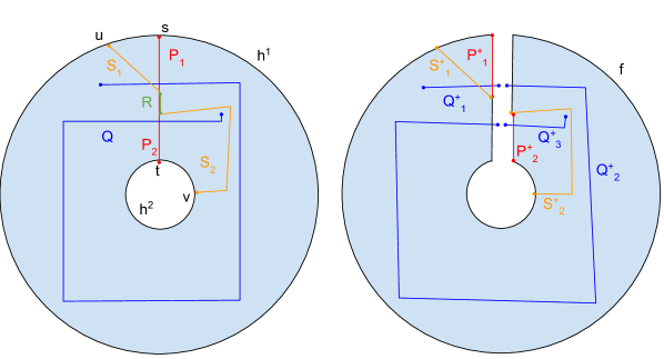
Figure 2: Illustration for the proof of Lemma 6.15.

On the other hand, observe that the crossing number of $P_{j}$ wrt. $Q$, for $j=1,2$, equals the sum of crossing numbers of $P_{j}^{+}$ wrt. $Q_{2}^{+},\ldots,Q_{k-1}^{+}$. This is because the crossing number of $P_{j}$ wrt. each $Q_{l}$, where $l=1,\ldots,k$ is $0$ (by the definition of $Q_{l}$), and the crossing number of $P_{j}$ wrt. some $e_{l}$, where $l=1,\ldots,k-1$, contributes to precisely one of the crossing numbers of $P_{j}^{+}$ wrt. $Q^{+}_{i}$. Moreover, the crossing number of $S_{j}$ wrt. $e_{1}\cdot Q_{2}\cdot e_{2}\cdot\ldots\cdot Q_{k-1}\cdot e_{k-1}$, equals the sum of crossing numbers of $S_{j}^{+}$ wrt. $Q_{2}^{+},\ldots,Q_{k-1}^{+}$. To see this, recall that $S_{j}$, disjoint with $P$, has crossing number $0$ with all $e_{l}$. But we have proved that the crossing numbers of $P_{j}^{+}$ and $S_{j}^{+}$ wrt. each $Q_{i}^{+}$ are equal, and thus we conclude that the crossing number of $P_{j}$ wrt. $Q$ equals the crossing number of $S_{j}$ wrt. $Q\setminus Q_{1}\setminus Q_{k}$.

We now argue that the crossing number of $S_{j}$ wrt. $Q_{1}$ or $Q_{k}$ is in $\{-1,0,1\}$. It will follow that the crossing number of $P_{j}$ wrt. $Q$ can deviate by at most $2$ from the crossing number of $S_{j}$ wrt. $Q$. Let us focus on the crossing number wrt. $Q_{1}$, as the other case is analogous. Since $Q_{1}$ is preserved in $G^{+}$, and $S_{j}$ is preserved in $G^{+}$ as $S_{j}^{+}$, the crossing number of $S_{j}$ wrt. $Q_{1}$ in $G^{*}_{\lambda}[H](x^{*},y^{*})$ equals the crossing number of $S_{j}^{+}$ wrt. $Q_{1}$ in $G^{+}$. But the endpoints of the simple path $S_{j}^{+}$ lie on a single face $f$ of $G^{+}$, and no intermediate vertex of $Q_{j}$ (seen as a dual path in $G^{+}$) equals $f$, so the crossing number of $Q_{j}$ wrt. $S_{j}^{+}$ is in $\{-1,0,1\}$ by Lemma 6.9.

To summarize, the crossing numbers of $P_{j}$ and $S_{j}$ wrt. $Q$ may differ by at most $2$. We conclude that the crossing numbers of $P=P_{1}RP_{2}$ and $S=S_{1}RS_{2}$ wrt. $Q$ can differ by at most $4$. ∎

Lemma 6.16.

Let the holes $h^{1},h^{2}$, where $h^{1}\neq h^{2}$, be fixed. In $\widetilde{O}(|H|^{2})$ time one can build a data structure answering queries of the following form in $\widetilde{O}(1)$ time. Given $\lambda\in[0,\lambda^{*}]$, find some two vertices $s\in V(h^{1})$, $t\in V(h^{2})$ and a number $k$ such that there exists a simple shortest $s\to t$ path $P$ in $G^{*}_{\lambda}[H](x^{*},y^{*})$ with $V(P)\cap(V(h^{1})\cup V(h^{2}))=\{s,t\}$ and the crossing number of $P$ wrt. $Q$ is $k$.

Proof.

Consider the graph $Z^{\prime}$ (built using Lemma 6.11) from Section 6.6.1. Recall that for each vertex $v$ of $G^{*}_{0}[H](x^{*},y^{*})$, $Z^{\prime}$ has $2n+1$ copies $v_{-n},\ldots,v_{n}$ of $v$ so that a path from any $u_{0}$ to $v_{j}$ corresponds to an $u\to v$ path in $G^{*}_{0}[H](x^{*},y^{*})$ with crossing number $j$ wrt. $Q$.

Pick any $s^{\prime}\in V(h^{1})$ and $t^{\prime}\in V(h^{2})$. Compute a shortest paths tree $T$ from $s^{\prime}_{0}$ in $Z^{\prime}$. This takes $O(|Z^{\prime}|)=O(|H|^{2})$ time. Denote by $T[v_{j}]$ the $s^{\prime}_{0}\to v_{j}$ path in that tree, and by $\ell(T[v_{j}])$ its length.

Similarly as in Lemma 6.11, one can prove that $T[t^{\prime}_{j}]$ corresponds to some $s^{\prime}\to t^{\prime}$ path in $G^{*}_{0}[H](x^{*},y^{*})$ with crossing number wrt. $Q$ exactly $j$ and not longer than the shortest simple $s^{\prime}\to t^{\prime}$ path in that graph with crossing number $j$. Consequently, by proceeding as in the proof of Lemma 6.12, we obtain that the length of the shortest $s^{\prime}\to t^{\prime}$ path in $G^{*}_{\lambda}[H](x^{*},y^{*})$ equals

$$\min_{j\in\{-n,\ldots,n\}}\{\ell(T[t^{\prime}_{j}])+\lambda\cdot j\},$$

and if some $j$ minimizes the above for a given $\lambda$, then the path $T[t_{j}^{\prime}]$ can be projected to an $s^{\prime}\to t^{\prime}$ path in $G^{*}_{\lambda}[H](x^{*},y^{*})$ with cost precisely $\ell(T[t^{\prime}_{j}])+\lambda\cdot j$, that is, a shortest $s^{\prime}\to t^{\prime}$ path.

In order to be able to compute a minimizer $j$ given some $\lambda$, we apply the following preprocessing. We want to compute a minimum of $2n+1=O(|H|)$ linear functions at coordinate $\lambda$. It is well-known that such a minimum is the lower envelope of these functions and can be described using $k\leq 2n$ breakpoints $\lambda_{1},\ldots,\lambda_{k}$ and numbers $j_{1},\ldots,j_{k}$, $j_{1}\geq\ldots\geq j_{k}$, such that for every $i=0,\ldots,k$, the minimum at $\lambda\in[\lambda_{i},\lambda_{i+1})$ equals $\ell(T[t^{\prime}_{j_{i}}])+\lambda\cdot j_{i}$ (where $\lambda_{0}=-\infty$ and $\lambda_{k+1}=\infty$). The lower envelope can be easily computed in linear time. With the breakpoints, locating the path $T[t^{\prime}_{j^{*}}]$ that achieves the minimum for a given $\lambda$ can be done using binary search in $\widetilde{O}(1)$ time.

The last problem is that the projection of $T[t^{\prime}_{j^{*}}]$ might not correspond to a simple path in $G^{*}_{\lambda}[H](x^{*},y^{*})$, and it may contain more than two vertices of $V(h^{1})\cup V(h^{2})$. To deal with this problem, we make another preprocessing step on the tree $T$ so that to any $T[v_{j}]$ with $v\in V(h^{2})$ we assign a simple path $P^{*}_{v_{j}}\subseteq G^{*}_{0}[H](x^{*},y^{*})$ from $V(h^{1})$ to $V(h^{2})$ such that $P^{*}_{v_{j}}$ is a projection of a subpath of $T[v_{j}]\subseteq Z^{\prime}$ onto $G^{*}_{0}[H](x^{*},y^{*})$. Note that if (the projection of) $T[t^{\prime}_{j^{*}}]$ is a shortest $s^{\prime}\to t^{\prime}$ path in $G^{*}_{\lambda}[H](x^{*},y^{*})$, then $P^{*}_{t^{\prime}_{j^{*}}}$, being a projection of a subpath of $T[t^{\prime}_{j^{*}}]$, is also a shortest path in $G^{*}_{\lambda}[H](x^{*},y^{*})$ that meets the desired requirements. Recall that we are only asked to return the endpoints of such a path, and its crossing number wrt. $Q$.

We process the vertices $T$ in pre-order. On the way, we maintain a data structure $\mathcal{D}$. We maintain the following invariant: before the processing of $v_{j}$ (whose parent is $p_{l}$) starts, and also after it finishes, $\mathcal{D}$ stores some simple $s^{\prime}\to p$ path $P_{p}$ in $G^{*}_{0}[H](x^{*},y^{*})$ that is a projection of a subpath of $T[p_{l}]$. We will first describe how the data structure is used, and explain how its operations are implemented later.

Let $e_{v_{j}}$ be the parent edge of $v_{j}$ in $T$, and let $e_{v}$ be the corresponding edge in $G^{*}_{0}[H](x^{*},y^{*})$. To process the vertex $v_{j}$, we first check whether the path $P_{p}$ contains $v$. Since $P_{p}$ is simple, it might contain at most one occurrence of $v$. Suppose $P_{p}=R_{1}R_{2}$, where $R_{1}=s^{\prime}\to v$. In this case, the path $R_{1}$ forms a simple $s^{\prime}\to v$ path $P_{v}$ that is a projection of a subpath of $T[p_{l}]$, so we may set $P_{v}:=R_{1}$. On the other hand, if $P_{p}$ does not contain $v$, we may simply set $P_{v}:=P_{p}\cdot e_{v}$ and achieve the same. We update the data structure $\mathcal{D}$ so that it stores $P_{v}$. If $v\in V(h^{2})$, we use $\mathcal{D}$ to find the first vertex $t_{v}\in V(h^{2})$ on $P_{v}$ (if exists), and then the latest vertex $s_{v}\in V(h^{1})$ on $P_{v}$ that precedes the occurrence $t_{v}$. Note that the $s_{v}\to t_{v}$ subpath of $P_{v}$ is simple, does not contain any other vertices of $V(h^{1})\cup V(h^{2})$ apart from the endpoints $s_{v},t_{v}$, and is a projection of a subpath of $T[v_{j}]$. We thus let $P^{*}_{v_{j}}$ equal that $s_{v}\to t_{v}$ subpath of $P_{v}$. We then record the endpoints $s_{v},t_{v}$ of $P^{*}_{v_{j}}$ and its crossing number wrt. $Q$. Afterwards, we process the children of $v$ recursively. Note that the invariant posed on $\mathcal{D}$ is met. When all the children of $v$ are processed, we revert changes to $\mathcal{D}$ so that it again stores $P_{p}$ instead of $P_{v}$.

We now explain how to implement the data structure $\mathcal{D}$ storing a simple path $P$ in $G^{*}_{0}[H](x^{*},y^{*})$. First of all, $\mathcal{D}$ stores two arrays $A,I$, and the number of edges $q$ of the stored path $P$. The array $A$ stores the subsequent vertices of $P$ at positions $1,\ldots,q$. $I$ is indexed with vertices of $H$: the vertex $v$ might appear on $P$ only at position $I[v]$ (if such a position exists). It might still hold that $A[I[v]]\neq v$; then $P$ does not contain the vertex $v$.

Moreover, we store the positions of vertices from $V(h^{1})$ on the path $P$ in an array $L$. More precisely, if the vertices of $V(h^{1})$ appear on positions $l_{1},\ldots,l_{g}$ on $P$, then $L[i]=l_{i}$ for all $i=1,\ldots,g$. We also maintain the first occurrence of a vertex from $V(h^{2})$ on the path $P$.

Finally, we also store the crossing numbers of all prefixes of $P$ in an array $S$. That is, if $i\leq q$, then $S[i]$ is the crossing number of the subpath $s^{\prime}\to A[i]$ of $P$. Storing prefix crossing numbers allows us to compute the crossing number of any subpath of $P$ in $O(1)$ time by subtracting two crossing numbers of path prefixes.

Suppose once again we start processing a vertex $v_{j}$ with parent $p_{l}$. The array $I$ can locate the occurrence of $v$ on $P_{p}$, if it exists. To make $\mathcal{D}$ store $P_{v}$, we either simply decrease $q$ (to $I[v]$) if $P_{p}$ contains $v$ or increase $q$ by one and update $A[q]$, $S[q],I[v]$ in $O(1)$ time. If $v\in V(h^{1})$, we also update $L$ if no occurrence of $v$ has been found in $P_{p}$, as follows. We find the first $L[i]$ with $L[i]\geq\ell$ (via binary search) and set $L[i]:=v$. Updating the first occurrence of a vertex from $V(h^{2})$ is trivial. It is easy to check that this update process is correct and all the invariants are satisfied. Moreover, it takes $O(\log{n})$ time, and involves updating $O(1)$ values in the worst case. As a result, after descending down the tree recursively, we can efficiently revert all the updates to $\mathcal{D}$ in $O(1)$ time so that after the processing of a vertex $v_{j}$ ends, $\mathcal{D}$ stores $P_{p}$ again.

To find the subpath $s_{v}\to t_{v}$ of $P_{v}$, it is enough to binary search for the latest position in $L$ that is smaller than $I[t_{v}]$. Note that this only happens if $v\in V(h^{2})$, so $t_{v}$ is well-defined here, and the requested position can be found since $L[1]=1$. The crossing number of the $P^{*}_{v_{j}}=s_{v}\to t_{v}$ can be read from the array $S$.

We conclude that finding the required endpoints and crossing numbers of $P_{v_{j}}^{*}$ for all $v_{j}$ can be done using additional $\widetilde{O}(|T|)=\widetilde{O}(|Z^{\prime}|)=\widetilde{O}(|H|^{2})$ preprocessing time, as desired. ∎

Equipped with Lemmas 6.15 and 6.16, obtaining the closest pair and near neighbor data structures for the subgraph of $D(H,x^{*},y^{*})$ encoding the distance between $V(h^{1})$ and $V(h^{2})$ is relatively easy. First, during preprocessing, we compute the data structure of Lemma 6.16. Given some $\lambda$, in $\widetilde{O}(1)$ time we can find such $s\in V(h^{1})$, $t\in V(h^{2})$ that some simple shortest $s\to t$ path $P$ in $G^{*}_{\lambda}[H](x^{*},y^{*})$ has crossing number $k$, and $V(P)\cap(V(h^{1})\cup V(h^{2}))=\{s,t\}$. By Lemma 6.15, for every $(u^{\prime},v^{\prime})\in V(h^{1})\times V(h^{2})$, some shortest $u^{\prime}\to v^{\prime}$ path in $G^{*}_{\lambda}[H](x^{*},y^{*})$ has crossing number between $k-4$ and $k+4$.

Similarly as in Section 6.6.1, we consider an auxiliary graph

$$D_{h^{1},h^{2}}=\left(V(h^{1})\cup V(h^{2}),\bigcup_{j\in[k-4,k+4]}E_{h^{1},h^{2},j}\right),$$

where each $E_{h^{1},h^{2},j}$ contains, for each $(u,v)\in V(h^{1})\times V(h^{2})$, an edge $uv$ with weight $\delta_{Z^{\prime}}(u_{0},v_{j})+j\cdot\lambda$.

Analogously as in Lemma 6.12, from the definition of $k$, one can prove that for all ${(u,v)\in V(h^{1})\times V(h^{2})}$, $\delta_{G^{*}_{\lambda}[H](x^{*},y^{*})}(u,v)=\delta_{D_{h^{1},h^{2}}}(u,v)$. Finally, observe that the proof of Lemma 6.14 is valid not only for the graphs $D_{h}[E_{h,j}]$ from Section 6.6.1, but also for each of the graphs $D_{h^{1},h^{2}}[E_{h^{1},h^{2},j}]$. Indeed, there, the goal was to decompose distances between the distinct faces $h_{0}$ and $h_{j}$ of $Z^{\prime}$. The proof goes through without any changes if we replace $h_{0}$ with $h^{1}_{0}$, and $h_{j}$ with $h^{2}_{j}$. Consequently, we obtain data structures with $T_{\mathrm{cp}}(D_{h^{1},h^{2}}[E_{h^{1},h^{2},j}]),T_{\mathrm{nn}}(D_{h^{1},h^{2}}[E_{h^{1},h^{2},j}])\in\widetilde{O}(|V(h^{1})|+|V(h^{2})|)=\widetilde{O}(|\partial{H}|)$, and $Q_{\mathrm{nn}}(D_{h^{1},h^{2}}[E_{h^{1},h^{2},j}])=\widetilde{O}(1)$. By combining those for $O(1)$ required values $j\in[k-4,k+4]$ as previously, we obtain that $T_{\mathrm{cp}}(D_{h^{1},h^{2}}),T_{\mathrm{nn}}(D_{h^{1},h^{2}})\in\widetilde{O}(|V(h^{1})|+|V(h^{2})|)=\widetilde{O}(|\partial{H}|)$, and $Q_{\mathrm{nn}}(D_{h^{1},h^{2}})=\widetilde{O}(1)$. This concludes the proof of Lemma 6.8.

7 Flows, circulations, and negative cycle detection

Let $G_{0}=(V,E_{0})$ be the input directed graph. Let $n=|V|$ and $m=|E_{0}|$. Define $G=(V,E)$ to be a flow network, i.e., a multigraph such that $E=E_{0}\cup E_{0}^{\mathrm{R}}$, $E_{0}\cap E_{0}^{\mathrm{R}}=\emptyset$, where $E_{0}^{\mathrm{R}}$ is the set of reverse edges. For any $uv=e\in E$, there is an edge $e^{\mathrm{R}}\in E$ such that $e^{\mathrm{R}}=vu$ and $(e^{\mathrm{R}})^{\mathrm{R}}=e$. We have $e\in E_{0}$ iff $e^{\mathrm{R}}\in E_{0}^{\mathrm{R}}$.

Let $u:E_{0}\to\mathbb{Z}_{+}\cup\{\infty\}$ be an integral capacity function. A flow is a function $f:E\to\mathbb{R}$ such that for any $e\in E$ $f(e)=-f(e^{\mathrm{R}})$ and for each $e\in E_{0}$, $0\leq f(e)\leq u(e)$. These conditions imply that for $e\in E_{0}$, $-u(e)\leq f(e^{\mathrm{R}})\leq 0$. We extend the function $u$ to $E$ by setting $u(e^{\mathrm{R}})=0$ for all $e\in E_{0}$. Then, for all edges $e\in E$ we have $-u(e^{\mathrm{R}})\leq f(e)\leq u(e)$.

The excess $\mathrm{exc}_{f}(v)$ of a vertex $v\in V$ is defined as $\sum_{uv=e\in E}f(e)$. Due to anti-symmetry of $f$, $\mathrm{exc}_{f}(v)$ is equal to the amount of flow going into $v$ by the edges of $E_{0}$ minus the amount of flow going out of $v$ by the edges of $E_{0}$. The vertex $v\in V$ is called an excess vertex if $\mathrm{exc}_{f}(v)>0$ and a deficit vertex if $\mathrm{exc}_{f}(v)<0$. Let $X$ be the set of excess vertices of $G$ and let $D$ be the set of deficit vertices. Define the total excess $\Psi_{f}$ as the sum of excesses of the excess vertices, i.e., $\Psi_{f}=\sum_{v\in X}\mathrm{exc}_{f}(v)=\sum_{v\in D}-\mathrm{exc}_{f}(v).$

A flow $f$ is called a circulation if there are no excess vertices, or equivalently, $\Psi_{f}=0$.

Let $c:E_{0}\to\mathbb{R}$ be the input cost function. We extend $c$ to $E$ by setting $c(e^{\mathrm{R}})=-c(e)$ for all $e\in E_{0}$. The cost $c(f)$ of a flow $f$ is defined as $\frac{1}{2}\sum_{e\in E}f(e)c(e)=\sum_{e\in E_{0}}f(e)c(e)$.

To send a unit of flow through $e\in E$ means to increase $f(e)$ by $1$ and simultaneously decrease $f(e^{\mathrm{R}})$ by $1$. By sending a unit of flow through $e$ we increase the cost of flow by $c(e)$. To send a unit of flow through a path $P$ means to send a unit of flow through each edge of $P$. In this case we also say that we augment flow $f$ along path $P$.

The residual network $G_{f}$ of $f$ is defined as $(V,E_{f})$, where $E_{f}=\{e\in E:f(e)<u(e)\}$. The capacity of an edge $e\in E_{f}$ in the residual network $G_{f}$ is defined as $u(e)-f(e)$.

For any $v\in V$, let us define:

$$\lambda_{v}=\min\left(\sum_{uv=e\in E}u(e),\sum_{vw=e\in E}u(e)\right).$$

For example, if $G$ is a unit-capacitated network, then $\lambda_{v}$ equals the minimum of the indegree and the outdegree of $v$ in the underlying network $G_{0}$. Let us also put

$$\Lambda:=\sum_{v\in V}\lambda_{v}.$$

In the following we will assume that $\Lambda\geq n$, as vertices with $\lambda_{v}=0$ are of no use in the minimum-cost circulation problem.

Moreover, we will assume that $\Lambda$ is finite. Observe that finite $\Lambda$ implies that any circulation has finite flow values. As a result, the cost of a minimum-cost circulation is finite as well.

Let us partition $E_{0}$ into $E_{\mathrm{fin}}\cup E_{\infty}$ so that for all $e\in E_{\infty}$, $u(e)=\infty$, and $E_{\mathrm{fin}}=E_{0}\setminus E_{\infty}$. Let us put $G_{\infty}:=G\setminus E_{\mathrm{fin}}$ and $m_{\mathrm{fin}}=|E_{\mathrm{fin}}|$. Let $C=\max(2,\max\{-c(e):e\in E_{0}\})$.

In Section 8 we prove:

Theorem 7.1.

Suppose closest pair and near neighbor data structures have been preprocessed for $G_{\infty}$. Let $f^{*}$ be a min-cost circulation in $G$. Then, an integral circulation $f_{\delta}$ satisfying

$$c(f^{*})\leq c(f_{\delta})\leq c(f^{*})+\delta$$

can be computed in time:

$$\widetilde{O}\left(\sqrt{\Lambda}\log{(\Lambda C/\delta)}\cdot\left(T_{\mathrm{cp}}(G_{\infty})+T_{\mathrm{nn}}(G_{\infty})+m_{\mathrm{fin}}+\Lambda\cdot Q_{\mathrm{nn}}(G_{\infty})\right)\right).$$

Within the same bounds, a price function $\pi$ satisfying $c_{\pi}(e)\geq-\delta/\Lambda$ for all $e\in E(G_{f_{\delta}})$ is produced.

Before proving Theorem 7.1, let us deduce Theorem 3.6 from it. See 3.6

Proof.

We use a reduction similar to that of [Gab85, GT89]. Consider a flow network $G^{\prime}$ obtained from $G$ by converting weights to costs, setting all capacities to $\infty$, vertex splitting, and subsequently adding, for each $u\in V$, an edge $u_{\textrm{in}}u_{\textrm{out}}$ of capacity $1$ and cost $0$. Note that for $G^{\prime}$, $\Lambda=n$ holds.

Observe that the subgraph of infinite-capacity edges $G_{\infty}$ of $G^{\prime}$ satisfies $T_{\mathrm{cp}}(G_{\infty})=\widetilde{O}(T_{\mathrm{cp}}(G))$ by Lemma 4.6. Moreover, we have $T_{\mathrm{nn}}(G_{\infty})=O(T_{\mathrm{nn}}(G))$ and $Q_{\mathrm{nn}}(G_{\infty})=O(Q_{\mathrm{nn}}(G))$ by Observation 4.5.

Clearly, $G$ has a negative cycle if and only if $G^{\prime}$ has a negative cycle. Let us now argue that $G^{\prime}$ has a negative cycle if and only if the minimum-cost circulation $f^{*}$ in $G^{\prime}$ has negative cost. Observe that a zero circulation (i.e., where the flow on each edge is $0$) is a valid circulation of cost $0$. As a result, we have $c(f^{*})\leq 0$.

Suppose $G^{\prime}$ has a negative cycle. Then, by sending a unit of flow through that cycle, we obtain a valid circulation of negative cost, i.e., we conclude $c(f^{*})<0$.

Now suppose that $c(f^{*})<0$. It is well-known (see e.g. [AMO93]) that any circulation – in particular $f^{*}$ – can be decomposed into cycles in $G^{\prime}$ of positive flow. Since the sum of costs of these cycles is negative, at least one of them has to have a negative cost.

Since the costs and capacities are integral or infinite, and $\Lambda$ is finite for $G^{\prime}$, $c(f^{*})$ is integral. As a result, $c(f^{*})<0$ implies $c(f^{*})\leq-1$. Hence, if we invoke Theorem 7.1 to compute an integer circulation $f_{\delta}$ with $\delta\leq\frac{1}{2}$, to be set later, then $c(f_{\delta})\leq-1+\delta\leq-\frac{1}{2}<0$. We conclude that $c(f^{*})<0$ implies $c(f_{\delta})<0$. Since $f^{*}$ is an optimal circulation, $c(f_{\delta})<0$ trivially implies $c(f^{*})<0$. As a result, $G$ has a negative cycle iff $c(f_{\delta})<0$. For the graph $G^{\prime}$ we have $\Lambda=n$, and $G^{\prime}$ has $O(n)$ finite-capacity edges, so computing $f_{\delta}$ takes

$$\widetilde{O}\left(\sqrt{n}\cdot(T_{\mathrm{cp}}(G_{\infty})+T_{\mathrm{nn}}(G_{\infty})+n\cdot Q_{\mathrm{nn}}(G_{\infty}))\cdot\log(C/\delta)\right)$$

time by Theorem 7.1. Note that if one decomposes the circulation $f_{\delta}$ into cycles of positive flow, at least one of them will be negative. Such a cycle in $G^{\prime}$ can be easily converted to a simple negative cycle in $G$.

However, if $c(f^{*})=0$, i.e., $G$ has no negative cycle, we still need to produce a feasible price function of $G$. To this end we need the feasible price function $\pi$ produced by Theorem 7.1 when computing $f_{\delta}$. Note that $c(f_{\delta})\leq\delta\leq\frac{1}{2}$ implies $c(f_{\delta})=0$ by integrality of $f_{\delta}$.

Since $f_{\delta}$ is a circulation, it can be decomposed into a collection of $j\geq 0$ simple cycles $C_{1},\ldots,C_{j}$, of positive flow (in fact, a unit flow). In fact, each of these cycles has to have $0$ cost, as otherwise at least one of them would have negative cost. Consider one of the cycles $C_{i}$. Since $C_{i}$ is a simple cycle, it has at most $2n$ edges (recall that vertex splitting doubles the number of vertices). Consider any edge $uv\in C_{i}$. Clearly, since $f_{\delta}(uv)=1$, $vu\in G^{\prime}_{f_{\delta}}$ and thus

$$-c(uv)-\pi(v)+\pi(u)=c(vu)-\pi(v)+\pi(u)=c_{\pi}(vu)\geq-\frac{\delta}{n}$$

by Theorem 7.1. Equivalently, $c(uv)-\pi(u)+\pi(v)\leq\frac{\delta}{n}$. Suppose we have $c(xy)-\pi(x)+\pi(y)<-2\delta$ for some edge $xy\in C_{i}$. Then the sum

$$\sum_{uv\in C_{i}}(c(uv)-\pi(u)+\pi(v))$$

has terms no more than $\frac{\delta}{n}$, and at least one term less than $-2\delta$, so it is less than ${\frac{(2n-1)\delta}{n}-2\delta<0}$. But since $C_{i}$ is a cycle, the prices $\pi(\cdot)$ in the above sum cancel out, so we actually obtain $\sum_{uv\in C_{i}}c(uv)<0$ which contradicts that $C_{i}$ has zero cost. Therefore, we conclude that for any edge $uv\in C_{i}$ we have:

$$c(uv)-\pi(u)+\pi(v)\geq-2\delta.$$ (8)

Suppose that for some $v$ we have $f_{\delta}(v_{\textrm{in}}v_{\textrm{out}})=1$. Then $v_{\textrm{in}}v_{\textrm{out}}$ lies on some cycle $C_{i}$ of the decomposition and thus by (8) we have:

$$-\pi(v_{\textrm{in}})+\pi(v_{\textrm{out}})=c(v_{\textrm{in}}v_{\textrm{out}})-\pi(v_{\textrm{in}})+\pi(v_{\textrm{out}})\geq-2\delta.$$

As a result $\pi(v_{\textrm{in}})\leq\pi(v_{\textrm{out}})+2\delta$ in this case.

If $f_{\delta}(v_{\textrm{in}}v_{\textrm{out}})=0$, then $v_{\textrm{in}}v_{\textrm{out}}\in G_{f_{\delta}}^{\prime}$, so we can also conclude $\pi(v_{\textrm{in}})\leq\pi(v_{\textrm{out}})+2\delta$ from $c(v_{\textrm{in}}v_{\textrm{out}})-\pi(v_{\textrm{in}})+\pi(v_{\textrm{out}})\geq-\delta/n$.

Now consider some original edge $uv$ of $G$. There are two cases. If $f_{\delta}(u_{\textrm{out}}v_{\textrm{in}})=1$, then $u_{\textrm{out}}v_{\textrm{in}}$ lies on some cycle $C_{i}$ and therefore by (8) we know that

$$c(u_{\textrm{out}}v_{\textrm{in}})-\pi(u_{\textrm{out}})+\pi(v_{\textrm{in}})\geq-2\delta$$

Observe that in this case the edge $u_{\textrm{in}}u_{\textrm{out}}$ also necessarily lies on $C_{i}$, so again by (8) we have $-\pi(u_{\textrm{out}})-2\delta\leq-\pi(u_{\textrm{in}})$. From that, we conclude:

$$w_{G}(uv)-\pi(u_{\textrm{in}})+\pi(v_{\textrm{in}})=c(u_{\textrm{out}}v_{\textrm{in}})-\pi(u_{\textrm{in}})+\pi(v_{\textrm{in}})\geq c(u_{\textrm{out}}v_{\textrm{in}})-\pi(u_{\textrm{out}})+\pi(v_{\textrm{in}})-2\delta\geq-4\delta.$$

Now assume $f_{\delta}(u_{\textrm{out}}v_{\textrm{in}})=0$. Then $u_{\textrm{out}}v_{\textrm{in}}\in G_{f_{\delta}}^{\prime}$ and by $\pi(u_{\textrm{out}})\geq\pi(u_{\textrm{in}})-2\delta$ we have:

$$w_{G}(uv)-\pi(u_{\textrm{in}})+\pi(v_{\textrm{in}})\geq c(u_{\textrm{out}}v_{\textrm{in}})-\pi(u_{\textrm{out}})+\pi(v_{\textrm{in}})-2\delta\geq-\frac{\delta}{n}-2\delta\geq-4\delta.$$

We conclude that a price function $p(v):=\pi(v_{\textrm{in}})$ satisfies $w_{G}(uv)-p(u)+p(v)\geq-4\delta$ for all original edges $uv\in E(G)$.

Finally, consider the graph $G^{\prime\prime}$ obtained from $G$ by adding, for an arbitrarily chosen vertex $s\in V(G)$, the $n-1$ edges $st$, for all $t\in V\setminus\{s\}$, of weight $\lceil\max(nC,p(s)-p(t))\rceil$. We have $T_{\mathrm{cp}}(G^{\prime\prime})=\widetilde{O}(T_{\mathrm{cp}}(G))$ by Fact 3.3 and Lemma 3.5. Now, let $G^{+}$ be obtained from $G^{\prime\prime}$ by increasing all the edge weights by $4\delta$. Note that $p$ is a feasible price function of $G^{+}$. As a result, by an easy modification of Dijkstra‘s algorithm implementation behind Lemma 3.4 (it is enough to add $4\delta$ to the right-hand side of (1)), one can compute distances $\delta_{G^{+}}(s,\cdot)$ in $\widetilde{O}(T_{\mathrm{cp}}(G^{\prime\prime}))=\widetilde{O}(T_{\mathrm{cp}}(G))$ time. Since $G^{+}$ was obtained by increasing edge weights of $G^{\prime\prime}$ by $4\delta$, for any $t\in V(G)$ we have:

$$\delta_{G^{\prime\prime}}(s,t)\leq\delta_{G^{+}}(s,t)<\delta_{G^{\prime\prime}}(s,t)+4n\delta.$$

In particular, if $\delta=\frac{1}{4n}$, then we have $\delta_{G^{\prime\prime}}(s,t)\leq\delta_{G^{+}}(s,t)<\delta_{G^{\prime\prime}}(s,t)+1$. But since $G$ has integral weights, all $\delta_{G^{\prime\prime}}(s,t)$ are integral. As a result, for $\delta=\frac{1}{4n}$ we can obtain $\delta_{G^{\prime\prime}}(s,\cdot)$ by simply rounding the respective distances in $G^{+}$ down to the nearest integers. To finish the proof, recall that $-\delta_{G^{\prime\prime}}(s,\cdot)$ is a feasible price function of $G^{\prime\prime}$ (and thus of $G\subseteq G^{\prime\prime}$) if $G^{\prime\prime}$ has no negative cycles.

We conclude that the running time of the algorithm is indeed

$$\widetilde{O}\left(\sqrt{n}\cdot(T_{\mathrm{cp}}(G)+T_{\mathrm{nn}}(G)+n\cdot Q_{\mathrm{nn}}(G))\cdot\log{C}\right).\qed$$

8 Min-cost circulation algorithm

In this section we prove Theorem 7.1. We first need the following technical lemma.

Lemma 8.1.

Let $f$ be any flow. For any $v\in V$, the sum of $|f(e)|$ over incoming edges $e=zv$ (or outgoing edges $e=vz$) is at most $|\mathrm{exc}_{f}(v)|+2\lambda_{v}$.

Proof.

For each $v$, let $\lambda^{\textrm{in}}_{v}=\sum_{xv=e\in E}u(e)$, and $\lambda^{\textrm{out}}_{v}=\sum_{vy=e\in E}u(e)$. Recall that $\lambda_{v}=\min(\lambda^{\textrm{in}}_{v},\lambda^{\textrm{out}}_{v})$.

Let $p_{v}=\sum_{zv=e\in E}|f(e)|$. We have

$$\mathrm{exc}_{f}(v)=\sum_{\begin{subarray}{c}e=zv\\ f(e)\neq 0\end{subarray}}f(e)=\ \sum_{\begin{subarray}{c}e=zv\\ f(e)>0\end{subarray}}|f(e)|-\sum_{\begin{subarray}{c}e=zv\\ f(e)<0\end{subarray}}|f(e)|=p_{v}-2\cdot\sum_{\begin{subarray}{c}e=zv\\ f(e)<0\end{subarray}}|f(e)|=-p_{v}+2\cdot\sum_{\begin{subarray}{c}e=zv\\ f(e)>0\end{subarray}}|f(e)|,$$

and thus

$$p_{v} =\mathrm{exc}_{f}(v)+2\cdot\sum_{\begin{subarray}{c}e=zv\\ f(e)<0\end{subarray}}|f(e)|=\mathrm{exc}_{f}(v)+2\cdot\sum_{\begin{subarray}{c}e=vz\\ f(e)>0\end{subarray}}f(e)\leq\mathrm{exc}_{f}(v)+2\lambda^{\textrm{out}}_{v}.$$

$$p_{v} =-\mathrm{exc}_{f}(v)+2\cdot\sum_{\begin{subarray}{c}e=zv\\ f(e)>0\end{subarray}}|f(e)|\leq-\mathrm{exc}_{f}(v)+2\lambda^{\textrm{in}}_{v}.$$

Hence for any $v\in V$ we have:

$$p_{v} \leq\min(-\mathrm{exc}_{f}(v)+2\lambda^{\textrm{in}}_{v},\mathrm{exc}_{f}(v)+2\lambda^{\textrm{out}}_{v})$$

$$\leq\min(|\mathrm{exc}_{f}(v)|+2\lambda^{\textrm{in}}_{v},|\mathrm{exc}_{f}(v)|+2\lambda^{\textrm{out}}_{v})$$

$$=|\mathrm{exc}_{f}(v)|+2\lambda_{v}.$$

The proof that the sum of $|f(e)|$ over edges $e=vz$ is at most $|\mathrm{exc}_{f}(v)|+2\lambda_{v}$ is completely analogous. ∎

Since in circulations, all vertex excesses are zero, we obtain the following.

Corollary 8.2.

If $f$ is a circulation, then $\sum_{e\in E}|f(e)|\leq 2\Lambda$.

8.1 Scaling framework for minimum-cost circulation.

Fact 8.3 ([SB65]).

Let $f$ be a circulation. Then $c(f)$ is minimum iff $G_{f}$ has no negative cycles.

It follows that a circulation $f$ is minimum if there exists a feasible price function of the residual network $G_{f}$.

Definition 8.4 ([BT88, GT90, Tar85]).

A flow $f$ is $\epsilon$-optimal wrt. price function $p$ if for any $uv=e\in E_{f}$, $c(e)-p(u)+p(v)\geq-\epsilon.$

The above notion of $\epsilon$-optimality allows us, in a sense, to measure the optimality of a circulation: the smaller $\epsilon$, the closer to the optimum a circulation $f$ is. In particular, we have the following:

Lemma 8.5.

Let $f^{*}$ be a min-cost circulation. Let $f$ be an $\epsilon$-optimal circulation wrt $p$. Then:

$$c(f)-c(f^{*})\leq 2\epsilon\cdot\Lambda.$$

Proof.

We have

$$c_{p}(f)-c_{p}(f^{*})=\frac{1}{2}\sum_{e\in E}(f(e)-f^{*}(e))c_{p}(e).$$

If $f(e)>f^{*}(e)$, then $e^{\mathrm{R}}\in E_{f}$ and hence $c_{p}(e^{\mathrm{R}})\geq-\epsilon$, and thus $c_{p}(e)\leq\epsilon$. Otherwise, if $f(e)<f^{*}(e)$ then $e\in E_{f}$ and $c_{p}(e)\geq-\epsilon$. In both cases $(f(e)-f^{*}(e))c_{p}(e)\leq|f(e)-f^{*}(e)|\cdot\epsilon\leq(|f(e)|+|f^{*}(e)|)\cdot\epsilon$. This ultimate inequality also holds if $f(e)=f^{*}(e)$. As a result, by Lemma 8.1, we have

$$c_{p}(f)-c_{p}(f^{*}) \leq\frac{1}{2}\epsilon\cdot\left(\sum_{e\in E}|f(e)|+\sum_{e\in E}|f^{*}(e)|\right)$$

$$\leq\frac{1}{2}\epsilon\cdot\left(\sum_{v\in V}\sum_{zv=e\in E}|f(e)|+\sum_{v\in V}\sum_{zv=e\in E}|f^{*}(e)|\right)$$

$$\leq\frac{1}{2}\epsilon\cdot\left(\sum_{v\in V}|\mathrm{exc}_{f}(v)|+|\mathrm{exc}_{f^{*}}(v)|+4\lambda_{v}\right).$$

But for circulation all the excesses are zero, and thus we obtain $c_{p}(f)-c_{p}(f^{*})\leq 2\epsilon\sum_{v\in V}\lambda_{v}=2\epsilon\Lambda.$

Finally, observe that the price functions do not influence the costs of circulations. As a result, $c(f)=c_{p}(f)$ and $c(f^{*})=c_{p}(f^{*})$ and thus $c(f)-c(f^{*})\leq 2\epsilon\Lambda$. ∎

Recall that $C$ equals minus the most negative edge cost. Observe that a zero circulation is $C$-optimal wrt. a zero price function. Suppose we have a procedure $\textsc{Refine}(G,f_{0},p_{0},\epsilon)$ that, given an integral circulation $f_{0}$ in $G$ that is $2\epsilon$-optimal wrt. $p_{0}$, computes a pair $(f^{\prime},p^{\prime})$ such that $f^{\prime}$ is an integral circulation in $G$, and it is $\epsilon$-optimal wrt. $p^{\prime}$. We use the general successive approximation framework, due to Goldberg and Tarjan [GT90], as given in Algorithm 1. Therefore, if we implement Refine to run in $T(n,m)$ time, by Lemma 8.5 we can compute a $\delta$-additive approximation of the minimum cost circulation in $G$ in $O(T(n,m)\log{(C\Lambda/\delta)})$ time.

1:procedure MinimumCostCirculation($G$)

2:     $f(e):=0$ for all $e\in G$

3:     $p(v):=0$ for all $v\in V$

4:     $\epsilon:=C/2$

5:     while $\epsilon>\frac{\delta}{2\Lambda}$ do$\triangleright$ $f$ is $2\epsilon$-optimal wrt. $p$

6:         $(f,p):=\textsc{Refine}(G,f,p,\epsilon)$

7:         $\epsilon:=\epsilon/2$      

8:     return $f$ $\triangleright$ $f$ is circulation $\frac{\delta}{2\Lambda}$-optimal wrt. $p$, i.e., a $\delta$-additive approximation

Algorithm 1 Scaling framework for min-cost circulation.

8.2 Refinement

We now describe our implementation of $\textsc{Refine}(G,f_{0},p_{0},\epsilon)$. A significant part of the analysis is based on the successive shortest paths-based unit-capacity min-cost flow algorithm described in [KS19], and is also inspired by the analysis in [GHKT17]; however, the details of the refinement procedure are different.

The first step is to adjust $p_{0}$ as follows:

• for each $v\in V$ with $\lambda^{\textrm{in}}_{v}\leq\lambda^{\textrm{out}}_{v}$, decrease $p_{0}(v)$ by $\epsilon$,

• for each $v\in V$ with $\lambda^{\textrm{in}}_{v}>\lambda^{\textrm{out}}_{v}$, increase $p_{0}(v)$ by $\epsilon$.

Lemma 8.6.

After the adjustment, $p_{0}$ satisfies the following:

1. $f_{0}$ is $4\epsilon$-optimal wrt. $p_{0}$.

2. The total capacity of edges $e\in G_{f_{0}}$ with $c_{p_{0}}(e)<0$ is no more than $3\Lambda$.

Proof.

First, for each $uv=e\in G_{f_{0}}$, $c_{p_{0}}(e)$ can decrease by at most $2\epsilon$, so item (1) follows by $2\epsilon$-optimality of the initial price function $p_{0}$.

Now consider item (2). If $e\in E_{0}$, then the capacity of $e^{\mathrm{R}}$ in $G_{f_{0}}$ is $u(e^{\mathrm{R}})-f_{0}(e^{\mathrm{R}})=-f_{0}(e^{\mathrm{R}})=f_{0}(e)=|f_{0}(e)|$. As a result, the total capacity of the edges from $E_{0}^{\mathrm{R}}\cap E_{f_{0}}$ is no more than $\sum_{e\in E_{0}}|f_{0}(e)|\leq\sum_{e\in E}|f_{0}(e)|\leq 2\Lambda$, by Corollary 8.2.

Now suppose $e\in E_{0}$. An edge $uv=e\in G_{f_{0}}$ can only satisfy $c_{p_{0}}(e)<0$ after the adjustment if either $p_{0}(u)$ was increased or $p_{0}(v)$ was decreased, since otherwise $c_{p_{0}}(e)$ grows by $2\epsilon$.

The capacity of $e$ in $G_{f_{0}}$ is at most $u(e)$. If $p_{0}(u)$ was increased, then, $\lambda_{u}=\lambda^{\textrm{out}}_{u}$, so we can charge the capacity of $e$ to $\lambda_{u}$. If $p_{0}(v)$ was decreased, then $\lambda_{v}=\lambda^{\textrm{in}}_{v}$, so we can charge the capacity of $e$ to $\lambda_{v}$. Observe that this way, the total charge is $\sum_{v\in V}\lambda_{v}=\Lambda$, so the total capacity of edges $E_{0}\cap E_{f_{0}}$ in $G_{f_{0}}$ is $\leq\Lambda$. Finally, the total capacity of $(E_{0}\cup E_{0}^{\mathrm{R}})\cap E_{f_{0}}=E_{f_{0}}$ is at most $3\Lambda$. ∎

The second step is setting $c(e):=c(e)-p_{0}(u)+p_{0}(v)$ for all $e\in E$ for further convenience. After the refinement completes, i.e., when we have a circulation $f^{\prime}$ that is $\epsilon$-optimal wrt. some $p^{\prime}$, (assuming costs reduced with $p_{0}$, as above), we will return $(f^{\prime},p^{\prime}+p_{0})$ instead. Therefore, from now on we assume that $c(e)\geq-4\epsilon$ for all $e\in E_{f_{0}}$.

Let $f_{1}$ be the flow initially obtained from $f_{0}$ by sending a unit of flow through each edge $e\in E_{f_{0}}$ such that $c(e)<0$. Note that $f_{1}$ is $\epsilon$-optimal (in fact $0$-optimal), but it need not be a circulation. Note that by Lemma 8.6, the total excess $\Psi_{f_{1}}$ after this step is integral and bounded by $3\Lambda$.

We denote by $f$ the current flow, initialized with $f_{1}$, which we will gradually transform into a circulation. Recall that $X$ is the set of excess vertices of $G$ and $D$ is the set of deficit vertices (wrt. to the current flow $f$). A well-known method of finding the min-cost circulation exactly [BG60, Iri60, Jew62] is to repeatedly send flow through shortest $X\to D$ paths in $G_{f}$. The sets $X$ and $D$ only shrink in time. However, doing this on $G_{f}$ exactly would be too costly. Instead, we will gradually convert $f$ into a circulation, by sending flow from vertices of $X$ to vertices of $D$ but only using approximate (in a sense) shortest paths.

For any $e\in E$, let us set

$$c^{\prime}(e)=\begin{cases}c(e)&\text{ if }e\in E_{0},\\ c(e)+\epsilon&\text{ if }e\in E_{0}^{\mathrm{R}}.\end{cases}$$

Note that for any $e\in E$ we have $c^{\prime}(e)+c^{\prime}(e^{\mathrm{R}})=c(e)+c(e^{\mathrm{R}})+\epsilon=\epsilon$.

We define $G_{f}^{\prime}$ to be the ’’approximate‘‘ graph $G_{f}$ with the costs given by $c^{\prime}$ instead of $c$. Observe that $c(e)\geq c^{\prime}(e)-\epsilon$, so if $p$ is a feasible price function of $G_{f}^{\prime}$, then $f$ is $\epsilon$-optimal wrt. $p$ (in $G$).

For convenience, let us also define an extended version $G_{f}^{\prime\prime}$ of $G_{f}^{\prime}$ to be $G_{f}^{\prime}$ with two additional vertices $s$ (a super-excess-vertex) and $t$ (a super-deficit-vertex) added.

We also add to $G_{f}^{\prime\prime}$ the following auxiliary edges $E_{\mathrm{aux}}$:

1. an edge $sx$ with $c^{\prime}(sx)=0$ and capacity $\mathrm{exc}_{f_{1}}(x)$ for all $x\in X$.

2. an edge $dt$ with $c^{\prime}(dt)=$ and capacity $-\mathrm{exc}_{f_{1}}(d)$ for all $d\in D$.

Clearly, $\delta_{G_{f}^{\prime\prime}}(s,t)=\delta_{G_{f}^{\prime}}(X,D)$.

Set $M$ to be larger than the cost of any simple path in $G_{f}^{\prime}$, e.g., $M=n\cdot(C+2\max_{v\in V}|p_{0}(v)|+\epsilon)$. Let $A$ be a graph on $V$ with an edge $sv$ with $c^{\prime}(sv)=M$ for all $v\in V$.

Now we describe the main loop of the refinement procedure. Start with $f=f_{1}$ and zero price function $p$ on $G_{f}^{\prime\prime}$. Maintain an invariant the $p$ is a feasible price function on $G_{f}^{\prime\prime}$. While $X\neq\emptyset$:

1. Compute distances $d(v)=\delta_{G_{f}^{\prime\prime}\cup A}(s,v)$ from $s$ in $G_{f}^{\prime\prime}\cup A$ with the help of $p$.

2. Set $p(v):=-d(v)$ for all $v\in V(G_{f}^{\prime\prime})$.

3. Repeatedly send unit flow through $X\to D$ paths $P\subseteq G_{f}$ consisting solely of nearly tight edges $uv=e$ satisfying $c^{\prime}(e)-p(u)+p(v)<\epsilon/2$, until $\Psi_{f}=0$ or there are no such paths left.

Whenever $X\neq\emptyset$, let us denote by $\Delta=\delta_{G_{f}^{\prime\prime}}(s,t)=\delta_{G_{f}}(X,D)$.

We now state some crucial properties of the refinement procedure that hold regardless of how the steps (1) and (3) are implemented. The proofs of Lemmas 8.7 and 8.10 are deferred to Section 8.5.

Lemma 8.7.

If $X\neq\emptyset$, then there exists an $X\to D$ path in $G_{f}$ (or equiv., in $G_{f}^{\prime}$), i.e., $\Delta<\infty$.

Equivalently, if $X\neq\emptyset$, an $s\to t$ path exists in $G_{f}^{\prime\prime}$.

Lemma 8.8.

At all times, $p$ remains a feasible price function of $G_{f}^{\prime\prime}$.

Proof.

This is clearly satisfied at the very beginning. If $p$ is changed to $-\delta_{G_{f}^{\prime\prime}\cup A}(s,\cdot)$ in step (2), then it is a feasible price function of $G_{f}^{\prime\prime}$ since $G_{f}^{\prime\prime}$ has no negative cycles (by the feasibility of $p$ before step (2)), and minus distance from $s$ function is a feasible price function.

Now let us argue that $p$ remains a feasible price function after sending flow through some path $P$ in $G_{f}$ consisting of nearly tight edges. Let $f_{2}$ be the flow $f$ after augmenting along $P$. We clearly have $c^{\prime}_{p}(e)\geq 0$ for all edges in $E(G_{f}^{\prime\prime})\cap E(G_{f_{2}}^{\prime\prime})$. Each edge $uv=e\in E(G_{f_{2}}^{\prime\prime})\setminus E(G_{f}^{\prime})$ is such that $e\notin E_{\mathrm{aux}}$ and $e^{\mathrm{R}}=vu$ belongs to the path $P$. As a result, we have

$$c^{\prime}(e)-p(u)+p(v)=(-c^{\prime}(e^{\mathrm{R}})+\epsilon)-p(u)+p(v)=\epsilon-(c^{\prime}(e^{\mathrm{R}})-p(v)+p(u))>\epsilon-\epsilon/2=\epsilon/2,$$

so indeed $p$ is a feasible price function after augmenting the flow. ∎

Lemma 8.9.

$\Delta$ increases by at least $\epsilon/2$ as a result of completing step (3) of the main loop.

Proof.

Note that immediately before some fixed step (3), $G_{f}^{\prime\prime}$ has no negative cycles by Lemma 8.8, so $p(s)$ is reset to $0$ and $p(t)$ is reset to $-\Delta$. Suppose $X\neq\emptyset$ immediately after that step (3) and let $f_{2}$ be the flow at that time. Let $\Delta_{2}=\delta_{G_{f_{2}}^{\prime}}(X,D)=\delta_{G_{f_{2}}^{\prime\prime}}(s,t)$ and consider some path $s\to t=P=e_{1}\ldots e_{k}$ in $G_{f_{2}}^{\prime\prime}$ with minimum cost $\Delta_{2}$. We have:

$$\Delta_{2}=\delta_{G_{f_{2}}^{\prime\prime}}(s,t)=\sum_{i=1}^{k}c^{\prime}(e_{i})=p(s)-p(t)+\sum_{i=1}^{k}c^{\prime}_{p}(e_{i})=\Delta+\sum_{i=1}^{k}c^{\prime}_{p}(e_{i}).$$

Since $p$ is a feasible price function of $G_{f_{2}}^{\prime\prime}$, every term $c_{p}^{\prime}(e_{i})$ in the sum above is non-negative. However, the step (3) has completed, so for at least one edge $e_{j}$ we have $c_{p}^{\prime}(e_{j})\geq\epsilon/2$, as otherwise more flow could be sent through $P$ in that step (3). As a result, $\sum_{i=1}^{k}c^{\prime}_{p}(e_{i})\geq\epsilon/2$ and thus $\Delta_{2}\geq\Delta+\epsilon/2$, as desired. ∎

Lemma 8.10.

At all times, we have $\Psi_{f}\cdot\Delta\leq 48\epsilon\cdot\Lambda$.

Lemma 8.11.

The main loop is performed $O(\sqrt{\Lambda})$ times.

Proof.

Since $G_{f_{1}}$ has only non-negative-cost edges, $\Delta$ is initially non-negative. By Lemma 8.7, $\Delta$ remains finite as long as $\Psi_{f}>0$. Note that $\Delta$ can only change when $f$ evolves, i.e., in step (3). By Lemma 8.9, it grows by at least $\epsilon/2$ after each iteration of the main loop. Thus, there can be no more than $O(\sqrt{\Lambda})$ augmentations until $\Delta\geq\epsilon\cdot\sqrt{\Lambda}$. But then, by Lemma 8.10, we have $\Psi_{f}\leq 48\epsilon\Lambda/\Delta\leq 48\sqrt{\Lambda}$. Each iteration of step (3) decreases the total excess by at least one, so there can be at most $O(\sqrt{\Lambda})$ additional iterations of that step, and thus also of the main loop. ∎

8.3 Computing distances

In this section we discuss how step (1) is implemented. Note that $G_{\infty}\subseteq G_{f}^{\prime\prime}$ at all times, since for all $e\in E_{0}\cap E_{\infty}$ we have $c^{\prime}(e)=c(e)$ and we always have $f(e)<u(e)=\infty$.

Lemma 8.12.

The number of edges in $E(G_{f}^{\prime\prime})\setminus E_{\infty}$ is $O(m_{\mathrm{fin}}+\Lambda)$.

Proof.

Consider any edge $e\in E(G_{f}^{\prime\prime})\setminus E_{\infty}$. Then we either have (1) $e\in E_{\mathrm{fin}}\cup E_{\mathrm{fin}}^{\mathrm{R}}$ or (2) $e\in E_{\infty}^{\mathrm{R}}$, or (3) $e\in E_{\mathrm{aux}}$. There are clearly only $O(m_{\mathrm{fin}})$ edges of the first kind. On the other hand, if $e\in E_{\infty}^{\mathrm{R}}$, then $f(e^{\mathrm{R}})\geq 1$. But by Lemma 8.1, the number of such edges is at most $\sum_{e\in E_{\infty}^{\mathrm{R}}}f(e^{\mathrm{R}})\leq\sum_{e\in E}|f(e)|\leq 2(\Psi_{f}+\Lambda)$. However, as argued before, $\Psi_{f}\leq\Psi_{f_{1}}\leq 3\Lambda$. As a result, the number of edges of type (2) is no more than $8\Lambda$. Finally, there are clearly $O(n)=O(\Lambda)$ edges of the third type. ∎

From the above we conclude that $G_{f}^{\prime\prime}$ can be seen as $G_{\infty}$ augmented with $O(m_{\mathrm{fin}}+\Lambda)$ edges.

Note that by combining the closest pair data structure for $G_{\infty}$ that we already have preprocessed, with $O(m_{\mathrm{fin}}+n+\Lambda)$ single-edge data structures of Fact 3.3, by Lemma 3.5 we obtain that $T_{\mathrm{cp}}(G_{f}^{\prime\prime})=\widetilde{O}(T_{\mathrm{cp}}(G_{\infty})+m_{\mathrm{fin}}+\Lambda)$ without any additional preprocessing.

Since $p$ is a feasible price function of $G_{f}^{\prime\prime}$, by using Dijkstra‘s algorithm implementation of Lemma 3.4, we obtain:

Lemma 8.13.

Step (1) of the main loop takes $\widetilde{O}(T_{\mathrm{cp}}(G_{\infty})+\Lambda+m_{\mathrm{fin}})$ time.

8.4 Sending flow efficiently

In this section we discuss how step (3) is implemented.

Observation 8.14.

During step (3), nearly tight edges are only deleted from $G_{f}^{\prime\prime}$, and never added. Moreover, only the edges $E(G_{f}^{\prime\prime})\setminus E_{\infty}$ can be deleted.

Proof.

An edge $e=uv$ can only be added to $G_{f}^{\prime}$ if flow is sent through $e^{\mathrm{R}}$. But then $e^{\mathrm{R}}$ has to be nearly tight, so $c^{\prime}(e^{\mathrm{R}})-p(v)+p(u)<\epsilon/2$. We get:

$$c^{\prime}(e)-p(u)+p(v)=c^{\prime}(e)+c^{\prime}(e^{\mathrm{R}})-(c^{\prime}(e^{\mathrm{R}})-p(v)+p(u))>c^{\prime}(e)+c^{\prime}(e^{\mathrm{R}})-\epsilon/2=\epsilon/2,$$

so $e$ is not nearly tight.

An edge $e$ can only be deleted from $E_{f}$ if $f(e)=u(e)$, but this never happens for the edges $e\in E_{\infty}$ since $\sum_{e\in E}|f(e)|$ is $O(\Lambda)$. ∎

Denote by $H$ the subgraph of $G_{f}^{\prime\prime}$ consisting of nearly tight edges. By the above observation, during step (3) $H$ is decremental in time, and the edges of $E(H)\cap E_{\infty}$ are never deleted from $H$.

We will actually not only send flow through paths, but also through cycles. It is only important that we do not introduce more excess, which sending through cycles satisfies. Note that our analysis up to this point did not really depend on the fact that the flow is pushed through a path. We only used the fact that flow is pushed through nearly-tight edges.

In order to efficiently find paths/cycles, we will reuse some of the information from previous searches. We will maintain a set $S$ of vertices $v\in V(G_{f}^{\prime\prime})$ for which we are still unsure whether no more $v\to t$ paths consisting solely of nearly-tight edges exist in $G_{f}^{\prime\prime}$. Initially, $S=V(G_{f}^{\prime\prime})$. The set $S$ will only shrink. Moreover, for each vertex $v\in V(G_{f}^{\prime\prime})$ we will maintain a set $F_{v}=\{vz=e\in E(H)\setminus E_{\infty}:z\in S\}$.

By Lemma 8.12, the initial size of sets $F_{v}$ is $O(m_{\mathrm{fin}}+\Lambda)$ and these sets can be easily initialized within this time bound. Moreover, since both sets $S$ and $E(H)\setminus E_{\infty}$ only shrink, so do the sets $F_{v}$. Observe that the sets $F_{v}$ can be also easily maintained subject to deletions issued to the sets $S$ and $E(H)\setminus E_{\infty}$ in $O(m_{\mathrm{fin}}+\Lambda)$ total time.

Finally, whenever we enter step (3), we initialize a near neighbor data structure for $G_{\infty}$ with price function $p$ and thresholds $\tau(u)=p(u)+\epsilon/2$, so that any returned edge $e=uv$ satisfies $w(e)+p(v)<\tau(u)=p(u)+\epsilon/2$, that is $w(e)-p(u)+p(v)<\epsilon/2$. The set $T$ of that data structure is identified with $S\cap V$ and all deletions to $S\cap V$ are passed to that data structure immediately. The total update time of this data structure is $T_{\mathrm{nn}}(G_{\infty})$ per single step (3) run.

On the way to finding new paths/cycles, we store a (possibly empty) simple incomplete path $Q=s\to q$ in $H[S]$ for some $q\in V(G_{f}^{\prime\prime})\setminus\{t\}$. Initially $Q=\emptyset$.

Given all the required data structures, the implementation of step (3) is very simple. While $s\in S$, we do the following. While $q\notin t$, we take any edge $e=qz\in E(H)$ with $z\in S$. If $F_{q}$ is non-empty, $e$ can be extracted from $F_{q}$ in $O(1)$ time. Otherwise, such an edge has to come from $G_{\infty}$. But then we can find such edge using a single query to the near neighbor data structure in $Q_{\mathrm{nn}}(G_{\infty})$ time. If this fails as well, by the definition of $S$, the nearly tight edges originating in $q$ only lead to vertices $V\setminus S$ for which we already know that cannot reach $t$ in $H$. So if finding a desired $e$ fails, we remove $q$ from $S$ and also remove the last edge of $Q$.

However, if $e$ has been found, we append $e$ to $Q$. Since $Q$ was a simple path, this might cause some suffix $Q^{\prime}$ of $Q$ now form a cycle of nearly tight edges. In such a case we send a unit of flow through the cycle $Q^{\prime}$ and cut the suffix $Q^{\prime}$ off $Q$. On the other hand, if $z\notin V(Q)$, we extend $Q$ with $e$. If it happens that $z=t$, we send flow through $Q[V]$ and reset $Q$ to be an empty path.

In the above, whenever flow is sent through a path or a cycle, $H$ (and thus the sets $F_{v}$) are updated accordingly due to some edges whose flow has reached their capacity being dropped from $G_{f}$. This update time can be charged to the number of edges of that path/cycle.

Note that when the entire procedure ends we have $Q=\emptyset$ since an invariant $Q\subseteq H[S]$ is maintained. To analyze the total time, we first observe that every insertion of an edge to the end of $Q$ can be charged to its later deletion. Moreover, every deletion can be charged to either removing some vertex from $S$ or increasing a flow on an edge in $H$. As a result, we can bound the total number of insertions or deletions to $Q$ by $O(n+\Phi)$, where $\Phi$ is the total flow pushed through all edges of $H$ in the process. Since every step of the algorithm can be charged to either a deletion or insertion of an edge to $Q$, the total time needed to execute step (3) can be bounded by

$$O(T_{\mathrm{nn}}(G_{\infty})+m_{\mathrm{fin}}+\Lambda+Q_{\mathrm{nn}}(G_{\infty})\cdot(n+\Phi)).$$

Lemma 8.15.

We have $\Phi=O(\Lambda)$.

Proof.

Let $f^{\prime}$ be the flow $f$ at the beginning of the run of step (3) of our interest. Similarly, let $f^{\prime\prime}$ be the flow $f$ at the end of that run.

Consider some edge $e$ of that undergoes a unit flow increase during the run of step (3). Recall that $f(e)$ can only increase during that run since $e^{\mathrm{R}}$ is not nearly tight if $e$ is. As a result, the number of times $f(e)$ increases is exactly $f^{\prime\prime}(e)-f^{\prime}(e)$. The total flow $\Phi$ sent through all edges in that run of step (3) can be thus bounded using Lemmas 8.1 and 8.6 as follows:

$$\Phi\leq\sum_{e\in E}|f^{\prime\prime}(e)-f^{\prime}(e)|\leq\sum_{e\in E}|f^{\prime\prime}(e)|+\sum_{e\in E}|f^{\prime}(e)|\leq(\Psi_{f^{\prime}}+2\Lambda)+(\Psi_{f^{\prime\prime}}+2\Lambda)\leq 10\Lambda.\qed$$

Since $\Lambda\geq n$, we can thus conclude the following.

Lemma 8.16.

Step (3) of the main loop takes $O(T_{\mathrm{nn}}(G_{\infty})+m_{\mathrm{fin}}+Q_{\mathrm{nn}}(G_{\infty})\cdot\Lambda)$ time.

By combining Lemmas 8.11, 8.13 and 8.16, we obtain that the refinement procedure can be implemented to run in $\widetilde{O}\left(\sqrt{\Lambda}\cdot\left(T_{\mathrm{cp}}(G_{\infty})+T_{\mathrm{nn}}(G_{\infty})+m_{\mathrm{fin}}+\Lambda\cdot Q_{\mathrm{nn}}(G_{\infty})\right)\right)$ time, which immediately yields Theorem 7.1.

8.5 Proof of Lemma 8.10

In this section we prove the following key bound. On the way, we also prove Lemma 8.7. See 8.10

First suppose that $\Delta\leq 12\epsilon$. Since we also have $\Psi_{f}\leq\Psi_{f_{1}}\leq 3\Lambda$, the desired inequality follows immediately. So in the following let us assume $\Delta>12\epsilon$.

Inspired by the unit-capacity min-cost flow analysis of [GHKT17], we will consider the following auxiliary graph. Define $G^{+}_{f}=(V,E^{+}_{f})$, where $E^{+}_{f}=\{e\in E:f(e)<f_{0}(e)\}.$ For $e\in E^{+}_{f}$, set $u^{+}(e)=f_{0}(e)-f(e)$ and let us treat $u^{+}(e)$ as the capacity of $e$ in $G_{f}^{+}$.

Lemma 8.17.

For any $S\subseteq V$ we have:

$$\sum_{v\in S}\mathrm{exc}_{f}(v)\leq\sum\{u^{+}(e):ab=e\in E^{+}_{f},a\in S,b\notin S\}.$$

Proof.

Indeed, by antisymmetry we have

$$\sum_{v\in S}\sum_{\begin{subarray}{c}wv=e\in E\\ w\in S\end{subarray}}f(e)=0,$$

and thus

$$\sum_{v\in S}\mathrm{exc}_{f}(v) =\sum_{v\in S}\sum_{wv=e\in E}f(e)$$

$$=\sum_{v\in S}\sum_{\begin{subarray}{c}wv=e\in E\\ w\in S\end{subarray}}f(e)+\sum_{v\in S}\sum_{\begin{subarray}{c}wv=e\in E\\ w\in V\setminus S\end{subarray}}f(e)$$

$$=-\sum_{v\in S}\sum_{\begin{subarray}{c}vw=e\in E\\ w\in V\setminus S\end{subarray}}f(e).$$

Applying the same transformation to $f_{0}$, and by the fact that circulations have zero vertex excesses:

$$0=\sum_{v\in V}\mathrm{exc}_{f_{0}}(v)=-\sum_{v\in S}\sum_{\begin{subarray}{c}vw=e\in E\\ w\in V\setminus S\end{subarray}}f_{0}(e)$$

By subtracting the obtained equations, and skipping non-positive terms, we get:

$$\sum_{v\in S}\mathrm{exc}_{f}(v)=\sum_{v\in S}\sum_{\begin{subarray}{c}vw=e\in E\\ w\in V\setminus S\end{subarray}}(f_{0}(e)-f(e))\leq\sum_{v\in S}\sum_{\begin{subarray}{c}vw=e\in E^{+}_{f}\\ w\in V\setminus S\end{subarray}}(f_{0}(e)-f(e))=\sum_{v\in S}\sum_{\begin{subarray}{c}vw=e\in E^{+}_{f}\\ w\in V\setminus S\end{subarray}}u^{+}(e).$$

∎

Using Lemma 8.17, we can prove: See 8.7

Proof.

Note that $E_{f}^{+}\subseteq E_{f}$, so $G_{f}^{+}\subseteq G_{f}$. As a result, it is enough to prove that a path $X\to D$ exists in $G_{f}^{+}$. Consider the set $Z$ of vertices reachable from $X$ in $G_{f}^{+}$ (via edges with $u^{+}(e)>0$), and suppose, for contradiction, that $Z\cap D=\emptyset$. By the definition of $Z$ and Lemma 8.17, the total capacity of edges $ab=e\in E^{+}_{f}\cap Z\times(V\setminus Z)$ is at least $\sum_{z\in Z}\mathrm{exc}_{f}(z)\geq\Psi_{f}>0$. So there exists an edge $ab=e\in E^{+}_{f}\cap Z\times(V\setminus Z)$ with $u^{+}(e)>0$. But $b\notin Z$ contradicts the definition of $Z$. ∎

Now define, for any $v\in V$, $\lambda^{+\textrm{out}}_{v}=\sum_{vw=e\in E^{+}}u^{+}(e)$ and, symmetrically, $\lambda^{+\textrm{in}}_{v}=\sum_{wv=e\in E^{+}}u^{+}(e)$. Set $\lambda^{+}_{v}=\min(\lambda^{+\textrm{out}}_{v},\lambda^{+\textrm{in}}_{v})$.

Lemma 8.18.

For any $v\in V$, $\lambda^{+}_{v}\leq 2\lambda_{v}$.

Proof.

We show that $\lambda^{+\textrm{out}}_{v}\leq 2\lambda^{\textrm{in}}_{v}$ and $\lambda^{+\textrm{in}}_{v}\leq 2\lambda^{\textrm{out}}_{v}$. This will give $\lambda^{+}_{v}=\min(\lambda^{+\textrm{out}}_{v},\lambda^{+\textrm{in}}_{v})\leq\min(2\lambda^{\textrm{in}}_{v},2\lambda^{\textrm{out}}_{v})=2\lambda_{v}$ as desired.

We have

$$\lambda^{+\textrm{out}}_{v} =\sum_{vw=e\in E_{f}^{+}}u^{+}(e)$$

$$=\sum_{vw=e\in E_{f}^{+}\cap E_{0}}u^{+}(e)+\sum_{vw=e\in E_{f}^{+}\cap E_{0}^{\mathrm{R}}}u^{+}(e)$$

$$\leq\sum_{vw=e\in E_{f}^{+}\cap E_{0}}f_{0}(e)+\sum_{vw=e\in E_{f}^{+}\cap E_{0}^{\mathrm{R}}}(-f(e))$$

$$\leq\sum_{vw=e\in E_{0}}f_{0}(e)+\sum_{vw=e\in E_{0}^{\mathrm{R}}}(-f(e)).$$

By the fact that $f_{0}$ is a circulation (and so $\mathrm{exc}_{f_{0}}(v)=0$) and antisymmetry:

$$\lambda^{+\textrm{out}}_{v} \leq\sum_{vw=e\in E_{0}^{\mathrm{R}}}-f_{0}(e)+\sum_{wv=e\in E_{0}}f(e)$$

$$\leq\sum_{wv=e\in E_{0}}f_{0}(e)+\sum_{wv=e\in E_{0}}f(e)$$

$$\leq 2\sum_{wv=e\in E_{0}}u(e)$$

$$=2\Lambda^{\textrm{in}}_{v}$$

The proof that $\lambda^{+\textrm{in}}_{v}\leq 2\lambda^{\textrm{out}}_{v}$ is symmetric. ∎

Consider some moment of the algorithm‘s runtime. For convenience, put $\delta(v):=\delta_{G_{f}^{\prime\prime}}(s,v)=-p(v)$. Recall that $\delta(x)\leq 0$ for all $x\in X$ and and $\delta(d)\geq\Delta$ for all $d\in D$.

For any $uv=e\in E_{f}^{+}\subseteq E_{f}$ we have

$$\delta(v)-\delta(u)=p(u)-p(v)\leq c(e)+\epsilon=-c(e^{\mathrm{R}})+\epsilon,$$

but since $e^{\mathrm{R}}\in E_{f_{0}}$, $-c(e^{\mathrm{R}})\leq 4\epsilon$, and thus we have

$$\delta(v)-\delta(u)\leq 5\epsilon.$$

For a number $z$, define $L(z)=\{w\in V:\delta(w)<z\}$. We have $X\subseteq L(z)$ for any $z>0$ and $D\cap L(z)=\emptyset$ for any $z\leq\Delta$. Consequently, for any $0<z\leq\Delta$ we have

$$\sum_{v\in L(z)}\mathrm{exc}_{f}(v)=\sum_{v\in X}\mathrm{exc}_{f}(v)=\Psi_{f}.$$

Moreover, let $S(z)=\{w\in V:\delta(w)\in[z,z+5\epsilon]\}$ and $q=\left\lfloor\frac{\Delta-6\epsilon}{\epsilon}\right\rfloor\geq\lfloor\Delta/(2\epsilon)\rfloor\geq\Delta/(4\epsilon)$ (here, we have used the assumption $\Delta\geq 12\epsilon$). Consider the sets

$$S(\epsilon),S(2\cdot\epsilon),\ldots,S(q\cdot\epsilon).$$

Note that each vertex $w\in V$ belongs to at most $6$ of the above sets.

As a result, using Lemma 8.18, we get:

$$\sum_{i=1}^{q}\sum_{w\in S(i\cdot\epsilon)}\lambda_{w}^{+}\leq\sum_{w\in V}6\lambda_{w}^{+}\leq\sum_{w\in V}12\lambda_{w}\leq 12\Lambda.$$

Observe that there exists such an index $j\in\{1,\ldots,q\}$ that

$$\sum_{w\in S(j\cdot\epsilon)}\lambda_{w}^{+}\leq\frac{12\Lambda}{q}\leq\frac{48\epsilon\Lambda}{\Delta}.$$

Now consider the set

$$A=L(j\cdot\epsilon)\cup\{w\in S(j\cdot\epsilon):\lambda_{w}^{+}=\lambda_{w}^{+\textrm{out}}\}.$$

Observe that $X\subseteq L(\epsilon)\subseteq L(j\cdot\epsilon)\subseteq A$, and so $\sum_{w\in A}\mathrm{exc}_{f}(w)=\Psi_{f}$. We now show that $\sum_{w\in A}\mathrm{exc}_{f}(w)$ can be bounded by $\sum_{w\in S(j\cdot\epsilon)}\lambda_{w}^{+}\leq\frac{48\epsilon\Lambda}{\Delta}$. By Lemma 8.17, it is enough to show that

$$\sum\{u^{+}(e):e=ab\in E^{+}_{f},a\in A,b\in V\setminus A\}\leq\sum_{w\in S(j\cdot\epsilon)}\lambda_{w}^{+}.$$ (9)

Take any edge $e=ab\in E_{f}^{+}$, $a\in A,b\in V\setminus A$. Recall that $\delta(b)-\delta(a)\leq 5\epsilon$, so if $a\in L(j\cdot\epsilon)$, then $b\in(V\setminus A)\cap S(j\cdot\epsilon)=\{y\in S(j\cdot\epsilon):\lambda_{y}^{+}<\lambda^{+\textrm{out}}_{y}\}$. In particular, we have $\lambda_{b}^{+}=\lambda_{b}^{+\textrm{in}}$. As a result, the total sum of $u^{+}(e)$ over all considered edges $e$ with $a\in L(j\cdot\epsilon)$ is no more than $\sum_{b\in(V\setminus A)\cap S(j\cdot\epsilon)}\lambda_{b}^{+}$.

Note that the total sum of $u^{+}(e)$ over all edges $e=ab$ with $a\in A\cap S(j\cdot\epsilon)$ is clearly no more than $\sum_{a\in A\cap S(j\cdot\epsilon)}\lambda_{a}^{+\textrm{out}}=\sum_{a\in A\cap S(j\cdot\epsilon)}\lambda_{a}^{+}$. Combining the two cases yields the desired bound (9).

9 Omitted proofs for graph near-neighbor and closest-pair data structures

See 3.1

Proof.

For each $v$ we simply maintain a pointer to the first edge $e=vu$ in the list of incident edges of $v$ that we have not yet detected that either $u\notin T$ or $w(e)+p(u)\geq\tau(v)$. When answering a query about $v$, we possibly advance the pointer at $v$ in the list until we reach an edge that can be returned. Since all the pointers only move forward, the total update time is $O(m+n)$. The amortized query time is clearly $O(1)$. ∎

See 3.2

Proof.

To initialize the data structure, initialize individual near neighbor data structures $\mathcal{D}_{1},\ldots,\mathcal{D}_{k}$. Denote by $T_{1},\ldots,T_{k}$ the respective sets $T$ of the data structures. We maintain the invariant that $T_{i}=T\cap V_{i}$: upon deactivation of $v\in T$, it is passed to all $\mathcal{D}_{i}$, where $v\in V_{i}$ (equiv. $v\in T_{i}$).

Note that if one issues a query about vertex $x$ to $\mathcal{D}_{i}$ and no edge within the threshold $\tau(v)$ is found, every subsequent query to $\mathcal{D}_{i}$ about $x$ will fail as well.

Let $X_{v}:=\{i:v\in V_{i}\}$. To handle queries, for each vertex $u\in V$ we maintain an index $z_{u}\in X_{u}\cup\{\infty\}$, satisfying the following invariant: for all $i\in X_{u}$ such that $i<z_{u}$ we have $w_{G_{i}}(e)+p(v)\geq\tau(v)$ for all edges $uv=e\in E_{i}\cap(V_{i}\times T_{i})$. Initially, we set $z_{u}=\min X_{u}$.

Upon query, we first check whether $z_{u}=\infty$. If so, by the invariant, no such ’’near neighbor‘‘ edge exists and we return $\perp$. Otherwise, we repeat the following until $z_{u}=\infty$ or we find some desired edge $uv$. Issue a query to $\mathcal{D}_{z_{u}}$. If that query fails (i.e., returns $\perp$), advance $z_{u}$ to the succeeding element of $X_{u}\cup\{\infty\}$. If the query produces an edge, return that edge and stop.

Note that immediately before $z_{u}$ advances, a query to $\mathcal{D}_{z_{u}}$ is made. The total cost of such queries is $\sum_{i\in X_{u}}Q_{\mathrm{nn}}(G_{i})$. Through all $u$, we have

$$\sum_{u\in V}\sum_{i\in X_{u}}Q_{\mathrm{nn}}(G_{i})=\sum_{i=1}^{k}|V_{i}|\cdot Q_{\mathrm{nn}}(G_{i}).$$

We charge the above queries issued to the ’’local‘‘ data structures to the total update time of the ’’global‘‘ data structure. Each query $u$ to the data structure for $\bigcup_{i=1}^{k}G_{i}$ results in at most one query to some $\mathcal{D}_{i}$ that does not advance $z_{u}$. We charge this query to the query time of the global data structure which leads to the bound $Q_{\mathrm{nn}}(\bigcup_{i=1}^{k}G_{i})=\max_{i=1}^{k}\{Q_{\mathrm{nn}}(G_{i})\}+O(1)$. All the work that has not been charged can be easily seen to be $\sum_{i=1}^{k}O(|V_{i}|)$. ∎

See 3.5

Proof.

Let $S,T\subseteq\bigcup_{i=1}^{k}V_{i}$. The combined data structure $\mathcal{D}$ for $G_{1}\cup\ldots\cup G_{k}$ does no additional preprocessing, and, upon initialization, sets up separate closest pair data structures $\mathcal{D}_{i}$ for each of the graphs $G_{i}$. Denote by $e_{i}^{*},S_{i},T_{i},\alpha_{i},\beta_{i},d_{i}$ the respective parameters of $\mathcal{D}_{i}$. In the $i$-th data structure we maintain that $S_{i}=S\cap V$, $T_{i}=T\cap V$, and $\alpha_{i},\beta_{i}$ naturally match $\alpha,\beta$ respectively.

We also store the indices $i=1,\ldots,k$ in a priority queue $H$ so that the key of $i$ equals $d_{i}(e_{i}^{*})$ and $H$ prioritizes smallest keys. Whenever some $\mathcal{D}_{i}$ changes $e_{i}^{*}$, which happens at most $O(|V_{i}|)$ times, the key of $i$ is updated in $H$ accordingly. As a result, maintaining $H$ requires $O\left(\sum_{i=1}^{k}|V_{i}|\log{k}\right)$ time. Moreover, since each edge of $G$ is contained in some $G_{i}$, if $j$ is the top key of $H$, then $e_{j}^{*}=st$ minimizes $w_{G}(e_{j}^{*})+\alpha(s)+\beta(t)$ over all edges of $G$.

The activations and extractions of vertices $v$ are simply passed to the relevant data structures $\mathcal{D}$ such that $v\in V_{i}$. Consequently, the total update time is $\sum_{i=1}^{k}T_{\mathrm{cp}}(G_{i})+\sum_{i=1}^{k}O(|V_{i}|\log{k})$. ∎

Below, for any $X\subseteq V$, we use the notation $X_{\textrm{in}}:=\{x_{\textrm{in}}:x\in X\}$, $X_{\textrm{out}}:=\{x_{\textrm{out}}:x\in X\}$. See 4.5

Proof.

Suppose we need a near neighbor data structure $\mathcal{D}^{\prime}$ for $G^{\prime}$ initialized with $T^{\prime}$, price function $p$, and thresholds $\tau^{\prime}(u)$. Since the vertices $V_{\textrm{out}}$ have no incoming edges, we can put $T^{\prime}:=T^{\prime}\cap V_{\textrm{in}}$. Moreover, since the vertices $V_{\textrm{in}}$ have no outgoing edges, the near neighbor queries for vertices in $V_{\textrm{in}}$ always fail. We thus focus on near neighbor queries for vertices in $V_{\textrm{out}}$.

We simply use a near neighbor data structure $\mathcal{D}$ for $G$ initialized with $T=\{v:v_{\textrm{out}}\in T\}$, price function $p(u):=p^{\prime}(u_{\textrm{in}})$, and thresholds $\tau(v):=\tau^{\prime}(v_{\textrm{out}})$. A query about vertex $x_{\textrm{out}}$ on $\mathcal{D}^{\prime}$ is translated to a query about $x$ in $\mathcal{D}$. ∎

See 4.6

Proof.

Let us identify $V$ with the numbers $\{1,\ldots,n\}$. For each $b=1,\ldots,{\lfloor\log_{2}{n}\rfloor+1}$ and ${i\in\{0,1\}}$, denote by $A_{b,i}$ be the subset of numbers of $\{1,\ldots,n\}$ whose $b$-th bit in the binary representation equals $i$.

Let $S,T,\alpha,\beta$ be the parameters of the desired data structure for $G^{\prime}$. Let $T_{0}$ be the initial set $T$. For each $b=1,\ldots,{\lfloor\log_{2}{n}\rfloor+1}$ and $i\in\{0,1\}$, we set up a closest pair data structure $\mathcal{D}_{b,i}$ for $G$ with the respective parameters $S_{b,i},T_{b,i},\alpha_{b,i},\beta_{b,i}$. We maintain the invariants: $S_{b,i}=S\cap A_{b,i}$, $T_{b,i}=T\setminus A_{b,i}$, $\alpha_{b,i}(u)=\alpha(u_{\textrm{out}})$ for $u\in A_{b,i}$, and $\beta_{b,i}(v)=\beta(v_{\textrm{in}})$ for $v\in T_{0}\setminus A_{b,i}$.

By the definition of vertex splitting, we can focus on activations of vertices $V_{\textrm{out}}$ and extractions of vertices $V_{\textrm{in}}$ and assume $S\subseteq V_{\textrm{out}}$ and $T\subseteq V_{\textrm{in}}$.

For each activation of some $u_{\textrm{out}}$ with $\alpha(u_{\textrm{out}})$, we pass the activation of $u$ only to data structures $\mathcal{D}_{b,i}$ satisfying $u\in A_{b,i}$. Similarly, if some $v_{\textrm{in}}$ is extracted, we pass that extraction only to data structures $\mathcal{D}_{b,i}$ satisfying $v\in T_{b,i}$. As a result, the data structure $\mathcal{D}_{b,i}$ can be effectively seen as simulating a closest pair data structure of the graph

$$G^{\prime}[E^{\prime}\cap((A_{b,i})_{\textrm{out}}\times(V\setminus A_{b,i})_{\textrm{in}})]=G^{\prime}[E^{\prime}\cap((A_{b,i})_{\textrm{out}}\times(A_{b,1-i})_{\textrm{in}})].$$

Note that for each edge $uv$ in $G$, $u\neq v$, there exists such $(b,i)$ that $u\in A_{b,i}$ and ${v\in V\setminus A_{b,i}}=A_{b,1-i}$: indeed, $u$ and $v$ differ at some bit in their binary representations. Therefore, the $O(\log{n})$ sets $E^{\prime}\cap((A_{b,i})_{\textrm{out}}\times(V\setminus A_{b,i})_{\textrm{in}})]$ actually cover the set $E^{\prime}\cap(V_{\textrm{out}}\times V_{\textrm{in}})=E^{\prime}$, so by Lemma 3.5 applied with $k=O(\log{n})$, there exists a closest pair data structure for $G^{\prime}$ with total update time $T_{\mathrm{cp}}(G^{\prime})=O(T_{\mathrm{cp}}(G)\log{n}+|V|\log{n}\log\log{n})$ that requires no additional preprocessing. The lemma follows by the assumption $T_{\mathrm{cp}}(G)=\Omega(|V|)$. ∎

10 Dealing with non-simple or non-disjoint holes

10.1 Removing the assumption from Section 5

If a piece has $P$ has non-simple holes, by repeatedly splitting its boundary vertices that are repeated on some hole, one can convert it into a piece $P^{\prime}$ with simple holes exclusively of size $|P|+O(|\partial{P}|)=|P|+O(\sqrt{r})$, plus a graph $P^{\prime\prime}$ consisting of $O(\sqrt{r})$ $0$-weight auxiliary edges with endpoints in $\partial{P^{\prime}}$ such that (1) $\partial{P}\subseteq\partial{P^{\prime}}$ and (2) for any $u,v\in\partial{P}$, $\delta_{P^{\prime}\cup P^{\prime\prime}}(u,v)=\delta_{P}(u,v)$. This is described in detail in [KMNS17, Section 5.1]. Any feasible price function on $P$ can be trivially converted into a feasible price function on $P^{\prime}\cup P^{\prime\prime}$ by setting the price of every copy to that of the original vertex.

By Lemmas 3.2, 3.5 and 5.1, there exist closest pair and near neighbor data structures with total update time $\widetilde{O}(\sqrt{r})$ for the graph $P^{\prime}\cup P^{\prime\prime}$. This is asymptotically no worse than we could have if $P$ had no non-simple holes. The only property that we required from $P^{\prime}\cup P^{\prime\prime}$ is that it preserves distances in $P$ between the vertices $\partial{P}$.

10.2 Removing the assumption from Section 6

Recall that in Section 6, we require a recursive decomposition $\mathcal{T}(G^{*})$ of $G^{*}$ such that all pieces have simple and pairwise vertex-disjoint holes. Let us call such a decomposition simple.

First of all, we can assume that $G^{*}$ is constant-degree: this can be achieved easily by simply triangulating the faces of $G$ using $0$-capacity edges at the very beginning.

In [IKLS17b, IKLS17a] it is shown, for a constant-degree plane graph $G_{0}$, how a fixed recursive decomposition using cycle separators $\mathcal{T}(G_{0})$, as described n Section 6, can be converted into a simple recursive decomposition $\mathcal{T}(G_{1})$ of a certain augmented graph $G_{1}$ in $O(n\log{n})$ time. The decomposition is of the same shape, i.e., there is a 1-1 correspondence between the pieces of $\mathcal{T}(G_{0})$ and $\mathcal{T}(G_{1})$. In the graph $G_{1}$, each vertex $v\in V(G_{0})$ corresponds to a strongly connected induced subgraph $G_{1}[S_{v}]$ of $G_{1}$, and each edge $e=uv$ of $G_{0}$ is replaced with a bunch of edges connecting the subsets $S_{u}$ and $S_{v}$ in $G_{1}$.

For each piece $H_{1}\in\mathcal{T}(G_{1})$ corresponding to $H_{0}\in\mathcal{T}(G_{0})$, the faces of $H_{1}$ can be split into ’’natural‘‘ faces, holes, and auxiliary faces. The auxiliary faces are created when splitting original vertices of $G_{0}$ into subgraphs, or edges into bunches of edges. Importantly, there is a 1-1 correspondence between the holes of $H_{0}$ and the holes of $H_{1}$, and a 1-1 correspondence between the natural faces of $H_{0}$ and ’’natural‘‘ faces of $H_{1}$. Every two ’’natural‘‘ faces or holes of $H_{1}$ are fully separated (i.e., do not share vertices in $H_{1}$) with auxiliary faces and that‘s why they are all simple and vertex-disjoint. The piece $H_{1}$ is only constant-factor larger than $H_{0}$, and similarly the boundary size $|\partial{H_{1}}|$ is only constant-factor larger than $|\partial{H_{0}}|$.

The transformation that $G_{0}$ needs to undergo on the way to becoming $G_{1}$ can be described using a sequence of either (a) vertex-splits (splitting a vertex $v$ into two adjacent vertices or into a triangle, with embedding-respecting partition of edges $v$ among the resulting vertices) or (b) parallel edge introductions.

We apply the conversion procedure of [IKLS17b, IKLS17a] to the decomposition $\mathcal{T}(G^{*})$ of our dual graph $G^{*}$. Vertex splits in $G^{*}$ corresponds to introducing auxiliary vertices inside some of the faces of $G$ – we set the capacities of newly created edges to $0$ so that the cut/flow values are preserved. Introducing parallel edges in $G^{*}$, in turn, corresponds to splitting an edge of $G$ into two sequentially connected edges – to preserve the cut/flow values, the parallel edge needs to inherit the capacity/weight of the original edge.

Since the transformations that $G^{*}$ needs to undergo to have a simple recursive decomposition do not change the flow/cut values, and the original vertices of $G$ (original faces of $G^{*}$) are preserved in a 1-1 correspondence after the transformations, we conclude that indeed the assumptions about the holes of Section 6 can be dropped.

References

- [ABC+23] Vikrant Ashvinkumar, Aaron Bernstein, Nairen Cao, Christoph Grunau, Bernhard Haeupler, Yonggang Jiang, Danupon Nanongkai, and Hsin-Hao Su. Parallel and distributed exact single-source shortest paths with negative edge weights. CoRR, abs/2303.00811, 2023.
- [AES99] Pankaj K. Agarwal, Alon Efrat, and Micha Sharir. Vertical decomposition of shallow levels in 3-dimensional arrangements and its applications. SIAM J. Comput., 29(3):912–953, 1999.
- [AHdLT05] Stephen Alstrup, Jacob Holm, Kristian de Lichtenberg, and Mikkel Thorup. Maintaining information in fully dynamic trees with top trees. ACM Trans. Algorithms, 1(2):243–264, 2005.
- [AKL+22] Amir Abboud, Robert Krauthgamer, Jason Li, Debmalya Panigrahi, Thatchaphol Saranurak, and Ohad Trabelsi. Breaking the cubic barrier for all-pairs max-flow: Gomory-hu tree in nearly quadratic time. In 63rd IEEE Annual Symposium on Foundations of Computer Science, FOCS 2022, pages 884–895. IEEE, 2022.
- [AKLR20] Mudabir Kabir Asathulla, Sanjeev Khanna, Nathaniel Lahn, and Sharath Raghvendra. A faster algorithm for minimum-cost bipartite perfect matching in planar graphs. ACM Trans. Algorithms, 16(1):2:1–2:30, 2020.
- [AKM+87] Alok Aggarwal, Maria M. Klawe, Shlomo Moran, Peter W. Shor, and Robert E. Wilber. Geometric applications of a matrix-searching algorithm. Algorithmica, 2:195–208, 1987.
- [AKT21] Amir Abboud, Robert Krauthgamer, and Ohad Trabelsi. Subcubic algorithms for gomory-hu tree in unweighted graphs. In STOC ‘21: 53rd Annual ACM SIGACT Symposium on Theory of Computing, pages 1725–1737. ACM, 2021.
- [AKT22] Amir Abboud, Robert Krauthgamer, and Ohad Trabelsi. Friendly cut sparsifiers and faster gomory-hu trees. In Proceedings of the 2022 ACM-SIAM Symposium on Discrete Algorithms, SODA 2022, pages 3630–3649. SIAM, 2022.
- [AMO93] Ravindra K. Ahuja, Thomas L. Magnanti, and James B. Orlin. Network flows - theory, algorithms and applications. Prentice Hall, 1993.
- [AWY18] Amir Abboud, Virginia Vassilevska Williams, and Huacheng Yu. Matching triangles and basing hardness on an extremely popular conjecture. SIAM J. Comput., 47(3):1098–1122, 2018.
- [BCF23] Karl Bringmann, Alejandro Cassis, and Nick Fischer. Negative-weight single-source shortest paths in near-linear time: Now faster! CoRR, abs/2304.05279, 2023.
- [Bel58] Richard Bellman. On a routing problem. Quarterly of applied mathematics, 16(1):87–90, 1958.
- [BG60] Robert G Busacker and Paul J Gowen. A procedure for determining a family of minimum-cost network flow patterns. Technical report, RESEARCH ANALYSIS CORP MCLEAN VA, 1960.
- [BK09] Glencora Borradaile and Philip N. Klein. An O(n log n) algorithm for maximum st-flow in a directed planar graph. J. ACM, 56(2):9:1–9:30, 2009.
- [BKM+17] Glencora Borradaile, Philip N. Klein, Shay Mozes, Yahav Nussbaum, and Christian Wulff-Nilsen. Multiple-source multiple-sink maximum flow in directed planar graphs in near-linear time. SIAM J. Comput., 46(4):1280–1303, 2017.
- [BNW22] Aaron Bernstein, Danupon Nanongkai, and Christian Wulff-Nilsen. Negative-weight single-source shortest paths in near-linear time. In 63rd IEEE Annual Symposium on Foundations of Computer Science, FOCS 2022, pages 600–611. IEEE, 2022.
- [BSW15] Glencora Borradaile, Piotr Sankowski, and Christian Wulff-Nilsen. Min st-cut oracle for planar graphs with near-linear preprocessing time. ACM Trans. Algorithms, 11(3):16:1–16:29, 2015.
- [BT88] Dimitri P. Bertsekas and Paul Tseng. Relaxation methods for minimum cost ordinary and generalized network flow problems. Operations Research, 36(1):93–114, 1988.
- [CCE13] Sergio Cabello, Erin W. Chambers, and Jeff Erickson. Multiple-source shortest paths in embedded graphs. SIAM J. Comput., 42(4):1542–1571, 2013.
- [CE01] Timothy M. Chan and Alon Efrat. Fly cheaply: On the minimum fuel consumption problem. J. Algorithms, 41(2):330–337, 2001.
- [Cha20] Timothy M. Chan. Dynamic generalized closest pair: Revisiting eppstein‘s technique. In 3rd Symposium on Simplicity in Algorithms, SOSA 2020, pages 33–37. SIAM, 2020.
- [CKL+22] Li Chen, Rasmus Kyng, Yang P. Liu, Richard Peng, Maximilian Probst Gutenberg, and Sushant Sachdeva. Maximum flow and minimum-cost flow in almost-linear time. In 63rd IEEE Annual Symposium on Foundations of Computer Science, FOCS 2022, pages 612–623. IEEE, 2022.
- [DGG+22] Sally Dong, Yu Gao, Gramoz Goranci, Yin Tat Lee, Richard Peng, Sushant Sachdeva, and Guanghao Ye. Nested dissection meets ipms: Planar min-cost flow in nearly-linear time. In Proceedings of the 2022 ACM-SIAM Symposium on Discrete Algorithms, SODA 2022, pages 124–153. SIAM, 2022.
- [EFL18] Jeff Erickson, Kyle Fox, and Luvsandondov Lkhamsuren. Holiest minimum-cost paths and flows in surface graphs. In Proceedings of the 50th Annual ACM SIGACT Symposium on Theory of Computing, STOC 2018, pages 1319–1332. ACM, 2018.
- [EK72] Jack Edmonds and Richard M. Karp. Theoretical improvements in algorithmic efficiency for network flow problems. J. ACM, 19(2):248–264, 1972.
- [Eri10] Jeff Erickson. Maximum flows and parametric shortest paths in planar graphs. In Proceedings of the Twenty-First Annual ACM-SIAM Symposium on Discrete Algorithms, SODA 2010, pages 794–804, 2010.
- [ET75] Shimon Even and Robert Endre Tarjan. Network flow and testing graph connectivity. SIAM J. Comput., 4(4):507–518, 1975.
- [FJ56] Lester R Ford Jr. Network flow theory. Technical report, Rand Corp Santa Monica Ca, 1956.
- [FR06] Jittat Fakcharoenphol and Satish Rao. Planar graphs, negative weight edges, shortest paths, and near linear time. J. Comput. Syst. Sci., 72(5):868–889, 2006.
- [Fre87] Greg N. Frederickson. Fast algorithms for shortest paths in planar graphs, with applications. SIAM J. Comput., 16(6):1004–1022, 1987.
- [Gab85] Harold N. Gabow. Scaling algorithms for network problems. J. Comput. Syst. Sci., 31(2):148–168, 1985.
- [GH61] Ralph E Gomory and Tien Chung Hu. Multi-terminal network flows. Journal of the Society for Industrial and Applied Mathematics, 9(4):551–570, 1961.
- [GHKT17] Andrew V. Goldberg, Sagi Hed, Haim Kaplan, and Robert E. Tarjan. Minimum-cost flows in unit-capacity networks. Theory Comput. Syst., 61(4):987–1010, 2017.
- [GK18] Pawel Gawrychowski and Adam Karczmarz. Improved bounds for shortest paths in dense distance graphs. In 45th International Colloquium on Automata, Languages, and Programming, ICALP 2018, pages 61:1–61:15, 2018.
- [GMW20] Pawel Gawrychowski, Shay Mozes, and Oren Weimann. Submatrix maximum queries in monge and partial monge matrices are equivalent to predecessor search. ACM Trans. Algorithms, 16(2):16:1–16:24, 2020.
- [GMWW18] Pawel Gawrychowski, Shay Mozes, Oren Weimann, and Christian Wulff-Nilsen. Better tradeoffs for exact distance oracles in planar graphs. In Proceedings of the Twenty-Ninth Annual ACM-SIAM Symposium on Discrete Algorithms, SODA 2018, pages 515–529, 2018.
- [GN80] Zvi Galil and Amnon Naamad. An o(evlog2v) algorithm for the maximal flow problem. J. Comput. Syst. Sci., 21(2):203–217, 1980.
- [Gol95] Andrew V. Goldberg. Scaling algorithms for the shortest paths problem. SIAM J. Comput., 24(3):494–504, 1995.
- [GR98] Andrew V. Goldberg and Satish Rao. Beyond the flow decomposition barrier. J. ACM, 45(5):783–797, 1998.
- [GT89] Harold N. Gabow and Robert Endre Tarjan. Faster scaling algorithms for network problems. SIAM J. Comput., 18(5):1013–1036, 1989.
- [GT90] Andrew V. Goldberg and Robert E. Tarjan. Finding minimum-cost circulations by successive approximation. Math. Oper. Res., 15(3):430–466, 1990.
- [HKRS97] Monika Rauch Henzinger, Philip N. Klein, Satish Rao, and Sairam Subramanian. Faster shortest-path algorithms for planar graphs. J. Comput. Syst. Sci., 55(1):3–23, 1997.
- [HRT15] Jacob Holm, Eva Rotenberg, and Mikkel Thorup. Planar reachability in linear space and constant time. In IEEE 56th Annual Symposium on Foundations of Computer Science, FOCS 2015, pages 370–389. IEEE Computer Society, 2015.
- [IKLS17a] Giuseppe F. Italiano, Adam Karczmarz, Jakub Lacki, and Piotr Sankowski. Decremental single-source reachability in planar digraphs. CoRR, abs/1705.11163, 2017.
- [IKLS17b] Giuseppe F. Italiano, Adam Karczmarz, Jakub Lącki, and Piotr Sankowski. Decremental single-source reachability in planar digraphs. In Proceedings of the 49th Annual ACM SIGACT Symposium on Theory of Computing, STOC 2017, pages 1108–1121, 2017.
- [IKP21] Giuseppe F. Italiano, Adam Karczmarz, and Nikos Parotsidis. Planar reachability under single vertex or edge failures. In Proceedings of the 2021 ACM-SIAM Symposium on Discrete Algorithms, SODA 2021, pages 2739–2758. SIAM, 2021.
- [INSW11] Giuseppe F. Italiano, Yahav Nussbaum, Piotr Sankowski, and Christian Wulff-Nilsen. Improved algorithms for min cut and max flow in undirected planar graphs. In Proceedings of the 43rd ACM Symposium on Theory of Computing, STOC 2011, pages 313–322, 2011.
- [Iri60] Masao Iri. A new method of solving transportation-network problems. 1960.
- [Jew62] William S. Jewell. Optimal flow through networks with gains. Operations Research, 10(4):476–499, 1962.
- [JV83] Donald B. Johnson and Shankar M. Venkatesan. Partition of planar flow networks (preliminary version). In 24th Annual Symposium on Foundations of Computer Science, pages 259–263, 1983.
- [Kar84] Narendra Karmarkar. A new polynomial-time algorithm for linear programming. Comb., 4(4):373–396, 1984.
- [Kar21] Adam Karczmarz. Fully dynamic algorithms for minimum weight cycle and related problems. In 48th International Colloquium on Automata, Languages, and Programming, ICALP 2021, volume 198 of LIPIcs, pages 83:1–83:20. Schloss Dagstuhl - Leibniz-Zentrum für Informatik, 2021.
- [Kle05] Philip N. Klein. Multiple-source shortest paths in planar graphs. In Proceedings of the Sixteenth Annual ACM-SIAM Symposium on Discrete Algorithms, SODA 2005, pages 146–155, 2005.
- [KMNS17] Haim Kaplan, Shay Mozes, Yahav Nussbaum, and Micha Sharir. Submatrix maximum queries in monge matrices and partial monge matrices, and their applications. ACM Trans. Algorithms, 13(2):26:1–26:42, 2017.
- [KMS13] Philip N. Klein, Shay Mozes, and Christian Sommer. Structured recursive separator decompositions for planar graphs in linear time. In Symposium on Theory of Computing Conference, STOC‘13, pages 505–514, 2013.
- [KMW10] Philip N. Klein, Shay Mozes, and Oren Weimann. Shortest paths in directed planar graphs with negative lengths: A linear-space O(n log n)-time algorithm. ACM Trans. Algorithms, 6(2):30:1–30:18, 2010.
- [KS19] Adam Karczmarz and Piotr Sankowski. Min-cost flow in unit-capacity planar graphs. In 27th Annual European Symposium on Algorithms, ESA 2019, volume 144 of LIPIcs, pages 66:1–66:17. Schloss Dagstuhl - Leibniz-Zentrum für Informatik, 2019.
- [KS21] Adam Karczmarz and Piotr Sankowski. A deterministic parallel APSP algorithm and its applications. In Proceedings of the 2021 ACM-SIAM Symposium on Discrete Algorithms, SODA 2021, pages 255–272. SIAM, 2021.
- [KT18] Robert Krauthgamer and Ohad Trabelsi. Conditional lower bounds for all-pairs max-flow. ACM Trans. Algorithms, 14(4):42:1–42:15, 2018.
- [ŁNSW12] Jakub Łącki, Yahav Nussbaum, Piotr Sankowski, and Christian Wulff-Nilsen. Single source - all sinks max flows in planar digraphs. In 53rd Annual IEEE Symposium on Foundations of Computer Science, FOCS 2012, pages 599–608, 2012.
- [LPS21] Jason Li, Debmalya Panigrahi, and Thatchaphol Saranurak. A nearly optimal all-pairs min-cuts algorithm in simple graphs. In 62nd IEEE Annual Symposium on Foundations of Computer Science, FOCS 2021, pages 1124–1134. IEEE, 2021.
- [LR19] Nathaniel Lahn and Sharath Raghvendra. A faster algorithm for minimum-cost bipartite matching in minor-free graphs. In Proceedings of the Thirtieth Annual ACM-SIAM Symposium on Discrete Algorithms, SODA 2019, pages 569–588, 2019.
- [Mil84] Gary L. Miller. Finding small simple cycle separators for 2-connected planar graphs. In Proceedings of the 16th Annual ACM Symposium on Theory of Computing, pages 376–382. ACM, 1984.
- [MN95] Gary L. Miller and Joseph Naor. Flow in planar graphs with multiple sources and sinks. SIAM J. Comput., 24(5):1002–1017, 1995.
- [MNW18] Shay Mozes, Yahav Nussbaum, and Oren Weimann. Faster shortest paths in dense distance graphs, with applications. Theor. Comput. Sci., 711:11–35, 2018.
- [MW10] Shay Mozes and Christian Wulff-Nilsen. Shortest paths in planar graphs with real lengths in O(nlogn/loglogn) time. In Algorithms - ESA 2010, 18th Annual European Symposium, pages 206–217, 2010.
- [Nus14] Yahav Nussbaum. Network flow problems in planar graphs. PhD thesis, 2014.
- [SA12] R. Sharathkumar and Pankaj K. Agarwal. Algorithms for the transportation problem in geometric settings. In Proceedings of the Twenty-Third Annual ACM-SIAM Symposium on Discrete Algorithms, SODA 2012, pages 306–317. SIAM, 2012.
- [SB65] Thomas L Saaty and Robert G Busacker. Finite graphs and networks: An introduction with applications. McGraw-Hill Book Company, 1965.
- [ST83] Daniel Dominic Sleator and Robert Endre Tarjan. A data structure for dynamic trees. J. Comput. Syst. Sci., 26(3):362–391, 1983.
- [Tar85] Éva Tardos. A strongly polynomial minimum cost circulation algorithm. Combinatorica, 5(3):247–256, 1985.
- [vdBCK+23] Jan van den Brand, Li Chen, Rasmus Kyng, Yang P. Liu, Richard Peng, Maximilian Probst Gutenberg, Sushant Sachdeva, and Aaron Sidford. A deterministic almost-linear time algorithm for minimum-cost flow. CoRR, abs/2309.16629, 2023.
- [vdBLL+21] Jan van den Brand, Yin Tat Lee, Yang P. Liu, Thatchaphol Saranurak, Aaron Sidford, Zhao Song, and Di Wang. Minimum cost flows, mdps, and -regression in nearly linear time for dense instances. In STOC ‘21: 53rd Annual ACM SIGACT Symposium on Theory of Computing, pages 859–869. ACM, 2021.
- [Zha22] Tianyi Zhang. Faster Cut-Equivalent Trees in Simple Graphs. In 49th International Colloquium on Automata, Languages, and Programming (ICALP 2022), volume 229 of Leibniz International Proceedings in Informatics (LIPIcs), pages 109:1–109:18. Schloss Dagstuhl – Leibniz-Zentrum für Informatik, 2022.